1. Introduction
Turbulent buoyant diffusion flames are deeply intertwined with human civilisation (Xia & Zhang Reference Xia and Zhang2018), manifesting in diverse scenarios ranging from barbecue cooking, industrial production to energy-related fires and wildfires. According to the solid flame radiation model, the thermal hazards evaluation of actual fires requires an accurate prediction of the mean flame shape (Beyler Reference Beyler2016). In a uniform quiescent environment, free turbulent buoyant diffusion flames are controlled by buoyancy alone, and the turbulent mixing time of fuel gas and air is generally much greater than the chemical reaction time. Based on the infinitely fast chemistry assumption, the geometric characteristics of free turbulent buoyant diffusion flames depend on the turbulent mixing process between the fuel gas and the entrained air (Borghi Reference Borghi1988; Bilger Reference Bilger1989; Welch, Paul & Torero Reference Welch, Paul and Torero2010). Under specific environmental conditions, the turbulent transport characteristics of free buoyant diffusion flames are determined by the fuel mass flux (
 $\dot{m}''$
), the fire source size (d) and the fire source boundary conditions (see figure 1) (Hawthorne, Weddell & Hottel Reference Hawthorne, Weddell and Hottel1948; Delichatsios Reference Delichatsios1987; Arpaci & Selamet Reference Arpaci and Selamet1991; Tieszen et al. Reference Tieszen, O.’Hern, Weckman and Schefer2004; Dimotakis Reference Dimotakis2005; Ma, Nmira & Consalvi Reference Ma, Nmira and Consalvi2020).
The fuel mass flux (
 $\dot{m}''$
) and the fire source scale (d) determine the fire heat release rate (
 $\dot{Q}=\pi d^{2}\dot{m}''\bigtriangleup\!H_{c}/4$
), i.e. the total buoyancy flux of the fire plume (
 $F=g\dot{Q}/(\rho _{\infty }c_{p}T_{\infty })$
) (Delichatsios Reference Delichatsios1987), where
 $g$
is the gravitational acceleration,
 $\rho$
is the air density,
 $T$
is the ambient temperature, and
 $c_p$
is the air specific heat at constant pressure, respectively. For pure buoyancy-driven convection, the flow state and turbulent characteristics are closely related to the total buoyancy flux (F) (Ezzamel, Salizzoni & Hunt Reference Ezzamel, Salizzoni and Hunt2015; Lei & Liu Reference Lei and Liu2017; Bhaganagar & Bhimireddy Reference Bhaganagar and Bhimireddy2020; Meehan & Hamlington Reference Meehan and Hamlington2023). Note that previous researchers have obtained simple power laws for the mean flame height (H) of free buoyant diffusion flames (
 $H^{\mathit{*}}=H/d=\kappa \dot{Q}^{\mathit{*}n}$
) (
 $\kappa$
is an empirical coefficient) based on the simple air entrainment concept or direct data fitting (Drysdale Reference Drysdale2011). Here,
 $\dot{Q}^{\mathit{*}}=\dot{Q}/(\rho _{\infty }c_{p}T_{\infty }g^{1\mathit{/}2}d^{5\mathit{/}2})$
is the dimensionless heat release rate. As shown in table 1, the power exponent (n) increases from n
 $=$
2/5 for
 $\dot{Q}^{*}\geq 1$
to n
 $=$
2/3 for
 $0.5\leq \dot{Q}^{*}\lt 1$
to n
 $=$
1 for
 $0.2\leq \dot{Q}^{*}\lt 0.5$
with decreasing
 $\dot{Q}^{*}$
. When
 $\dot{Q}^{*}\lt 0.2$
, the single coherent flame breaks into multiple independent small flames with n
 $=$
2 (Drysdale Reference Drysdale2011). The continuous variation of n indicates that the turbulent mixing mechanism of the free buoyant diffusion flames would vary significantly in different
 $\dot{Q}^{*}$
regimes. For
 $\dot{Q}^{*}\geq 1$
and
 $0.2\leq \dot{Q}^{*}\lt 0.5$
, Tieszen et al. (Reference Tieszen, O’.Hern, Schefer, Weckman and Blanchat2002, Reference Tieszen, O.’Hern, Weckman and Schefer2004) (d
 $=$
1.0 m,
 $\dot{Q}^{*}=$
1.73–2.98, with a flush floor) and Yuan, Lei & Liu (Reference Yuan, Lei and Liu2024) (d
 $=$
30 cm,
 $\dot{Q}^{*}=$
0.22–0.40, without a floor) have employed the particle image velocimetry (PIV) technique to study the effect of fuel mass flux on the flow field structure and turbulent characteristics of methane turbulent buoyant diffusion flames, respectively. The subsequent analysis based on these experimental data showed that the scaling correlations of the mean turbulent viscosity within the mean flame height (z
 $\leq$
H) were different in the two regimes, i.e.
 $\nu _{t}^{=}=\lambda _{1}F^{1/3}H^{2/3}$
for
 $\dot{Q}^{*}\geq 1$
(Lei & Liu Reference Lei and Liu2017) and
 $\nu _{t}^{=}=\lambda _{2}g^{1/2}d^{3/2}$
for
 $0.2\leq \dot{Q}^{*}\lt 0.5$
(Yuan et al. Reference Yuan, Lei and Liu2024), where
 $\lambda _{1}$
and
 $\lambda _{2}$
are the turbulent viscosity coefficients. Then the classical 2/5 and 1 power laws of
 $H^{*}$
regrading
 $\dot{Q}^{*}$
were developed based on the turbulent transport properties, i.e.
 $H^{*}=\kappa _{1}\dot{Q}^{*2/5}$
for
 $\dot{Q}^{*}\geq 1$
and
 $H^{*}=\kappa _{2}\dot{Q}^{*}$
for
 $0.2\leq \dot{Q}^{*}\lt 0.5$
. Moreover, by assuming that the axial convection time of fuel gas was roughly equal to the radial diffusion time of air, semi-physical models were derived for the mean flame width, i.e.
 ${d}_{f}/{d}=K_{1}\dot{Q}^{*2/5}$
and
 ${d}_{f}/{d}=K_{2}\dot{Q}^{*1/4}$
for
 $\dot{Q}^{*}\geq 1$
and
 $0.2\leq \dot{Q}^{*}\lt 0.5$
, respectively. The coefficients
 $\kappa _{1} , \kappa _{2} , K_{1}$
, and
 $K_{2}$
are all deterministic functions of turbulent transport characteristics, fuel and ambient parameters. The above literature survey indicates that there appears to be no experimental study on the turbulent characteristics of free buoyant diffusion flames with
 $0.5\leq \dot{Q}^{*}\lt 1$
. However, many laboratory-scale fires (Ohlemiller & Shields Reference Ohlemiller and Shields2008; Tang et al. Reference Tang, Hu, Zhang, Zhang and Dong2015; Database Reference Database2020), actual large-scale pool fires (Luketa & Blanchat Reference Luketa and Blanchat2015; Lei et al. Reference Lei, Deng, Liu, Mao and Saito2022a
) and wildland fires (Finney et al. Reference Finney, McAllister, Forthofer and Grumstrup2021) fall within this regime of
 $\dot{Q}^{*}$
(Hasemi & Tokunaga Reference Hasemi and Tokunaga1984; Hasemi & Nishihata Reference Hasemi and Nishihata1987; Yuan et al. Reference Yuan, Lei and Liu2024).
Buoyant diffusion flames with different fire source boundary conditions. (a) Liquefied natural gas pool fire (Luketa & Blanchat Reference Luketa and Blanchat2015), (b) oil tank fire (Times Reference Times2021/10/11), (c) schematic of the configuration with a flush floor in (a), (d) schematic of the configuration without a floor in (b).

Power laws of mean flame height (
 $H^{\mathit{*}}=\kappa \dot{Q}^{\mathit{*}n}$
) in various
 $\dot{Q}^{*}$
regimes (Drysdale Reference Drysdale2011).

The burner boundary condition could affect the radial air inflow near the bottom of the flame, which would lead to significant changes in the large toroidal vortices that roll up along the outside of the buoyant flame (Weckman & Sobiesiak Reference Weckman and Sobiesiak1989). Since these large coherent structures with low frequencies are responsible for the global ‘engulfment’ of the external air swept into the flame, the flow structure and air entrainment rate would vary greatly under different burner boundary conditions (McCaffrey Reference McCaffrey1983; Pham, Fdr & Kim Reference Pham, Plourde and Kim2005; Quintiere Reference Quintiere2006). In addition, it is found that the effect of burner boundary condition (with/without a floor) on the air entrainment rate of free buoyant flames depends on the interval of
 $\dot{Q}^{*}$
(Cetegen Reference Cetegen1982; Cetegen, Zukoski & Kubota Reference Cetegen, Zukoski and Kubota1984; Heskestad Reference Heskestad1988). For
 $\dot{Q}^{*}$
< 1, compared with the configuration with a flush floor of equal
 $\dot{Q}^{*}$
, the axial mass flow rate at the mean flame height increases by 30 % in the configuration with no floor. For
 $\dot{Q}^{*}$
> 1, the burner boundary condition slightly affects the air entrainment rate. Consistently, the large eddy simulation by Ma et al. (Reference Ma, Nmira and Consalvi2020) (d
 $=$
30 cm,
 $\dot{Q}^{*}=$
0.39) found that, for the flames in the configuration without a floor, the width of the fire plume increases, and the flame height is speculated to decrease. Furthermore, it was found that the burner boundary would affect the radial locations of the peak values of the time-averaged velocity and turbulence statistics, based on the comparison among the experiments of Tieszen et al. (Reference Tieszen, O’.Hern, Schefer, Weckman and Blanchat2002, Reference Tieszen, O.’Hern, Weckman and Schefer2004) (d
 $=$
1.0 m,
 $\dot{Q}^{*}=$
1.73–2.98, with a flush floor), Yuan et al. (Reference Yuan, Lei and Liu2024) (d
 $=$
30 cm,
 $\dot{Q}^{*}=$
0.22–0.40, without a floor) and Weckman & Strong (Reference Weckman and Strong1996) (d
 $=$
30.5 cm,
 $\dot{Q}^{*}=$
0.39, without a floor). However, for the regime of
 $0.5\leq \dot{Q}^{*}\lt 1$
, a detailed comparison of the flow fields is still scarce between the free buoyant flames with and without a floor, and the mechanism of flame shape variation is still unclear.
To solve the above two issues, in this paper we measured the three-dimensional instantaneous velocity fields in the central vertical plane of methane buoyant diffusion flames (d
 $=$
30 cm) by the stereo particle image velocimetry (SPIV) technique. A detailed comparison of the time-averaged velocity field and turbulence statistics is given for flames of
 $\dot{Q}^{*}=$
0.50–0.90 with and without a flush floor. A scaling correlation for the mean turbulent viscosity was obtained. Semi-physical models for the mean flame height and the mean flame width were derived. The effects of fuel mass flux and burner boundary condition on the mean flame shape are quantitatively discussed.
Schematic diagram of the experimental set-up with a flush floor.

2. Experimental
2.1. Experimental apparatus
Figure 2 shows the schematic diagram of the experimental set-up for turbulent buoyant diffusion flames with a flush floor around the burner. The stainless-steel burner (inner diameter: d
 $=$
30 cm, depth: 10 cm and wall thickness: 5 mm) was placed at the table centre made of a fireproof gypsum board (diameter: 100 cm
 $=$
3.33d, thickness: 3 cm, height: 110 cm), and its rim was flush with the table surface. The configuration with no floor (table) was similar and can be found in Yuan et al. (Reference Yuan, Lei and Liu2024). The distance from the burner surface to the ground (l) is large enough (l
 $=$
110 cm > 3d) such that the ground would not affect the flame behaviour (Cetegen et al. Reference Cetegen, Zukoski and Kubota1984; Weckman & Strong Reference Weckman and Strong1996). The gas burner involved a 3 cm high diffusion section at the bottom topped by a 6.7 cm thick layer of glass beads (mean diameter: 2.70 mm), ensuring a uniform gas fuel flow. The 99.9 % methane fuel flow was controlled by the mass flow controller (CS230-300SLM, ± 0.35 % F.S., Sevenstar Flow Co., Ltd.). The total heat release rates (
 $\dot{Q}$
) were set as 27.09, 32.50, 37.92, 43.34 and 48.75 kW, corresponding to dimensionless heat release rates (
 $\dot{Q}^{*}$
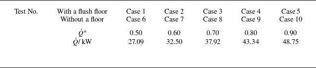
) of 0.50, 0.60, 0.70, 0.80 and 0.90, respectively (table 2). Each experiment lasted 90 s, with a 60 min interval between two. The doors, windows and exhaust system were closed during the experiments to ensure a uniform and quiescent environment.
Experimental conditions.

The SPIV is an optical measurement technique used to measure the three-dimensional instantaneous velocity field of the flow field. The SPIV measurement system involved a dual pulse laser (Nd: YAG laser 200 mJ pulse–1 at 532 nm, 15 Hz, 7 ns pulse–1), two dual frame CCD cameras (FlowSense EO 4M-41 with Nikon 35 mm f/1.8 lens, 2352 × 1768 pixels resolution, 12-bit depth), a time synchroniser and a workstation for image acquisition and processing. The vertical laser sheet was approximately 4 mm thick and passed through the burner centre. The view angle between the two CCD cameras was 30°, and the angle bisector was perpendicular to the laser sheet plane. The spatial resolution for SPIV images was 0.26 mm pixel−1. The PIV images were processed using Dantec DynamicStudio 2015a software by an adaptive PIV algorithm to obtain the velocity fields. This algorithm iteratively adjusted the size and shape of each interrogation area (IA) to adapt to local flow gradients and seeding densities. The first iteration used the 128 × 128 pixel window, and the distance between the IA window and its neighbour was 64 pixels. To maximise the probability of the correlation peak detection, the final interrogation window size of 32 × 32 pixels was chosen to obtain a mean displacement of the particles (for a frame pair) lower than one quarter of the IA size. The flows inside and outside the flame were seeded with solid particles of TiO2 with diameters of 2–3 μm. At the edge of the table, the tracer particles were sprayed upwards along the laser sheet at an angle of 20° to the table by a nitrogen flow with an initial velocity of approximately 5 cm s–1. The calculated Stokes number of St
 $=$
(2.88 ∼ 5.04) × 10–6 was much lower than 0.01, indicating that the tracer particle was small enough to attain the local flow velocity rapidly and exhibited good following characteristics (Liu et al. Reference Liu, Zhang, Wu, Zhang and Lu2017). By analysing the displacement of these particles between image pairs, SPIV can reconstruct the velocity vector in three dimensions for a two-dimensional plane within the flow.
The flames of this work were designed to be buoyancy controlled and turbulent flames based on the literature and dimensionless parameters (Delichatsios Reference Delichatsios1993). Heskestad (Reference Heskestad1988, Reference Heskestad1998) indicated that the free buoyant flame was substantially turbulent for a minimum fire source size d ≥ 0.30 m with
 $\dot{Q}$
> 10 kW. Weckman & Strong (Reference Weckman and Strong1996) found that viscous diffusion is only important near the pool surface (z < 10 cm), and most of the flame is in the turbulent state (
 $\dot{Q}=$
24.60 kW, d
 $=$
30.5 cm). The Rayleigh number
 ${Ra}=(1.16\,{\sim}\,5.61)\times 10^{10}$
was greater than the critical value of 109 for the transition from laminar to turbulent in natural convection. The Froude number
 $\textit{Fr}_{\!f}=(1.42\,{\sim}\,2.56)\times 10^{-4}$
was much less than 0.1, indicating that the flame is buoyancy controlled. Then the flames of this work were turbulent buoyant diffusion flames.
2.2. Flame shape measurement and image process
A Digital Video (DV) camera recorded the flame at 25 f.p.s. with a spatial resolution of 0.71 mm pixel–1. The mean flame height and width were determined by processing the video images. The RGB images (see figure 3
a) were firstly converted into grey scale images (see figure 3
b) and then to binary images (see figure 3
c). The mean value at each pixel of 2400 binary images represented the flame intermittency in each test (see figure 3
d) (Yuan et al. Reference Yuan, Lei and Liu2024). The mean flame height (H) was defined as the axial location with an intermittency of 0.50 at the centreline. The mean flame width (
 $d_{f}$
) was defined as the mean width of the flame probability contours with an intermittency of 0.50.
Calculation of the flame probability contours for
 $\dot{Q}^{*}=$
0.80 in the configuration without a flush floor. (a) Original colour image; (b) grey scale image; (c) binary image; (d) flame probability contours.

2.3. Error analysis
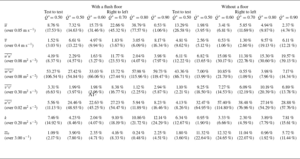
The time-averaged velocities and turbulence statistics should be symmetrical for the free buoyant turbulent diffusion flames. Then the asymmetry of the time-averaged velocities and turbulence statistics could be attributed to the uncertainty of the data. As shown in table 3, two integrated statistical results for the data uncertainty of time-averaged velocities and turbulence statistics are relatively low for different heat release rates (Tieszen et al. Reference Tieszen, O.’Hern, Weckman and Schefer2004; Yuan et al. Reference Yuan, Lei and Liu2024). However, the data uncertainty of the time-averaged radial velocity (
 $\overline{u}$
) is slightly greater when the floor is present compared with that when the floor is absent, which may be attributed to the differences in the distributions of tracer particles around the flame. Since the second-order statistic, i.e. the time-averaged axial and radial fluctuation product (
 $\overline{u'v'}$
) is very small, the uncertainty of
 $\overline{u'v'}$
is significant. In some tests of this work and the experiments of Tieszen et al. (Reference Tieszen, O.’Hern, Weckman and Schefer2004), the uncertainty of
 $\overline{u'v'}$
even exceeded 100 %. Although the number of tracer particles meets the measurement requirements in both the left and right halves, the difference in the number and uniformity of tracer particles in the left and right halves is inevitable. This leads to significant data uncertainty of the right to- left in some cases. By examining the original image, we found that the number and uniformity of tracer particles on the left half were relatively better. Therefore, we present the results of the left half in the subsequent discussion.
Summary of data uncertainty.

 $| \overline{{\textit{Area}}_{\_ 1}}-\overline{{\textit{Area}}_{\_ 2}}| /{\textit{mean}}(\overline{{\textit{Area}}_{\_ 1}},\overline{{\textit{Area}}_{\_ 2}})$
over image area for contours above stated value and in parentheses.
 $| | \overline{{\textit{Area}}_{\_ 1}}-\overline{{\textit{Area}}_{\_ 2}}| +2\sigma | /{\textit{mean}}(\overline{{\textit{Area}}_{\_ 1}},\overline{{\textit{Area}}_{\_ 2}})$
over the image area for contours above stated value.
3. Results and discussion
3.1. Instantaneous flame image and velocity field
Figure 4 is the instantaneous flow field at the vertical plane passing through the burner centreline overlaid on synchronised colour flame images of colour CMOS for
 $\dot{Q}^{*}=$
0.50. In figure 4(a–f), the burner rim was level with the floor, while the floor was absent in figure 4(A–F). Since the gas density in the flame is much lower than the ambient air density, the flame near the burner rim rolls up to form toroidal vortices (see figure 4
a–c and figure 4
A–C) due to the Rayleigh–Taylor instability, which entrains a large amount of ambient air into the flame. Under the action of strong buoyancy, the toroidal vortices accelerate downstream with increasing scale (see figure 4
c–f and figure 4
C–F), and the flame below the toroidal vortices contracts towards the centre axis. Then the toroidal vortices gradually burn out, and a new cycle starts near the burner surface. Notably, in figure 4(e–f), the toroidal vortices break at the flame tip, and the flame is coherent along the burner centreline. However, in figure 4(E–F), as the scale of the toroidal vortices increases steadily, the toroidal vortices could develop to the central axis of the burner, resulting in significant flame shedding. The shedding flame continues to rise and quickly burns out. This could result in stronger axial flame pulsation in the configuration without a floor.
Instantaneous flow fields at the vertical plane passing through the burner centreline overlaid on synchronised colour flame images of colour CMOS for
 $\dot{Q}^{*}=$
0.50. The time interval between adjacent images is 1/15 s. (a)–( f) With a flush floor; (A)–(F) without a floor.

The difference in the development process of the toroidal vortices can be revealed by the following vorticity equation:
 \begin{equation} {\rm D}\boldsymbol{\omega}/{\rm D}t=\big(\boldsymbol{\omega}\boldsymbol{\cdot }\boldsymbol{\nabla }\big)\boldsymbol{V}-\boldsymbol{\omega}\big(\boldsymbol{\nabla }\boldsymbol{\cdot }\boldsymbol{V}\big)+\frac{1}{\rho ^{2}}\left(\boldsymbol{\nabla }\rho \times \boldsymbol{\nabla }p\right)+\frac{\rho _{\infty }}{\rho ^{2}}\big(\boldsymbol{\nabla }\rho \times \boldsymbol{g}\big)+\nu {\nabla} ^{2}\boldsymbol{\omega} ,\end{equation}
where
 $\rho$
, p and g are respectively the gas density, pressure and the gravitational acceleration. The right-hand side terms of (3.1) are the vortex stretching term, dilation term, baroclinic torque, gravitational term and viscous term, respectively. Based on the direct numerical simulation works by Jiang & Luo (Reference Jiang and Luo2000, Reference Jiang and Luo2001), the gravitational term is critical for the creation of flow vorticity in global and local senses and essential to the formation of the large vortical structures in turbulent buoyant diffusion flames.
Figure 5 shows the time-averaged velocity vectors in the central vertical plane and the schematic diagram of
 $(\boldsymbol{\nabla }\rho \times \boldsymbol{g})=| \boldsymbol{\nabla }\rho | | \boldsymbol{g}| \sin (\delta )$
for
 $\dot{Q}^{*}=$
0.50. Here,
 $\delta$
is the angle between
 $\boldsymbol{\nabla }\rho$
and
 $\boldsymbol{g}$
. As shown in figures 5(a) and 5(b), due to the presence of the flush floor, the radial inflow of air at the bottom pushes the flame sheet to be nearly parallel to the burner exit. In figures 5(A) and 5(B), the ambient air flows radially upwards near the burner rim, and the angle (
 $\delta _{wo}$
) between the flame sheet at the burner rim and the burner exit decreases. Then we have
 $\sin (\delta _{w})\lt \sin (\delta _{wo})$
. The subscripts ‘
 $w$
’ and ‘
 $wo$
’ denote with and without the floor, respectively. Consequently, the gravitational term is lower when the floor is present, resulting in a slower increase in tangential vorticity of the toroidal vortices at the bottom of the flame. Compared with the configuration with a flush floor, the scale and vorticity of the toroidal vortices increase faster, and the turbulent mixing rate of fuel and air is greater at the same height for the configuration without a floor (see figure 4
a–f) (Moreno-Boza et al. Reference Moreno-Boza, Coenen, Carpio, Sánchez and Williams2018).
Time-averaged velocity vectors in the central vertical plane for
 $\dot{Q}^{*}=$
0.50 (a, A) and schematic diagram of
 $\boldsymbol{\nabla }\rho \times \boldsymbol{g}$
(b, B): (a) and (b) with a flush floor; (A) and (B) without a floor.

3.2. Mean flame shape
Figures 6(a) and 6(b) show the mean flame shapes of the turbulent buoyant flames with and without the floor for
 $\dot{Q}^{*}=$
0.50–0.90, respectively. All the flames are anchored at the burner rim and exhibit the necking-in effect near the burner exit. With the increase of z, the flame width increases slowly and begins to decrease gradually above a certain height. As
 $\dot{Q}^{*}$
increases, the mean flame shape expands outward steadily. However, the mean flame shapes under the two boundary conditions differ greatly under equal
 $\dot{Q}^{*}$
. Compared with the configuration with a flush floor, the air entrainment rate and the turbulent mixing rate of fuel gas and air both increase in the configuration without a floor, leading to a decrease in the flame height and an increase in the maximum flame width.
Mean flame shapes with an intermittency of 0.50 for the free buoyant diffusion flames. (a) With a flush floor, (b) without a floor.

3.3. Time-averaged velocity field
Figure 7 shows the time-averaged radial velocity (
 $\overline{u}$
) contours in the central vertical plane for
 $\dot{Q}^{*}=$
0.50–0.90 under the two burner boundary conditions. Note that the 0 m s−1 contour is roughly located near the central axis of the burner, which indicates that the flow field exhibits good symmetry. Similar to the experimental results of Weckman & Strong (Reference Weckman and Strong1996) and Tieszen et al. (Reference Tieszen, O’.Hern, Schefer, Weckman and Blanchat2002, Reference Tieszen, O.’Hern, Weckman and Schefer2004), a relatively strong air inflow is formed at the bottom of the flame (z/d
 $\leq$
0.33) due to the presence of the floor. Notably, the contours of
 $0.15\lt \overline{u}\lt 0.30$
m s−1 are tilted upward due to the strong buoyancy of the hot gas in the reactive zone. In the upper part of the flame, the ambient air is mainly engulfed into the flame by the toroidal vortices, named as radial air entrainment. As z increases,
 $\overline{u}$
decreases rapidly. With the increase of
 $\dot{Q}^{*}$
, the profile of
 $\overline{u}$
changes insignificantly. The comparison among figure 7(a–e) and figure 7(A–E) shows that the dimensionless radial locations (
 $\xi =r/b$
) with relatively greater
 $\overline{u}$
(the 0.25 ms−1 contour) are 0.33
 $\leq \xi \leq$
0.67 and 0.67
 $\leq \xi \leq$
1.00 for the configurations with and without a flush floor, respectively. This is consistent with the experimental results of Tieszen et al. (Reference Tieszen, O’.Hern, Schefer, Weckman and Blanchat2002, Reference Tieszen, O.’Hern, Weckman and Schefer2004) (0.30
 $\leq \xi \leq$
0.70, with a flush floor,
 $\dot{Q}^{*}=$
1.73–2.98) and Weckman & Strong (Reference Weckman and Strong1996) (0.67
 $\leq \xi \leq$
1.00, without a floor,
 $\dot{Q}^{*}=$
0.39). Compared with the configuration with a flush floor, the peak value of
 $\overline{u}$
moves towards the burner rim in the configuration without a floor.
Time-averaged radial velocity (
 $\overline{u}$
). (a)–(e) With a flush floor, (A)–(E) without a floor. From left to right in each row,
 $\dot{Q}^{*}=$
0.50, 0.60, 0.70, 0.80 and 0.90, respectively; r
 $=$
0 cm denotes the burner centreline.

Figure 8 presents the time-averaged axial velocity (
 $\overline{v}$
) in the central vertical plane under different
 $\dot{Q}^{*}$
and burner boundary conditions. Near the surface of the burner,
 $\overline{v}$
is only a few cm s–1. The centreline
 $\overline{v}$
increases rapidly to around 2.60 m s−1 due to the strong buoyancy of hot gas in the flame. As z increases, the flow changes from the laminar state to the turbulent state, and the radial profile of
 $\overline{v}$
gradually changes from a ‘top-hat’ profile to a Gaussian profile. Similar to the experimental results of Tieszen et al. (Reference Tieszen, O.’Hern, Weckman and Schefer2004), as
 $\dot{Q}^{*}$
increases, the radial profile of
 $\overline{v}$
varies from a unimodal to a bimodal type due to the increase of the fuel-rich core size. As shown in the discussion of figure 5, compared with the configuration with a flush floor (see figure 8
a–e), the mixing rate of fuel gas and air increases (see figure 8
A–E), and the fuel-rich core scale would be smaller in the configuration without a floor under equal
 $\dot{Q}^{*}$
. The transition of the radial profile of
 $\overline{v}$
from unimodal to bimodal is more pronounced in the configuration with a flush floor.
Time-averaged axial velocity (
 $\overline{v}$
). (a)–(e) With a flush floor, (A)–(E) without a floor. From left to right in each row,
 $\dot{Q}^{*}=$
0.50, 0.60, 0.70, 0.80 and 0.90, respectively; r
 $=$
0 cm denotes the burner centreline.

3.4. Time-averaged turbulent statistics
Figure 9 presents the contour maps of the time-averaged radial velocity fluctuations squared (
 $\overline{u'u'}$
) in the central vertical plane under different
 $\dot{Q}^{*}$
and burner boundary conditions. It is found that
 $\overline{u'u'}$
is relatively small near the burner surface (z/d < 0.33), but increases rapidly with the increase of z. In the radial direction,
 $\overline{u'u'}$
first increases and then decreases, and its radial profile is bimodal. As
 $\dot{Q}^{*}$
increases, the contour area of
 $\overline{u'u'}=$
0.18 m2 s−2 increases slightly, indicating that the radial flame pulsations are enhanced gradually. In figure 9(a–e) and the experiments of Tieszen et al. (Reference Tieszen, O’.Hern, Schefer, Weckman and Blanchat2002, Reference Tieszen, O.’Hern, Weckman and Schefer2004) (
 $\dot{Q}^{*}=$
1.73–2.98, with a flush floor), the maximum
 $\overline{u'u'}$
values in the radial direction are located at approximately
 $\xi =0\mathit{.}47$
and
 $\xi =0\mathit{.}40$
, respectively. However, the maximum value of
 $\overline{u'u'}$
is found near
 $\xi =0\mathit{.}67$
in figure 9(A–E) (without a floor). Consistent with figure 5, the gravitational term at the flame bottom is larger when the floor is absent, and the toroidal vortices grow quickly. This also results in the differences among figure 9(a–e) and figure 9(A–E). Compared with the configuration with a flush floor, the area of the
 $\overline{u'u'}=$
0.18 m2 s−2 contour is much greater in the configuration without a floor under the same
 $\dot{Q}^{*}$
, indicating that the radial pulsation of turbulent buoyant flames is stronger in the configuration without a floor.
Time-averaged radial velocity fluctuations squared (
 $\overline{u'u'}$
). (a)–(e) With a flush floor, (A)–(E) without a floor. From left to right in each row,
 $\dot{Q}^{*}=$
0.50, 0.60, 0.70, 0.80 and 0.90, respectively; r
 $=$
0 cm denotes the burner centreline.

Figure 10 presents the time-averaged axial velocity fluctuations squared (
 $\overline{v'v'}$
) in the central vertical plane under different
 $\dot{Q}^{*}$
and burner boundary conditions. Similar to the time-averaged axial velocity (
 $\overline{v}$
), the maximum
 $\overline{v'v'}$
occurs around the central axis and
 $\overline{v'v'}$
increases rapidly when z increases. With the increase of
 $\dot{Q}^{*}$
, the radial profile of
 $\overline{v'v'}$
near the burner surface changes from unimodal to bimodal. Compared with the configuration with a flush floor, the axial location where the flame shedding occurs is lower in the configuration without a floor (see figure 4). Consequently, at the same height,
 $\overline{v'v'}$
in the configuration without a floor (see figure 10(A)–10(E)) is greater than that in the configuration with a flush floor (see figure 10
a–e). The comparison among figure 10(a–e) and figure 10(A–E) indicates that
 $\overline{v'v'}$
is relatively lower in the configuration with a flush floor, i.e. the presence of the floor suppresses the axial flame pulsation. As shown in figures 9 and 10,
 $\overline{v'v'}$
is approximately 0.10 m2 s−2 −1.00 m2 s−2, and
 $\overline{u'u'}$
ranges from 0.02 m2 s−2 to 0.18 m2 s−2. Therefore, the axial pulsation is more significant than the radial pulsation, and the turbulent flow is anisotropic in turbulent buoyant diffusion flames (Kundu, Cohen & Dowling Reference Kundu, Cohen and Dowling2016).
Time-averaged axial velocity fluctuations squared (
 $\overline{v'v'}$
). (a)–(e) With a flush floor, (A)–(E) without a floor. From left to right in each row,
 $\dot{Q}^{*}=$
0.50, 0.60, 0.70, 0.80 and 0.90, respectively; r
 $=$
0 cm denotes the burner centreline.

Figure 11 shows the time-averaged axial and radial fluctuation product (
 $\overline{u'v'}$
) in the central vertical plane of flames with and without a floor for 0.50
 $\leq \dot{Q}^{*} \leq$
0.90. Near the burner surface,
 $\overline{u'v'}$
is relatively small. As z increases,
 $\overline{u'v'}$
gradually increases. When z reaches a certain height,
 $\overline{u'v'}$
remains unchanged with the increase of z. In the radial direction,
 $\overline{u'v'}$
first increases and then decreases, and its radial profile is the bimodal type. With the increase in
 $\dot{Q}^{*}$
, the lowest height (z) of the contour
 $| \overline{u'v'}|=$
0.06 m2 s−2 increases. The peaks of
 $\overline{u'v'}$
are located in the normalised radial locations of
 $\xi \approx 0\mathit{.}33$
and
 $\xi \approx 0\mathit{.}67$
in the configurations with and without a floor, respectively. Compared with the configuration with a flush floor, the radial location of the peak
 $\overline{u'v'}$
moves closer to the burner rim in the configuration without a floor.
Time-averaged axial and radial fluctuation product (
 $\overline{u'v'}$
). (a)–(e) With a flush floor, (A)–(E) without a floor. From left to right in each row,
 $\dot{Q}^{*}=$
0.50, 0.60, 0.70, 0.80 and 0.90, respectively; r
 $=$
0 cm denotes the burner centreline.

Similar to the experimental results of Yuan et al. (Reference Yuan, Lei and Liu2024) for the configuration without a floor with
 $0.2\lt \dot{Q}^{*}\lt 0.5$
, the peak of time-averaged tangential velocity fluctuations squared (
 $\overline{w'w'}$
) is located on the central axis of the burner. In the configuration with a flush floor,
 $\overline{w'w'}$
is 0.05–0.30 m2 s−2. In the configuration without a floor, it becomes 0.05–0.40 m2 s−2. Figure 12 shows the turbulent kinetic energy (
 $k=(\overline{u'u'}+\overline{v'v'}+\overline{w'w'})/2$
) in the central vertical plane. The spatial distributions of
 $k$
and
 $\overline{v'v'}$
are similar, and their magnitudes are close (10−1 m2 s−2). The maximum
 $k$
and
 $\overline{v'v'}$
are both located on the burner centreline. As the height (z) increases,
 $k$
gradually increases. Since
 $\overline{v'v'}$
is approximately one order of magnitude greater than
 $\overline{u'u'} , k$
is determined by
 $\overline{v'v'}$
in the free turbulent buoyant diffusion flame. As
 $\dot{Q}^{*}$
increases, the radial profile of k near the burner surface changes from the unimodal to the bimodal type. Compared with the configuration with a flush floor (see figure 12
a–e), the flame pulsation is stronger and k increases slightly in the configuration without a floor under equal
 $\dot{Q}^{*}$
.
Turbulent kinetic energy (k). (a)–(e) With a flush floor, (A)–(E) without a floor. From left to right in each row,
 $\dot{Q}^{*}=$
0.50, 0.60, 0.70, 0.80 and 0.90, respectively; r
 $=$
0 cm denotes the burner centreline.

Figure 13 shows the time-averaged tangential vorticity (
 $\overline{\omega }_{\theta }$
) in the vertical plane passing through the burner centreline. As shown by figure 13(a–e) and figure 13(A–E), although the peak value of
 $\overline{\omega }_{\theta }$
varies slightly in the two configurations with and without a floor, the area with
 $| \overline{\omega }_{\theta }| \gt$
3.00 s−1 in the configuration without a floor is much larger than that in the configuration with a flush floor under equal
 $\dot{Q}^{*}$
. This indicates that the growth of toroidal vortices is faster when the floor is absent, which is consistent with the discussion in § 3.1. As
 $\dot{Q}^{*}$
increases, the initial fuel velocity at the burner exit increases, and the lowest height of
 $\overline{\omega }_{\theta }=$
12.00 s−1 gradually increases.
Time-averaged tangential vorticity (
 $\overline{\omega }_{\theta }$
). (a)–(e) With a flush floor, (A)–(E) without a floor. From left to right in each row,
 $\dot{Q}^{*}=$
0.50, 0.60, 0.70, 0.80 and 0.90, respectively; r
 $=$
0 cm denotes the burner centreline.

3.5. The mean turbulent viscosity
The turbulent viscosity (
 $\nu _{t}$
) is a local function in the flow (Katopodes Reference Katopodes2019). Based on the gradient transport approximation,
 $\nu _{t}$
could be determined by
 $\nu _{t}=-\overline{u'v'}/(\partial \overline{v}/\partial r)$
. For turbulent buoyant flames,
 $\overline{u'v'}$
and
 $\overline{v}$
are assumed to have self-similarity and can be written as
 \begin{align} &\overline{v}=\overline{v}_{m}\exp \big(-C_{1}\xi ^{2}\big),\end{align}
 \begin{align} \overline{u'v'}&=\textit{fcn}\left(\dot{Q},d,\rho _{\infty },c_{p},g,T_{\infty }\right)\phi \left(\xi \right)\!.\end{align}
Here, the radial profile of
 $\overline{u'v'}$
(
 $\phi$
) is taken as
 $\phi (\xi )=\xi (C_{2}+C_{3}\xi ^{3})(1+C_{4}\xi ^{3})^{-6}$
, which is suggested by Shabbir & George (Reference Shabbir and George2006) for a round buoyant plume and satisfies the boundary conditions of
 $\phi (0)=\phi (\infty )=0$
. Also, C
1, C
2, C
3 and C
4 are dimensionless parameters. Since the fire buoyancy flux
 $F=g\dot{Q}/(\rho _{\infty }c_{p}T_{\infty })$
, (3.3) can be written as
 $\overline{u'v'}=fcn(F,d,\overline{v}_{m})\phi (\xi )$
. Based on the dimensional analysis, we obtain
 \begin{equation} \overline{u'v'}=\overline{v}_{m}F^{1\mathit{/}3}d^{-1\mathit{/}3}\phi \left(\xi \right)\!.\end{equation}
Figure 14 shows the radial profile of
 $\overline{v}$
and
 $\overline{u'v'}$
under the two burner configurations. Near the surface of the burner, the initial laminar flow becomes turbulent quickly. To reduce the impact of the bottom transition zone, the data above the height where
 $| \overline{u'v'}|=$
0.02 are used for analysis. All data sets of
 $\overline{v}$
and
 $\overline{u'v'}$
could be correlated well by (3.2) and (3.4), respectively. The radial profiles of
 $\overline{v}$
and
 $\overline{u'v'}$
are unimodal and bimodal, respectively. As shown in figures 14(a) and 14(A), the time-averaged axial velocity (
 $\overline{v}$
) decreases quicker in the radial direction in the configuration with a flush floor. In figures 14(b) and 14(B), the maximum
 $\overline{u'v'}$
values are located around
 $\xi =0\mathit{.}40$
and
 $\xi =0\mathit{.}58$
for the configurations with and without a floor, respectively.
Radial profiles of
 $\overline{v}$
and
 $\overline{u'v'}$
: (a) and (b) with a flush floor; (A) and (B) without a floor.

Substituting (3.2) and (3.4) into
 $\nu _{t}=-\overline{u'v'}/(\partial \overline{v}/\partial r)$
, the local turbulent viscosity (
 $\nu _{t}$
) is given by
 \begin{equation} \nu _{t}=F^{1/3}d^{2/3}{\Phi} \left(\xi \right)\!,\end{equation}
where
 ${\Phi} (\xi )=(4C_{1}\xi )^{-1}\phi (\xi )\exp (C_{1}\xi ^{2})$
. Assuming that (3.5) is applicable within the mean flame height (z
 $\leq$
H), then the mean
 $\nu _{t}$
within the flame height is written as
 \begin{equation} \nu _{t}^{=}=\lambda F^{1/3}d^{2/3} ,\end{equation}
where the turbulent viscosity coefficient
 $\lambda =\xi _{1}^{-1}\int _{0}^{\xi _{1}}{\Phi} (\xi )\,\rm d\xi$
. The integration upper limit
 $\xi _{1}$
is taken as the maximum radial range of measurement at
 $\xi _{1}=$
0.98. Note that previous works have shown that
 $\nu _{t}^{=}=\lambda _{1}F^{1/2}H^{3/2}$
for
 $\dot{Q}^{*}\gt 1$
(Lei & Liu Reference Lei and Liu2017) and
 $\nu _{t}^{=}=\lambda _{2}g^{1/2}d^{3/2}$
for
 $0.2\lt \dot{Q}^{*}\lt 0.5$
(Yuan et al. Reference Yuan, Lei and Liu2024). In this work,
 $\nu _{t}^{=}$
is scaled by the fire buoyancy flux (F) and fire source diameter (d) for
 $0.5\leq \dot{Q}^{*}\lt 1$
, regardless of the flame height (H).
Table 4 presents the data processing results under different
 $\dot{Q}^{*}$
and burner boundary conditions. The turbulent viscosity coefficients are
 $\lambda _{w}=(0\mathit{.}77\pm 0\mathit{.}06)\times 10^{-2}$
and
 $\lambda _{wo}=(1\mathit{.}03\pm 0\mathit{.}16)\times 10^{-2}$
for the configurations with and without a floor, respectively. Substituting
 $\lambda _{w}$
and
 $\lambda _{wo}$
into (3.6), the mean turbulent viscosities are respectively
 $\nu^{=} _{t\,w}=$
0.0032∼0.0038 m2 s−1 and
 $\nu^{=} _{t\,w}=$
0.0042∼0.0051 m2 s−1 for the configurations with and without a floor under different
 $\dot{Q}^{*}$
. Note that the mean turbulent viscosity is one order of magnitude larger than the air viscosity (
 $\nu=$
1.63 × 10⁻⁴ m2 s−1) in the flame (1200 K). Moreover, under equal
 $\dot{Q}^{*} , \nu^{=} _{t\,w}$
is significantly greater than
 $\nu^{=} _{t\,w}$
. Therefore, it is inferred that the presence of the floor around the burner could reduce the turbulent mixing rate of fuel and air in turbulent buoyant flames.
Data processing results.

3.6. Flame shape formulations based on turbulent transport properties
3.6.1. Flame height correlation
For the lightly sooting flames, the theoretical flame height should be close to the visible flame height determined by the DV images. The theoretical flame height (H) could be defined as the distance between the burner exit and the axial position where the mixture fraction
 $Z=Z_{st}$
at the flame central axis. The mixture fraction
 $Z$
is defined by
 $Z=(sY_{F}-Y_{O}+Y_{O,\infty })/(s+Y_{O,\infty }) , Y_{F}$
and
 $Y_{O}$
are the mass fractions of fuel and oxygen,
 $s=(a_{O}M_{O})/(a_{F}M_{F})$
is the mass stoichiometric ratio of oxygen to fuel,
 $a_{O}$
are
 $a_{F}$
the coefficients of fuel and oxygen in an overall unique reaction and
 $M_{O}$
and
 $M_{F}$
are respectively the molecular weights of fuel and oxygen. Here,
 $Z_{st}=Y_{O,\infty }/(s+Y_{O,\infty })$
is the stoichiometric value. Lei & Liu (Reference Lei and Liu2017) derived the flame height correlation by solving the controlling equation of mixture fraction through coordinate transformation
 \begin{equation} \frac{H}{d}=\frac{v_{F0}d}{4\left(D^{=}+D_{t}^{=}\right)}\frac{1}{4\ln \left[1/\left(1-Z_{st}\right)\right]} .\end{equation}
In the derivation of (3.7), the boundary conditions at the bottom apply to the turbulent diffusion flames for the configurations with and without a floor. Therefore, (3.7) should be able to provide accurate estimations of the flame heights under the two burner boundary conditions in this work. In the fully turbulent flow, the mean molecular diffusivity (
 $D^{=}$
) can be ignored compared with the mean turbulent diffusivity within the mean flame height (
 $D_{t}^{=}$
).
 $D_{t}^{=}$
could be related to the mean turbulent viscosity (
 $v_{t}^{=}$
) through the turbulent Schmidt number (
 $Sc_{t}=v_{t}^{=}/D_{t}^{=}$
)
 \begin{equation} D_{t}^{=}=\lambda {Sc}^{=-1}_{t}F^{1/3}d^{2/3} .\end{equation}
Substituting (3.8) into (3.7) yields
 \begin{equation} H^{*}=\left\{\frac{Sc_{t}^{=}}{4\pi \lambda }\frac{\rho _{\infty }c_{p}T_{\infty }}{{\unicode[Arial]{x0394}} H_{c}\rho _{0}}\frac{1}{\ln \left[1/\left(1-Z_{st}\right)\right]}\right\}\dot{Q}^{*2/3}=\kappa \dot{Q}^{*2/3} ,\end{equation}
or
 \begin{equation} H=\kappa \dot{Q}^{*2/3}d=\kappa L_{0}^{5/3}d^{-2/3} ,\end{equation}
where
 $L_{0}=[\dot{Q}/(\rho _{\infty }c_{p}T_{\infty }g^{1/2})]^{2/5}$
. Equation (3.9) reproduced the classical ‘2/3’ exponential dependence of
 $H^{*}$
on
 $\dot{Q}^{*}$
for 0.5
 $\leq \dot{Q}^{*}$
< 1 in Drysdale (Reference Drysdale2011). However, the coefficient
 $\kappa$
is a deterministic function of the turbulent transport characteristics, fuel and ambient parameters in (3.10). For the two configurations with and without a flush floor under equal
 $\dot{Q}^{*} , \kappa$
is only affected by the turbulent viscosity coefficient (
 $\lambda$
), and we have
 $H_{w}/H_{wo}=\lambda _{\textit{ratio}}^{-1}=(\lambda _{w}/\lambda _{wo})^{-1}$
.
3.6.2. Flame width correlation
For vertical turbulent diffusion flames, the axial convection time of fuel from the burner exit to the flame tip
 $(t_{conv}=\int _{0}^{H}\overline{v}_{c}^{-1}{d}z)$
is approximately equal to the radial diffusion time of air from the flame edge to the flame centreline
 $(t_{\textit{diff}}=d_{f}^{2}/(8D_{t}))$
(Jost Reference Jost1946; Saito, Williams & Gordon Reference Saito, Williams and Gordon1986; Sunderland et al. Reference Sunderland, Mendelson, Yuan and Urban1999; Lei et al. Reference Lei, Huang, Liu and Zhang2022b
). Then we have
 \begin{equation} d_{f}^{2}=8D_{t}\int _{0}^{H}\overline{v}_{c}^{-1}{d}z=16D_{t}k^{-1}H^{1/2} ,\end{equation}
where
 $\overline{v}_{c}=k_{0}z^{1/2}$
(McCaffrey Reference McCaffrey1979). The subscript ‘c’ denotes the centreline. It is found that
 $k_{0}$
varies slightly under different
 $\dot{Q}^{*}$
and burner boundary conditions in this work. For simplicity,
 $k_{0}$
is taken as 5.00 m2 s−1. Using (3.8) and (3.9) in (3.11) leads to
 \begin{equation} d_{f}=KL=K\dot{Q}^{*1/3}d=KL_{0}^{5/6}d^{1/6} .\end{equation}
The characteristic length L and the dimensionless constant K are respectively
 \begin{align}& L=\left(\frac{\dot{Q}d^{1/2}}{\rho _{\infty }c_{p}T_{\infty }g^{1/2}}\right)^{1/3}=\dot{Q}^{*1/3}d=L_{0}^{5/6}d^{1/6} , \\[-28pt] \nonumber \end{align}
 \begin{align}&\quad K=4Sc_{t}^{=-1/2}g^{1/4}\kappa ^{1/4}k_{0}^{-1/2}\lambda ^{1/2} .\end{align}
Note that
 $L_{0}$
is the sole characteristic length in the correlations of
 $H$
and
 $d_{f}$
for
 $\dot{Q}^{*}$
> 1 (Quintiere Reference Quintiere2006; Lei et al. Reference Lei, Huang, Liu and Zhang2022b
). However, for 0.5
 $\leq \dot{Q}^{*}$
< 1, the characteristic length scales are
 $L_{0}^{5/3}d^{-2/3}$
and
 $L_{0}^{5/6}d^{1/6}$
in (3.10) and (3.12), respectively. Then, the dimension of the fire source (d) becomes an important length scale affecting the combustion behaviour of free buoyant flames (Zukoski, Kubota & Cetegen Reference Zukoski, Kubota and Cetegen1981; Zukoski, Cetegen & Kubota Reference Zukoski, Cetegen and Kubota1985). In addition, (3.13) indicates that
 $d_{f}$
is proportional to d for turbulent buoyant flames under equal
 $\dot{Q}^{*}$
. For the two configurations with and without a flush floor, it could be concluded that
 $d_{fw}/d_{fwo}=\lambda _{\textit{ratio}}^{1/4}$
from (3.14).
3.6.3. Verification of the flame height and width correlations
By substituting
 $\lambda _{w}=0\mathit{.}77\times 10^{-2}$
and
 $\lambda _{wo}=1\mathit{.}03\times 10^{-2}$
into (3.9) and (3.14), we have
 $\kappa _{w}=$
3.99,
 $\kappa _{wo}=$
2.99,
 $K_{w}=$
0.45 and
 $K_{wo}=$
0.49 for the methane buoyant flames with and without a floor in this work, respectively. In the calculation of
 $\kappa$
and
 $K , Z_{st}=0.055 , Sc_{t}^{=}=0.75 , {\unicode[Arial]{x0394}} H_{c}=$
50 × 103 kJ kg−1,
 $\rho _{\infty }=$
1.1614 kg m−3,
 $c_{p}=$
1.007 kJ kg−1 K−1,
 $T_{\infty }=$
300 K and
 $\rho _{0}=$
0.2403 kg m−3 is the geometric mean of the methane density at the burner exit of 600 K and air density at the average flame temperature of 1500 K (Chuah et al. Reference Chuah, Kuwana, Saito and Williams2011). In addition, the coefficients
 $\kappa _{w}=$
3.99 and
 $\kappa _{wo}=$
2.99 are comparable to the fitted values of
 $\kappa=$
2.6 and 3.30 by Zukoski et al. (Reference Zukoski, Cetegen and Kubota1985) and Delichatsios (Reference Delichatsios1987), respectively.
In the derivation of (3.10) and (3.12), there are some deviations between the assumptions and the actual situation. (i) The influence of the axial diffusion term on flame height was neglected in the derivation of (3.7). This may result in a relatively lower prediction of the mean flame height (Lee & Chung Reference Lee and Chung1991; Mahalingam Reference Mahalingam1993; Ban, Venkatesh & Saito Reference Ban, Venkatesh and Saito1994; Knott & Brewster Reference Knott and Brewster2000). (ii) The model ignored the transition of flames near the burner surface from laminar flame to turbulent flame. (iii) Although the methane flames of this work involve relatively less visible soot, the differences between the theoretical and visual flame heights and widths are inevitable. To include the potential effects of these factors, we added the correction factors on the right-hand sides in (3.9) and (3.12). Figure 15 presents the comparisons between the experimental and the predicted mean flame heights and widths for free buoyant flames with and without a floor of this work. The predicted results are in good agreement with the experimental data within an error range of ±10 %. The four correction coefficients of 0.93, 0.92, 0.95 and 0.99 are all close to unity, indicating that the models have good predictive ability and the influence of the above three factors is not significant. However, future works are demanded to study the influence of burner boundary conditions under larger burner scales.

4. Conclusions
This paper investigated the effects of the fuel mass flux and the burner boundary condition on the turbulent transport characteristics and flame shape of free turbulent buoyant diffusion flames with
 $\dot{Q}^{*}=$
0.50–0.90. The velocity fields and the mean flame shapes of turbulent buoyant diffusion flames with and without a floor were compared in detail. Key findings of this study include the following.
In turbulent buoyant diffusion flames, the radial profiles of time-averaged axial velocity (
 $\overline{v}$
), the time-averaged axial velocity fluctuations squared (
 $\overline{v'v'}$
) and turbulent kinetic energy (k) are unimodal, while the radial profiles of time-averaged radial velocity (
 $\overline{u}$
), the time-averaged radial velocity fluctuations squared (
 $\overline{u'u'}$
) and the time-averaged axial and radial fluctuation product (
 $\overline{u'v'}$
) are bimodal. As
 $\dot{Q}^{*}$
increases, the scale of the fuel-rich core gradually increases. Due to the relatively low buoyancy in the fuel-rich core, the radial profiles of
 $\overline{v} , \overline{v'v'}$
, and k near the burner exit change from the unimodal type to the bimodal type.
Compared with the configuration without a floor under equal
 $\dot{Q}^{*}$
, the transition of the radial profile of time-averaged axial velocity (
 $\overline{v}$
), the time-averaged axial velocity fluctuations squared (
 $\overline{v'v'}$
) and the turbulent kinetic energy (k) near the burner surface from unimodal to bimodal is more pronounced, and the radial locations of the maximum time-averaged radial velocity (
 $\overline{u}$
), the time-averaged radial velocity fluctuations squared (
 $\overline{u'u'}$
) and the time-averaged axial and radial fluctuation product (
 $\overline{u'v'}$
) move closer to the central axis of the burner in the configuration with a flush floor.
Based on the dimensional analysis and the gradient transport assumption, the correlation of the mean turbulent viscosity for a turbulent buoyant diffusion flame within
 $0.5\leq \dot{Q}^{*}\lt 1$
is found to be
 $\nu _{t}^{=}=\lambda F^{1/3}d^{2/3}$
. The turbulent mixing mechanism of fuel and air changes in different
 $\dot{Q}^{*}$
regimes.
Based on the concept of turbulent transport and the assumptions of equal axial convection and radial diffusion times, semi-physical models of
 $H^{*}=\kappa \dot{Q}^{*2/3}$
and
 $d_{f}=K\dot{Q}^{*1/3}d$
are derived for the mean flame height and width, respectively. The coefficients of
 $\kappa$
and
 $K$
are deterministic functions of turbulent transport characteristics, fuel properties and ambient parameters. The ratio of the mean flame heights and the ratio of the mean flame widths between the configurations with and without a floor depend on the ratio of the mean turbulent viscosity coefficients by the -1 and 1/4 power laws, respectively.
The predicted results agree well with the experiments of free turbulent buoyant flames of
 $0.5\leq \dot{Q}^{*}\leq 0.9$
in this work. The presence of the flush floor leads to the reduction of the mean turbulent mixing rate, leading to an increase in the mean flame height and a decrease in the mean flame width.
Funding
This work was sponsored by the National Natural Science Foundation of China (Nos. 52222605, 52321003). J.L. is supported by the Youth Innovation Promotion Association of CAS (No. 2022462).
Author contributions
Y. Yuan: Writing – original draft, Visualisation, Validation, Methodology, Investigation, Formal analysis, Data curation, Conceptualisation. J. Lei: Writing – review & editing, Supervision, Resources, Project administration, Methodology, Funding acquisition, Data curation, Conceptualisation. N. Liu: Writing – review & editing, Supervision, Resources, Project administration, Funding acquisition, Conceptualisation. W. Gao: Writing – review & editing, Conceptualisation.
Declaration of interest
The authors declare that they have no known competing financial interests or personal relationships that could have appeared to influence the work reported in this paper.