

1 Introduction
During macroeconomic shocks the aggregate measurement of performance is important for policymakers and the general public. After all, the first coordinated estimates of national income in the United States were produced in the 1930s during the single most significant downturn of the 20th or 21st centuries. Further, World War II, and the need for planning of wartime production, motivated annual estimation of national product (USBEA, 2006). Such measurement tends to focus on “conventional” or market-oriented indicators such as unemployment, gross output, as well as indexed measures of prices and consumer confidence. Comprehensive mensuration of performance should also encompass evaluation of public policy. Such assessment of laws, rules, and statutes often assumes the form of benefit-cost analysis (BCA). The importance of BCA intensifies during downturns as public resources are stretched thin and sensitivity to policy-induced distortions is magnified as resilience declines.Footnote 1
For large-scale policies it is common place for analysts to characterize impacts in terms of changes in Gross Domestic Product (GDP) or GDP growth (CBO, 2012). Whether or not policy impacts are captured by conventional macroeconomic aggregates such as GDP depends on the nature of the policy in question. Certain programs may have effects largely within the market boundary. In such contexts, market-oriented indices capture the ramifications of policy. However, for environmental BCA it seems likely (if not probable) that some outcomes manifest outside the market boundary.Footnote 2 Relying on GDP to measure the consequences of environmental policy is problematic because GDP does not, as currently defined, encompass extra-market consequences.
The problem, however, is worse than simply obtaining an incomplete picture of policy outcomes. Reliance on the extant national accounts for environmental policy assessment yields not only a partial assessment of policy but a potentially biased appraisal because the “C” of BCA are in market indicators, while the “B” are not. This argument is especially important during recessions because, during such adverse shocks, the drumbeat in the popular press and among some political circles against environmental policy rises to a fever pitch. Often this argument emphasizes the “jobs-environment” tradeoff. Studies that have explored this issue empirically find mixed results.Footnote 3 Whether employment effects from environmental policy are transient or more long term depends on if the economy is operating efficiently. Claims that regulatory-induced labor market impacts are enduring and harmful have merit especially if the economy is not operating efficiently (Haveman & Weimer, Reference Haveman and Weimer2015). Regardless, the present article is not taking the position that labor market effects are inconsequential: rather that BCA and public discourse needs to encompass both benefits and costs.
So, if not GDP what should the policy community employ to succinctly and accurately convey policy consequences? To answer this, the current paper demonstrates a new connection between BCA and the National Income and Product Accounts (NIPAs). The article computes an augmented measure of GDP, Environmentally Adjusted Value Added (EVA), (Muller, Reference Muller2014a ,Reference Muller, Jorgensen, Landefeld and Schreye b ), which is defined as GDP less environmental pollution damage. Environmental policy BCA is incorporated directly into the EVA in two ways. In a particular time period, damages from pollution emissions are deducted from market GDP in a standard with-and-without policy comparison.Footnote 4 Second, secular changes in damages, output (GDP), and correspondingly, in the EVA are employed to estimate augmented rates of growth. Comparison to a no-policy counterfactual then yields the effect of the policy on the augmented measure of EVA growth.
Admittedly, this approach is justified only for policies and programs that have the potential to yield large enough effects as to be detectable in the NIPAs and the regional accounts. Prior research has demonstrated that the consequences of the Clean Air Act and air pollution, generally, in the United States are large relative to GDP (USEPA, 1999, 2010, 2011a ). Further, the National Academies of Science’s National Research Council (NAS NRC) alluded to the potential importance of an augmented accounting system specifically focusing on air pollution damage during periods of rapid emission reductions (NAS NRC, Reference Nordhaus and Kokkelenberg1999, p. 147). This latter reference is especially relevant to the 2008–2011 time period as macroeconomic conditions and air pollution policy both conspired to reduce emissions. Thus, data and modeling capabilities as well as the magnitude of the Act bolster the focus on air pollution as a test case for the synthesis of BCA and the NIPAs.
Importantly, the present paper is not proposing that EVA is a comprehensive measure of economic welfare. As it is well known that indices such as GDP does not measure welfare, the EVA does not either. Rather, the EVA adjusts GDP to demonstrate (1) the potential importance of using an index that includes both the benefits and costs of environmental policy, and (2) it does so in a context with established methodology that has been extensively used in prior BCA (USEPA, 1999, 2011a ).
To explore the potential synthesis of BCA with the NIPAs, this article asks: how did adoption of abatement technology for sulfur dioxide (SO2) affect an augmented measure of output that deducts environmental cost from GDP?Footnote 5 Since the direct costs of purchasing, installing, and operating abatement technology are already in GDP, the monetary benefits of pollution control are the critical augmentation in this context. The use of abatement devices specifically for SO2 is a costly action undertaken by firms because of regulation. For example, the capital cost for a flue-gas desulfurization (FGD) unit installed on a new 500 MW generator is reported to range from $110 million to $150 million (Sargent and Lundy, 2007). Investments of this magnitude (that do not yield private or internal benefits to the firm) must be induced. In particular, scrubbing technology adoption is due to incentives or mandates established by the Clean Air Act which may manifest directly through federal policy or indirectly through state implementation of the Act. In either case, the adoption of scrubbing technology is due to a policy intervention. Thus, application of some form of BCA is appropriate.
The empirical analysis exploits detailed, facility-level data regarding the use of particular abatement technologies. The United States Environmental Protection Agency (USEPA) and the U.S. Department of Energy (USDOE) report the type and timing of adoption of FGD units, also known as scrubbers, among the power generation fleet in the United States. In addition, both agencies report annual consumption of fuel by plants, net generation of electricity, and emissions of SO2. Capitalizing on these data, the analysis employs reported emissions and an integrated assessment model (IAM) to estimate damages corresponding to observed emissions. The paper then constructs a counterfactual scenario in which the documented adoption of abatement devices did not occur. Rather, emissions rates are assumed to have persisted at their pre-abatement intensities. Counterfactual emissions are estimated as the product of the pre-abatement emissions rates (expressed in tons/million btu (mmbtu) of fuel consumed) times post-abatement generation (expressed in mmbtu). The resulting tonnage is processed through the IAM. In both the observed and counterfactual cases, damages are tabulated in accord with the principles established in the NIPAs and in previous research (Nordhaus, Reference Nordhaus, Jorgensen, Landefeld and Nordhaus2006; Muller, Mendelsohn & Nordhaus, Reference Muller, Mendelsohn and Nordhaus2011; Muller, Reference Muller2014a ,Reference Muller, Jorgensen, Landefeld and Schreye b ); gross external damage (GED) is computed as the product of plant-specific marginal damage and reported or counterfactual emissions for each case. Then, EVA (defined as GDP – GED) is estimated with and without the use of abatement technology. In a particular time period, this facilitates a test of whether the use of abatement technology has a detectable effect on EVA levels. (See Figure 1 for a schematic representation of the BCA design which is an application of the method to the state of West Virginia.)
Schematic Demonstration of BCA: West Virginia.

This simulation design is implemented in three time periods: 2005, 2008, and 2011. The years of 2005, 2008, and 2011 are selected for study because, first, USEPA reports national emission inventories in these three years. Second, the power generation fleet in the United States made a significant investment in scrubbing technology between 2005 and 2011 (USDOE, 2014), (see Figure 2). It is therefore conceivable that the benefits and costs due to adoption of FGD units are large enough to be detected in the EVA.
Use of FGD by Facilities in the Acid Rain Program: 1995–2011.

With emission observations for 2005 and 2011, the simulations identify FGD units adopted between 2005 and 2011. Then, observed and counterfactual emission estimates for 2008 and 2011 are used to estimate observed and counterfactual pollution damage and EVA. EVA growth between 2005 and 2011 is computed with and without newly installed scrubbing technology. The second set of simulations repeats this design for each of the subtime periods: 2005–2008, and 2008–2011. This last comparison is targeted to explore how FGD adoption in the years immediately preceding and then during the Great Recession affected augmented growth rates.
1.1 State and Regional Accounts: Are EVA growth rates illusory?
The BCA exercise conducted in this paper tracks FGD installation at particular power generation facilities. At the most aggregated level, the article reports the effects of FGD use on EVA across all states that installed scrubbing units within the time periods under examination. To connect the adoption of pollution abatement technology to a measure of state economic performance, the U.S. Bureau of Economic Analysis (USBEA) state accounts are employed to compute state EVA. Then, in accord with the simulation design described above, EVA levels and growth are estimated for each state that put FGD units in place.
Computing state GED raises difficult accounting issues; in particular how one interprets differences in EVA and GDP growth, which are related to those initially discussed by Nordhaus (Reference Nordhaus2008). By reporting GED and EVA regionally, the appearance is that the beneficiaries of EVA growth due to GED reduction lie within that region. This is, after all, a common interpretation of regional GDP growth. (If one reads that California’s state GDP increased by 5% in a prior year, one tends to think that Californians are somehow better off.) However, in the current context, this may not be the case. For example, the GED produced from, say, a large power plant is due to emissions that may travel across state or regional boundaries. Correcting the state or regional accounts to include GED reduces to attributing an external cost borne in one region back to production conducted in another zone. This point is especially important in the context of the BCA conducted in the empirical section of the paper. Reductions in external costs due to the adoption of FGD units would manifest, in the augmented accounting system, within the region of emission. All else equal, this causes EVA to rise in the emitting region. Yet, the population reaping the real physical health benefits may not be within the same region.
This raises a cautionary note regarding interpretation of the spatial accounts, especially in the context of BCA. Although EVA growth in the emitting region increases if GED drops, it is important to note that (1) the real beneficiaries may not be within the same region and (2) the only way in which EVA growth of this sort would actually manifest in the emitting region is if the polluter faces the costs of waste disposal. The GED are external costs and if there is no means by which polluters realize these costs, whether they increase or decrease only matters to the nonlocal exposed population. The argument also says nothing about how the costs would enter the polluter’s balance sheet. For example, this could occur through corrective taxation, tradable permits, or through payments to something like Nordhaus’ (Reference Nordhaus2008) abatement industry. Finally, and this is point (3), the paper also says nothing about whether these costs, once paid, are redistributed to victims nor what an optimal level of GED would be. In light of these issues, the paper conducts a distinct set of simulations in which GED is tabulated according to the location of exposure rather than attributing GED to the location of emissions.
In order to characterize the spatial distribution of benefits from FGD use, the IAM is employed to estimate the share of benefits that manifest within the state where the FGD unit(s) were installed. This tack is intended to explore imbalances between physical benefits of abatement and the reduction in costs of waste disposal (levied on the emitter, in the state containing the facility). There is an element of environmental federalism here (see similar work by Banzhaf and Chupp (Reference Banzhaf and Chupp2012)) in the sense that if a state regulator was charged with administering policy that levied taxes proportional to the GED, it is conceivable that such a policymaker would do so at a rate that reflects in-state damage. The natural question spawned by this spatial accounting exercise is to ask: what is the difference in EVA if only in-state GED were used to augment GDP rather than total (including interstate) GED? This is explored empirically using the IAM which is discussed briefly below and more completely in Section 3.
1.2 Empirical Framework: Integrated Assessment Model
Gross external damage for air pollution is computed using AP2, an IAM, which is a newer version of a model that has been used in prior publications (Muller & Mendelsohn, Reference Muller and Mendelsohn2007, Reference Muller and Mendelsohn2009; NAS NRC, 2010; Michalek et al., Reference Michalek, Chester, Jaramillo, Samaras, Shiau and Lave2011; Muller, Mendelsohn & Nordhaus, Reference Muller, Mendelsohn and Nordhaus2011; Muller, Reference Muller2011, Reference Muller2012, Reference Muller2013, Reference Muller2014a
,Reference Muller, Jorgensen, Landefeld and Schreye
b
; Jaramillo & Muller, Reference Jaramillo and Muller2016; Holland et al., Reference Holland, Mansur, Yates and Muller2015). AP2 connects emissions of five common air pollutants to estimates of ambient concentrations, exposures, physical impacts, and monetary damage. Monetization, while contentious in some contexts, facilitates direct inclusion of damage into the national accounts. The air pollutants covered by the model are: nitrogen oxides (
 $\text{NO}_{x}$
), sulfur dioxide (SO2), fine particulate matter (PM2.5), ammonia (NH3), and volatile organic compounds (VOC). While the particular focus of this paper is on FGD use and therefore, SO2, all of the pollutants listed above are used by the model to estimate baseline concentrations by county. The policy simulations are then conducted relative to a baseline that reflects all emissions as reported by the USEPA.
Using emissions data reported by the USEPA for three data years, (USEPA, 2008, 2011b , 2014a ), an air quality model, which has been statistically tested against available monitoring data (Jaramillo & Muller, Reference Jaramillo and Muller2016), links emissions to annual average concentrations. Exposures are tabulated by tracking populations of sensitive receptors (human populations and crops, for example). A unique feature of AP2 is its spatial resolution. The model tracks exposure at the county level by using detailed population, crop, timber and physical capital inventories. In this paper changes in the inventories across time are captured through the use of year-specific data. For example, the U.S. Census Bureau reports county-level population estimates that change annually. Physical impacts, like reduced crop yields, and increased rates of illness, are estimated through the use of concentration–response functions that have been published in peer-reviewed publications. Valuation uses either reported market prices (for crops) or standard nonmarket valuation techniques (the Value of a Statistical Life, or VSL, approach is used to value mortality risks – see Viscusi & Aldy, Reference Viscusi and Aldy2003). A discussion of the normative implications of the assumptions in the IAM is found in Section 2.2 below.
1.3 Related Literature
There are many papers that focus on environmental accounting, and even more specifically, on inclusion of pollution damage in the national accounts. These include very early papers such as: Ayres & Kneese, Reference Ayres and Kneese1969; Leontief, Reference Leontief1970; Nordhaus & Tobin, Reference Nordhaus and Tobin1972; Strobel, Reference Strobel1974; Tybout, Reference Tybout1981. More recent empirical research includes: (Peskin, Reference Peskin, Ahmad, Serafy and Lutz1989; Bartelmus, Reference Bartelmus2009; Muller, Mendelsohn & Nordhaus, Reference Muller, Mendelsohn and Nordhaus2011).
This paper is most closely related to Muller (Reference Muller2013, Reference Muller2014a ). While the earlier papers provide evidence that changes in the GED affect changes in aggregate measures of growth, the current analysis extends the work conducted in Muller (Reference Muller2013, Reference Muller2014a ) in two ways. First, the present analysis includes emissions and market accounting aggregates from 2011. This is an important addition because 2011 provides an observation on both emissions and economic activity “after” the Great Recession. The current work is also, to the author’s knowledge, the first to attempt to synthesize environmental BCA and augmented national income and product accounts.
In addition to the papers referenced above, more recent contributions to the empirical environmental accounting literature that specifically focus on air pollution damage include: Bartelmus, Reference Bartelmus2009; Muller, Mendelsohn & Nordhaus, Reference Muller, Mendelsohn and Nordhaus2011. Further, many prior authors have estimated air pollution damage (Mendelsohn, Reference Mendelsohn1980; Burtraw et al., Reference Burtraw, Alan, David, Deirdre and Erin1998; Banzhaf, Burtraw & Palmer, Reference Banzhaf, Burtraw and Palmer2004; Fann, Fulcher & Hubbell, Reference Fann, Fulcher and Hubbell2009; Levy, Baxter & Schwartz, Reference Levy, Baxter and Schwartz2009). The paper also relates to, and is informed by, work in conceptual environmental accounting that frames the treatment of air pollution damage (NAS NRC, Reference Nordhaus and Kokkelenberg1999; Abraham & Mackie, Reference Abraham, Mackie, Jorgensen, Landefeld and Nordhaus2006; Nordhaus, Reference Nordhaus, Jorgensen, Landefeld and Nordhaus2006).
1.4 Snapshot of Results
The empirical results suggest that FGD adoption between 2005 and 2011 resulted in 5500 fewer deaths than if the scrubbers were not installed. The monetary benefits of this reduction in mortality risk are $32 billion using the default modeling approach. Total abatement cost associated with installation of new units in this time period range from $600 million to $1570 million, depending on assumptions. The benefit-cost ratio across the 30 states that adopted new FGD units during this time period ranges between 20:1 and 53:1. EVA grew 0.12% more quickly with FGD units that without between 2005 and 2011 in these 30 states. EVA growth in four states was at least 0.20% more rapid because of the installation of scrubbers.
States adjacent to the Ohio River show the greatest effect of scrubber installation on augmented growth rates. For example, West Virginia exhibits a large difference between EVA and GDP growth rates. Observed EVA growth was 5.77% while GDP growth was about 3%. FGD installation in West Virginia boosted EVA growth by 1.2% points.
In a distributional analysis, the paper reports that benefits per capita from the new scrubbing technology were mildly progressive and that counties with relatively large African American populations incur large benefits from FGD installation.
The remainder of the paper is organized as follows. Section 2 presents the conceptual and empirical models, and Section 3 presents the empirical results. Section 4 concludes and raises topics for future research.
2 Methods
This analysis computes Gross External Damage (GED) which is a price-times-quantity metric of pollution damage (Muller, Mendelsohn & Nordhaus, Reference Muller, Mendelsohn and Nordhaus2011). Nominal GED is tabulated for sector
 $(i)$
at time
 $(t)$
by multiplying the pollution marginal (per-ton) damage for pollutant
 $(s)$
emitted by source
 $(j)$
times reported emissions as shown in (1).
 $$\begin{eqnarray}\text{GED}_{\mathit{it}}=\mathop{\sum }_{j=1}^{J}\mathop{\sum }_{s=1}^{S}(\mathit{MD}_{\mathit{jts}}\times E_{\mathit{ijts}}).\end{eqnarray}$$
In order to convert nominal GED to real GED, this analysis employs Fisher price deflators, which are pollutant- and year-specific, that are estimated and reported in Muller (Reference Muller2013). All values in this paper are real (both GED and market value added, VA). However, to simplify notation, in the following the price index notation is subsumed.Footnote
6
Since the simulations in this paper hold emissions of
 $\text{NO}_{x}$
, PM2.5, VOC, and NH3 fixed, the GED calculations for the observed and counterfactual scenarios only calculate the GED associated with SO2 emissions.
Regional and state GED are also computed: for region
 $(r)$
, GED is shown in (2).
 $$\begin{eqnarray}\text{GED}_{\mathit{itr}}=\mathop{\sum }_{j=1}^{J_{\mathit{ri}}}\mathop{\sum }_{s=1}^{S}(\mathit{MD}_{\mathit{jrts}}\times E_{\mathit{ijrts}})\end{eqnarray}$$
where:
 $J_{\mathit{ri}}=$
the number of sources in sector
 $(i)$
in region
 $(r)$
.
Following prior authors, environmental damage (GED) is subtracted from the conventional NIPA aggregate (VA, or in the case of total economy measures, GDP) to yield EVA, (Nordhaus & Tobin, Reference Nordhaus and Tobin1972; Peskin, Reference Peskin, Ahmad, Serafy and Lutz1989; Bartelmus, Reference Bartelmus2009). The VA estimates are provided by the USBEA (USBEA, 2014a , b , c ).
 $$\begin{eqnarray}\text{EVA}_{\mathit{it}}=(\text{VA}_{\mathit{it}}-\text{GED}_{\mathit{it}}).\end{eqnarray}$$
Combining the regional and state GED with regional and state measures of output facilitates the computation of regional and state EVA.
A primary focus of the paper is EVA growth. Annualized real rates of growth for sector
 $(i)$
in VA, denoted
 $\unicode[STIX]{x1D6FF}_{i}^{v}$
, GED, denoted
 $\unicode[STIX]{x1D6FF}_{i}^{g}$
, and EVA, shown as
 $\unicode[STIX]{x1D6FF}_{i}^{e}$
, are defined in (4a
), (4b
), and (4c
), respectively:
 $(t)$
denotes number of periods forward from base period (0).
 $$\begin{eqnarray}\displaystyle & \displaystyle \unicode[STIX]{x1D6FF}_{i}^{v}=\left(\frac{\text{VA}_{\mathit{it}}}{\text{VA}_{i0}}\right)^{1/t}-1 & \displaystyle\end{eqnarray}$$
 $$\begin{eqnarray}\displaystyle & \displaystyle \unicode[STIX]{x1D6FF}_{i}^{g}=\left(\frac{\text{GED}_{\mathit{it}}}{\text{GED}_{i0}}\right)^{1/t}-1 & \displaystyle\end{eqnarray}$$
 $$\begin{eqnarray}\displaystyle & \displaystyle \unicode[STIX]{x1D6FF}_{i}^{e}=\left(\frac{\text{EVA}_{\mathit{it}}}{\text{EVA}_{i0}}\right)^{1/t}-1. & \displaystyle\end{eqnarray}$$
 $$\begin{eqnarray}\begin{array}{@{}c@{}}\displaystyle {\unicode[STIX]{x1D6FF}_{i}^{v}=\unicode[STIX]{x1D6FF}}_{i}^{e}\quad \text{if: }{\unicode[STIX]{x1D6FF}_{i}^{v}=\unicode[STIX]{x1D6FF}}_{i}^{g}\\ \displaystyle {\unicode[STIX]{x1D6FF}_{i}^{v}<\unicode[STIX]{x1D6FF}}_{i}^{e}\quad \text{if: }{\unicode[STIX]{x1D6FF}_{i}^{v}>\unicode[STIX]{x1D6FF}}_{i}^{g}\\ \displaystyle \,{\unicode[STIX]{x1D6FF}_{i}^{v}>\unicode[STIX]{x1D6FF}}_{i}^{e}\quad \text{if: }{\unicode[STIX]{x1D6FF}_{i}^{v}<\unicode[STIX]{x1D6FF}}_{i}^{g}.\end{array}\end{eqnarray}$$
2.1 Policy Counterfactual Analyses
The empirical BCA conducted in this paper explore whether and how the inclusion of abatement costs and monetary benefit estimates associated with adoption of FGD units affect the EVA augmented indicator.
2.1.1 Estimation of counterfactual emissions
The simulation design is quite simple. Power plants that installed, or retro-fitted, FGD units between 2005 and 2011 are identified using the USDOE Form 923 databases (USDOE, 2014). For 2005, and therefore prior to scrubber installation, the emission intensity of these particular units is computed in terms of tonnage SO2 emitted per heat input of fuel consumed (mmbtu).
 $$\begin{eqnarray}I_{2005,i}=\left(\frac{E_{2005,i}}{N_{2005,i}}\right)\end{eqnarray}$$
Where:
 $E_{2005,i}=\text{SO}_{2}$
emissions reported in 2005 for facility
 $(i)$
 $$\begin{eqnarray}N_{2005,i}=\text{heat input of facility}~(i),\text{in}~2005.\end{eqnarray}$$
Emissions and heat input are provided by USEPA (2014d
). Next, emissions without the installed FGD units are estimated by multiplying pre-installation emission-intensity (
 $I_{2005,i}$
) times reported heat input in 2011:
 $$\begin{eqnarray}\hat{E}_{2011,i}=(I_{2005,i})\times (N_{2011,i}).\end{eqnarray}$$
Next the GED for plant
 $(i)$
is estimated in 2005, and for 2011, with and without the FGD unit. Thus, GED in 2005, as shown above is:
 $$\begin{eqnarray}\text{GED}_{2005,i}=\mathit{MD}_{2005,i}\times E_{2005,i}.\end{eqnarray}$$
The observed GED with FGD for unit
 $(i)$
in 2011 is:
 $\text{GED}_{2011,i}=\mathit{MD}_{2011,i}\times E_{2011,i}$
. Finally, estimated GED under the no-FGD counterfactual relies on estimated emissions:
 $$\begin{eqnarray}\widehat{\text{GED}}_{2011,i}=\mathit{MD}_{2011,i}\times \hat{E}_{2011,i}.\end{eqnarray}$$
Then, with the estimated GED values for 2005, and for 2011 with and without the FGD units, EVA in both periods is computed by subtracting GED from VA as shown in (3). Annual EVA growth between 2005 and 2011 is tabulated for the FGD (observed) and no-FGD counterfactual cases using the formula in (4c ). This simulation design is also implemented for the periods: 2005–2008, and 2008–2011.
2.1.2 Abatement cost estimation
Abatement costs are computed using estimates for FGD unit costs reported in the literature.Footnote
7
Investments by firms in FGD technology consist of both capital costs and operations and maintenance costs. Ellerman et al. (Reference Ellerman, Joskow, Schmalensee, Montero and Bailey2000) report detailed FGD cost estimates associated with power plants regulated under Phase I of the Acid Rain Program. The reported scrubbing costs span a range from approximately $200/ton SO2 removed to $800/ton, with the latter considered an outlier (Ellerman et al., Reference Ellerman, Joskow, Schmalensee, Montero and Bailey2000). These are levelized cost estimates. Further, the USEPA (2014b
) estimates FGD technology costs that vary by the nameplate capacity of the generating unit. For larger units with capacity of greater than 400MW, costs, on the low end are reported to be $200/ton SO2 removed and on the higher end are $500/ton. For smaller units (
 ${<}$
400MW) costs range between $500/ton and $5000/ton. Anecdotally, most of the units that installed scrubbers between 2005 and 2011 (and therefore of direct relevance to this study) are larger than 400MW in nameplate capacity. Using nameplate capacity data for each plant provided by USEPA (USEPA, 2014c
), the USEPA’s levelized cost estimates are attributed to each plant in two scenarios: one corresponding to a high cost realization and another for a low cost realization.
Armed with these estimates, abatement costs are computed as the product of the levelized ($/ton SO2 removed) costs times the estimated tonnage abated by each facility that installed a scrubber in the time period under examination. Hence, the difference between observed emissions in, say, 2008, for facility
 $(i)$
, and the no-scrub counterfactual is:
 $\unicode[STIX]{x1D6E5}E_{2008,i}=\hat{E}_{2008,i}-E_{2008,i}$
. Costs are given by:
 $TC_{2008,i}=\unicode[STIX]{x1D6E5}E_{2008,i}\times LC_{2008,i}$
, where TC represents the total cost estimate and LC is levelized ($/ton) cost.
Finally, in the no-scrub counterfactual case, such costs would not have been incurred by the firm. As such, total costs are added to reported GDP under the no-scrub counterfactual.Footnote 8 Several important caveats are noted. First, the cost estimate, such as it is, is at best a partial reflection of costs in the sense that it does not reflect impacts on the labor market or in terms of returns on other productive investments that regulated firms may have made. Second, the rudimentary calculation does not reflect convexity in the marginal abatement cost curve. Third, heterogeneity in actual abatement costs based on age of the plant, sulfur content of coal used, and disposal of wastes are not captured and these may be important sources of variation in costs incurred by each plant.
2.2 Benefit estimates
AP2 is an IAM that has been used in prior analyses (Muller, Reference Muller2011, Reference Muller2013, Reference Muller2014a ,Reference Muller, Jorgensen, Landefeld and Schreye b ). AP2 is an updated version of the APEEP model (Muller & Mendelsohn, Reference Muller and Mendelsohn2007, Reference Muller and Mendelsohn2009; NAS NRC, 2010; Muller, Mendelsohn & Nordhaus, Reference Muller, Mendelsohn and Nordhaus2011). AP2, like APEEP, is a standard IAM in that it connects emissions to monetary damages through six modules: emissions, air quality modeling, concentrations, exposures, physical effects, and valuation. (For a complete description of the AP2 model, see Muller, Reference Muller2011.)
AP2 uses pollutant-specific source–receptor matrixes to connect emissions to concentrations. Cell
 $(j,r)$
in the matrixes characterizes the effect on ambient concentrations in a receptor region
 $(r)$
due to a one ton emission from source
 $(j)$
. AP2 defines receptor regions at the county resolution. In each county receptor zone, AP2 catalogs human populations among 19 age groups, crop and timber yields, and an inventory of physical capital. These inventories change through time from 2005 to 2011. Annual, pollutant-specific emissions vectors are processed through the corresponding source–receptor matrixes to yield annual ambient concentration estimates. Exposures are then tabulated as the product of concentrations and populations. Physical effects due to exposure are estimated by using concentration–response functions. Paramount among these are the functions that govern the exposure–mortality relationship. In keeping with prior papers that have measured air pollution damage, AP2 uses the PM2.5-adult mortality dose–response function reported in Pope et al. (Reference Pope, Burnett, Thun, Calle, Krewski, Ito and Thurston2002)Footnote
9
and the O3-mortality dose–response function reported by Bell et al. (Reference Bell, McDermott, Zeger, Samet and Dominici2004). The final link in the modeling chain affixes a value to the estimated physical effects. For goods traded in markets (crops, for example), AP2 uses market prices. In order to value changes in mortality risks, the current analysis uses the Value of a Statistical Life (VSL) approach (Viscusi & Aldy, Reference Viscusi and Aldy2003). AP2 is calibrated to use a VSL of $6 million (year-2000 USD) which is fairly standard in air pollution damage analyses in the U.S. (USEPA, 2010; Fann, Fulcher & Hubbell, Reference Fann, Fulcher and Hubbell2009).
The AP2 model uses the following algorithm to estimate marginal damages for SO2 emitted from power plants. For a given year, emissions of each of the five pollutants listed above are attributed to one of 10,000 sources according to the USEPA’s National Emissions Inventory (USEPA, 2008, 2011b , 2014a ). Next, the model is run through to estimate damages at baseline emission levels. Then for a particular power plant, one ton of SO2 is added to baseline emissions. The model is then run again; AP2 computes concentrations, exposures, physical effects, and damages following the additional ton. The difference between baseline damages and damages under the add-one-ton case comprise the monetary damage of the additional ton of SO2 discharged by the selected power plant. In like manner, marginal damages are computed for all power plants that added scrubbers between 2005 and 2011.
Marginal damages consist of the spatial sum (across receptor counties) of the difference in damages as shown in expression (10):
 $$\begin{eqnarray}\mathit{MD}_{\mathit{jts}}=\mathop{\sum }_{r=1}^{R}(D_{\mathit{rts}}^{a}-D_{\mathit{rts}}^{b})\end{eqnarray}$$
where:
 $D=$
monetary damage in receptor county
 $(r)$
, time
 $(t)$
, species
 $(s)$
 $a=$
add-one-ton emission scenario,
 $b=$
baseline emission scenario.
The marginal damages are then matched to emissions data by source, pollutant, and year to compute GED as shown in (1). This approach to damage estimation is motivated by the literature on environmental accounting which argues that total damages should be calculated in this price-times-quantity manner (Nordhaus, Reference Nordhaus, Jorgensen, Landefeld and Nordhaus2006). The extent to which this tack yields total damage estimates that deviate from an approach that integrates over the marginal damage function depends on the functional form of the damage function. In this setting, prior research has found that total damages are approximately linear in emissions, implying that for each power plant, marginal damages are constant over emissions. Heterogeneity in marginal damages across sources manifests through the intercepts of the marginal damage functions (see Muller & Mendelsohn, Reference Muller and Mendelsohn2009, Figure 3).
It is of interest to estimate the share of damage that occurs within the state of emission. To accomplish this, a minor change to (10) is made that restricts the set of receptors over which (10) aggregates. Let
 $R^{k}$
denote receptors with state
 $(k)$
. Then the in-state marginal damage is shown in (11).
 $$\begin{eqnarray}\mathit{MD}_{\mathit{rts}}^{k}=\mathop{\sum }_{r=1}^{R^{k}}(D_{\mathit{rts}}^{a}-D_{\mathit{rts}}^{b}).\end{eqnarray}$$
Then, GED for sector
 $(i)$
within state
 $(k)$
due to emissions of
 $(s)$
from source
 $(j)$
are given by (12).
 $$\begin{eqnarray}\text{GED}_{\mathit{ijts}}^{k}={\mathit{MD}_{\mathit{rts}}^{k}\times E}_{\mathit{ijts}}.\end{eqnarray}$$
The in-state share of damage is:
 $\text{GED}_{\mathit{ijts}}^{k}/\text{GED}_{\mathit{ijts}}$
.
In a general sense, the approach to benefit estimation used herein is similar to that used by USEPA in its BCA of the Clean Air Act (1999, 2011a ). There are some important differences, however. First, the present paper integrates damages into an augmented measure of national income. The conceptual integration of BCA and the augmented accounts and the subsequent calculation of augmented growth rates distinguishes the current work from extant studies. Second, the focus of the present analysis is on abatement technology adopted by a particular sector. The USEPA’s BCA focus on the difference between emissions with and without the entire Clean Air Act, or major aspects of it (such as Title IV of the 1990 amendments). Third, this analysis applies marginal damages, by facility, to the estimated change in emissions from scrubbing in order to tabulate total damages. USEPA tends to simulate changes in emissions across multiple plants and sectors simultaneously. The tack used in this paper facilitates the analysis of state accounting: an approach that is not possible if all plants’ emissions are modified simultaneously.
It is important to note that the application of the VSL uniformly, while adhering to standard practice in both the academic literature (Levy, Baxter & Schwartz, Reference Levy, Baxter and Schwartz2009; Fann, Fulcher & Hubbell, Reference Fann, Fulcher and Hubbell2009; Muller & Mendelsohn, Reference Muller and Mendelsohn2009) and USEPA BCAs (1999, 2011a ), does have certain normative implications. That is, the literature is clear that, conceptually, there is no single VSL that captures each individual’s risk-money tradeoff (Cropper, Hammitt & Robinson, Reference Cropper, Hammitt and Robinson2011). Given that the VSL depends on both observables such as income, age, and well as unobservable risk preferences (independent of age or income), actually tabulating and then implementing individually tailored VSLs is impractical. As such, an alternative tack might apply VSLs to particular groups. When such group-based adjustments based on observables, such as age, have been made, the results (while perhaps more closely reflecting individual preferences) have been overshadowed by the ethical concerns that such adjustments raise (New York Times, 2003). Thus, while the uniform VSL raises concerns in how it likely deviates from individual preferences with respect to risk-money tradeoffs, it is not clear that there is an alternative that is both theoretically superior and empirically feasible.
2.2.1 Sensitivity Analysis and Distributional Effects
Prior research has demonstrated that damages from air pollution are especially sensitive to modeling assumptions focusing on human health effects (USEPA, 1999, 2011a ; Muller & Mendelsohn, Reference Muller and Mendelsohn2007). In a sensitivity analysis, the adult mortality dose–response function reported in a meta-analysis (Roman et al., Reference Roman, Walker, Walsh, Conner, Richmond, Hubbell and Kinney2008) is used. Roman et al. (Reference Roman, Walker, Walsh, Conner, Richmond, Hubbell and Kinney2008) estimate a degree of sensitivity of mortality rates to PM2.5 exposure that is about 60% larger than in the default case (Pope et al., Reference Pope, Burnett, Thun, Calle, Krewski, Ito and Thurston2002). The sensitivity analysis also uses a different VSL. Rather than the $6 million default value, the paper employs the $2 million VSL estimated by Mrozek and Taylor (Reference Mrozek and Taylor2002) in their meta-analysis of revealed preference studies. Under each of these alternatives, benefit-cost ratios and EVA growth rates are computed and compared to the default case.
The analysis explores the incidence of benefits from scrubber adoption according to county-level race and income data (U.S. Census, 2014a , b ). Specifically, the paper reports the change in PM2.5 concentrations for counties that have greater than the national average share of white, African American, Asian, and Hispanic populations. Changes are reported both in percentages and levels. The empirical section also computes the change in monetary benefits by these race-based categories. In addition, the change in benefits and PM2.5 concentrations due to scrubber adoption for the two time periods discussed above are related to quantiles in the income distribution.
3 Results
The results section is decomposed into three parts. Section 3.1 focuses on the BCA of the implementation of FGD units between 2005 and 2011. Tables included in this subsection report: levels of benefits and costs, and growth rates of EVA. Section 3.2 focuses on the incidence of benefits according to county-level demographic characteristics. Section 3.3 consists of a sensitivity analysis.
Costs and Benefits of Abatement from FGD Adoption between 2005 and 2011: Ten States with Largest Benefit-Cost Ratio.

A
 $=$
All values expressed in millions of real $2000.
(1)
 $=$
Benefit-cost ratio computed with high cost case.
(2)
 $=$
Net benefits computed using high cost case.
(3) Totals are across all 30 states that contain plants that adopted scrubbers.
3.1 Benefit-Cost Analysis: Flue-Gas Desulfurization
Table 1 reports the abatement costs and benefits that accrued from the adoption of FGD technology between 2005 and 2011. In total, for the 30 states that installed FGD units between 2005 and 2011, the benefit-cost ratio was 53:1 and 21:1 in the low cost and high cost cases, respectively. Total abatement costs ranged between $611 million and $1570 million, while benefits were estimated at $32.3 billion. Hence, net benefits were $30 billion. Approximately 5500 fewer deaths account for the majority of these benefits. The estimated benefits are inclusive of air quality changes in all counties, not just those with facilities that installed scrubbers.
Ten of the thirty states that installed FGD technology are covered in Table 1. The states shown display the largest benefit-cost ratios. Beginning with the state of Delaware, GED with installed FGD technology was $154 million. Without new FGD units put in place between 2005 and 2011, GED would have been$161 million. Thus, new scrubbers reduced GED by just 4%. The scrubbers installed at these facilities did not actually reduce SO2 by much. Abatement cost estimates for facilities in Delaware range between $0.1 and $0.2 million. The benefit-cost ratios were estimated to be 33:1 using the high abatement cost estimate and 84:1 when employing the low abatement cost approach.
A theme evident in Table 1 that manifests throughout the empirical results is that states along the Ohio River (Pennsylvania, West Virginia, Ohio, Kentucky, and Indiana, in particular) installed scrubbing capacity that produced a large share of total benefits. Benefits from scrubbing in these states account for about 60% of total benefits. These relatively large benefits permeate the subsequent results that focus on the augmented accounting measure and augmented growth.
In West Virginia, GED with FGD technology was $239 million. Without scrubbing technology that was installed between 2005 and 2011, GED was estimated to be $4.2 billion. Thus, benefits amounted to about $4 billion. At the lower bound, abatement costs incurred by facilities in West Virginia were $58 million. Using the high cost estimate, abatement costs increase to $145 million. Putting costs and benefits together, in West Virginia, the benefit-cost ratio ranges from 68:1 down to 27:1. FGD units installed in Pennsylvania generated benefits estimated at over $6 billion. Scrubbers put in place in Pennsylvania accounted for one fifth of all benefits. FGD units adopted at facilities in Ohio, Kentucky, and Indiana, each generated benefits of over $2 billion. Similar to other states listed in Table 1, using the low cost assumption, the benefit-cost ratio was about 60:1. Under the high cost assumption, the ratio was approximately 25:1. In total, the benefits produced by installing FGD units at power stations in the ten states listed in Table 1 comprise 70% of the total benefits from scrubber installation over this time period.
The top panel of Figure 3 shows the change in SO2 emissions in 2008 due to adoption of scrubbers between 2005 and 2008. Large changes were concentrated at plants along the Ohio River. As reported in Table 1, states adjacent to the Ohio River are attributed large reductions in damage due to adding scrubbers: Indiana, West Virginia, Ohio, Pennsylvania, and Kentucky. The spatial pattern of abatement in the map supports the central findings in Table 1. The bottom panel of Figure 3 displays the estimated change in SO2 emissions in 2011 due to scrubber installation that occurred between 2008 and 2011. Large tonnage changes manifest in Western Pennsylvania, West Virginia, Maryland, and Georgia.
Difference in SO2 emissions by plant between observed and no-scrub counterfactual: 2008 (top panel) and 2011 (bottom panel).

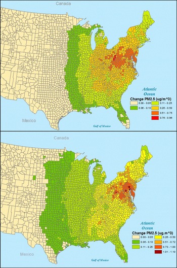
Difference in PM2.5 concentrations between no-scrub counterfactual and observed emissions of SO2 for 2008 (top panel) and 2011 (bottom panel).

The top panel of Figure 4 further concretizes the benefits reported in Table 1 by mapping the change in ambient PM2.5 in 2008 estimated to result from FGD units installed between 2005 and 2008. The map focuses on the eastern two thirds of the United States because the vast majority of units were installed in the east. The greatest reduction in PM2.5 concentrations occurred along the Ohio River near the tristate convergence of Ohio, West Virginia, and Pennsylvania. In this small zone, PM2.5 annual average concentrations fell by between 0.75 ug/
 $\text{m}^{3}$
and 0.95 ug/
 $\text{m}^{3}$
. The connection to Table 1 is clear in that Ohio, West Virginia, Pennsylvania, and Kentucky (also adjacent to the zone with large PM2.5 reductions) were all among the states that experienced large benefits from SO2 reductions. Figure 4 also shows an area of considerable PM2.5 reductions (between 0.5 ug/
 $\text{m}^{3}$
and 0.75 ug/
 $\text{m}^{3}$
) extending eastward through southern Pennsylvania, Maryland, and Virginia. Further, some of the large eastern metropolitan areas lie within a zone of PM2.5 reductions in excess of 0.5 ug/
 $\text{m}^{3}$
. This occurs because the prevailing east–west wind direction translates abatement in the Ohio Valley into PM2.5 reductions along the East Coast.
The bottom panel of Figure 4 maps ambient PM2.5 concentrations in 2011 due to the installation of FGD units between 2008 and 2011. Differences in concentrations between the observed emission case and the no-scrub counterfactual are generally increasing from west to east, with the greatest change in concentrations in the Mid-Atlantic States. Two aspects of the bottom panel of Figure 4 are worth noting. First, the maximum change in PM2.5 is larger than in 2008. There are a few counties in and near large cities with changes in PM2.5 levels over 1 ug/
 $\text{m}^{3}$
. Second, the counties that show differences in PM2.5 concentrations of between 0.75 ug/
 $\text{m}^{3}$
and 1 ug/
 $\text{m}^{3}$
tend to lie further to the east than those in the top panel of the figure, and, therefore, in closer proximity to the large eastern metropolitan areas.
Figure 5 completes the modeling exercises by mapping the change in monetary damage, the GED, due to the PM2.5 reductions shown in Figure 4. Because the GED is dominated by human health effects, large cities (within the areas where PM2.5 changes) exhibit the greatest impacts of scrubbing. The top panel of Figure 5 indicates that the large cities along the eastern seaboard incurred significant reductions in damage due to FGD units installed between 2005 and 2008. Counties within each of these major metropolitan areas experience benefits in excess of $100 million. Moving westward, cities in the industrial Midwest, in closer proximity to plants with large emission reductions, also show significant benefits. These include Pittsburgh, Cleveland, Columbus, and Detroit. Further to the west, Chicago also falls into the top benefit category. In the southern states, no counties incur changes in damages in excess of $100 million.Footnote 10
The bottom panel of Figure 5 displays the change in GED in 2011. Relative to the change in damage in 2008, the bottom panel of Figure 5 indicates that most of the counties in and near large eastern cities incur changes in damage in excess of $100 million. In addition to having large exposed populations, recall from Figures 3 and 4 that plants in or nearby to these areas adopted scrubbers, and that many of these counties also experience significant changes in PM2.5. Some of the same metropolitan areas in the Midwest as shown in the top panel of Figure 5 also display large reductions in damages including Pittsburgh, Cleveland, Detroit and Chicago. And in the southern states, metropolitan areas in North Carolina and Georgia incurred changes in damage in excess of $75 million.
Difference in monetary damage between no-scrub counterfactual and observed emissions of SO2 for 2008 (top panel) and 2011 (bottom panel).

Summarizing the figures, the depiction of emission changes corresponds directly to the states showing large benefit-cost ratios, and large absolute benefits, in Table 1, especially those along the Ohio River. Given prevailing wind direction, the resulting reduction in ambient PM2.5 is largest to the east of power stations that installed scrubbers. Namely, along the Mid-Atlantic states and the eastern seaboard. Finally, since the majority of monetary damage from exposure to PM2.5 is due to premature mortality, the greatest benefits from reductions in ambient PM2.5 occur in large cities. As discussed below, this has important implications in terms of the distributional effects of scrubber installation.


3.1.1 Integration of BCA with Augmented National Accounts
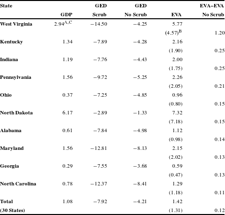
Table 2 reports, for all sectors, aggregate state GDP, GED, and EVA growth rates between 2005 and 2011. (The levels of each of these macroeconomic indicators are reported in the appendix in Tables A.3 and A.4.) The states are ranked in descending order of the spread between EVA growth rates, with-and-without FGD technology adopted between 2005 and 2011. That is, the states in Table 2 are those for which the installation of scrubbers makes the largest impact on growth rates of the EVA measure. Note that abatement costs are added back to market GDP under the no-scrub counterfactual. This assumption will, all else equal, diminish the difference between EVA growth in the observed and counterfactual cases.
Figures 3–5 show that a considerable portion of scrubbing technology was installed at plants in states in the Ohio River Valley. As such, it is not altogether surprising that these states show the largest effect of scrubbing adoption on EVA growth rates. Even when compared to other states along the Ohio River that exhibit large differences in the observed and counterfactual EVA growth rates, West Virginia is an outlier. With FGD technology, West Virginia EVA expanded at an annual rate of 5.77% between 2005 and 2011. Without scrubbers, state EVA would have grown by 4.57%. The difference in augmented growth rates is, therefore, 1.20%, which is much greater than the average over the 30 states that installed scrubbers between 2005 and 2011. This spread is nearly five times larger than the difference in EVA growth estimated in Kentucky and Indiana. The differences in EVA growth rates in Pennsylvania and Ohio are about six and eight times smaller than that of West Virginia, respectively. The large difference in EVA growth in West Virginia stems from the significantly smaller reduction in GED: damages dropped by 14.5% annually with FGD technology and 4.3% without the installed scrubbers. It is also instructive to compare EVA to GDP growth. With FGD technology, EVA growth outpaced market GDP growth by over 2% points. Without new FGD units, EVA growth exceeded GDP growth by just over 1% point.
As mentioned above, Indiana, Kentucky, Pennsylvania, and Ohio – each with more than one facility that adopted new scrubbers during this time period – show large reductions in emissions from FGD use. These states show similar differences in state EVA growth between the observed and counterfactual cases. The differences are between 0.15% and 0.25%. With installed scrubbers, GED in these states dropped by between 7% and 10%, annually. Without FGD technology, GED is estimated to have fallen by between 4% and 5%. Notice that GDP growth in these states was quite sluggish; only Pennsylvania grew by more than 1.5%, annually. During the later years of the sample, these manufacturing-based economies were exhibiting effects of the Great Recession. In these states, the EVA growth rates were between 1.5 and 2 times more rapid than GDP growth.
One central takeaway from Table 2 is that EVA in Rust Belt states, even in the no-scrub counterfactual, provides a very different portrayal of performance relative to market GDP. Second, investments in environmental quality, when properly accounted for, had an appreciable and positive effect on output growth among states in this region.
Outside of the Rust Belt, North Dakota experienced rapid growth in market output between 2005 and 2011. North Dakota GDP expanded by 6.2% annually. Much of North Dakota state product over this time period was comprised of oil and gas extraction. Concurrently, state GED fell at a more modest rate than the other states in Table 2. With new FGD units state GED fell by about 3%. In the no-scrub counterfactual, GED would have fallen by only 1.3%. Further, North Dakota’s EVA growth rate between 2005 and 2011 was 7.3%. Counterfactual EVA expanded at a 7.2% rate. Relative to Rust Belt states discussed above, in which EVA growth was 1.5 or two times greater than market growth, in North Dakota, EVA growth was only incrementally greater than GDP growth.
The state economies of Alabama, Georgia, and North Carolina each expanded at rates below 1% from 2005 to 2011. Observed EVA growth was nearly double GDP growth in Alabama and Georgia, and about one and two thirds more rapid than market growth in North Carolina. Again, the EVA measure, which captures the return to public investments in air quality, provides a very different sense of economic performance over this time period than a metric such as GDP which omits benefits from scrubber use than manifest outside the market boundary.
In total, for the 30 states that put FGD units in place between 2005 and 2011, the difference in EVA growth with-and-without scrubbing was 0.12%. This difference was driven by the fact that GED fell by 8% annually with scrubbing, and by 4% in the no-scrub counterfactual. Importantly, adoption of FGD units is estimated to have enhanced state growth between 2005 and 2011, provided output is measured in a manner that is inclusive of both the benefits and costs of scrubber adoption. The difference between EVA and GDP growth in aggregate across all states was about 0.34%.
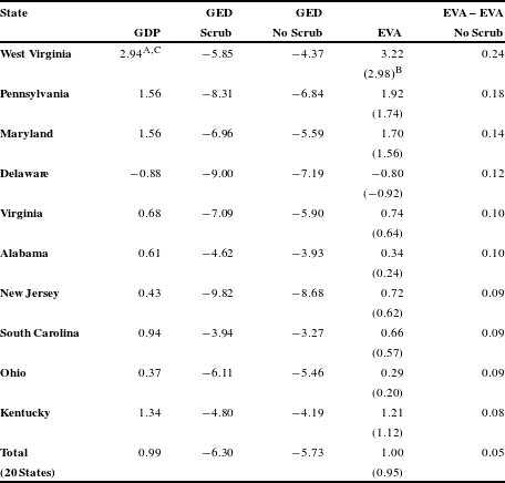
Table 3 employs a different measure of the benefits from scrubber adoption. Throughout the analysis thus far, GED measures damages caused by emissions produced in a state. Calculated in this way, the GED are inclusive of impacts that manifest within the emitting state and in other downwind states. In contrast, Table 3 calculates the GED in terms of where exposures and damages occur and then totals up GED by state of occurrence, irrespective of where emissions are produced. This tack to tabulating GED perhaps provides a more direct link to state welfare as it relates to pollution exposure.
Growth rates of GED, EVA, and GDP between 2005 and 2011 Computed Using States as Receptors.


Table 3 shows that using the alternative approach to measuring GED has mixed results in that some states’ indicators are quite sensitive to this different method while others are not. States located in the Ohio River Valley such as West Virginia, Ohio, Pennsylvania, and Kentucky retain large differences in EVA rates (and hence appear in both Tables 2 and 3). Maryland and Alabama also show up in both tables. The four states in Table 3 not in Table 2 are: New Jersey, South Carolina, Virginia, and Delaware. It is revealing that all of these states lie on the eastern seaboard. GED attributed to emission changes in these states are likely to have a small effect on EVA growth because a nontrivial share of emissions harmlessly drifts over the Atlantic Ocean. In contrast, GED calculated as exposures in these states are sensitive to changes in scrubber use at power stations throughout the Midwest and eastern United States. With significant changes in GED that occur in these states (because of substantial upwind abatement) the difference between observed and counterfactual EVA growth rates is large, as indicated in Table 3.
The finding that the difference in EVA growth rates from scrubbing adoption is largest in West Virginia is robust to whether GED is measured using the location of exposure or emissions. The difference is about 0.25% in Table 3 and when the GED is measured as the damages caused by emissions produced in West Virginia, the spread in EVA growth rates from scrubber adoption was 1.20%. In West Virginia, the exposure-based GED fell by 5.85% with scrubbers and by 4.37% in the no-scrub counterfactual. Table 2 reported that the emission-based GED fell by 14.5% in West Virginia with FGD, and it declined by 4.25% in the counterfactual. The more pronounced reduction in GED when counted according to emissions released in the state translates through to a more pronounced effect on EVA growth rates.
Some of the states in Tables 2 and 3 have similar differences in EVA growth rates regardless of whether the exposure-based or the emissions-based GED is employed. For example, Pennsylvania shows a difference of 0.21 in Table 2 and 0.18 in Table 3. In contrast, the spread in EVA growth rates for Kentucky was 0.25 in Table 2 and just 0.08 in Table 3. Consider that Pennsylvania lies both downwind from many coal-fired power plants that installed scrubbers (in Ohio, Kentucky, and Indiana). However, Pennsylvania also has a large in-state population, and is upwind from large metropolitan areas on the Eastern seaboard. As such, the GED computed for Pennsylvania change at similar rates (across the observed and counterfactual emission scenarios) whether the exposure or emission-based GED is employed.
In contrast, Kentucky is rural, with a small in-state population. It lies upwind from the major population centers on the East Coast, but tends not to import pollution from Ohio and other Midwestern states. As such, the GED computed using the emissions (which is inclusive of out-of-state damages) fell at an 8% rate, whereas the GED calculated using in-state exposure only declined by 4.8%, annually. Coupled with the fact that the GED under the no-scrub counterfactual declined by similar rates irrespective of how GED was tabulated, the EVA rate spread in Kentucky was much smaller when the exposure-based GED is employed.
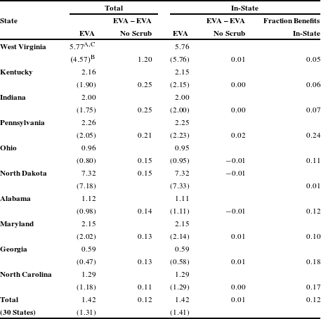
EVA Growth between 2005 and 2011 with In-State Benefits.


Table 4 attributes the GED back to the location of emission, however it restricts the analysis to benefits that manifest within the state where FGD units were installed. Figure A.1 in the appendix displays the key parameter driving the results in Table 4 – the share of benefits that manifest in-state. The map clearly indicates that Florida and Texas retain the largest share of benefits in-state. Broadly, more populous states tend to reap a larger share of benefits than more rural states. As such, Pennsylvania, Maryland, Virginia, and Ohio (among others) retain between 10% and 25% of benefits within-state borders. Indiana and Michigan retain smaller shares despite having large cities within their borders. These smaller shares stem from the fact that FGD units were installed on plants that are near their borders with downwind states. More westerly states (Wyoming, North Dakota, for example) show very small shares of in-state benefits because of low population density.
The bottom row of Table 4 indicates that, when the analysis is limited to just “in-state” benefits, the difference in EVA growth with-and-without FGD installation falls to 0.01% (from 0.12%). Nearly all of the difference in EVA growth rates is eliminated when examining only within-state effects. Hence, most of the EVA growth boosting effect of FGD installation manifests in benefits across state boundaries. This reduction is especially prominent in the ten states listed in Table 4. For example, including interstate benefits, FGD units installed in West Virginia increased EVA growth by 1.2%, as reported in Table 2. Limiting the calculation to in-state benefits yields an increase of just 0.01%. This result stems from the relatively large export share for West Virginia (see Figure A.1). For Pennsylvania, which retains 24% of benefits in-state, the EVA growth effect of scrubbing is just 0.02%, relative to 0.21% including interstate benefits.
North Dakota is an interesting case. For North Dakota, the gap between EVA growth in the observed and counterfactual cases was 0.15%. Restricting benefits (reduced GED) to that which occurred in North Dakota changes the sign of the difference in EVA between the observed and counterfactual contexts. Thus, when only counting in-state benefits, EVA would have expanded more rapidly without scrubbing in North Dakota. This result manifests because nearly all of the benefits materialize outside of North Dakota. However, the full abatement costs of scrubbers are attributed back to the North Dakota economy. In the restricted in-state accounting experiment, there is no, or very little, boost because the majority of benefits are out of state. All that is left in the augmentation are abatement costs, which under the counterfactual are added back to state GDP. As a result, the no new FGD counterfactual yields higher growth than the observed case. A similar phenomenon manifests in Alabama and Ohio. Figure 3 indicates that the power stations in Ohio that added FGD units are clustered along the state border; a large share of emissions exits the state and the benefits of abatement manifest elsewhere. A like pattern is evident for Alabama.
To summarize Table 4, focusing just on in-state benefits drastically reduces the difference in EVA growth rates between the observed case and the no-scrub counterfactual. From the perspective of a state regulator, the results in Table 4 are those that are most tangible. Recall the discussion from Section 1 regarding the interpretation of state and regional accounts. GED is deducted from GDP to estimate EVA. Abatement is reflected in higher EVA growth because (unpriced) costs, the remaining GED, fall. Here is the cautionary note from Section 1; although EVA growth increases due to abatement in a particular (emitting) region, the physical benefits manifest in other regions. This is a function of how the air pollutants, SO2 in particular, move through the atmosphere and it is also related to the location of specific plants within states. The result is that a state regulator with a more limited objective function (only in-state benefits matter), will consider GED reductions from abatement that are much smaller in magnitude than the (interstate) total benefits.
This finding has important implications with respect to the design of an augmented accounting regime such as the EVA. Clearly a federal regulatory body is the appropriate institution to design and implement such a system. The interstate flow of air pollution suggests that a considerable share of benefits from installing abatement technology manifest across state lines. A myopic state regulator would have no incentive to build such effects into a state-based EVA. And, as shown in Table 4, the growth effects of scrubber installation would be miscalculated to a considerable degree.
The results presented in Table 4 also suggest that state regulators, perhaps also elected officials, may have differential preferences over environmental policy depending on the share of benefits that accrue within their state borders. As Figure A.1 and Table 4 indicate, the in-state share of benefits depends on population density and the location of facilities conducting abatement. Given local knowledge of these factors, local regulators are likely to have preferences that align with federal policy when such policies target facilities that produce in-state benefits. Conversely, state regulators are more likely to resist federal policies that predominantly yield out-of-state benefits. Of course, the manifestation of costs from policy is also an important factor driving state and local regulators’ preferences.
3.2 Incidence of Benefits by Income and Demographics
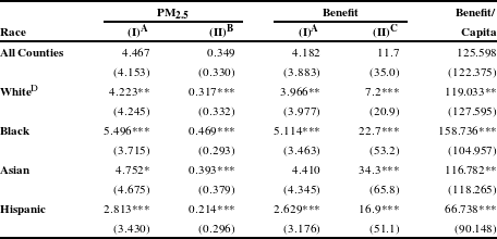
Table 5 reports changes in ambient pollution concentrations and monetary benefits by the racial characteristics of exposed populations. In all counties, PM2.5 concentrations were estimated to be 4.5% higher under the counterfactual. This amounts to a difference of about 0.35 ug/
 $\text{m}^{3}$
. Counties with a large share of African Americans experienced the largest absolute and percentage reduction in PM2.5 (both changes are significantly different from the change in all counties at the 0.01 level). Counties with large Asian populations also incurred relatively large reductions in PM2.5, though the percentage change is only marginally significantly different from the change in all counties. Among populations with greater than average shares of white and Hispanic persons, the reductions in PM2.5 were lower, and significantly different from the all counties change. Intuitively, the same pattern holds for monetary benefits of abatement due to FGD unit installation. The largest percentage change in monetary damages manifests in counties with greater than average shares of African American populations. The only change in damages among demographic categories that is statistically indistinguishable from the all counties case is the percentage change in benefits among counties with large Asian populations.
Benefit Incidence and County Demographics: 2011.

A
 $=$
Columns (I) show percentage change.
B
 $=$
Column (II) for PM2.5 shows change in ambient concentration (ug/
 $\text{m}^{3}$
).
C
 $=$
Column (II) for benefits shows change in damage, or benefit in ($ millions).
D
 $=$
Distinctions by race show results for counties with fraction of each ethnicity above the national mean fraction for that ethnic group.
T-tests for comparison of means relative to “All-County” means. *
 $=$
difference significant at 0.10; **
 $=$
difference significant at 0.05; ***
 $=$
difference significant at 0.01.
The final column in Table 5 reports the benefits on a per-capita basis. Across all counties, the benefits per capita were estimated to be $125. Among counties with larger than average population shares of African Americans, benefits per capita were over $158. All three of the remaining race categories show benefits per capita that were lower than the all-county results. In particular, in counties with a larger than average share of Hispanic persons, the benefits per capita were calculated to be just $67. Figure A.2 displays the benefits (or the change in damage) per capita, by county in 2011. Many areas in the states of Pennsylvania, Maryland, and West Virginia incur benefits in excess of $200/person. Counties with the largest per-capita benefits tend to be those in rural locations in these three states. Note that all of the race-specific decompositions of benefits per capita are statistically distinct from the all-county results.
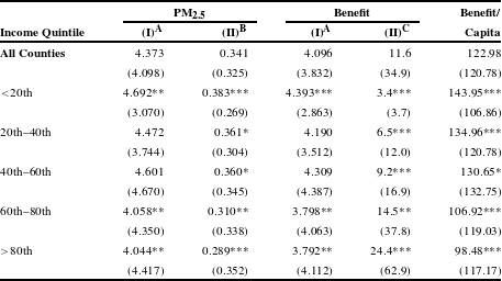
Benefit Incidence and County Per-Capita Personal Income: 2011.

A
 $=$
Columns (I) show percentage change.
B
 $=$
Column (II) for PM2.5 shows change in ambient concentration (ug/
 $\text{m}^{3}$
).
C
 $=$
Column (II) for benefits shows change in damage, or benefit in ($ millions).
T-tests for comparison of means relative to “All-County” means. *
 $=$
difference significant at 0.10; **
 $=$
difference significant at 0.05; ***
 $=$
difference significant at 0.01.
Table 6 displays the benefits of FGD adoption according to income quintiles, by county. The greatest percentage changes in PM2.5 concentrations occurred in counties toward the bottom end of the income distribution. For example, in counties below the 20th percentile, the reduction in PM2.5 was about 4.7%, whereas the change across all counties was estimated to be 4.4%. In contrast, counties at or above the 60th percentile experienced reductions in PM2.5 below the 4.4% all-county average. While percent changes in PM2.5 below the 20th percentiles and above the 60th percentiles are statistically distinguishable from the all-county change, PM2.5 perturbations in counties from the 20th percentile to the 60th percentile are not statistically different from the all-county change. The benefits per capita are largest in counties with incomes below the 20th percentile and the benefits per capita fall monotonically through the income distribution. For counties with income above the 80th percentile, benefits per capita are estimated to be about $100. This is about 30% smaller than the per-capita benefits that manifest in the lowest income counties. While the magnitude of these monetary benefits is small (less than 1% of incomes in each quintile), these results suggest that the installation of scrubbers generated improvements in public health that were progressively distributed across populations of different incomes.
3.3 Sensitivity Analysis
Table A.1 displays the first set of results from the sensitivity analysis. In particular the table reports the benefit-cost ratios (using the high abatement cost approach) for scrubbers installed between 2005 and 2011. Broadly, the rank ordering of states according to the largest benefit-cost ratios is quite robust across the three different modeling approaches. The states that populate the table are the same across modeling tacks. The present discussion focuses on West Virginia both in the interest of brevity, and given the dramatic effect of FGD investment on EVA growth rates in that state. Using the default modeling approach, FGD units installed in West Virginia between 2005 and 2011 generated a benefit-cost ratio of 27:1. However, this ratio increases to 43:1 when using the PM2.5-mortality dose–response function published in Roman et al. (Reference Roman, Walker, Walsh, Conner, Richmond, Hubbell and Kinney2008). Note that the mortality coefficient reported in Roman et al. (Reference Roman, Walker, Walsh, Conner, Richmond, Hubbell and Kinney2008) is about 60% larger than that found by Pope et al. (Reference Pope, Burnett, Thun, Calle, Krewski, Ito and Thurston2002) which is employed in the baseline case. The ratio is estimated to be 11:1 conditional on a $2 million VSL (which is one third of the magnitude of the default $6 million VSL). A review of the remaining nine states in Table A.1 reveals that the benefit-cost ratios range between 53:1 and 37:1 when the alternative dose–response function is employed. Similarly, the ratios extend from 13:1 down to 9:1 when the VSL parameter is set to $2 million VSL. Hence, these two important modeling parameters have a transparent influence on the estimated benefit-cost ratios.
Table A.2 reports the effect that modifying the dose–response and VSL parameters has on EVA growth rates. Under the default assumptions, state EVA increased by 1.20% points more rapidly due to scrubber installation in West Virginia. This spread increases to 1.95% using the alternative dose–response function (Roman et al., Reference Roman, Walker, Walsh, Conner, Richmond, Hubbell and Kinney2008). The difference in EVA falls to 0.45 conditional on the $2 million VSL. The responsiveness to the different modeling assumptions of the spread between EVA growth with-and-without new scrubbers across the remaining nine states in Table A.2 follows from the difference in the magnitude of the alternative parameters. That is, for the $2 million VSL, the difference in growth rates is roughly one third that estimated using the default $6 million VSL. And, using the larger Roman et al. (Reference Roman, Walker, Walsh, Conner, Richmond, Hubbell and Kinney2008) dose–response parameter, the gap between EVA growth rates is greater by roughly one half than under the default assumptions. As was the case for Table A.1 these patterns generally demonstrate the relationship between alternative integrated assessment modeling assumptions and the primary results of the present paper.
4 Conclusions
This paper demonstrates a new synthesis between empirical BCA and the NIPAs. This conflation relies on the estimation of EVA, an augmented measure of output, defined as market output less external environmental damage. The motivation for the exercise is three fold. First, measurement of economic performance during macroeconomic shocks is especially important. Second, comprehensive measurement should encompass private sector output and the consequences of public sector interventions both within and beyond the market boundary. Third, evaluation of public policy, especially in terms of consequences on growth, must rely on a metric of growth that is inclusive of both benefits and costs. This latter point is paramount in the context of environmental policy since a significant share of benefits may manifest outside, or external to, the market boundary. Thus, relying on a market index could yield a potentially biased picture of policy outcomes. The BCA in this paper zeros in on adoption of FGD technology at power plants in the United States between 2005 and 2011. This time period was characterized by rapid accumulation of abatement capital because of anticipated changes in the Clean Air Act relevant to fossil fuel-fired power plants.
The empirical BCA results for the period from 2005 to 2011 indicate that new scrubbing technology produced about $30 billion in net benefits and prevented about 5500 deaths. The benefit-cost ratio across the 30 states that adopted new FGD units during this time period ranges between 20:1 and 53:1. Further, EVA grew 0.12% more quickly with FGD units than without in these 30 states. While most abatement occurred at power plants in the Rust Belt and the Southeastern states, the benefits tend to manifest in cities along the East Coast. Because of this, attribution of out-of-state benefits to the power plants that installed scrubbers is essential in tracking the EVA. The paper shows that the vast majority of benefits manifest in different states than where technology is deployed, and that an EVA metric that only encompasses in-state benefits is a grossly biased augmentation to GDP.
The sample integration of environmental BCA with the NIPAs provides evidence that environmental policy may have an appreciable, positive effect on augmented measures of output and growth. This finding stems from the inclusion of monetary benefits directly into the EVA metric. Second, the particular context explored herein is characterized by significant spatial heterogeneity; for a few states (West Virginia, for example) integrating BCA with state output has a dramatic effect on augmented state growth. Importantly, it is critical to re-emphasize that the present paper is not proposing EVA as a welfare measure. Rather, the manner in which EVA adjusts GDP moves the index toward a comprehensive welfare measure. This paper focuses on showing the potential importance of using an index inclusive of both the benefits and costs of environmental policy, especially with respect to calculating the impact of policy on growth.
The BCA framework used herein is explicitly partial equilibrium. The model assumes no general equilibrium effects on labor markets either due to a reduction in the time endowment from excess mortality incidence or due to the decrease in the capital stock from investment diverted to pollution abatement technology. That the model used herein does not encompass, or cannot weigh in on, the jobs-environment tradeoff is especially important given that the period under examination includes the Great Recession. It is during such adverse shocks that policy-induced job loss may be more than transient (Haveman & Weimer, Reference Haveman and Weimer2015). The paper also does not model the effects of abatement technology on electricity prices or the prices of other goods in the economy that would be affected by power prices.
In order to assess what these omissions mean for the BCA conducted here, especially on the cost side of the ledger, the general equilibrium analysis conducted by the USEPA (2011a ) is helpful. The USEPA (2011a ), reports that, in 2010, the entire Clean Air Act lowered GDP and consumption by about 0.5%. The reduction in GDP amounts to an increase of between 50% and 70% over estimated direct compliance costs. For purely illustrative purposes, let us assume that the general equilibrium effects in the present analysis would affect costs by 70%. Then, under high cost case, total costs would rise to $2.7 billion (from $1.6). Net benefits would be $29.6 billion rather than $30.7 billion. The benefit-cost ratio would fall to 11:1 from 19:1. Importantly, the USEPA’s (2011a ) analysis corresponds to the entire Clean Air Act. The present study focuses on abatement technology adopted by one subsector (coal-fired power plants). USEPA estimates that the Clean Air Act reduced mortality incidence by 160,000 deaths in 2010 (valued at $1.2 trillion), whereas the present paper considers a policy intervention that avoids 5500 deaths. Together with the back-of-the-envelope calculation above, it is unlikely that the partial equilibrium approach, while incomplete by construction, omits large general equilibrium costs.
While the preceding paragraph compares the partial and general equilibrium cases empirically, a conceptual comparison is also useful. The approach to benefit estimation adopted in the present study shares a key similarity with traditional macroeconomic approaches to policy evaluation. Namely, macro policy evaluations tend to assume that all individuals share a commonly specified utility function (Rogerson, Reference Rogerson2015). Hence, all individuals share common preferences over mortality risk-money tradeoffs. This implies a uniform VSL – an assumption made in the present paper.Footnote 11 A key distinction is that standard macroeconomic policy evaluations allow investment in pollution control technology to reduce the size of the capital stock, which, in turn, reduces producer’s derived demand for labor and wages. Ultimately, raising the cost of capital leads to a lower amount of capital in a policy steady state (Rogerson, Reference Rogerson2015). The model employed in the present paper is not equipped to link technology (FGD) adoption into effects on the conventional capital stock or labor markets. While this is a clear shortcoming of the present analysis, USEPA’s (2011a ) results suggest that these effects are small in magnitude for the policy considered herein.
A few additional caveats to the results presented above are worth pointing out. First, benefits are sensitive to assumptions in the IAM. While the paper explores a few alternative approaches to benefit measurement there are two potentially important issues not directly addressed. One of these is statistical uncertainty in the benefits estimates. That is, parameters such as the VSL and the dose–response function are uncertain. As such, a Monte Carlo analysis is the proper tool for exploration of statistical uncertainty in the benefit estimates. An exercise of this type is a possible extension of work conducted herein. And finally, model uncertainty is not treated. That is, repeating the exercise with a different IAM would provide a sense of whether the key results reported herein are in some way a function of the approach to benefit measurement used in this paper.
Supplementary material
To view supplementary material for this article, please visit https://doi.org/10.1017/bca.2017.15.