Prominent among the term-paper topics for W. A. Lewis's graduate economic history seminar at Princeton was “The peopling of Malaya.” Certainly Malaya was remarkable enough to merit such attention. Nor was it the only Southeast Asian country that, as part of a late nineteenth- and early-twentieth-century process of rapid globalization, was the recipient of mass immigration. Although only a handful of Europeans went to Southeast Asia, the region, reflecting its location on the main east-west shipping route, was the principal destination of the world's other two pre–World War II mass emigrant flows. These were from India and China.
Writing about late-nineteenth- and early-twentieth-century globalization, Lewis spoke forcefully of the “unlimited supply of Indians and Chinese willing to travel anywhere to work on plantations for a shilling a day.”1
Lewis, Evolution, p. 15.
On the late nineteenth-century creation of global factor markets, see Williamson, “Land, Labor,” which (p. 82) specifically draws attention to “Lewis's grand Third World research agenda.” On Asian commodity market integration, see Latham and Neal, “International Market,” pp. 260–80; Brandt, “Chinese Agriculture,” pp. 169–77; and Commercialization, pp. 16–25.
Harley, “Review,” p. 928.
Before the Second World War, large voluntary migrant flows to Southeast Asia led some commentators to state what became the labor supply basis of the Lewis hypothesis. Singapore, a European resident wrote in 1931, is near “two unlimited sources of supply for cheap labour, namely India and China.”4
Rotary Club, Singapore, p. 2.
Bernardelli, “New Zealand and Asiatic Migration,” p. 41. Bernardelli lived in Burma before the Second World War and wrote an appendix to the 1941 Report on Indian Immigration. Observers of other Southeast Asian countries paint a similar picture, especially after the turn of the century, of largely free labor markets and highly mobile immigrant labour. See Vlieland, “Population,” p. 66; Bauer, Rubber in Malaya, pp. 217–18; and Feeny, “Extensive versus Intensive,” p. 697.
Diaz Alejandro, Essays, pp. 21–22.
Leff, Economic Structure, pp. 63–71.
Recently, a literature, identified as “revisionist” by its authors, has questioned what it describes as “immigrant-augmented elastic labor supplies.”8
The two quotations are from Williamson, “Real Wages, Inequality,” p. 123. For this revisionist literature see also Williamson, “Globalization, Factor Prices,” pp. 22–23, 33–38; O'Rourke and Williamson, Globalization, pp. 139–41; Taylor, “Mass Migration,” pp. 94–97, 109; and Hatton and Williamson, “Latecomers,” pp. 55, 69; Age of Migration, p. 44, and Global Migration, pp. 68–70. Although the concept of unlimited labor and a resulting constant real, unskilled wage is almost universally associated with Lewis, it can be shown that wage constancy need not arise from unlimited labor. Kelly and Williamson, “Writing History Backwards,” pp. 733, 739, 769–74. However, Ranis, citing the work of Sen, observes that neoclassical explanations and horizontal labor supply curves do not easily fit together: “you have to work hard to make the preconceived theory fit the facts.” “Is Dualism,” p. 11.
O'Rourke and Williamson, Globalization, p. 141.
Williamson, “Globalization, Factor Prices,” p. 40.
We find, on the contrary, that Lewis's hypothesis of unlimited labor emerges with a remarkably clean bill of health for Burma, Malaya, and Thailand between the 1880s and World War II. For these three countries, abundant, responsive labor in India and China led to a Lewisian long-term horizontal labor supply curve. In conjunction with globalization and mass migration within Asia, an integrated labor market prevailed across an area stretching from South India to Southeastern China. Highly mobile, cheap labor and “vent-for-surplus” opportunities—both in the production for export of primary commodities in Southeast Asia and in the complementary export to Southeast Asia of labor from India and China—were defining features of late-nineteenth- and early-twentieth-century globalization in Asia and its integration into the world economy.
TRADE AND IMMIGRATION IN SOUTHEAST ASIA
Vent-for-Surplus Trade
By the 1880s Western industrialization and a communications revolution, including the opening of the Suez Canal and adoption of steamships, created a new demand for products that Burma, Malaya, and Thailand could produce on vast amounts of unused land. International trade provided the “vent” or outlet to utilize surplus Southeast Asian natural resources in the production of commodities that, unless exported, would not have been worth the effort of producing. Vent-for-surplus models vary. They may involve only land or other natural resources without alternative uses and which cannot be switched to domestic use.11
Caves, “‘Vent for Surplus’ Models.”
Myint, “Gains” and “‘Classical’ Theory”; and Findlay, Trade, pp. 70–74.
Adas, Burma Delta, p. 59, see also p. 26.
Ingram, Economic Change, p. 54.
In the three Southeast Asian countries vent-for-surplus trade led to dramatic export expansion and specialization in a few primary commodities. Exports from the three countries, expressed in 1913 U.S. dollars, increased from $59.5 million in 1871–1873 to $919.9 in 1936–1938, equivalent to 4.2 percent annual average growth. Rice comprised the bulk of exports from Burma and Thailand, and in both was grown by small farmers. In Malaya tin mining developed in response to the late-nineteenth-century innovation of tinned food in the West and until about 1910 remained a highly labor-intensive and largely Chinese industry. Starting in 1905 the spread of rubber cultivation, almost entirely due to the need for rubber tires for automobiles, gave Malaya what soon became its chief staple. Tin and rubber exports from Malaya went almost exclusively to the world economy's industrial core, especially the United States. Burma and, even more, Thailand were increasingly connected to the Malayan economy, which they supplied with rice.
Immigration to Southeast Asia
Export expansion on the scale of Southeast Asia's, involving little, if any, technical change in agriculture, soon necessitated much larger inputs of labor than were available in Southeast Asia itself. The colonial authorities in Burma and Malaya, both under British rule from the late nineteenth century onwards, regarded cheap labor as fundamental to economic growth and strongly encouraged its supply through immigration. In Burma, as a province of India, there were no restrictions on the immigration of Indians until 1938, when Burma became a separate British colony. Immigration to Malaya, apart from temporary controls during the early part of World War I, was unrestricted until the 1930s.15
Malaya, 1921 Census, pp. 21–22; and Purcell, Chinese, p. 203.
Blythe, Methods and Conditions, p. 3.
Skinner, Chinese Society, p. 177; and Landon, Chinese in Thailand, pp. 206–07.
On either side of the Southeast Asian countries—as a near perfect complement to their resource rich but labor scarce factor endowments—geography threw up two exceptionally resource poor but labor abundant and low wage areas: South India and Southeastern China. Between them these areas accounted for the great bulk of Indian and Chinese immigrants to the three Southeast Asian countries. Negapatam, the great port of Tamil emigration from Madras, was only a little over 900 nautical miles from Rangoon, and about half as far again from Penang, the destination for most Indians coming to Malaya. Just west of Southeast Asia lay the provinces in Southeastern China of Kwangtung (Guangdong) and Fukien (Fujian). They were at most 1,500 nautical miles (a journey of no more than about a week) from Singapore and historically had extensive shipping links to Bangkok, either direct or via Singapore.18
Distances are from Philip, ed. Philip's Mercantile Marine Atlas, endsheet table. On Thailand's shipping links see Skinner, Chinese Society, pp. 47–50.
See, for example, India, Census 1901, Madras Report, part 1, pp. 27–32; India, Census 1921, Burma Report, part 1, p. 31, and 1931, Burma Report, part 1, p. 61; Kumar, Land and Caste, pp. 104–05, 144, 161–67; India, Census 1931, Madras Report, part 1, p. 93; and Buck, Land Utilization, pp. 76–77, 125–28.
Burma, Malaya, and Thailand were by no means the sole world outlets for emigration from India and China but they drew a large and increasing proportion of all emigrants from these two countries. Burma received chiefly Indian immigrants and Thailand mainly Chinese. Malaya, about equidistant between China and India, attracted large numbers of both Chinese and Indians.
Immigration data for Southeast Asia come mainly from government reports compiled by port or customs officials. The reports have, on the whole, been judged reliable.20
Sources for all data in the article are given in Appendix 1. A 17-page appendix containing a full discussion of data and sources is available from the authors.
Between 1881 and 1939 Burma, Malaya, and Thailand received over 15 million Chinese and Indian immigrants, more that these countries' total 1881 population (Table 1). During this period, Malaya averaged immigrant inflows per decade of 826 persons per 1,000 resident population, almost five times the immigration rate to Argentina, which had higher rates than any other New World country. Immigrant inflows to Burma and Thailand were on a par with, or above, New World rates. Typically, immigrants to Southeast Asia intended to stay from three to at most five years, and over the six decades in Southeast Asia immigrant retention (net as a proportion of gross immigration) of under a fifth compares poorly with the United States' two-thirds. But in Southeast Asia new arrivals more than replaced departures and, together with greater natural increase, continuously augmented labor supply.

Figure 1 plots gross and net immigration per 1,000 population for Burma, Thailand, and separately for Chinese and Indians coming to Malaya. The trend was upwards. But more striking are the extreme fluctuations in immigration to Southeast Asia. For all three counties the unmistakable impression is of a highly mobile immigrant population alert to economic signals and taking decisions on this basis. Swings in immigration were greatest during the interwar years and the most extreme in Malaya. For that country between 1926 and 1932 the loss of 650,000 persons implied by the drop in immigration rates in Figure 1 was equal to 20 percent of the 1921 population. In Malaya and Thailand gross and net immigration fluctuated similarly and had positive correlation coefficients of 0.82 and 0.79 respectively. The near absence in Burma of correlation between gross and net flows (a coefficient of 0.14) was at least partly due to significant seasonal migration. A first wave of migrants arrived between January and May for the preparation of rice land, mainly the repair of ridges of earth between adjacent fields, before seasonally employed Indians again returned some months later for the harvest.21
Furnivall, “Industrial Agriculture,” pp 95–96.

FIGURE 1 SOUTHEAST ASIA IMMIGRATION RATES, 1882–1939
Methods of Immigration
In the late nineteenth and early twentieth centuries, various forms of slavery, debt slavery and corvée were still present, if with declining incidence, among indigenous Southeast Asians.22
Feeny, “Decline,” pp. 291–95, and “Breaking,” pp. 83–97; and Gullick, Indigenous Political Systems, pp. 98–105.
Skinner, Chinese Society, p. 53; Cheng, Rice Industry, pp. 117–24; Saw, Singapore Population, pp. 46, 48; Sandhu, Indians, pp. 89–108; and Blythe, Methods and Conditions, pp. 91, 97–98.
One major system of immigration in Southeast Asia was personal recruitment, which depended either on individuals returning from the region to persuade others from their home area to emigrate, or on professional recruiters. Personal recruitment, for Chinese known as credit ticket immigration, usually bound the immigrant to specific employment until the debt for passage expenses could be repaid. A well-known feature of emigrant areas in Madras was extreme poverty. For many Indians, emigration with a maistry (experienced Indian worker acting as a labor recruiter) and an associated provision of finance lifted poverty as a barrier to emigration.24
On the historical importance of poverty constraints, see Hatton and Williamson, Global Migration, pp. 43, 48, 58–62, 140, 144.
Adas, Burma Delta, pp. 92, 120.
Furnivall, “Industrial Agriculture,” p. 95.
Credit ticket and maistry systems of immigration were clearly open to abuse. Although not formal indenture, they could be manipulated to create a hold over laborers once in Southeast Asia. Debt incurred for passage, food, and lodging before immigrants started to work might be unreasonably inflated, and when sold on to employers, further increased through the monopoly sale of goods, supply of opium, or rigged gambling games. Abuse remained common and considerable. But its severity, and so accompanying labor tying devices, appear to have lessened markedly by the 1880s in Thailand and Burma, and in Malaya after 1890. Once in Southeast Asia, immigrants who did not themselves pay their passage seem generally to have succeeded in working free of debt. As such they were at liberty to move to other jobs. Even by the late nineteenth century and increasingly thereafter the picture is one of a substantially free Southeast Asian labor market and mobile workforce.27
Bernardelli, “New Zealand and Asiatic Migration,” p. 41; Blythe, Methods and Conditions, pp. 1–3; Andrew, Indian Labour, p. 37; Bennison, Enquiry, pp. 75–80; Skinner, Chinese Society, pp. 53–58; Feeny, Political Economy, p. 163; Cheng, Rice Industry, pp. 123–24; Baxter, Report, p. 75; Vlieland, “Population,” p. 66; Bauer, Rubber Industry, pp. 217–18; Wong, Malayan Tin Industry, pp. 67–76; and Look Lai, “Asian Contract,” pp. 233–35, 256–58.
A second major system of immigration was for those emigrating to Southeast Asia to pay for the journey themselves. For late 1880s Malaya, Wong Lin Ken points to “the increase in the number of immigrants who could pay their own passages, either because they were helped by friends and relatives who already had made some money from the tin mines or elsewhere, or because they were Chinese labourers returning to the Straits to make more money.”28
Wong, Malayan Tin Industry, pp. 66–67.
Adas, Burma Delta, p. 98.
India, Census 1931, Madras Report, part 1, p. 80; and see Madras, Madras Census 1871, p. 75; Bennison, Enquiry, pp. 75, 76, 80.
United Kingdom, Royal Commission on Labour in India, vol. 7, part 2, p. 33 and see p. 39. The speaker, in evidence, was G. T. H. Bracken, District Magistrate and Agent to the Governor, Vizagapatam. See also India, Census 1911, Madras Report, part 1, p. 26.
In 1907 Indian immigration to Malaya, unlike other migrant inflows, began to be organized under government auspices. The rubber industry was just starting and European estate owners and government officials alike were anxious to ensure a supply of cheap labor. In response, the government in Malaya established the Indian Immigration Fund to which all employers of Indian labor (effectively European rubber planters) were obliged to contribute. Immigration from India consisted overwhelmingly of Tamils from the Madras Presidency, and the 1931 census found three-fifths of Malaya's Tamil population to be employed on rubber estates.32
Malaya, 1931 Census, p. 85.
Bauer, Rubber Industry, pp. 220–22; Parmer, Colonial Labor Policy, pp. 38–39; and Saw, Singapore Population, pp.46, 48
Immigrant workers in Southeast Asia were typically able to save and remit money. In China, those returned from Southeast Asia were often distinguished by owing better houses, or by using savings to purchase land or start a business.34
China, Maritime Customs Decennial Reports 1902–11, vol. 2. Southern and Frontier Reports, p. 115; see also 1922–31 vol. 2. Southern and Frontier Reports, p. 153.
Davis, Population of India, p. 104; and United Kingdom, Royal Commission on Labour in India, vol. 7, part 1, p. 295.
India, Census 1931, Madras Report, part 1, pp. 93–94. Tanjore was a coastal district in the Madras Presidency located not too far south of Madras city.
A MODEL OF IMMIGRATION TO SOUTHEAST ASIA
Most immigrants to Southeast Asia had two related objectives. One was to save money for remittances home or to bring back a lump sum; the other to return to India or China after at most three or four years. In Burma the time horizon was frequently even shorter due to seasonal Indian immigration. The model in this section, developed by Timothy Hatton, focuses on the economic motives important to immigration to Southeast Asia and allows account to be taken of its often temporary nature and substantial annual fluctuations.37
See Hatton, “Model of U.K. Emigration” for a full discussion of the requirements of the model and its microfoundations; see also Hatton and Williamson, “After the Famine,” pp. 580–83.
The model, set out in equation 1, has as its dependent variable, M, arrivals in Southeast Asia per 1,000 resident population and so measures immigration in Southeast Asia in the same way as Figure 1.

Immigration (in logs) depends partly on short-term adjustments to changes between the current and previous year in wages (W) and employment (EM), and partly on one-year-lagged log levels in these variables. The size of immigrant groups already in Southeast Asia (MS), transport (TRAS) represented by Southeast Asian shipping freight rates, and a quadratic trend to take account of improved transport technology also appear as independent variables. Because the “pull” of opportunities in Southeast Asia and a “push” from home are not logically separable but contribute to a single decision, wages enter as the ratio of receiving and sending countries, Wr/Ws.
38Gould, “European Inter-Continental Emigration,” pp. 630–34.
Wage data are chiefly, but not exclusively, from government reports and for the most part are new.39
Compilation of all data and its sources are detailed in the appendix available from the authors.
Bennison, Enquiry, pp. 176–81; Andrew, Indian Labour, pp. 226–50; Malaya, Average Prices; Creutzberg, Changing Economy of Indonesia, 5, p. 78 (budget devised by Polak); Indonesia, Central Bureau of Statistics, “Living Conditions”; van Niel, Living Conditions; Runes, General Standards, pp. 19, 21.
Baxter, Report, p. 91, Adas, Burma Delta, pp. 93–94; Hlaing, Study, p. 49; India, Census 1931, India Report, part 1, p. 70: Skinner, Chinese Society, pp. 224–27; Chen, Emigrant Communities, pp. 74–82; and Singapore, Department of Social Welfare, Social Survey, pp. 108–21.
For discussion of the importance of the exchange rate to Chinese immigration, see Malaya, Census 1921, p. 22; and Chen, Emigrant Communities, pp. 74–75.
Emigrants from India and China were almost all unskilled, largely men, and mainly from agricultural areas. Accordingly, for Madras and Southeastern China we use unskilled male, and predominantly rural, wages. A substantial proportion of immigrants to Southeast Asia took rural jobs. Even if immigrants stayed in cities, the importance of primary production in Southeast Asia's vent-for-surplus economies, its labor-intensive character, and well-integrated labor markets made employment in the staple industries typically the dominant influence in setting unskilled wages. Until 1910 Chinese wages in Malaya are for tin mining as the chief source of employment and thereafter for work on rubber estates. Indian wages in Malaya are for unskilled, chiefly plantation labor until 1910, and then for rubber estate employment. Burma wages for 1880–1901 are for agricultural labor and subsequently for coolie labor, predominantly in rice mills. Thailand is an exception both to the use of rural wages and to a new wage series. Wage data for anywhere in pre–World War II Asia must be treated with caution, and information for Thailand is fragmentary, particularly before 1900. We rely on Thai wage data assembled by David Feeny and James Ingram.43
Feeny, Political Economy, pp. 29, 132–33; and Ingram, “Thailand's Rice Trade,” p. 115.
Harvey, Forecasting, pp. 143–47.
Employment enters separately into equation 1 for receiving countries, EMr, and for India and China, EMs. The separation reflects the fact that at home at least some work was likely. In India, as an informed observer explained, “However wretched conditions were in the recruiting districts, the people had the choice of continuing to eke out a living in the fashion of their ancestors.”45
Bernardelli, “New Zealand and Asiatic Migration,” p. 43.
Huff, Economic Growth, pp. 172–75; and Baxter, Report, pp. 51–56.
No more than partial employment data exist for anywhere in Southeast Asia, and for Madras, Kwangtung and Fukien no employment statistics are available. For all areas we use trade statistics to indicate employment. Its fluctuations are, following Hatton and Williamson, proxied by deviations from trend of the log of (in our case) either exports or imports.47
Hatton and Williamson, “After the Famine,” p. 583. Employment series are detrended for all receiving countries where a time trend was found to be significant. This is intended to capture the tendency of migrants to move at times of economic boom in Southeast Asia.
Chain migration, or a “friends-and-relatives” effect in which the existence of immigrants in a country generates further arrivals, is modeled as the term, MS. It measures the stock of Indians or Chinese domiciled in Southeast Asia divided by receiving country population. A friends-and-relatives effect could be thought especially important for Chinese, because, unlike many Indians, they often did not emigrate to specific employment and because of the complex of village, county, and clan ties in overseas Chinese society. As late as 1960 in the United States, for example, well over half of all Chinese could be traced to a single county in Kwangtung province.48
Hsu, Dreaming, pp. 3, 184.
Chen, Emigrant Communities; and Freedman, Chinese Family and Lineage Organization.
The lagged dependent variable Mt−1 has sometimes been interpreted as a friends-and-relatives effect but is perhaps more usefully thought of as adaptive expectations in response to “news” that reached potential immigrants to Southeast Asia through a variety of sources. These included remittances, letters from those in Southeast Asia, and the activities of labor recruiters. Information flows, or this news effect, between the sending regions and Southeast Asia were good because distances were short and shipping connections regular, and because of remittances. A dense network of remittance firms covered Southeast Asia.50
Sugihara, “Patterns,” pp. 262–65.
China, Maritime Customs Decennial Reports 1902–11, vol. 2. Southern and Frontier Reports, pp. 104, 118, 130.
Song, One Hundred Years' History, pp. 67–68.
Huff, Economic Growth, p. 155.
By the 1880s steamships had replaced sailing vessels for the carriage of immigrants, and good shipping existed across Asia. Transport (TRAS) is measured with an index of Southeast Asian shipping freight rates, because all immigrants first reached Southeast Asia by sea. Immigrant shipping fares to Southeast Asia, typically between about half a week's to three weeks' wages of Chinese rubber estate workers in Malaya, were not high. So long as immigrants intended to remain for two or three years, transport costs were small compared to likely earnings.54
For data on shipping fares see China, Maritime Customs Decennial Reports 1902–11, vol. 2. Southern and Frontier Reports, p. 130; Huff, Economic Growth, pp. 154–55; and Skinner, Chinese Society, pp. 62, 65, 66.
Tregonning, Home Port Singapore, pp. 34–36, 53, 149–50; India, Report of the Agent in Malaya, 1931, p. 5; Shein, Burma's Transport, pp. 68–69; Silverstein, “Politics and Railroads in Burma,” p. 82; Federated Malay States Railways, Fifty Years; and Kakizaki, Laying the Tracks.
Empirical Results
We estimate the model in equation 1 separately for each of the four immigrant inflows to Southeast Asia, namely Indians and Chinese entering Burma and Thailand respectively and arrivals of Indians and Chinese in Malaya. First, however, we explore time series properties of the data using the Kwiatowski, Phillips, Schmidt, and Shin (KPSS) and the Elliot, Rothenberg, and Stock DF-GLS tests for unit roots.56
We do not formally test migrant stock for a unit root. By construction, it is a bounded variable that is unlikely to have a stochastic trend and, furthermore, created by linear interpolation. Accordingly, unit root tests are not applicable.
We test for a unit root in immigration, relative wages, employment series, and shipping freight rates. In all cases, the KPSS test cannot reject the null hypothesis of stationarity at 5 percent and the DF-GLS test cannot reject the null hypothesis of a unit root at 10 percent. This latter is comfortably within the 25 percent significance level suggested by Maddala and Kim (Unit Roots, p. 146). For Burma, the KPSS test statistics (5 percent critical values in parenthesis) are: 0.407 (0.463), 0.232 (0.463), 0.248 (0.463) and 0.082 (0.146) for immigration, relative wages, detrended receiving country employment and sending country employment respectively, and the DF-GLS test statistics (10 percent critical values in parenthesis): −1.833 (−1.612), −2.683 (−1.612), −3.189 (−1.612) and −3.9 (−2.89) respectively. For Thailand, the KPSS test statistics: 0.454 (0.463), 0.18 (0.463), 0.114 (0.463) and 0.304 (0.463), and DF-GLS test statistics: −1.642 (−1.613), −1.678 (−1.613), −4.065 (−1.613) and −2.283 (−1.613). For Malaya Indians, the KPSS test statistics are: 0.226 (0.463), 0.113 (0.463), 0.145 (0.463) and 0.082 (0.119) and the DF-GLS test statistics: −2.806 (−1.613181), −3.294 (−1.612), −1.972 (−1.612) and −3.9 (−2.89). For Malaya Chinese, the KPSS test statistics are: 0.099 (0.119), 0.403 (0.463), 0.145 (0.463) and 0.321 (0.463) and the DF-GLS test statistics are: −3.914 (−2.872), −2.226 (−1.613), −1.972 (−1.612) and −2.419 (−1.947). For shipping freight rates, the KPSS is 0.084 (0.463) and the DF-GLS is −3.465 (−1.612).
Table 2 reports estimation results for equation 1. Its double log specification allows interpretation of coefficients as elasticities. In expressing these we follow a tradition in the literature and analyze a 10 percent rather than a 1 percent change in the independent variables. The term for transport costs, as might be expected from the short and relatively cheap journey to Southeast Asia, never attains significance. It is omitted from the table. Values for R2 of two-thirds to over four-fifths suggest that the variables in Table 2 explain most of the variance in immigration to Southeast Asia. Lagged relative wages and, for Chinese especially, migrant stock emerge as key determinants of immigration. The significance of lagged migration at the 1 percent level in three of four instances, and 5 percent in the other, is consistent, in our interpretation of this variable, with the importance of news fed back from Southeast Asia and rapid immigrant adjustment to it.

Compared to lagged migration, appreciably larger coefficients attach to each of the three immigrant streams for which lagged relative wages are significant. For the remaining immigrant flow of Chinese to Thailand, lagged wages are wrongly signed but insignificant. In Malaya, rubber price fluctuations, the most extreme of any of the world's main primary commodities, were reflected in sizeable medium-term wage swings. These, in turn, elicited a large emigrant response. For Chinese a 10 percent rise in relative wages led to a 9 percent increase in immigration and for Indians a more than 10 percent increase. Overall, wage coefficients for India and China support the existence of a flexible labor supply in sending regions such that a small increase in wages brought forth even more immigrant workers.
The significance of migrant stock for Chinese accords with the overwhelmingly literary evidence of that group's propensity for cooperation and the closely integrated nature of overseas Chinese society. Plural societies, like those which became characteristic of Southeast Asia, encompass a variety of racial and ethnic groups that exist side by side but which remain largely separate occupationally, residentially, and socially.58
The term race, although strictly incorrect, is long sanctioned by Southeast Asian usage as a way to refer to Chinese, Indians, and “indigenous” inhabitants of the region. Racial groups typically encompassed a number of ethnic groupings.
Skinner, Chinese Society, p. 179.
Migrant stock is also significant for Indian migration to Burma but not Malaya. For the latter, the explanation for this seeming unimportance of migrant stock is probably that the great majority of Indian workers on Malayan rubber estates, and so most Indians emigrating to Malaya, came as assisted migrants recruited by a kangany. Under these circumstances, Indians emigrated, in a quite real sense, along with their family and friends, because they traveled with someone born in or near their home village, and in the company of others from the same locale.
Studies of immigration often emphasize the importance of receiving country employment, but we find this only for Chinese responsiveness to changed Malayan job opportunities. While in general our results point to wages, not job availability, as the crucial consideration, that finding must in some measure reflect the fact that, for large numbers of Indians, emigration was to more-or-less assured employment, and this made remuneration the chief issue. In Malaya regulation by European rubber planting interests and government to maintain plentiful labor and, insofar as possible, wage constancy is reflected in the significant and large positive relationship between a change of increased Malayan relative to Indian wages and more immigration. For Thailand, however, this relationship, although marginally significant, is negative and a result for which we cannot adequately account.
In the long term all adjustments have occurred: the deltas in equation 1, now equal to zero, disappear and time scripts become unnecessary. Equation 1 can therefore be written as

The long-run multipliers or elasticities are calculated as

where gj is the parameter of interest from equation 1 and g1 is the parameter, lnMt−1. Long-run equilibrium results indicate the percentage change in immigration to which a 10 percent change in the independent variables would ultimately lead. Thailand apart, all wage elasticities are positive and statistically significant (Table 3). Elasticities were highest in Malaya and especially among the Chinese whose responsiveness to wage incentives is well known. For Chinese a 10 percent rise in relative wages led to a 21 percent increase in immigration and for Indians a 17.8 percent enlargement.

GLOBALIZATION, LABOR MARKET INTEGRATION, AND LEWISIAN LABOR
In the development literature the Harris-Todaro and Lewis models remain dominant theoretical formulations of the relationship between wages and immigration. They are, as Kaushik Basu observes, complementary, because the Harris-Todaro construct is “an elaboration of a short-run segment in the Lewis process.”60
Basu, Analytical Development Economics, p. 161. The models are Lewis, “Economic Development”; and Harris and Todaro, “Migration.”
Asian Market Integration
Asian labor markets would be integrated if an equilibrium relationship existed between wages in sending areas and Southeast Asia's receiving countries. An error correction model is used to test whether such relationships existed and, if so, also to find how quickly equilibrium re-asserted itself after a shock. To establish the links between the error correction mechanism and the migration specification in equation 1, we first represent Southeast Asian labor markets in a demand and supply framework.61
Thanks go to an anonymous referee for this formulation and labor market model.
For each of Southeast Asia's receiving countries annual changes in labor demand, ΔLtd, can be written as

where Wr,t is the receiving country wage, Dt and ΔDt are demand shifts in levels and changes respectively, and ut is a random shock.
Changes in Southeast Asian labor supply, ΔL_ts, depended on immigration, Mt, and also on Nt, increases in the domestic labor force


where Ws,t is wage in the sending region wage and et a random shock.
62In equation 4, immigration is expressed as a function of relative wages and demand in the receiving country and not as a function of past migration. This simplification can be considered as a shift from the loop in the migration model in equation 1 to a linear expansion of it.

or

In this error correction model, changes in receiving country wages depend on levels and changes in aggregate demand, domestic labor supply, and an error correction term, (Wr,t−1 − Ws,t−1). Market integration requires a negative, and significant, coefficient, Φ4, on the error correction term. For a negative Φ4, a rise in receiving relative to sending country wages (a positive equilibrium error) leads to downward pressure on receiving country wages in the next period. Conversely, a negative error correction term exerts upward wage pressure. The larger the coefficient, the more rapid is adjustment toward equilibrium.
All four Southeast Asian labor markets have the required negative error correction coefficient (Table 4). For Indians and Chinese in Malaya significance levels are 1 percent and 5 percent respectively, whereas Burma attains significance at just over 5 percent and Thailand at 10 percent. Adjustment toward equilibrium was quickest for Indian immigration to Malaya, as might be anticipated in light of the strong planter-government efforts to promote immigration, and slowest in Thailand. This latter reflected the large number of Chinese employed on projects organized under government or other institutional auspices and rather inflexible wages for such work. To summarize, Asia from South India across Southeast Asia to Southeastern China had an integrated labor market; this integration arose from wage responsiveness.

Southeast Asian Wage Convergence
Immigrants to Southeast Asia had a choice in destinations. Indians could emigrate either to Burma or Malaya and Chinese to Malaya or Thailand. Furthermore, in Malaya job overlaps, including the many Chinese working on rubber estates, and considerable labor mobility allow one to speak, if not of a common Malayan wage, of wage movements fluctuating around the level obtaining for unskilled Indian workers. This level served as a benchmark for all workers in Malaya.63
Malaya, Report of the Labour Department, 1938, p. 39; Soliva, Economic View, pp. 28–30; and Bauer, Rubber Industry, p. 218.
For use of a similar technique, see Michelacci and Zaffaroni, “(Fractional) Beta Convergence.”
Before World War II in all three Southeast Asian countries full convergence was evident. For all wage series apart from Burma we reject nonstationarity at a 99 percent confidence level.65
The ADF test statistics (p-values in parenthesis) are: −1.79 (0.07) for Burma, −3.82 (0.00) for Thailand, −3.28 (0.00) for Malaya Indian and −3.59 (0.00) for Malaya Chinese.
The ADF test statistics (p-values in parenthesis) are: −3.6 (0.00) for Burma, −3.06 (0.00) for Thailand, −2.56 (0.01) for Malaya Indian and −3.98 (0.00) for Malaya Chinese.
Thin data after 1929 make it difficult to account for the somewhat less clear-cut results for the 1930s. But evidence from the whole sample (notably, the strong pairwise convergence in labor markets of like racial composition) does suggest that economic depression may have bolstered an existing tendency to hire according to racial or other discriminatory criteria. If so, this would explain, at least in part, a degree of post-1929 real wage divergence.67
For the pair Burma–Malaya Indians the ADF statistic is −2.28 (0.02) and for Thailand–Malaya Chinese −2.44 (0.02).
Lewisian Labor Supply
Lewis's hypothesis of unlimited labor and a long-term constant unskilled real wage in migrant receiving areas directly confronts the third question of the effect of globalization and associated mass immigration on Southeast Asian labor markets. To analyze this issue of wage constancy we first use wage series for unskilled labor markets in the three Southeast Asian countries to show trends in real wages expressed in 1913 U.S. dollars between the 1880s and 1939 (Figure 2). Prominent in the figure is the largeness of variance relative to trend in wage series. All four labor markets experienced marked downswings, and some sharp spikes, in wages. None of the four show substantial and sustained wage advance. For both Indians and Chinese in Malaya trend was near zero. In Burma and Thailand there is a moderate upwards trend. However, it derives entirely from an end point in the late 1930s; the trend in wages through 1932 is flat (Figure 2A). For both Thailand and Burma the 1930s were an atypical decade. In Thailand, the new 1932 immigrant permit and residence fees together with scope for arbitrary official exclusion discouraged immigration from China with consequent upwards pressure on Thai wages. In Burma a series of anti-Indian riots similarly affected labor inflows from Madras.

FIGURE 2 SOUTHEAST ASIA REAL EXCHANGE RATE ADJUSTED WAGES, 1882–1939

FIGURE 2a BURMA AND THAILAND REAL EXCHANGE RATE ADJUSTED WAGES, 1886–1932
Figure 3 presents a stylized version of the Southeast Asian market for unskilled labor. The distaste of indigenous groups for wage labor is indicated by the figure's steep domestic labor supply curve, whereas the responsiveness of immigrant Chinese and Indian workers to wages and job opportunities in Southeast Asia made labor supply highly elastic along W*. In fact, real exchange-rate-adjusted unskilled Southeast Asian wages, which were around six to seven U.S. dollars, or something over one British pound for a 24-day month, remained close to the shilling a day indicated by Lewis as sufficient to attract Indian and Chinese emigrants. Even if Southeast Asian employers, themselves often Indian and Chinese, were willing to hire indigenous (non-Indian or Chinese) workers there was no reason to pay above the unskilled immigrant wage, W*.68
For a similar argument made for a nineteenth-century Atlantic wage, see Wright, Old South, pp. 71–78.

FIGURE 3 IMMIGRATION AND THE MARKET FOR UNSKILLED LABOR IN BURMA, MALAYA, AND THAILAND
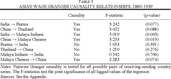
Although labor supply in Figures 2 and 3 conforms to a Lewisian constancy so that no employer in Southeast Asia need worry about bidding up the long-term unskilled wage rate, there is nothing to say that it came about as a result of Indian and Chinese immigration. Granger causality provides a way to try to establish if, as Lewis suggested, international immigration was indeed responsible for the horizontal labor supply curves observed in Southeast Asia. For Southeast Asian labor markets, Granger tests bear out the sequence of change that Lewis indicated (Table 5). Wages in sending regions Granger cause those in Southeast Asia at significance levels of 1 percent for Malayan Indians, 5 percent for Malayan Chinese and 10 percent for both Burma and Thailand.

Granger tests can suggest causality by indicating precedence but they do not guarantee it. In the tests described, however, the likelihood of causation is strengthened because, for three of the four pairings, the possibility of causality from Southeast Asia to India or China can be decisively rejected. In other words, Granger causality is unidirectional. Although the remaining instance of Malayan Chinese does not exclude two-way causation, the statistically more significant link runs from China to Malayan wages. For a pre–World War II labor market stretching across much of Asia, the Lewis hypothesis of unlimited labor fed by mass migration appears to be correct.
CONCLUSIONS AND EXTENSIONS
Vent-for-surplus expansion in late-nineteenth-century Burma and Thailand, as already by the later 1880s in Malaya, would soon have been constrained by lack of labor had these economies been closed to immigration. Accordingly a vent-for-surplus model such as Myint's that encompasses spare labor as well as land requires a geographically Asia-wide formulation if it is to keep touch with the realities of pre–World War II Southeast Asian economic development. In this article we have argued that late-nineteenth- and early-twentieth-century globalization had the effect of creating a highly integrated Asian labor market stretching from South India to Southeastern China, with Southeast Asia at its center. It is illuminating to think of Southeastern China and South India as “hinterlands” of surplus labor sending workers to a “center” of land-surplus Southeast Asia where, in turn, economies were driven by new opportunities for international trade. Over these areas of Asia, surplus natural resources and surplus labor were complementary. Globalization opened the markets that provided an outlet to vent both. In combination with surplus land, Indian and Chinese immigration allowed Southeast Asia's production possibility frontier continuously to shift outwards. This process, together with some imported technology, especially in transport and communications, and the specialization gains associated with Smithian growth, largely provided the basis for economic growth in Southeast Asia.
It is a mistake to think of workers migrating to Southeast Asia as coming from all of India and China because emigration was so heavily from Madras in India and Fukien and Kwangtung in China. In these two Chinese provinces, at any one time a significant proportion of residents worked abroad. The 1931 Madras census found that in emigrant districts as much as 7 percent to 19 percent of population were overseas in Burma, Malaya, or Ceylon.69
India, Census 1931, Madras Report, part 1, pp. 91–92; and see India, Census 1921, Madras Report, part 1, p. 17.
Sen, Choice, pp. 13–16.
Findings in this article differ from the existing literature in two major respects. One is that a constant long-term real wage in Southeast Asia is less pessimistic than most earlier work. Ingram concluded that in the 1930s in Thailand the real wage in terms of rice, despite a sharp rise with the onset of the depression, remained within the range set in the seventeenth century.71
Ingram, “Thailand's Rice Trade,” p. 112
Hlaing, “Trends,” pp. 120–121. On Thailand and Burma, see also Sompop, Economic Development, pp. 164–68.
Second, even for labor-abundant Asia a recent revisionist literature, cited in this article's introduction, has rejected the existence of migration-fed elastic labor. A notable recent exception to this revisionism is that Steve Dowrick and Bradford DeLong consider as valid for much of the tropics until 1913 Lewis's argument of a near constant real wage.73
Dowrick and DeLong, “Globalization,” pp. 198–99. For other exceptions, see Fei and Ranis, Growth and Development, pp. 109–16, 156–60; Feinstein, “Pessimism Perpetuated,” pp. 642–52; and Little, Economic Development, p. 93.
Appendix: Data Sources
IMMIGRATION
Burma: Baxter, Report, p. 121; and Cheng, Rice Industry, pp. 262–63.
Malaya: Indians: Saw, Singapore Population, p. 52.
Chinese: Straits Settlements, “Protector of Chinese,” SSAR, 1881–1911; Malaya, 1921 Census, p. 21, and 1931 Census, p. 113, “Chinese Affairs,” SSAR, 1930–1938, and “Progress of the Straits Settlements,” SSAR, 1934–1938.
Thailand: Skinner, Chinese Society, pp. 61, 173; and Sompop, Economic Development, pp. 207–08.
United States: United States, Historical Statistics, part 1, pp. 8, 105–06; and Kuznets and Rubin, Immigration, pp. 94–96. Net immigration figure for 1880–1910 as estimated by Kuznets and Rubin.
Canada: Urquhart and Buckley, Historical Statistics, pp. 14, 23.
Argentina: Diaz Alejandro, Essays, pp. 421, 424.
Brazil: Brazil, “O Brasil em Numeros,” pp. 5, 12.
WAGES
Burma: Burma, Administration of Burma, 1868–1901; Burma, Indian Factories Act, 1897–1940; Burma, Quniquennial Wages Census 1916; Page, Report on Wages, pp. 11–51.
Malaya: Indians: Straits Settlements, Report of the Labour Commission 1890, p. 46; Kaur, “Impact,” p. 698; Owen, “Mining,” p. 84; and Thorburn, Primary, pp. 285–86.
Chinese: Jackson, Immigrant Labour, pp. 41, 154; Doyle, Tin Mining, p. 29; Becher, “Mining,” p. 101; Owen, “Mining,” p. 67; Wong, Malayan Tin Industry, pp. 100, 175, 206, 219; Chen, Chinese Migrations, pp. 89, 94; Planters' Association, Committee, appx. IV; Figart, Plantation Rubber, p. 179; Soliva, Economic View, p. 28; Drabble, Malayan Rubber, p. 40; Bauer, Rubber Industry, pp. 219, 232–43; Blythe, Methods and Conditions, pp. 33, 35; and Malaya, Labour Department Report, 1938, p. 40.
Thailand: Feeny, Political Economy, pp. 132–33; Ingram, “Thailand's Rice Trade,” pp. 115–17.
India: India, Prices and Wages, 1902, pp. 264–83, 1908, pp. 174–91 for 1873–1907 for average monthly wages for agricultural laborers. Subsequent years from: Madras, Wage Censuses, 1911–1941; United Kingdom, Royal Commission on Labour in India, vol. 7, part 1, pp. 4, 296, 301 and part 2, p.2 and Royal Commission on Agriculture in India, vol. 3, p. 314.
Fukien and Kwangtung: A representative wage series for Fukien and Kwangtung was constructed by combining the following wage series: China Imperial Maritime Customs, Decenial Reports, 1882–1891, p. 562, converted to real wages with a weighted index and prices on p. 561; Buck, Land Utilization, Statistics, pp. 149–50, 152, 329, 419; Gamble, “Daily Wages,” p. 72; T'ien and Gamble, “Prices, Wages,” p. 106; Kwangtung Government, Reports; and Lewis and Lien, “Farm Prices,” p. 86.
PRICES
Southeast Asian countries: An eight-commodity price index provides a more representative measure than hitherto available for the cost of living for unskilled workers. The index consists of: rice (0.58), dried fish (0.06), sugar (0.05), tea (0.03), beer and ale (0.12), kerosene (0.04), tobacco (0.03) and white and grey shirting (0.09). Price data are:
Rice
Burma: India, Index Numbers, 1868–1931, p. 10; Cheng, Rice Industry, pp. 37–38; and Saito and Lee, Statistics, p. 98.
Malaya: Huff, Economic Growth, pp. 373–81; and Malaya, Foreign Imports, 1930.
Thailand: Feeny, Political Economy, pp. 127–28.
Dried Fish and Sugar
Huff, Economic Growth, pp. 373–81; and Malaya, Foreign Imports, 1930, 1932.
Tea, Beer and Ale, Kerosene, Tobacco, 1880–1919
Shein, Burma's Transport, pp. 223–33; Burma, Annual Statement, 1912/13–1922/23; Malaya, Average Prices, 1926, pp. 24–25, 1930, pp. 23–24, 1935, pp. 35–36, 1939, pp. 35–36.
White and Grey Shirting
Ingram, “Thailand's Rice Trade,” pp. 123–24. Data not available for 1864, 1869–1870, 1886–1888 and 1890–1894 for which prices of grey shirting imports at Calcutta are used and from India, Index Numbers, 1861–1931, p. 9. Index weighing derived from the following standard of living and budget studies for Southeast Asia: Bennison, Enquiry, pp. 176–81; Andrew, Indian Labour, pp. 226–50; Malaya, Average Prices; Creutzberg, Changing Economy, p. 78 (budget devised by Polak); Indonesia, Central Bureau of Statistics, “Living Conditions”; van Niel, Living Conditions; and Runes, General Standards.
India: Price index to express nominal as real wages is a weighted average of the Madras retail price of the four main foodgrains of rice and the three coarse grains of jawar (cholum), bajra (cambu), and ragi. Prices are from Madras, Monthly Digest, 1950, pp. 59–60.
Fukien and Kwangtung: As for wages and Chan, “Farm prices in Wutsin,” Kiangsu; Buck, Land Utilization, Statistics, p. 150; Brandt, Commercialization, pp. 103–04; Wang, “Secular Trend,” pp. 357–58; and Chou, Chinese Inflation, p. 243.
EXCHANGE RATES
van der Eng, Silver Standard, p. 28 and for China: Hsaio, China's Foreign Trade, pp. 190–92 based on one Chinese silver yuan equal to 0.6218 Haikwan Tael.
EMPLOYMENT
Burma: Shein, Burma's Transport, pp. 234, 241, 263–64; Burma, Annual Statement, 1912–1913, 1914–1915, 1920–1921; Andrus, Burmese Economic Life, p. 183.
Thailand: Ingram, Economic Change, pp. 333–34.
Malaya: Chiang, History, pp. 174–75; Malaya, Return, 1921–28; Malaya, Foreign Imports, 1930–37; Malaya, Foreign Trade 1939.
Madras: India, Annual Statement of Sea-borne Trade, 1879/80–1939/40.
Kwangtung and Fukien: Data are for the Treaty Ports of Canton (Guangzhou) and Swatow (Shantou) in Kwangtung and Amoy (Xiamen) and Foochow (Fuzhou) in Fukien.
Kwangtung: Lin, Rural Economy, pp. 59–62.
Fukien: China, Returns of Trade, 1880–1939.
POPULATION, POPULATION DENSITY, MIGRANT STOCK
Burma: Hlaing, Study, p. 13.
Malaya: Dodge, “Population Estimates,” pp. 457–74; Malaya, Federated Malay States, 1911 Census, pp. 18, 95; Malaya, 1921 Census, p. 18; Malaya, 1947 Census, p. 39.
Thailand: Skinner, Chinese Society, p. 79; Kingdom of Siam, Statistical Yearbook, 1937–38 and 1939–40, p. 46.
Madras: Kumar, Land and Caste, pp. 120–21 citing Madras Census, 1881; India, Madras Census 1921, Part 1 Report, p. 9; Madras Census 1931, Part 2, tables, p. 4.
Kwangtung and Fukien: Perkins, Agricultural Development, p. 212.
AREA
Burma: Andrus, Burmese Economic Life, pp. 24–25.
Malaya: Malaya, 1921 Census, p. vi.
Thailand: Ingram, Economic Change, p. 7.
Madras: India, Census, 1921, vol. 13 Madras, Part 2, Imperial table 1.
Kwangtung and Fukien: Perkins, Agricultural Development, p. 219.
TRANSPORT
Mitchell, International, pp. 683–85; Saito and Lee, Statistics, p. 167; and Mohammed and Williamson, Freight Rates, appx. table A3C.
Earlier versions of this article were presented at seminars at All Souls, Oxford, the School of Oriental and African Studies, London, and the Universities of Glasgow, Lancaster, and Stirling. Thanks to seminar participants for many helpful comments and suggestions and to Bob Allen, Anne Booth, Nicholas Dimsdale, Mike French, Nick Harley, Bob Hart, Jane Humphries, Machiko Nissanke, Campbell Leith, Ramon Meyers, Avner Offer, Catherine Schenk, Nick Snowden, Ken Sokoloff, and Robert Wright. At different times both Jeff Williamson and Jan de Vries suggested the subject of this article as a topic worthy of investigation, and we are appreciative of their pointers. Thanks also to the editor of this JOURNAL for a number of useful ideas and clarifications that improved the article. We owe a particular debt of gratitude to two anonymous referees and to Ulrich Woitek for numerous valuable suggestions incorporated in the article, which shaped it in important respects. Huff gratefully acknowledges support provided by a Leverhulme Research Fellowship and grants for data collection from the East Asia National Resource Center, Stanford University, the Carnegie Trust, Scotland, the British Academy, and the Royal Economic Society.