Implications
Genomic prediction utilizes single nucleotide polymorphism chip data to predict animal genetic merit. Using data from several populations, our results suggest that genomic prediction may be of value for nematode resistance and BW in closely related animals, but with current technologies it is unlikely to work across populations. Genetic relatedness between animals and population structure affect these estimates and need to be taken into consideration before considering implementation.
Introduction
Traditional genetic improvement has relied on the use of phenotypes together with the knowledge of the pedigree of each animal to estimate its breeding value. This has led to genetic gains in most farmed species, especially with ‘easy-to-measure’ production traits. However, the efficiency decreases when traits are difficult to measure, have a low heritability, or cannot be quickly, inexpensively and correctly measured. An example is nematode resistance, assessed using indicator traits such as faecal egg count (FEC), which is critically important for the sheep industry.
To overcome this issue, there has long been an interest in using simply inherited genetic markers to increase the rate of genetic gain (Dekkers and Hospital, Reference Dekkers and Hospital2002). However, for many quantitative traits, such as production and health traits, a large number of loci appear to affect the trait, with each of them individually explaining only a limited proportion of the total genetic variance (Hayes and Goddard, Reference Hayes and Goddard2001; Sanna et al., Reference Sanna, Jackson, Nagaraja, Willer, Chen, Bonnycastle, Shen, Timpson, Lettre, Usala, Chines, Stringham, Scott, Dei, Lai, Albai, Crisponi, Naitza, Doheny, Pugh, Ben-Shlomo, Ebrahim, Lawlor, Bergman, Watanabe, Uda, Tuomilehto, Coresh, Hirschhorn, Shuldiner, Schlessinger, Collins, Smith, Boerwinkle, Cao, Boehnke, Abecasis and Mohlke2008; Kemper et al., Reference Kemper, Emery, Bishop, Oddy, Hayes, Dominik, Henshall and Goddard2011). Genomic selection (GS) has the advantage of potentially capturing the effects of the majority of loci that contribute to genetic variation, even when the effects of the individual loci are very small (Hayes et al., Reference Hayes, Bowman, Chamberlain and Goddard2009a). With GS, first marker effects are estimated with a training set (TS), which includes individuals with marker genotypes and trait phenotypes; genomic estimated breeding values (GEBV) of any genotyped individual in the population can then be calculated using the estimated marker effects (Habier et al., Reference Habier, Fernando and Dekkers2007). The resulting GEBV, therefore, exploit associations between markers and quantitative trait loci (QTL) through linkage disequilibrium (LD) and linkage, along with the capture of pedigree relationships between animals (Habier et al., Reference Habier, Fernando and Dekkers2007).
Accessing sufficient animals to both train and validate GEBV remains challenging in practice, and cross-validation with individuals from the same population is often used to assess the accuracy of the GEBV (Habier et al., Reference Habier, Fernando and Dekkers2007). However, validation studies can also be conducted using separate phenotyped and genotyped populations (Hayes et al., Reference Hayes, Bowman, Chamberlain and Goddard2009a; Luan et al., Reference Luan, Woolliams, Lien, Kent, Svendsen and Meuwissen2009; Su et al., Reference Su, Guldbrandtsen, Gregersen and Lund2010), with an accuracy that depends on the genetic relationship of the validation set to the TS (Habier et al., Reference Habier, Fernando and Dekkers2007, Reference Habier, Tetens, Seefried, Lichtner and Thaller2010). This is possible because markers used in the statistical models to estimate marker effects also capture additive genetic relationships between individuals (Cockerham, Reference Cockerham1969; Ritland, Reference Ritland1996); therefore, even if markers are not in LD with QTL, the accuracy of GEBV will still be non-zero. However, animals more closely related to those included in the TS are expected to obtain more reliable predictions (Habier et al., Reference Habier, Fernando and Dekkers2007; Legarra et al., Reference Legarra, Robert-Granie, Manfredi and Elsen2008; Sonesson and Meuwissen, Reference Sonesson and Meuwissen2009).
At present, the accuracy of GEBV has been evaluated in experiments involving several livestock species, such as dairy (Harris et al., Reference Harris, Johnson and Spelman2009; Hayes et al., Reference Hayes, Bowman, Chamberlain, Verbyla and Goddard2009b) and beef (Saatchi et al., Reference Saatchi, McClure, McKay, Rolf, Kim, Decker, Taxis, Chapple, Ramey, Northcutt, Bauck, Woodward, Dekkers, Fernando, Schnabel, Garrick and Taylor2011) cattle populations, chicken (González-Recio et al., Reference González-Recio, Gianola, Rosa, Weigel and Kranis2009) and sheep (Daetwyler et al., Reference Daetwyler, Hickey, Henshall, Dominik, Gredler, van der Werf and Hayes2010a, Reference Daetwyler, Kemper, van der Werf and Hayes2012a, Reference Daetwyler, Swan, van der Werf and Hayes2012b; Duchemin et al., Reference Duchemin, Colombani, Legarra, Baloche, Larroque, Astruc, Barillet, Robert-Granié and Manfredi2012). Apart from the study by Kemper et al. (Reference Kemper, Emery, Bishop, Oddy, Hayes, Dominik, Henshall and Goddard2011), the use of high-density genomic information to select for nematode resistance in sheep has received less attention. Therefore, the aims of this study were to: (i) evaluate the potential of GS to predict GEBV for nematode resistance traits, as well as BW, both within and across populations; (ii) evaluate the accuracy of these predictions through within-population cross-validation; and (iii) explore the impact of population structure within population, by decomposing the accuracy of genomic prediction into component parts.
Material and methods
Four data sets comprising 752 lambs from a Scottish Blackface (SBF) population, 2371 ewes from a Sarda×Lacaune (SAR) backcross population, 1000 lambs from a Martinik Black-Belly×Romane (MBR) backcross population and 64 lambs from a British Texel (BT) population were used in this study. As shown in the principal components plot of the single nucleotide polymorphism (SNP) chip markers reported in Supplementary Figure S1, the four populations are genetically distant. Genomic predictions were conducted first within population, using the SBF data. This was because of the availability of both pedigree and SNP marker data, along with several traits, allowing us to potentially explore a variety of trait architectures as well as contributions of LD and linkage to genomic predictions. Second, an evaluation of across-population prediction was carried out using all four populations, albeit with limited phenotypes common across data sets.
Phenotype data
SBF data
The SBF lambs were bred over a period of 3 years (2001 to 2003), with traits measured including lamb weights (16 and 24 weeks, and average animal effect from a repeatability model excluding pedigree) and FEC for Nematodirus and Strongyles collected at 16, 20 and 24 weeks of age, and their average animal effects as well as plasma IgA (on 737 of the 752 lambs). The population comprised F2 and double backcross lambs from two originally different lines, bred from 10 sires (half-sib family size=11–146). More details on the data structure and the phenotypes are given in a study by Riggio et al. (Reference Riggio, Matika, Pong-Wong, Stear and Bishop2013). Faecal samples were collected from the rectum of each lamb at the time of weighing and used for FEC assays, using the modified McMaster technique as described by Gordon and Whitlock (Reference Gordon and Whitlock1939) and Bairden (Reference Bairden1991). The activity of plasma IgA against a somatic extract of third-stage larvae from Teladorsagia was measured by indirect ELISA, as described by Strain et al. (Reference Strain, Bishop, Henderson, Kerr, McKellar, Mitchell and Stear2002), using blood samples collected at 24 weeks of age. The relative IgA activity was calculated according to the formula suggested by Sinski et al. (Reference Sinski, Bairden, Duncan, Eisler, Holmes, McKellar, Murray and Stear1995). The average animal effects were estimated by fitting a repeatability model to trait values across the different time points, and then standardized to a mean of 0 and a standard deviation of 1. FEC and IgA measurements were all right-skewed. Therefore, before analysis, FEC measurements were log-transformed by ln(FEC+x), where x is a constant used to avoid the zero values, whereas IgA measurements were cube-root transformed.
Other populations
Phenotypes available on BT lambs were for FEC at 20 weeks for Strongyles and Nematodirus, and BW at 24 weeks. A detailed description of the data was given in Matika et al. (Reference Matika, Pong-Wong, Woolliams and Bishop2011). The phenotype available for the two remaining populations (SAR and MBR) was the ‘average animal effect’ for Strongyles FEC. A detail description of the animals in the MBR population was given in a study by Sallé et al. (Reference Sallé, Jacquiet, Gruner, Cortet, Sauve, Prevot, Grisez, Bergeaud, Schibler, Tircazes, Francois, Pery, Bouvier, Thouly, Brunel, Legarra, Elsen, Bouix, Rupp and Moreno2012), and for the SAR population in a study by Sechi et al. (Reference Sechi, Salaris, Scala, Rupp, Moreno, Bishop and Casu2009).
Genotype data
All animals from the four populations were genotyped using the 50 k SNP chip. The SNP genotype data were subjected to quality control (QC) measures, specific for each population (see Supplementary Material S1). After QC, 42 841 SNPs were available for the SBF and BT populations, 44 859 for the SAR and 42 469 for the MBR. Of these SNPs, 38 991 were common among the four populations and therefore used for further analyses.
Assessment of GEBV predictive value
SBF data
For the analysis within population, validation sets were obtained by masking the phenotype (i.e. setting the phenotype as ‘unknown’) for a defined number of individuals from the TS. The individuals whose phenotype was masked were selected in two different ways. The first way was through random selection: five non-overlapping cross-validation sets were created by randomly selecting 150 (152 for the fifth subset) lambs at a time, masking each phenotype only once. The second way was to select individuals belonging to specific families, to test the extent to which results differed depending on how related families were to the remaining families forming the TS.
Data were first analysed without fitting any polygenic or genomic effect, to correct for fixed effects. The following model was fitted:
 $$y_{{ijlmn}} =\mu {\plus}S_{i} {\plus}K_{j} {\plus}L_{l} {\plus}G_{m} {\plus}A_{n} {\plus}\beta DB{\plus}e_{{ijlmn}} $$
where
 $$y_{{ijlmn}} $$
is the phenotype of the n
th individual, S
i
the effect of the sex (male and female), K
j
the effect of the year of birth (2001 to 2003), L
l
the effect of the litter size (single or multiple), G
m
the effect of management group (two levels, corresponding to those born in the first 2 weeks of the lambing season and those born subsequently), A
n
the effect of age of dam (1 to 4 years), DB a covariate effect of day of birth and β its regression coefficient, and e
ijlmn
the residual error.
The resulting adjusted phenotypes or residuals (y*) were then analysed using the ASReml package (Gilmour et al., Reference Gilmour, Gogel, Cullis and Thompson2009), fitting the model:
 $$y{\asterisk}=\mu {\plus}Zg{\plus}e$$
where y* is a vector of the adjusted phenotypic records,
Z
a design matrix, g a vector of random additive genomic effects distributed as N(0,σ
g
2
G), σ
g
2 the additive genetic variance, G the genomic relationship matrix and e the vector of residuals. The G matrix was constructed using the method of VanRaden (Reference VanRaden2008). The genetic variance/covariance matrix and GEBV (i.e.
 $$\ \hat{g}$$
) of the SBF lambs in the TS were estimated by utilizing both phenotype and genotype information. The predicted genomic breeding values (PGEBV), that is, GEBV calculated without phenotypic information on the individual, were estimated fitting the model described above but masking the phenotypes of each subset in turn. Thus, in addition to its GEBV, after analysing each randomization, every individual had a PGEBV obtained from marker data alone from random masking of phenotypes, with a similarly obtained PGEBV following masking of families.
Across populations
Two combined data sets were used for across-population predictions, with SBF, SAR and MBR making the first set (4123 individuals) and SBF and BT making the other (816 lambs). In the former data, two populations were used as TS to predict the third one (i.e. SAR and MBR to predict SBF; SBF and SAR to predict MBR; and SBF and MBR to predict SAR). Moreover, to test for the impact of cross-family links on GEBV, two analyses were performed in which a few half-sib family members were allocated to the TS and used as a connection with the rest of the half-sib family members in the validation set. In these analyses, either 1 or 10 lambs from each half-sib family from the SBF data were randomly chosen to be in the TS.
Accuracy and predictive values of PGEBV
Genomic prediction accuracies were calculated for each validation set (both within and across populations). First, the Pearson correlations of PGEBV with the adjusted phenotypes (
 $$r_{{\hat{g}\hat{y}}} $$
) were calculated and the accuracy (
 $$r_{{\hat{g}g}} $$
) for each validation set was estimated by dividing
 $$r_{{\hat{g}\hat{y}}} $$
by the square root of the heritability of each trait for that specific validation set:
 $${\rm Accuracy}={{r_{{\hat{g}\hat{y}}} } \over {\sqrt {h_{y}^{2} } }}$$
(Legarra et al., Reference Legarra, Robert-Granie, Manfredi and Elsen2008).
The accuracy for each trait was then obtained by averaging the estimates across validation groups.
The sampling properties of the prediction accuracies were explored by repeating the overall within-SBF cross-validation analysis, described above, 10 times and calculating the accuracy separately for each replicate. For each replicate, a new randomization was performed so that the individuals comprising each of the groups were different. The standard error of the accuracy was then estimated as the empirical standard deviation of the 10 accuracy values. This exercise was performed for the average animal effect for Strongyles FEC, as an example trait.
Two further sets of analyses were performed using SBF data, alone. First, we calculated the correlation between GEBV and PGEBV. This case represents a situation where progeny’s performance is predicted from markers before the availability of phenotypes. Second, the cross-validation prediction accuracy analysis was also performed using pedigree-based EBVs rather than genomic EBVs. This addresses the question of how, in this population, the accuracy of genomic predictions compares with the accuracy of pedigree-based predictions.
Exploring contribution of population structure in the SBF data
To explore the contribution of population structure to the accuracies of the genomic predictions, several analyses were performed. First, to determine the effectiveness of the G matrix in capturing additive genetic effects relative to the A matrix, we analysed the SBF data fitting both the G matrix and the pedigree-based numerator relationship matrix A using the following model:
 $$y{\asterisk}=\mu {\plus}Zv{\plus}Zg{\plus}e$$
where the effects are as defined above, with v being an additional vector of additive polygenic effects normally distributed as N(0,A σ a 2), with A being the numerator relationship matrix.
Second, the contribution of population and genome structure to genomic prediction accuracies of the SBF population was assessed by fitting chromosome-specific G matrices. Following the methodology of Daetwyler et al. (Reference Daetwyler, Kemper, van der Werf and Hayes2012a), 26 chromosome-specific G matrices were calculated, using only the SNPs on each chromosome. Each chromosome was then fitted instead of the overall G matrix. To measure the proportion of the total genetic variance explained by each chromosome, we also carried out an analysis fitting each chromosome and the G matrix consisting of all SNPs minus those in that specific chromosome (which corresponds to fitting all chromosomes simultaneously). The following model was then fitted:
 $$y{\asterisk}=\mu {\plus}Zg_{{{\rm ch}}} {\plus}Zg_{{{\rm rest}}} {\plus}e$$
where g
ch and g
rest are the vectors of additive genomic effects unique to the chromosome under investigation and to all remaining chromosomes, respectively. The terms g
ch, g
rest and e were assumed to be normally distributed:
 $$N(0,{\bf G_{{ch}}} \sigma _{{g_{{{\rm ch}}} }}^{2} )$$
and
 $$N(0,{\bf G_{{rest}}} \sigma _{{g_{{{\rm rest}}} }}^{2} )$$
, respectively. Here, G
ch
is the genomic matrix for one chromosome and G
rest
is the genomic matrix estimated from the rest of the genome, excluding the unique fitted chromosome markers.
Insight into the components contributing to the accuracy can be gained by regressing the difference in phenotypic variance explained by individually v. simultaneously fitted chromosomal G matrices on chromosome length (Yang et al., Reference Yang, Manolio, Pasquale, Boerwinkle, Caporaso, Cunningham, de Andrade, Feenstra, Feingold, Hayes, Hill, Landi, Alonso, Lettre, Lin, Ling, Lowe, Mathias, Melbye, Pugh, Cornelis, Weir, Goddard and Visscher2011; Daetwyler et al., Reference Daetwyler, Kemper, van der Werf and Hayes2012a). This was given by the following equation:
 $$\sigma _{{c\left( {{\rm sep}} \right)}}^{2} {\minus}\sigma _{c}^{2} =b_{0} {\plus}b_{1} L_{c} {\plus}e$$
where
 $$\sigma _{{c\left( {{\rm sep}} \right)}}^{2} $$
is variance explained by each chromosome analysed individually and
 $$\sigma _{c}^{2} $$
the variance when the chromosomes are analysed jointly, with b
0 being the intercept that represents the component owing to relatedness among animals rather than tagged QTL, and b
1 the slope that relates genetic variance to chromosome length (L
c
), that is, tagged QTL. We calculated the proportion of the genetic variance explained by the population structure (i.e. additive genetic relatedness as opposed to QTL tagged by the SNP chip) by dividing b
0d (intercept of the difference) with the intercept from regressing the variance explained by individually fitted chromosomes on chromosome length (b
0i).
Results
Accuracy and predictive values of PGEBV
SBF data
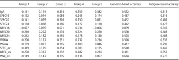
Correlations between PGEBV and adjusted phenotypes, with corresponding accuracies for each trait, for the cross-validation groups in the SBF population are reported in Table 1, together with the accuracies estimated using pedigree-based EBV. Correlations varied between groups, ranging from marginally negative (−0.027 in group 1 for Nematodirus FEC at 16 weeks) to positive and moderate (0.382 in group 5 for IgA). Moderate accuracies
 $$\left( {r_{{\hat{g}g}} } \right)$$
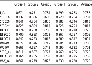
were observed, generally between 0.42 and 0.68, with the exception of the accuracy for Nematodirus FEC at 16 weeks (0.10), this being the trait with the lowest heritability. Accuracies using pedigree-based EBV ranged from 0.27 to 0.52, and were slightly lower than the genomic EBV accuracies for 9 of the 12 traits. The empirical standard error of the accuracy for Strongyles FEC average animal effect, estimated as the standard deviation of the accuracies across the 10 replicated cross-validations, was 0.04. Correlations between GEBV and PGEBV (Table 2), representing the relationship between genomic EBVs predicted with and without individual data, were all strong and positive. The average value across all traits was 0.76.
Correlations between predicted genomic estimated breeding values and adjusted phenotypes and accuraciesFootnote * for the random cross-validation groups both using the genomic relationship matrix and the pedigree-based relationship matrix in the Scottish Blackface population

IgA: Immunoglobulin-A; SFEC16, SFEC20 and SFEC24: faecal egg count at 16, 20 and 24 weeks for Strongyles, respectively; NFEC16, NFEC20 and NFEC24: faecal egg count at 16, 20 and 24 weeks for Nematodirus, respectively; W16W and W24W: BW at 16 and 24 weeks, respectively; SFEC_av, NFEC_av, WW_av: average animal effect for Strongyles and Nematodirus faecal egg count and for BW, respectively.
* Accuracy here is the average of the accuracies across validation sets, estimated as the correlation for each validation set divided by the square root of its heritability.
Correlations between genomic estimated breeding values and predicted estimated genomic breeding values for the random cross-validation groups in the Scottish Blackface population

IgA: Immunoglobulin-A; SFEC16, SFEC20 and SFEC24: faecal egg count at 16, 20 and 24 weeks for Strongyles, respectively; NFEC16, NFEC20 and NFEC24: faecal egg count at 16, 20 and 24 weeks for Nematodirus, respectively; W16W and W24W: BW at 16 and 24 weeks, respectively; SFEC_av, NFEC_av, WW_av: average animal effect for Strongyles and Nematodirus faecal egg count and for BW, respectively.
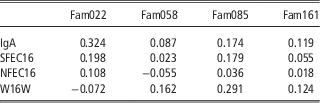
Lower correlation estimates between phenotype and PGEBV were obtained when all members in one sire family were predicted from the remaining sire families in the SBF data (Table 3). However, differences were observed in relationship connectivity between families. For example, nematode resistance indicator trait results (i.e. both IgA and FEC) showed that the families that were more closely related to the remaining families in the TS were those with more accurate PGEBV. In particular, the half-sib family sired by ram 22 (i.e. Fam22), which is the most highly related to the remaining TS families (data not shown), showed the highest correlations. However, different results were found for BW, suggesting that not only relatedness is important, but other factors (such as trait heritability or markers in LD with mutations affecting the trait) may play a part.
Correlations between predicted genomic estimated breeding values and adjusted phenotypes for families in the Scottish Blackface population

IgA: Immunoglobulin-A; SFEC16, NFEC16 and W16W: Strongyles and Nematodirus faecal egg count and BW at 16 weeks, respectively.
Across populations
The correlations between PGEBV and adjusted phenotype for the Strongyles average animal effect were −0.054, −0.030 and 0.005 for SBF v. (MBR plus SAR), MBR v. (SBF plus SAR) and SAR v. (SBF plus MBR) data sets, respectively. The correlations between PGEBV and adjusted phenotypes for the BT data v. SBF were −0.012, −0.010 and 0.067 for Strongyles and Nematodirus FEC at 20 weeks and for BW at 24 weeks, respectively. In both analyses, the predictions for genetically distant groups were usually close to zero. However, when 1 or 10 lambs from each sire family from the SBF data were randomly chosen and included in the TS, the correlations between PGEBV and y* were slightly higher, and always positive with 0.129 and 0.070 for SBF v. (MBR plus SAR plus 10SBF) and SBF v. (MBR plus SAR plus 100SBF), respectively.
Exploring contribution of population and genome structure
The results of the analysis in the SBF data, fitting either the A or G matrix alone, or both together, are reported in Supplementary Table S1. For some traits, the heritability estimates were either completely explained by the G matrix (i.e. IgA and Nematodirus FEC at 20 weeks) or the A matrix (Strongyles FEC at 20 weeks and Nematodirus FEC at 16 weeks) when the analysis was performed fitting both G and A matrices. However, for the other FEC traits (both Strongyles and Nematodirus), there was a contribution from both matrices. In general, there was little discernible pattern in these results. Moreover, the relative partitioning of genetic variation between the A and G matrices may be expected to vary as the number and size of families varies; thus, it is difficult to draw general conclusions from these results.
For the SBF population, heritability estimates were also obtained either fitting only one chromosome or when simultaneously fitting one chromosome plus the whole G matrix (results not shown). Although similar trends were observed, the proportions of genetic variation accounted for when fitting only one chromosome were always overestimated. However, in both cases, it is possible to identify the chromosomes that explain most of the genetic variation of the traits.
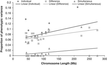
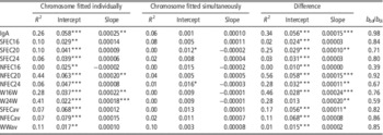
We tested the hypothesis that fitting all G ch (i.e. chromosome-wide genomic matrices) simultaneously would result in each chromosome explaining a fraction of the total genetic variance proportional to its length, consistent with the polygenic assumptions underlying genomic best linear unbiased predictors (GBLUP). Although there was a weak tendency for this to be the case for most traits (e.g. Figure 1), the majority of the captured genetic variation appeared to be independent of chromosome length. This can be seen in Table 4, which reports intercept, slope and R 2 for the three regressions (i.e. by fitting each chromosome individually, by fitting all chromosomes simultaneously, and the difference between the two), as well as the proportion of genetic variance explained by relatedness for all traits considered. These proportions (ranging from 0.39 to 0.98, with an average of 0.77) suggest that in most cases our accuracy estimates are mostly because of additive genetic relatedness, rather than LD between SNP and QTL. The A-matrix-derived heritabilities were compared with accuracies and proportion of genetic variance explained by relatedness (b 0d/b 0i) for all nematode resistance indicator traits (results not shown). Among the Strongyles FEC and IgA results, there was little discernible relationship between these variables. The Nematodirus traits were more variable; however, they tended to have lower heritabilities and relatively large genetic effects (i.e. QTL) that had previously been observed on some of the smaller chromosomes (see the ‘Discussion’ section), suggesting that the polygenic inheritance assumption was inappropriate for the Nematodirus traits.
Proportion of phenotypic variance explained per chromosome for Immunoglobulin-A (scattered points) and fitted regression (line). Chromosome fitted individually (top regression) or simultaneously (bottom regression). Middle regression results from plotting the difference between top and bottom regression.

Intercept, slope (i.e. proportion of phenotypic variance/Mb), and R 2 for the three regressions (i.e. by fitting each chromosome individually, by fitting all chromosomes simultaneously and the difference between the two) as well as the proportion of genetic variance explained by relatedness (b 0d/b 0i) for all traits considered

IgA: Immunoglobulin-A; SFEC16, SFEC20 and SFEC24: faecal egg count at 16, 20 and 24 weeks for Strongyles, respectively; NFEC16, NFEC20 and NFEC24: faecal egg count at 16, 20 and 24 weeks for Nematodirus, respectively; W16W and W24W: BW at 16 and 24 weeks, respectively; SFEC_av, NFEC_av, WW_av: average animal effect for Strongyles and Nematodirus faecal egg count and for BW, respectively.
*P<0.05; **P<0.01; ***P<0.001
Discussion
One of the objectives of the current study was to understand the dynamics of applying GS to hard-to-measure traits using field data. We assumed two scenarios, with the first scenario having young animals selected from markers before their phenotypes can be measured, and second, where we break the assumption that the animals of the TS and the validation sets are from the same population, that is, we explore situations where the animals vary from being closely related to unrelated. Therefore, we explored the possibility of using genomic predictions within and across populations; although prediction accuracies within a population were good, with a small empirical standard error, our results highlighted the difficulties of prediction using genetically distant individuals.
We also reported prediction accuracies estimated by using both the G and A relationship matrix. The accuracies estimated with the G matrix were usually higher that those with the A matrix, suggesting an advantage in using genomic information for predictions, even when pedigree knowledge is available. The one case where the accuracies estimated with the A matrix was substantially better, viz. Nematodirus FEC at 16 weeks, was for a trait for which heritability estimate was mostly explained by the A matrix (Supplementary Table S1).
Although several studies on GEBV accuracy/reliability estimated from real data have been reported in the literature for cattle with GEBV reliabilities ranging from 18% to 78% (Harris et al., Reference Harris, Johnson and Spelman2009; VanRaden et al., Reference VanRaden, Van Tassell, Wiggans, Sonstegard, Schnabel, Taylor and Schenkel2009; Hayes et al., Reference Hayes, Bowman, Chamberlain, Verbyla and Goddard2009b), fewer are reported for sheep. Our GEBV accuracies are similar to others obtained using a medium-density markers chip of 15% to 79% for wool traits in Merino sheep (Daetwyler et al., Reference Daetwyler, Hickey, Henshall, Dominik, Gredler, van der Werf and Hayes2010a), and 7% to 31% for carcass and meat-quality traits in multi-breed sheep data (Daetwyler et al., Reference Daetwyler, Swan, van der Werf and Hayes2012b). In a study on the Lacaune dairy sheep breed using different genomic methods, Duchemin et al. (Reference Duchemin, Colombani, Legarra, Baloche, Larroque, Astruc, Barillet, Robert-Granié and Manfredi2012) reported accuracies varying from 0.4 to 0.6, according to the traits (i.e. milk yield, fat content and somatic cell scores), with minor differences among genomic approaches. These authors also showed that the inclusion of molecular information, as compared with traditional schemes, increased accuracies of EBV of young males at birth from 18% up to 25%, according to the trait (Duchemin et al., Reference Duchemin, Colombani, Legarra, Baloche, Larroque, Astruc, Barillet, Robert-Granié and Manfredi2012). However, it has to be considered that the accuracy of the GEBV depends on the size of the population and on the heritability of the trait. For low heritability traits, a very large number of records will be required in the TS to subsequently achieve high accuracies of GEBV in unphenotyped animals. If we consider our SBF population, where the effective population size (Ne) is ~500 (Kijas et al., Reference Kijas, Lenstra, Hayes, Boitard, Porto Neto, San Cristobal, Servin, McCulloch, Whan, Gietzen, Paiva, Barendse, Ciani, Raadsma, McEwan and Dalrymple2012), then according to the formula suggested by Daetwyler et al. (Reference Daetwyler, Pong-Wong, Villanueva and Woolliams2010b) to achieve an accuracy of 0.6, we would need ~30 000 individuals for a trait with very low heritability (e.g. Nematodirus FEC at 16 weeks), and ~5000 for a trait with moderate heritability (e.g. IgA).
The current study explored the contributions of LD and relatedness to the accuracies of genomic predictions. The heritability estimates obtained either fitting only one chromosome or when simultaneously fitting one chromosome plus the whole G matrix showed that nematode resistance in sheep is a complex trait with contributions from many regions in the genome affecting these traits. However, with the exception of Nematodirus FEC at 16 weeks (Supplementary Figure S2; Riggio et al., Reference Riggio, Matika, Pong-Wong, Stear and Bishop2013), the results favour a polygenic mode of inheritance, which is largely captured by additive relationships between animals. This is illustrated by the results when a chromosome at a time was fitted that overestimated the proportion of genetic variance explained as opposed to when one chromosome and the G matrix were simultaneously fitted. As highlighted by Daetwyler et al. (Reference Daetwyler, Kemper, van der Werf and Hayes2012a), if the only contribution of the SNPs to the accuracy of genomic prediction was through LD with QTL, and assuming a polygenic model, then a G matrix constructed from only the SNPs on one chromosome should capture genetic variation in proportion to its length, assuming that there is no population stratification. However, this was not the case in our study. It was therefore clear that a large proportion of the accuracy of genomic prediction in the SBF population, at the current SNP density, is because of population structure, that is, relatedness between animals. In other words, only a small proportion of the accuracy was because of LD between SNP and QTL.
This proposition was tested formally using the regression approach suggested by Yang et al. (Reference Yang, Manolio, Pasquale, Boerwinkle, Caporaso, Cunningham, de Andrade, Feenstra, Feingold, Hayes, Hill, Landi, Alonso, Lettre, Lin, Ling, Lowe, Mathias, Melbye, Pugh, Cornelis, Weir, Goddard and Visscher2011). The intercept (b 0d) of the difference between the variance for each chromosome when analysed individually or simultaneously was highly significant for all traits (P<0.0001), with the exception of BW at 24 weeks (P=0.09). On the other hand, the slope (b 1d ) of the difference was significant only for some of the traits. These values show the importance of the relatedness in our SBF population, suggesting that most of our accuracy is probably captured by additive relatedness. The ratio b 0d/b 0i is a measure of the proportion of genetic variance explained by such relatedness (Yang et al., Reference Yang, Manolio, Pasquale, Boerwinkle, Caporaso, Cunningham, de Andrade, Feenstra, Feingold, Hayes, Hill, Landi, Alonso, Lettre, Lin, Ling, Lowe, Mathias, Melbye, Pugh, Cornelis, Weir, Goddard and Visscher2011), and with the exception of NFEC16, this measure was high (0.59 to 0.98) and therefore accounted for most of the variation in our SBF GEBV predictions. Of interest is the observation that accuracy and the component because of relatedness were largely independent of the A-matrix-derived heritability estimates (results not shown).
The impact of relatedness has been previously studied, and differences in accuracies have been ascribed to the number of relatives in the TS and the degree of additive–genetic relationships with training individuals (Habier et al., Reference Habier, Tetens, Seefried, Lichtner and Thaller2010). Legarra et al. (Reference Legarra, Robert-Granie, Manfredi and Elsen2008) analysed accuracies of GEBV for individuals either related or unrelated to the TS in a mouse population, concluding that markers were able to recover family information to some extent. Our choice of predicting all members of a single sire family from the remaining sire families in the SBF data was designed to reduce the upward biases of accuracies resulting from within-family prediction when half-sib families are randomly split between TS and validation sets. In this case, we showed that the closer the individuals in the validation set are to the TS, the higher the accuracy. This is probably partly owing to the fact that genomic predictions across closely related individuals capture linkage effects, whereas those across distantly related animals require LD between SNP and QTL. However, it should be noted that, although we used distinct sire families with the SBF data, these families were in most part also closely related.
We also estimated the accuracy achieved when predicting breeding values across populations. These across-population accuracies were very low, sometimes even negative. These low estimates may be explained by extension from our previous results. First, much of the accuracy in the SBF data set was because of additive genetic relationships between animals, as captured by the marker–IBS relationships. This will not be possible in distant populations. Second, the component of accuracy because of LD between SNP and QTL is also likely to be low in distant breeds, as the linkage phase between SNP and QTL will differ randomly in different breeds. The more distant the relationship between individuals, the shorter the genomic distance over which phase will be consistent. This outcome is reinforced by the finding that the accuracy achieved for across-population prediction was somewhat higher when a small number of animals from the population to be predicted were included in the TS.
It has been suggested that the use of a different method (i.e. BayesSSVS; Verbyla et al., Reference Verbyla, Hayes, Bowman and Goddard2009) could increase across-breed prediction, as it assigns SNPs to either a distribution with very small variance (i.e. near 0) or one with a larger variance in the prediction model, unlike GBLUP that assumes that all SNP effects are sampled from distributions with the same variance (Daetwyler et al., Reference Daetwyler, Kemper, van der Werf and Hayes2012a). However, this suggestion presupposes that the same gene variants are segregating in different populations, and that the SNP density is sufficient for there to be consistent LD between marker and QTL in (some of) the different populations. It has been suggested that the number of SNPs needed to predict unrelated individuals is equal to 10 NeL, where L is the length of the genome in Morgans (Meuwissen, Reference Meuwissen2009). In the SBF population, with Ne of ~500 (Kijas et al., Reference Kijas, Lenstra, Hayes, Boitard, Porto Neto, San Cristobal, Servin, McCulloch, Whan, Gietzen, Paiva, Barendse, Ciani, Raadsma, McEwan and Dalrymple2012) and L of approximately 27 Morgans, predictions for unrelated individuals would require at least 135 000 SNPs. This marker density may be achievable with the forthcoming high-density sheep SNP chip.
In summary, we have applied genomic prediction techniques to nematode resistance and BW data and found GEBV, which, at first sight, appeared to have moderate to good within-population predictive accuracy, despite a relatively limited TS. However, much of the accuracy achieved appears to be a result of the markers capturing additive genetic relationships between animals in the population. This is reinforced by the observations that (i) the accuracy tends to drop when predictions are across more distantly related animals in the same population, (ii) across-population predictions have accuracies close to zero and (iii) some across-population accuracy can be recovered by including a small number of animals from the target population in the TS. These results suggest that genomic prediction for nematode resistance and BW may be of value in closely related animals, but with the current SNP chip genomic predictions are unlikely to work across breeds.
Acknowledgements
These results are obtained through the EC-funded FP7 Project 3SR-245140. French SNP data were funded by the SHEEPSNPQTL ANR project. Funding from the Regional Government of Sardinia contributed to the collection of Sardinian SNP and phenotype data. We also wish to acknowledge funding contributions from EADGENE_S, the BBSRC Institute Strategic Programme Grant at The Roslin Institute and the Scottish Government’s Strategic Partnership for Animal Science Excellence (SPASE) initiative.