1 A new two-fluid wave labelling scheme
Any fluid theory, such as the single-fluid magnetohydrodynamic (MHD) (e.g. Goedbloed & Poedts Reference Goedbloed and Poedts2004; Goedbloed, Keppens & Poedts Reference Goedbloed, Keppens and Poedts2010, Reference Goedbloed, Keppens and Poedts2019) or its two-fluid (electron–ion) extension, is based on taking moments of the kinetic equations, where a closure relation is needed. For example, the cold two-fluid theory (electron–ion) only involves zeroth- and first-order moments, neglecting finite pressure effects, while the warm two-fluid theory brings in the second moment through the plasma species pressures. As detailed in chapter 3 of Goedbloed et al. (Reference Goedbloed, Keppens and Poedts2019), many assumptions enter in this truncation procedure, involving all intricacies of classical transport theory. An interesting observation, pointed out in the same textbook, is how a maximal ordering argument of the involved plasma length scales directly leads from the two-fluid prescription to the MHD one, without relying on the smallness of the ratio
 $\unicode[STIX]{x1D707}=Zm_{e}/m_{p}$
of masses over charges (electron mass
 $m_{e}$
and ion mass
 $m_{p}$
, with charge number
 $Z$
). In particular, the MHD limit is thus perfectly adequate for a pair plasma where
 $\unicode[STIX]{x1D707}=1$
, when restricting attention to large scale phenomena, accounting for all effects of inhomogeneities in physical space (but missing out effects of inhomogeneities in velocity space). We therefore expect to retrieve exact MHD limits for wave dynamics in two-fluid plasmas, and this point motivated our study of all waves present in cold and warm two-fluid pair plasmas.
Although the ideal two-fluid viewpoint on a plasma fails to describe a number of important effects related to wave propagation, with wave–particle interaction à la Landau as its most serious omission, it clearly shows how the usual one-fluid MHD picture of plasma dynamics is enriched by electrostatic and electromagnetic (i.e. light) wave signals. In two recent works (Keppens & Goedbloed Reference Keppens and Goedbloed2019a
,Reference Keppens and Goedbloed
b
), we revisited this established theory on wave propagation in uniform plasma conditions, which always looks at plane wave solutions, such that a Fourier description can adopt
 $\exp [\text{i}(\boldsymbol{k}\boldsymbol{\cdot }\boldsymbol{x}-\unicode[STIX]{x1D714}t)]$
, introducing the wavevector
 $\boldsymbol{k}$
and frequency
 $\unicode[STIX]{x1D714}$
. In both works, we demonstrated the advantages of using the governing 12th degree polynomial in the wave frequency
 $\unicode[STIX]{x1D714}$
, which can be derived from linearizing the governing two-fluid and Maxwell equations (Denisse & Delcroix Reference Denisse and Delcroix1961). That there indeed are twelve non-trivial waves, which separate into six pairs of forward–backward propagating waves, as the polynomial is sixth order in
 $\unicode[STIX]{x1D714}^{2}$
, is pointed out in several textbooks (e.g. Goedbloed & Poedts Reference Goedbloed and Poedts2004; Kulsrud Reference Kulsrud2005; Goedbloed et al.
Reference Goedbloed, Keppens and Poedts2019). Since many classical textbooks (e.g. Stix Reference Stix1992; Boyd & Sanderson Reference Boyd and Sanderson2003; Bittencourt Reference Bittencourt2004; Gurnett & Bhattacharjee Reference Gurnett and Bhattacharjee2005; Kulsrud Reference Kulsrud2005; Chen Reference Chen2016; Thorne & Blandford Reference Thorne and Blandford2017) start with presenting the special case of a cold plasma, where only five non-trivial pairs remain, our earlier works (Keppens & Goedbloed Reference Keppens and Goedbloed2019a
,Reference Keppens and Goedbloed
b
) focused on these five, and suggested a convenient labelling that relates to their ordered appearance at long wavelengths. Indeed, the cold case contains two modes that become the low frequency, long wavelength MHD Alfvén (A) and fast (F) magnetosonic modes. Together with the modified electrostatic (M) plasma oscillation (i.e. modified when going from unmagnetized, where it does not propagate, to propagating in magnetized cases) and the two electromagnetic O and X wave modes, the suggested A, F, M, O and X labels were shown to be unambiguous in identifying waves for both cold pair (Keppens & Goedbloed Reference Keppens and Goedbloed2019b
) and cold ion–electron plasmas (Keppens & Goedbloed Reference Keppens and Goedbloed2019a
). In particular, their use improves on the fact that:
(i) the usual means of working with left and right (L/R) labels does not apply in pair plasmas (Keppens & Goedbloed Reference Keppens and Goedbloed2019b ) and was found to mix forward and backward waves between the five remaining wave pairs (Keppens & Goedbloed Reference Keppens and Goedbloed2019a );
(ii) cold plasmas are known to have branches that can cross only at purely parallel or purely perpendicular orientations (Gurnett & Bhattacharjee Reference Gurnett and Bhattacharjee2005) and these orientations are therefore best treated as special cases. We return to this issue in the present manuscript: avoided crossings can be identified precisely;
(iii) the established distinction between ordinary (O) and extraordinary waves is yet another example where multiple solutions get mixed up, since the extraordinary branch (E or X, depending on the textbook at hand) really accounts for three wave modes;
(iv) the use of fast–slow (F/S) labels for characterizing the maximal number of two propagating wave modes in a cold plasma at a fixed frequency is rather confusing and shown to be in conflict with the established naming convention of slow, Alfvén and fast waves in MHD theory (Keppens & Goedbloed Reference Keppens and Goedbloed2019a ). Moreover, in a warm plasma, up to four different wave modes can occur at a fixed frequency, so the traditional F/S labels from cold plasma theory become meaningless. We will therefore use the F and S label differently, namely in direct correspondence with the MHD fast and slow magnetosonic waves.
In this paper, we will hence study the more general case of a warm plasma, but restrict our attention to pair plasmas. In that case, the general dispersion relation also covers the slow MHD waves (S), and the unique labelling scheme for waves in a warm pair plasma will thus logically consist of S, A, F, M, O and X wave modes.
2 Motivation
The study of waves in pair plasmas is of great interest to both laboratory and astrophysical contexts: recent breakthroughs in generating laboratory pair plasmas will lead to fundamental insight into their behaviour (Sarri et al. Reference Sarri, Poder, Cole, Schumaker, di Piazza, Reville, Dzelzainis, Doria, Gizzi and Grittani2015), while pair plasmas are believed to be especially relevant for pulsar magnetosphere processes (Lyutikov Reference Lyutikov1999). The fact that a pair plasma has a unit mass ratio between its constituent species (electrons and positrons) makes it more amenable to detailed numerical studies by means of particle-in-cell treatments (Bret & Narayan Reference Bret and Narayan2018; Loureiro & Boldyrev Reference Loureiro and Boldyrev2018; Zenitani Reference Zenitani2018), which do account for the kinetic physics missing in the two-fluid approach. At the same time, this mass symmetry between the negative and positive charge species significantly complicates its theoretical treatment: in normal ion–electron plasmas, the mass ratio between electrons and ions serves as a small parameter and introduces a convenient split between high (electrostatic and electromagnetic) and low (MHD like) frequency wave modes. Throughout the plasma literature, numerous examples exist which then focus on either of these two families, each consisting of three (or sometimes up to four) mode types (Stringer Reference Stringer1963; Ishida, Cheng & Peng Reference Ishida, Cheng and Peng2005; Damiano, Wright & McKenzie Reference Damiano, Wright and McKenzie2009; Bellan Reference Bellan2012; Zhao Reference Zhao2015, Reference Zhao2017). For example, the frequently exploited Appleton–Hartree dispersion relation was shown to be such a mass-ratio-based reduction (Keppens & Goedbloed Reference Keppens and Goedbloed2019a ), where the remaining four high frequency mode types are known as the whistler wave (our F mode), the so-called Z mode (our M wave) and the free space electromagnetic L-O (i.e. our O) and R-X (i.e. our X) modes (Gurnett & Bhattacharjee Reference Gurnett and Bhattacharjee2005). In the same paper (Keppens & Goedbloed Reference Keppens and Goedbloed2019a ), we also identified a serious shortcoming of the Appleton–Hartree description: it simply does not capture the proper wave behaviour at high (up to relativistic) magnetizations. The present warm pair plasma analysis will be fully applicable to the relativistic regime, similar to our cold plasma treatment.
The two-fluid approach will exploit normalized quantities in what follows, where we scale all frequencies to the combined electron–positron plasma frequency, i.e.
 $\unicode[STIX]{x1D714}\equiv \unicode[STIX]{x1D714}/\unicode[STIX]{x1D714}_{p}$
, where
 $\unicode[STIX]{x1D714}_{p}^{2}=\unicode[STIX]{x1D714}_{pe}^{2}+\unicode[STIX]{x1D714}_{pp}^{2}$
, where the electron and positron plasma frequencies are equal and both given by
 $\unicode[STIX]{x1D714}_{pe}=\sqrt{e^{2}n_{e}/\unicode[STIX]{x1D716}_{0}m_{e}}$
as their number densities are equal
 $n_{e}=n_{p}$
, as well as their masses
 $m_{e}=m_{p}$
. The speed of light
 $c$
obeys
 $c^{2}=1/\unicode[STIX]{x1D707}_{0}\unicode[STIX]{x1D716}_{0}$
, and is used to define the skin depth
 $\unicode[STIX]{x1D6FF}=c/\unicode[STIX]{x1D714}_{p}$
, which then allows us to work with normalized wavenumbers
 $k\equiv \unicode[STIX]{x1D6FF}k$
. This is adopted throughout the manuscript.
3 Symmetrized governing equations
Our starting point is the following, completely symmetric form of the linearized ideal two-fluid equations (Goedbloed & Poedts Reference Goedbloed and Poedts2004; Goedbloed et al. Reference Goedbloed, Keppens and Poedts2019), for the particular case of a warm pair plasma:
 $$\begin{eqnarray}\displaystyle \!\!\left(\begin{array}{@{}cccccc@{}}\unicode[STIX]{x1D714}^{2}-k^{2} & 0 & \unicode[STIX]{x1D714}/\sqrt{2} & 0 & -\unicode[STIX]{x1D714}/\sqrt{2} & 0\\ 0 & \unicode[STIX]{x1D714}^{2}-k^{2}-1 & \unicode[STIX]{x1D706}E/\sqrt{2} & \unicode[STIX]{x1D70F}E/\sqrt{2} & \unicode[STIX]{x1D706}E/\sqrt{2} & \unicode[STIX]{x1D70F}E/\sqrt{2}\\ \unicode[STIX]{x1D714}/\sqrt{2} & \unicode[STIX]{x1D706}E/\sqrt{2} & \unicode[STIX]{x1D714}^{2}-\unicode[STIX]{x1D706}^{2}E^{2} & -\unicode[STIX]{x1D706}\unicode[STIX]{x1D70F}E^{2} & 0 & 0\\ 0 & \unicode[STIX]{x1D70F}E/\sqrt{2} & -\unicode[STIX]{x1D706}\unicode[STIX]{x1D70F}E^{2} & \begin{array}{@{}c@{}}\unicode[STIX]{x1D714}^{2}-k^{2}v^{2}\\ -\frac{1}{2}-\unicode[STIX]{x1D70F}^{2}E^{2}\end{array} & 0 & \frac{1}{2}\\ -\unicode[STIX]{x1D714}/\sqrt{2} & \unicode[STIX]{x1D706}E/\sqrt{2} & 0 & 0 & \unicode[STIX]{x1D714}^{2}-\unicode[STIX]{x1D706}^{2}E^{2} & -\unicode[STIX]{x1D706}\unicode[STIX]{x1D70F}E^{2}\\ 0 & \unicode[STIX]{x1D70F}E/\sqrt{2} & 0 & \frac{1}{2} & -\unicode[STIX]{x1D706}\unicode[STIX]{x1D70F}E^{2} & \begin{array}{@{}c@{}}\unicode[STIX]{x1D714}^{2}-k^{2}v^{2}\\ -\frac{1}{2}-\unicode[STIX]{x1D70F}^{2}E^{2}\end{array}\end{array}\right)\!\left(\begin{array}{@{}c@{}}\tilde{E}_{1}\\ \tilde{E}_{2}\\ \tilde{U} _{e1}\\ \tilde{U} _{e3}\\ \tilde{U} _{p1}\\ \tilde{U} _{p3}\end{array}\right)\!=0.\hspace{-10.79993pt} & & \displaystyle \nonumber\\ \displaystyle & & \displaystyle\end{eqnarray}$$
In this equation, we used the following notation
 $$\begin{eqnarray}\displaystyle & \unicode[STIX]{x1D70F}=\sin \unicode[STIX]{x1D717}, & \displaystyle\end{eqnarray}$$
 $$\begin{eqnarray}\displaystyle & \unicode[STIX]{x1D706}=\cos \unicode[STIX]{x1D717}, & \displaystyle\end{eqnarray}$$
where
 $\unicode[STIX]{x1D717}$
denotes the angle between the wavevector
 $\boldsymbol{k}$
and the magnetic field vector
 $\boldsymbol{B}$
. The latter two vectors were used to introduce properly scaled components of the linear electric field perturbation
 $\tilde{\boldsymbol{E}}$
and electron and positron flow perturbations
 $\tilde{\boldsymbol{u}}_{e,p}$
, as follows:
 $$\begin{eqnarray}\left.\begin{array}{@{}c@{}}\hat{\boldsymbol{e}}_{1}=\hat{\boldsymbol{e}}_{2}\times \hat{\boldsymbol{e}}_{3},\\ \hat{\boldsymbol{e}}_{2}=\boldsymbol{B}\times \boldsymbol{k}/|\boldsymbol{B}\times \boldsymbol{k}|,\\ \hat{\boldsymbol{e}}_{3}=\boldsymbol{k}/|\boldsymbol{k}|,\end{array}\right\}\quad \left.\begin{array}{@{}c@{}}\tilde{E}_{1}=\text{i}\sqrt{\unicode[STIX]{x1D716}_{0}}\,\tilde{\boldsymbol{E}}\boldsymbol{\cdot }\hat{\boldsymbol{e}}_{1},\\ \tilde{E}_{2}=\sqrt{\unicode[STIX]{x1D716}_{0}}\,\tilde{\boldsymbol{E}}\boldsymbol{\cdot }\hat{\boldsymbol{e}}_{2},\\ \tilde{U} _{e\,1,3}=\sqrt{n_{e}m_{e}}\,\tilde{\boldsymbol{u}}_{e}\boldsymbol{\cdot }\hat{\boldsymbol{e}}_{1,3},\\ \tilde{U} _{p\,1,3}=\sqrt{n_{p}m_{p}}\,\tilde{\boldsymbol{u}}_{p}\boldsymbol{\cdot }\hat{\boldsymbol{e}}_{1,3}.\end{array}\right\}\end{eqnarray}$$
This particular scaling and choice for the linearized variables ensures that we obtain a symmetric
 $6\times 6$
matrix in (3.1). Note that
 $\hat{\boldsymbol{e}}_{2}$
is ill defined for parallel propagation
 $\boldsymbol{k}\Vert \boldsymbol{B}$
, as there is freedom to then choose any set of orthogonal basis vectors in the plane perpendicular to
 $\boldsymbol{k}$
. The dispersion relation, obtained from the vanishing determinant of this real symmetric matrix, becomes a simple twelfth-order polynomial in
 $\unicode[STIX]{x1D714}$
, which is sixth order in
 $\unicode[STIX]{x1D714}^{2}$
. Note that only two parameters
 $(E^{2},v^{2})$
appear in (3.1), once a particular choice for the orientation
 $\unicode[STIX]{x1D717}$
is made: these are in the original derivation presented in Goedbloed & Poedts (Reference Goedbloed and Poedts2004) given by
 $$\begin{eqnarray}\displaystyle & \displaystyle E^{2}=\frac{B^{2}}{\unicode[STIX]{x1D707}_{0}\unicode[STIX]{x1D70C}c^{2}}, & \displaystyle\end{eqnarray}$$
 $$\begin{eqnarray}\displaystyle & \displaystyle v^{2}=\frac{\unicode[STIX]{x1D6FE}p}{\unicode[STIX]{x1D70C}c^{2}}, & \displaystyle\end{eqnarray}$$
where we used the combined pressure
 $p=p_{e}+p_{p}=2p_{e}$
and combined density
 $\unicode[STIX]{x1D70C}=n_{e}m_{e}+n_{p}m_{p}=2n_{e}m_{e}$
, with equal electron and positron number densities
 $n_{e}=n_{p}$
for charge neutrality. This uses a fiducial polytropic index
 $\unicode[STIX]{x1D6FE}$
, and adopts equal temperatures for the electron–positron plasma constituents.
The six linear equations retained in (3.1) conveniently reduced the original set of 18 equations, which linearized the five (mass, momentum and energy) conservation laws per species, augmented with the eight Maxwell equations. In terms of linear wave modes
 $\unicode[STIX]{x1D714}$
, the original set counts 14 modes, since the time-independent Maxwell equations act as constraints. Two marginal modes (i.e. a pair
 $\unicode[STIX]{x1D714}^{2}=0$
) were further eliminated, which represent the entropy modes familiar from linear MHD theory. Only the inclusion of non-adiabatic effects makes those modes relevant for further analysis (Claes & Keppens Reference Claes and Keppens2019). The remaining six mode pairs in the dispersion relation obtained from (3.1) will occupy us in what follows.
As a final note on the
 $6\times 6$
matrix formulation from (3.1), its real and symmetric nature implies that this matrix has always a set of six real matrix eigenvalues
 $(\unicode[STIX]{x1D706}_{1},\ldots ,\unicode[STIX]{x1D706}_{6})$
, for which we will always be able to find a set of six orthonormal eigenvectors. The wave modes following from the dispersion relation
 $\unicode[STIX]{x1D714}(k)=0$
make at least one of these matrix eigenvalues zero. When the zero matrix eigenvalue has an algebraic multiplicity of two, there is some freedom in choosing the set of two orthonormal eigenvectors within the then two-dimensional eigenspace of this zero eigenvalue. This occurs when two of the
 $\unicode[STIX]{x1D714}(k)$
branches cross, and we will pay specific attention to these crossings. The discussion of actual polarization properties related to the six wave pairs best starts from the real and symmetric matrix above, using its eigenvectors. This is illustrated in appendix A.
4 Dispersion relation and relativistic validity
The dispersion relation
 $\unicode[STIX]{x1D714}(k)=0$
for the six non-trivial mode pairs follows from setting the determinant of the matrix in (3.1) to zero. This gives a sixth-order polynomial in
 $\unicode[STIX]{x1D714}^{2}$
, with coefficients depending on
 $E^{2}$
,
 $v^{2}$
,
 $\unicode[STIX]{x1D706}^{2}$
and
 $k^{2}$
. At a fixed frequency
 $\unicode[STIX]{x1D714}$
and for a set of
 $(E^{2},v^{2},\unicode[STIX]{x1D706}^{2})$
, we get a fourth-order polynomial in
 $k^{2}$
. In the cold case
 $v^{2}=0$
, the same dispersion relation becomes only second order in
 $k^{2}$
, and this inspired all textbook theory to use these maximal two propagating waves at fixed frequency and refer to them as ‘fast’ and ‘slow’, and to produce e.g. the familiar Clemmow–Mullaly–Allis or CMA diagrams (Clemmow & Mullaly Reference Clemmow and Mullaly1955; Stix Reference Stix1992; Gurnett & Bhattacharjee Reference Gurnett and Bhattacharjee2005; Thorne & Blandford Reference Thorne and Blandford2017). We will use both polynomial viewpoints (i.e., in either
 $k^{2}$
or
 $\unicode[STIX]{x1D714}^{2}$
) in our discussion that follows. In Keppens & Goedbloed (Reference Keppens and Goedbloed2019a
) we discussed the disadvantages of using the CMA means to visualize wave properties for a cold ion–electron plasma. Instead, five-mode phase and group diagrams were introduced, which in the present warm pair case will become six-mode phase and group diagrams.
4.1 Factorizing the dispersion relation
The dispersion relation for warm pair plasmas turns out to factorize into two separate branches. These are given by
 $$\begin{eqnarray}\displaystyle \text{X},\text{F},\text{S}: & & \displaystyle \unicode[STIX]{x1D714}^{6}-\unicode[STIX]{x1D714}^{4}(1+k^{2}+E^{2}+v^{2}k^{2})+\unicode[STIX]{x1D714}^{2}k^{2}(E^{2}+v^{2}+v^{2}E^{2}\unicode[STIX]{x1D706}^{2}+v^{2}k^{2})\nonumber\\ \displaystyle & & \displaystyle \quad -\,E^{2}v^{2}k^{4}\unicode[STIX]{x1D706}^{2}=0,\end{eqnarray}$$
and
 $$\begin{eqnarray}\displaystyle \text{O},\text{M},\text{A}: & & \displaystyle \unicode[STIX]{x1D714}^{6}-\unicode[STIX]{x1D714}^{4}(2+k^{2}+E^{2}+v^{2}k^{2})\nonumber\\ \displaystyle & & \displaystyle \quad +\,\unicode[STIX]{x1D714}^{2}[1+E^{2}+k^{2}(1+E^{2}+v^{2}+v^{2}E^{2}\unicode[STIX]{x1D706}^{2}+v^{2}k^{2})]\nonumber\\ \displaystyle & & \displaystyle \quad -\,E^{2}k^{2}\unicode[STIX]{x1D706}^{2}-E^{2}v^{2}k^{4}\unicode[STIX]{x1D706}^{2}=0.\end{eqnarray}$$
The labels in front of the equations already introduce the six wave mode pairs we will find, and they contain the Alfvén (A) and fast (F) related modes, also present in the cold (pair or ion–electron) plasma case (Keppens & Goedbloed Reference Keppens and Goedbloed2019a
,Reference Keppens and Goedbloed
b
), along with the modified electrostatic (M) and electromagnetic O and X branches. The sixth mode pair, which was marginal for the cold case, is labelled S for slow magnetosonic. One can verify that the
 $v^{2}=0$
limit reduces to the cold pair case discussed in Keppens & Goedbloed (Reference Keppens and Goedbloed2019b
), where the X and F branches become angle independent:
 $v^{2}=0$
makes
 $\unicode[STIX]{x1D706}^{2}$
disappear from (4.1). This meant that both X and F branches behaved isotropically in a cold pair plasma, but this isotropy is gone for warm pair plasmas.
The fact that we can split the six mode pairs for a pair plasma into two branches was already noted by Stewart & Laing (Reference Stewart and Laing1992), who rather exploited the dielectric tensor means for obtaining the dispersion relation. In terms of polarization, the X, F, S branch has its electric field perturbation purely perpendicular to
 $\boldsymbol{k}$
and
 $\boldsymbol{B}$
(hence
 $\tilde{E}_{1}=0=\tilde{E}_{3}$
, with only
 $\tilde{E}_{2}\neq 0$
), while the O, M, A branch has a more involved variation in its orientation of
 $\tilde{\boldsymbol{E}}$
with respect to
 $\boldsymbol{k}$
and
 $\boldsymbol{B}$
, but has
 $\tilde{E}_{2}=0$
. As noted above, a full quantification of the polarization properties should employ the eigenvectors of the real and symmetric
 $6\times 6$
matrix, as illustrated in appendix A.
The two separate branches in the warm pair case are completely independent of each other, and no mode conversions between them can ever occur. Within a sub-branch of three modes, either X, F and S, or O, M and A, conversions do occur, as discussed further on. Note that this makes it impossible to find a split in the wave modes in high and low frequency branches, as is commonly adopted for ion–electron plasmas such as a fully ionized hydrogen plasma. In that case, the mass ratio between ions and electrons allows us to get approximate relations for the high frequency (these would be X, O and M) modes or for the low frequency MHD modes (S, A, F) separately. For example, this leads to the Appleton–Hartree dispersion relation for a cold ion–electron plasma (Keppens & Goedbloed Reference Keppens and Goedbloed2019a ), but this Appleton–Hartree dispersion relation is simply not applicable to the (cold or warm) pair plasma case.
4.2 Relativistic validity
Our starting equations presented in § 3 used the full Maxwell equations, and Newtonian versions of the rest frame linearized conservation laws (mass, momentum, energy). This, for example, led to the expressions (3.5)–(3.6) for the parameters
 $E^{2}$
and
 $v^{2}$
, where also a polytropic index
 $\unicode[STIX]{x1D6FE}$
appears. However, we will argue that a full relativistic treatment should lead to the same dispersion relation, where
 $E^{2}$
and
 $v^{2}$
then become the magnetization and the squared sound speed, respectively. Indeed, it is possible to rearrange the expressions (4.1)–(4.2) and write them in terms of the refractive index
 $n^{2}=k^{2}/\unicode[STIX]{x1D714}^{2}$
. This yields simply
 $$\begin{eqnarray}\displaystyle \text{X},\text{F},\text{S}: & & \displaystyle n^{4}v^{2}(\unicode[STIX]{x1D714}^{2}-E^{2}\unicode[STIX]{x1D706}^{2})+n^{2}[E^{2}+v^{2}(1+E^{2}\unicode[STIX]{x1D706}^{2})-\unicode[STIX]{x1D714}^{2}(1+v^{2})]\nonumber\\ \displaystyle & & \displaystyle \quad +\,\unicode[STIX]{x1D714}^{2}-1-E^{2}=0,\end{eqnarray}$$
and
 $$\begin{eqnarray}\displaystyle \text{O},\text{M},\text{A}: & & \displaystyle n^{2}[k^{2}v^{2}(\unicode[STIX]{x1D714}^{2}-E^{2}\unicode[STIX]{x1D706}^{2})-\unicode[STIX]{x1D714}^{4}(1+v^{2})+\unicode[STIX]{x1D714}^{2}(1+E^{2}+v^{2}+v^{2}E^{2}\unicode[STIX]{x1D706}^{2})-E^{2}\unicode[STIX]{x1D706}^{2}]\nonumber\\ \displaystyle & & \displaystyle \quad +\,\unicode[STIX]{x1D714}^{4}-\unicode[STIX]{x1D714}^{2}(2+E^{2})+1+E^{2}=0.\end{eqnarray}$$
We then read off the low frequency, long wavelength limits, where we expect to retrieve the finite
 $n^{2}$
expressions for the slow, Alfvén and fast magnetosonic modes. We find
 $$\begin{eqnarray}\displaystyle & E^{2}v^{2}\unicode[STIX]{x1D706}^{2}n^{4}-[E^{2}+v^{2}(1+E^{2}\unicode[STIX]{x1D706}^{2})]n^{2}+1+E^{2}=0, & \displaystyle\end{eqnarray}$$
 $$\begin{eqnarray}\displaystyle & -E^{2}\unicode[STIX]{x1D706}^{2}n^{2}+1+E^{2}=0. & \displaystyle\end{eqnarray}$$
These are the correct ideal relativistic MHD expressions for the slow, fast and Alfvén speeds, usually written as
 $$\begin{eqnarray}\left.\begin{array}{@{}c@{}}\displaystyle \unicode[STIX]{x1D714}_{S,F}^{2}=\frac{k^{2}}{2}\left[\frac{E^{2}+v^{2}(1+E^{2}\unicode[STIX]{x1D706}^{2})}{1+E^{2}}\pm \sqrt{\left(\frac{E^{2}+v^{2}(1+E^{2}\unicode[STIX]{x1D706}^{2})}{1+E^{2}}\right)^{2}-\frac{4\unicode[STIX]{x1D706}^{2}E^{2}v^{2}}{1+E^{2}}}\right],\\ \displaystyle \unicode[STIX]{x1D714}_{A}^{2}=\frac{k^{2}\unicode[STIX]{x1D706}^{2}E^{2}}{1+E^{2}}.\end{array}\right\}\end{eqnarray}$$
The point to note is that these ideal MHD expressions exploit the following, relativistically correct, magnetization and sound speed:
 $$\begin{eqnarray}\displaystyle & \displaystyle E^{2}=\frac{B^{2}}{\unicode[STIX]{x1D707}_{0}\unicode[STIX]{x1D70C}h}, & \displaystyle\end{eqnarray}$$
 $$\begin{eqnarray}\displaystyle & \displaystyle v^{2}=\frac{c_{g}^{2}}{c^{2}}, & \displaystyle\end{eqnarray}$$
where
 $h=c^{2}+\unicode[STIX]{x1D716}+p/\unicode[STIX]{x1D70C}$
is the specific enthalpy, using the rest frame specific internal energy
 $\unicode[STIX]{x1D716}$
. We note that the magnetization parameter
 $E^{2}$
is frequently written as
 $\unicode[STIX]{x1D70E}$
in single-fluid MHD theory (see also Keppens & Goedbloed Reference Keppens and Goedbloed2019a
), but for consistency with our previous works, we retain the symbol
 $E^{2}$
here. For a polytropic equation of state where
 $\unicode[STIX]{x1D70C}\unicode[STIX]{x1D716}=p/(\unicode[STIX]{x1D6FE}-1)$
, this leads to the expression for the sound speed as
 $c_{g}^{2}/c^{2}=\unicode[STIX]{x1D6FE}p/\unicode[STIX]{x1D70C}h$
. Hence we find that our original expressions (3.5)–(3.6) recover Newtonian approximations where we set
 $h\approx c^{2}$
. But the validity of the dispersion relations in terms of
 $E^{2}$
and
 $v^{2}$
also extends to the fully relativistic case, where any choice of equation of state can be adopted, if we merely re-interpret the parameters in accord with (4.8)–(4.9). We then get complete agreement with ideal relativistic MHD (Keppens & Meliani Reference Keppens and Meliani2008; Goedbloed et al.
Reference Goedbloed, Keppens and Poedts2010, Reference Goedbloed, Keppens and Poedts2019), and note that this implies that a suitable range for the parameters is to take the magnetization
 $E^{2}\in [0,\infty ]$
, while the squared sound speed, in units of the light speed
 $c$
, is bound from above to the range
 $v^{2}\in [0,\unicode[STIX]{x1D6FE}-1]$
. Taking
 $\unicode[STIX]{x1D6FE}=4/3$
is consistent with relativistically hot prescriptions. In fact, one can also take a Synge or Matthews equation of state (Synge Reference Synge1960; Mathews Reference Mathews1971; Goedbloed et al.
Reference Goedbloed, Keppens and Poedts2010, Reference Goedbloed, Keppens and Poedts2019), which retrieves the effective gamma variation with internal temperature going from
 $5/3$
to
 $4/3$
. These latter, general equations of state, are fully consistent with adopting a Juttner distribution function (the relativistic equivalent of a Maxwell–Boltzmann distribution), as often exploited in kinetic pulsar plasma theory (e.g. Rafat, Melrose & Mastrano Reference Rafat, Melrose and Mastrano2019). This then implies a smooth variation of the effective polytropic index (and hence changes aspects like shock compression ratios) from
 $5/3$
to
 $4/3$
when varying
 $m_{e}c^{2}/k_{B}T=\unicode[STIX]{x1D70C}c^{2}/p$
. The limit of relativistic plasmas, with strong magnetization is also especially relevant for pulsar radio emission, and we provide a separate discussion of this limit in appendix B. Finally, we note that, as in single-fluid relativistic MHD (Keppens & Meliani Reference Keppens and Meliani2008), one can also perform Lorentz transformations on the obtained rest frame dispersion relation, bringing in relativistic Doppler and aberration effects (and also beaming for light waves in vacuum) when analysing the same wave propagation from a relative (moving) vantage point.
5 Cutoffs and resonances
We can use the expressions (4.3)–(4.4) to read off cutoffs and resonances as well. For cutoffs, we look for low
 $k$
(i.e. low
 $n$
) behaviour at finite frequency
 $\unicode[STIX]{x1D714}$
, and it is easy to see that we then find
 $$\begin{eqnarray}\left.\begin{array}{@{}rl@{}}\boldsymbol{X},\text{F},\text{S}: & \unicode[STIX]{x1D714}^{2}=1+E^{2},\\ \boldsymbol{O},\boldsymbol{M},\text{A}: & \unicode[STIX]{x1D714}^{2}=1+E^{2},\,1.\end{array}\right\}\end{eqnarray}$$
For resonances, we need to identify finite
 $\unicode[STIX]{x1D714}$
solutions at large
 $k$
, making
 $n^{2}$
large as well. We then get from both branches the same expression, namely
 $$\begin{eqnarray}\left.\begin{array}{@{}rl@{}}\text{X},\text{F},\boldsymbol{S}: & \unicode[STIX]{x1D714}^{2}=E^{2}\unicode[STIX]{x1D706}^{2},\\ \text{O},\text{M},\boldsymbol{A}: & \unicode[STIX]{x1D714}^{2}=E^{2}\unicode[STIX]{x1D706}^{2}.\end{array}\right\}\end{eqnarray}$$
We can also look for finite
 $n^{2}$
solutions at large
 $k$
, hence at high frequencies
 $\unicode[STIX]{x1D714}$
. This yields again expressions that are the same for both branches, namely
 $$\begin{eqnarray}\left.\begin{array}{@{}rl@{}}\boldsymbol{X},\boldsymbol{F},\text{S}: & n^{2}=1,\,1/v^{2},\\ \boldsymbol{O},\boldsymbol{M},\text{A}: & n^{2}=1,\,1/v^{2}.\end{array}\right\}\end{eqnarray}$$
Hence, we find that each triple solution branch has one that goes to light waves where
 $\unicode[STIX]{x1D714}^{2}=k^{2}$
, and one where we find sound waves, i.e.
 $\unicode[STIX]{x1D714}^{2}=k^{2}v^{2}$
. Together with the finite
 $n^{2}$
expressions for the S, A and F branches as given by (4.7), we now have all ingredients to study the low to high wavenumber behaviour of the six wave pairs. We have in fact used suggestive bold faced labels in (5.1)–(5.3) to indicate which mode is actually described by the limit behaviour. This will be discussed in more detail further on.
6 Group speeds
6.1 General expressions
Since both the X, F, S and the O, M, A branches are described by a simple third-order polynomial expression, we can directly use partial differentiation with respect to the wavenumber
 $\boldsymbol{k}$
and obtain the following vectorial expression for the group speed
 $$\begin{eqnarray}\frac{\unicode[STIX]{x2202}\unicode[STIX]{x1D714}}{\unicode[STIX]{x2202}\boldsymbol{k}}=\frac{-\unicode[STIX]{x1D706}kP_{2}[\hat{\boldsymbol{b}}-\unicode[STIX]{x1D706}\hat{\boldsymbol{n}}]+k\hat{\boldsymbol{n}}P_{4}}{P_{5}}.\end{eqnarray}$$
In this equation, a second (
 $P_{2}$
), fourth (
 $P_{4}$
) and fifth (
 $P_{5}$
) order polynomial appears by the process of partial derivation. The polynomial
 $P_{5}$
is directly proportional to the
 $\unicode[STIX]{x1D714}$
-derivative of the original sixth-order polynomial, and hence only when double roots are present, a formal division by zero appears. The other polynomials come about from the variation with
 $\boldsymbol{k}$
of dispersion relation terms containing
 $\unicode[STIX]{x1D706}^{2}$
and
 $k^{2}$
. We use conventional notation to indicate unit vectors
 $\hat{\boldsymbol{b}}=\boldsymbol{B}/|\boldsymbol{B}|$
and
 $\hat{\boldsymbol{n}}=\boldsymbol{k}/k$
.
The three polynomials are reported here for completeness on both branches,
 $$\begin{eqnarray}\displaystyle \left.\begin{array}{@{}rl@{}}\text{X},\text{F},\text{S}: & P_{2}=v^{2}E^{2}(\unicode[STIX]{x1D714}^{2}-k^{2}),\\ \text{O},\text{M},\text{A}: & P_{2}=E^{2}(\unicode[STIX]{x1D714}^{2}v^{2}-1-v^{2}k^{2}),\end{array}\right\} & & \displaystyle\end{eqnarray}$$
 $$\begin{eqnarray}\displaystyle \!\!\left.\begin{array}{@{}rl@{}}\text{X},\text{F},\text{S}: & P_{4}=\unicode[STIX]{x1D714}^{4}(1+v^{2})-\unicode[STIX]{x1D714}^{2}(E^{2}+v^{2}+v^{2}E^{2}\unicode[STIX]{x1D706}^{2}+2v^{2}k^{2})+2v^{2}E^{2}k^{2}\unicode[STIX]{x1D706}^{2},\\ \text{O},\text{M},\text{A}: & P_{4}=\unicode[STIX]{x1D714}^{4}(1+v^{2})-\unicode[STIX]{x1D714}^{2}(1+E^{2}+v^{2}+v^{2}E^{2}\unicode[STIX]{x1D706}^{2}+2v^{2}k^{2})+E^{2}\unicode[STIX]{x1D706}^{2}(1+2v^{2}k^{2}),\end{array}\right\}\hspace{-12.0pt} & & \displaystyle \nonumber\\ \displaystyle & & \displaystyle\end{eqnarray}$$
 $$\begin{eqnarray}\displaystyle \left.\begin{array}{@{}rl@{}}\text{X},\text{F},\text{S}: & P_{5}=\unicode[STIX]{x1D714}[3\unicode[STIX]{x1D714}^{4}-2\unicode[STIX]{x1D714}^{2}(1+E^{2}+k^{2}+v^{2}k^{2})+k^{2}(E^{2}+v^{2}+v^{2}E^{2}\unicode[STIX]{x1D706}^{2}+v^{2}k^{2})],\\ \text{O},\text{M},\text{A}: & P_{5}=\unicode[STIX]{x1D714}[3\unicode[STIX]{x1D714}^{4}-2\unicode[STIX]{x1D714}^{2}(2+E^{2}+k^{2}+v^{2}k^{2})\\ & \qquad +\,1+E^{2}+k^{2}(1+E^{2}+v^{2}+v^{2}E^{2}\unicode[STIX]{x1D706}^{2}+v^{2}k^{2})].\end{array}\right\}\hspace{-12.0pt} & & \displaystyle \nonumber\\ \displaystyle & & \displaystyle\end{eqnarray}$$
These general expressions can be used to quantify the group speed at any combination of
 $E^{2}$
,
 $v^{2}$
characterizing the plasma conditions, and for any orientation
 $\unicode[STIX]{x1D706}$
between the wavevector
 $\boldsymbol{k}$
and magnetic field
 $\boldsymbol{B}$
. The value for
 $\unicode[STIX]{x1D714}$
to be inserted in the expressions is one of the corresponding
 $\unicode[STIX]{x1D714}$
values that obeys the dispersion relation. Note that this complete knowledge of the group speed is all that is needed to e.g. perform an eikonal analysis for wave propagation in an inhomogeneous plasma, where the inhomogeneity variation should be on length scales that are much longer than the wavelength considered. Indeed, one can then compute ray paths for all six wave modes in given inhomogeneous magnetized plasmas, such as e.g. coming from advanced single-fluid magnetohydrodynamic computations, and study the resulting wave refractions, reflections, transmissions and transformations (Cally Reference Cally2006).
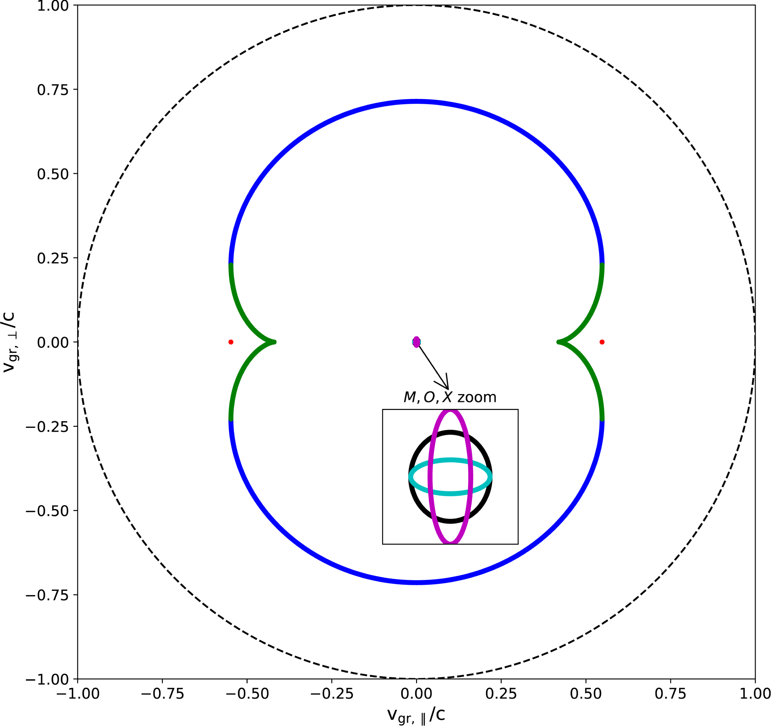
We show in figures 1–3 three typical group diagrams, for parameters
 $E^{2}=10$
and
 $v^{2}=0.3$
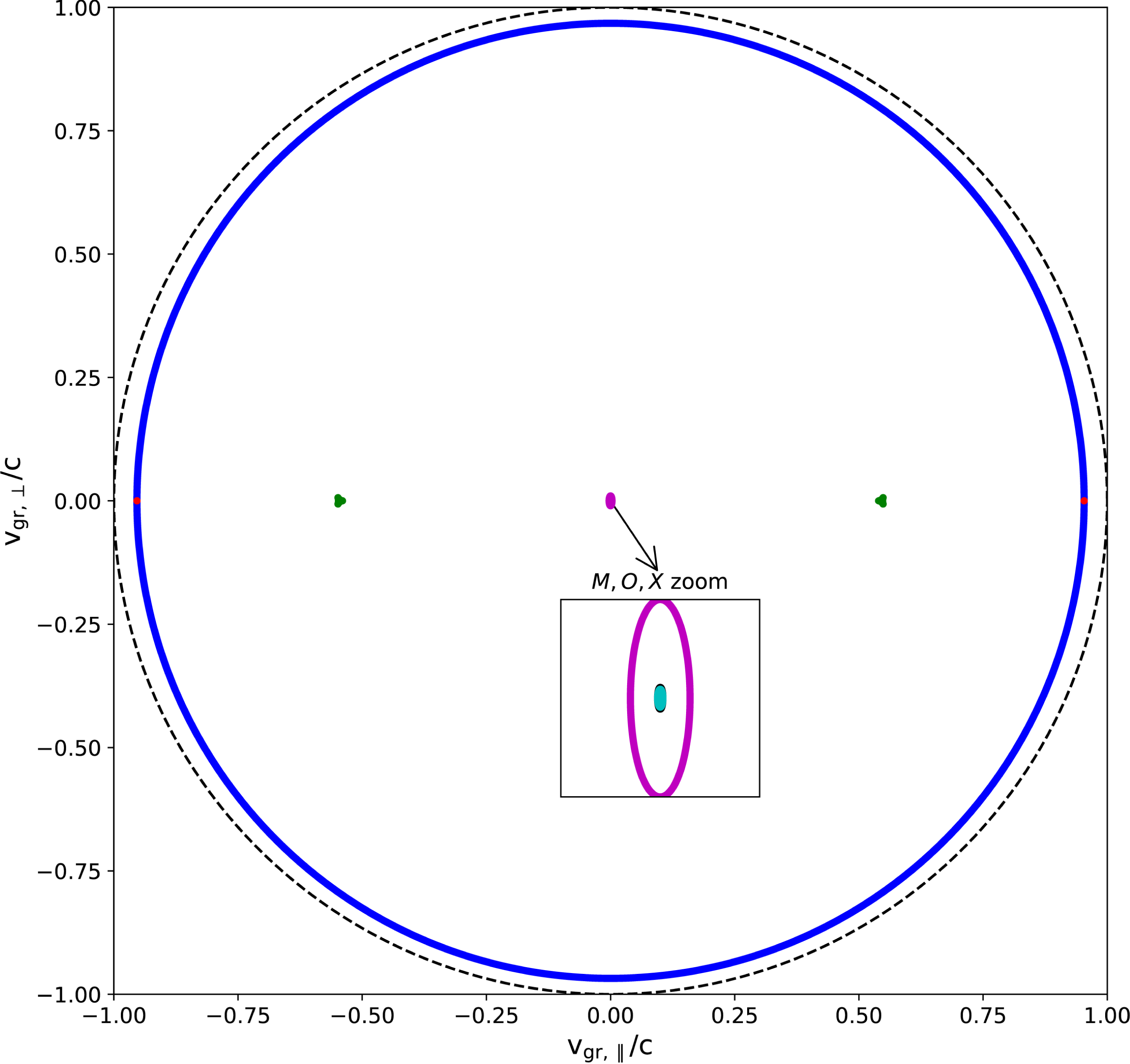
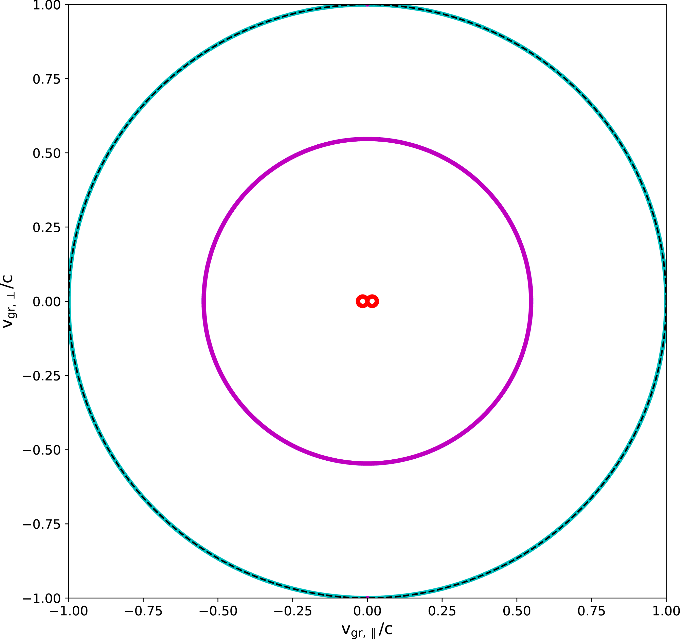
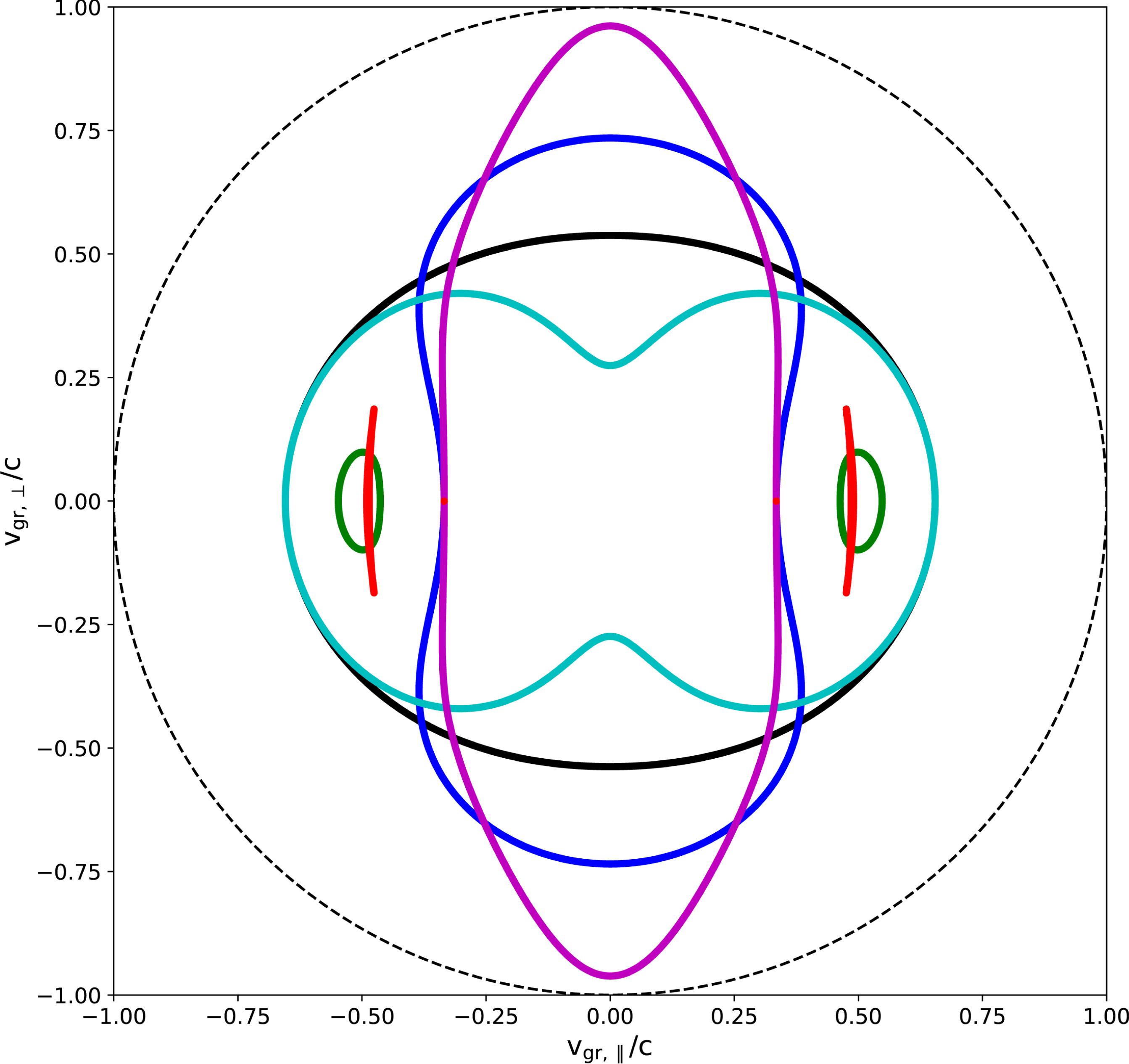
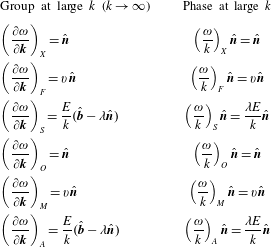
, since these are representative of a highly relativistic regime, both in magnetization and in sound speed. Figure 1 is for long wavelengths, where the relativistic version of the Friedrichs diagram can be recognized for the F (blue), A (red), S (green) modes, where the M (purple), O (cyan) and X (black) modes have small group speeds. In the following section, explicit analytic expressions for this limit are provided. Figure 2 is at short wavelengths, and then the O and X modes essentially give a group speed nearing the light speed (the dashed circle), the M and F modes near the isotropic sound speed circle and the A and S mode show two lobes of forward–backward anisotropic propagation. That in this limit only 3 typical group speed variations are found, is also analytically shown in the next section. At intermediate wavenumbers, fascinating diagrams are obtained that visually show the anisotropy of all wave modes, and figure 3 shows an example at
 $k=3.5$
.
Group diagram for the high magnetization reference case
 $E^{2}=10$
and
 $v^{2}=0.3$
, at long wavelengths (
 $k=0.01$
). In this figure and all the next ones, the following colours are exploited for the X/F/S family: X – black, F – blue, S – green, and for the O/M/A family: O – cyan, M – purple, A – red. The dashed black circle gives the light speed limit. The M, O and X modes all appear near the origin, and are shown in a zoomed fashion in the inset. For this small wavenumber, all modes correspond to their predicted anisotropic limit behaviour from table 1.

Group diagram for the high magnetization reference case
 $E^{2}=10$
and
 $v^{2}=0.3$
, at short wavelengths (
 $k=100$
). Only three curves remain, each is doubly degenerate: the (cyan) O and X modes coincide with the light speed circle, the (purple) M and F modes behave as isotropic sound waves, the (red) A and S modes behave anisotropically. For this large wavenumber, all modes correspond to their predicted anisotropic limit behaviour from table 2.

Group diagram for the high magnetization reference case
 $E^{2}=10$
and
 $v^{2}=0.3$
, at some arbitrary intermediate wavelength (
 $k=3.5$
). The dashed black circle indicates the light speed limit.

6.2 Short and long wavelength limits
Using the knowledge of the cutoffs from (5.1) and the low frequency MHD expressions (4.7), we get immediately the group speed expressions for all six wave modes at long wavelengths (small
 $k$
). Similarly, the resonances from (5.2) as well as the high frequency wave modes from (5.3) provide the six short wavelength limits (large
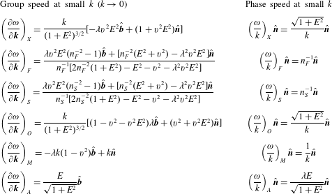
 $k$
). These are collected in tables 1 and 2, for the low and high wavenumbers, respectively. In table 1, we refer to the solutions of (4.5) with
 $n_{S}$
and
 $n_{F}$
, for the slow and fast modes, respectively.
All phase and group speed expressions for all six warm pair plasma wave modes, in the low wavenumber regime.

All phase and group speed expressions for all six warm pair plasma wave modes, in the high wavenumber regime.

A few observations can be made from the expressions listed:
(i) All six wave modes behave anisotropically in their group speed behaviour at large wavelengths. At short wavelengths, only the A and S mode are anisotropic.
(ii) The S, A and F expressions for the group speed variation at low wavenumbers are exactly those known from ideal relativistic MHD. They generalize the well-known Friedrich diagrams to relativistic regimes. They follow directly from the finite
 $n^{2}$
behaviour known for these modes in the low frequency, long wavelength MHD limit.
(iii) At short wavelengths, both electromagnetic O and X modes behave as isotropic light waves. In the same limit, F and M behave as isotropic sound waves.
(iv) These expressions are valid for all combinations of
$E^{2}$
and
$v^{2}$
, and hence contain the special cases of unmagnetized (
$E=0$
) or strongly magnetized (
$E\rightarrow \infty$
) pair plasmas. The cold (
$v=0$
) limit is to be treated differently though, since then the A, M and F modes all have a resonance, while the S branch becomes marginal (Keppens & Goedbloed Reference Keppens and Goedbloed2019b
).


Group diagram for a case where the sound speed (
 $v^{2}=0.3$
) equals the Alfvén speed (i.e.
 $v^{2}=E^{2}/(1+E^{2})$
), at long wavelength (
 $k=0.01$
). The MHD modes S (green), A (red) and F (blue) then show a clearly special topology in this group speed diagram. The other M, O and X modes are also shown in a zoomed in fashion, as they all appear near the origin. For this small wavenumber, all modes agree with the predictions from table 1.

The case where the (squared) sound speed
 $v^{2}$
equals the Alfvén speed
 $E^{2}/(1+E^{2})$
shows an interesting degeneracy, observable in the long wavelength, low frequency MHD limit. Figure 4 shows the group diagram for
 $k=0.01$
, where we took
 $v^{2}=0.3$
and equal to the Alfvén speed. In the next sections, we explain how this degeneracy relates to a special case of avoided crossings of branches.
7 Dispersion diagrams
We now discuss the six branches
 $\unicode[STIX]{x1D714}(k)$
which for a given choice of
 $E^{2}$
and
 $v^{2}$
can be computed at all orientations
 $\unicode[STIX]{x1D706}^{2}\in [0,1]$
. It turns out that the purely parallel (
 $\unicode[STIX]{x1D706}^{2}=1$
) and purely perpendicular (
 $\unicode[STIX]{x1D706}^{2}=0$
) orientations demonstrate degeneracy, which is lifted at arbitrary oblique propagation. Therefore, we discuss oblique propagation first. When showing example figures in what follows, we will always adopt parameters
 $E^{2}=10$
and
 $v^{2}=0.3$
, since these are representative of a highly relativistic regime, both in magnetization and in sound speed.
7.1 Oblique propagation
In the overview of long and short wavelength group speed expressions, we tacitly assumed that the six branches always demonstrate the same connectivity
 $\unicode[STIX]{x1D714}(k)$
between these low and high
 $k$
-limits. At the long wavelength (small
 $k$
) regime, the frequency ordering is always fixed, as the MHD frequencies are ordered and are far below the two cutoffs
 $\unicode[STIX]{x1D714}=1$
and
 $\unicode[STIX]{x1D714}=\sqrt{1+E^{2}}$
. The six wave modes are then also ordered, as
 $\unicode[STIX]{x1D714}_{S}\leqslant \unicode[STIX]{x1D714}_{A}\leqslant \unicode[STIX]{x1D714}_{F}\leqslant \unicode[STIX]{x1D714}_{M}\leqslant \unicode[STIX]{x1D714}_{O}\leqslant \unicode[STIX]{x1D714}_{X}$
. This ordering is maintained at all oblique propagations, a result we also pointed out in the cold pair plasma case (Keppens & Goedbloed Reference Keppens and Goedbloed2019b
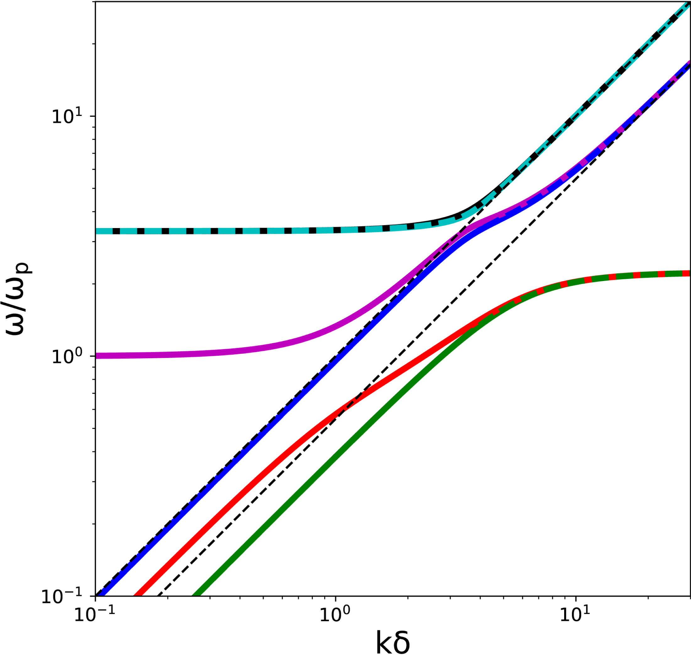
). Figure 5 shows a typical dispersion diagram, containing all six waves at the arbitrary chosen angle of
 $\unicode[STIX]{x1D717}=\unicode[STIX]{x03C0}/4$
. Note how the lower-left corner of this diagram shows us the MHD slow (
 $\unicode[STIX]{x1D714}_{S}$
in green), Alfvén (
 $\unicode[STIX]{x1D714}_{A}$
in red) and fast (
 $\unicode[STIX]{x1D714}_{F}$
in blue) limits. The green and red curves jointly approach the resonance value of
 $\unicode[STIX]{x1D714}=E/\sqrt{2}$
at high wavenumber. At these high wavenumbers, the blue (
 $\unicode[STIX]{x1D714}_{F}$
) and purple (
 $\unicode[STIX]{x1D714}_{M}$
) branches approach the sound wave values, indicated as a dashed black line, while the cyan (
 $\unicode[STIX]{x1D714}_{O}$
) and black (
 $\unicode[STIX]{x1D714}_{X}$
) behave like light waves (also indicated with a dashed black line). The modified electrostatic
 $\unicode[STIX]{x1D714}_{M}$
mode starts off at the plasma frequency, while both electromagnetic modes start off at
 $\sqrt{1+E^{2}}$
. For clarity, the regions where modes seemingly overlap in figure 5 (there are small differences in frequencies at all these limits) show one of the modes using a dashed curve segment. We can produce dispersion diagrams at all angles
 $\unicode[STIX]{x1D717}$
, and then collect the same information in polar plots of phase speed
 $v_{\text{ph}}(\unicode[STIX]{x1D717})=[\unicode[STIX]{x1D714}/k](\unicode[STIX]{x1D703})$
for
 $\unicode[STIX]{x1D717}\in [0,2\unicode[STIX]{x03C0}]$
at a given wavenumber
 $k$
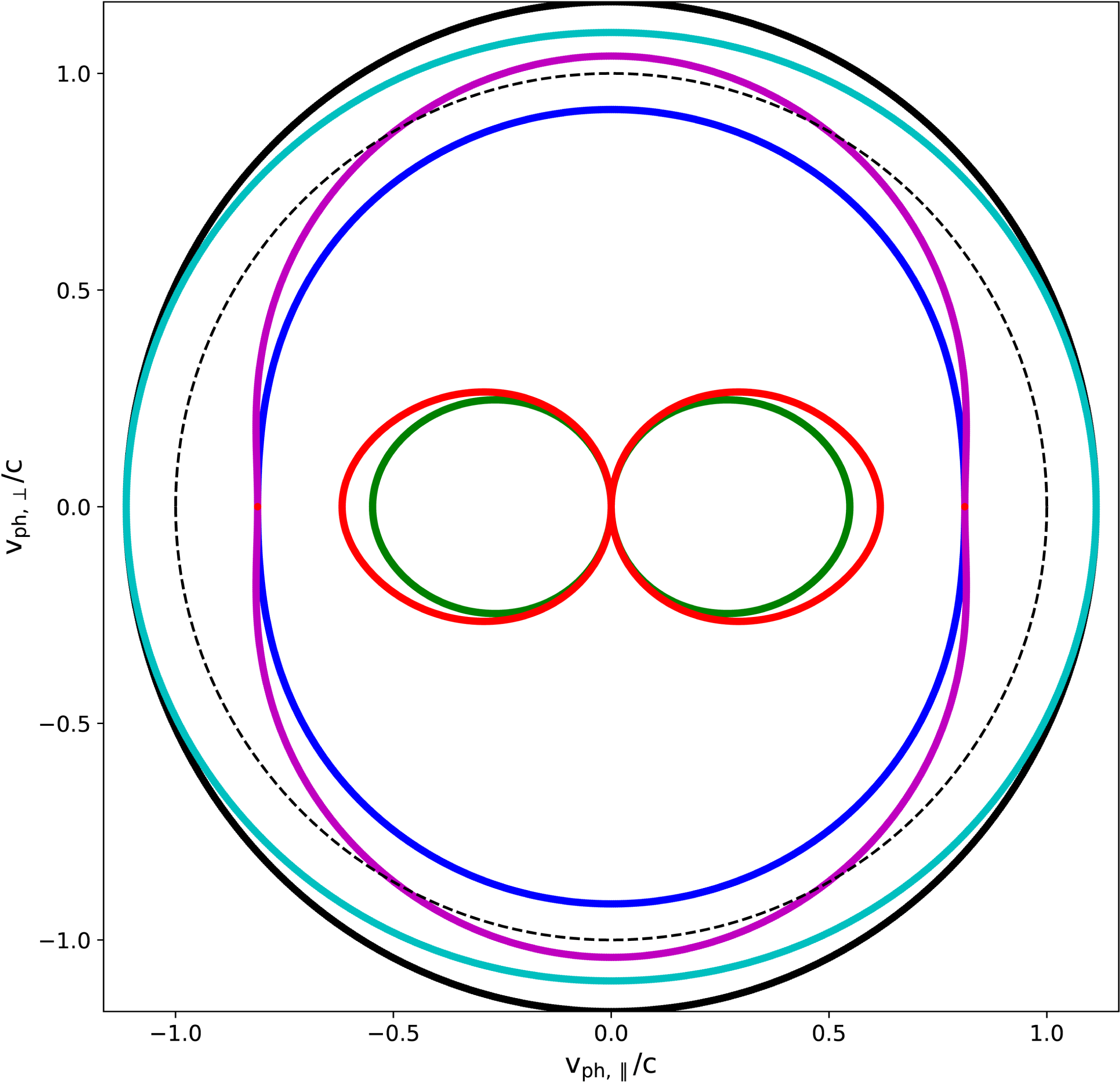
. A typical phase diagram for all six modes is then provided in figure 6, using the same
 $E^{2}=10$
and
 $v^{2}=0.3$
, at
 $k=3.5$
. At this wavenumber value, it is clearly seen how the six modes show nested phase diagrams, while some mode pairs coincide exactly at parallel orientations. This will be discussed in what follows.
A typical dispersion diagram for the reference high magnetization case
 $E^{2}=10$
and
 $v^{2}=0.3$
, at
 $\unicode[STIX]{x1D717}=\unicode[STIX]{x03C0}/4$
. For clarity, the regions where modes seemingly overlap show one of the modes using a dashed curve segment. Slanted black dashed lines correspond to the light speed and sound speed limits.

A typical phase diagram, for the reference high magnetization case
 $E^{2}=10$
and
 $v^{2}=0.3$
at
 $k=3.5$
. The black dashed circle indicates the light speed limit.

We will find that in both the parallel and perpendicular cases the X, F, S and O, M, A families share a common root. This however does not happen for other orientations, as revealed by the resultant. The resultant of two polynomials is a polynomial expression of their coefficients, which is equal to zero if and only if the polynomials have a common root, i.e. a common factor. For the polynomials appearing in (4.1) and (4.2) it reads
 $$\begin{eqnarray}R=-E^{6}k^{6}(1-v^{2})^{2}(1-\unicode[STIX]{x1D706}^{2})^{2}\unicode[STIX]{x1D706}^{2}.\end{eqnarray}$$
Therefore only the
 $\unicode[STIX]{x1D706}=0$
and
 $\unicode[STIX]{x1D706}=1$
orientations lead to common roots between these families.
7.2 Parallel and near-parallel behaviour
If we specify an exactly parallel orientation, we find that both the X, F, S and the O, M, A branches can be factorized completely, as we can write them for
 $\unicode[STIX]{x1D706}=1$
as:
 $$\begin{eqnarray}\displaystyle \left.\begin{array}{@{}rl@{}}\text{X},\text{F},\text{S}: & 0=(\unicode[STIX]{x1D714}^{2}-v^{2}k^{2})[\unicode[STIX]{x1D714}^{4}-(1+E^{2}+k^{2})\unicode[STIX]{x1D714}^{2}+E^{2}k^{2}],\\ \text{O},\text{M},\text{A}: & 0=(\unicode[STIX]{x1D714}^{2}-1-v^{2}k^{2})[\unicode[STIX]{x1D714}^{4}-(1+E^{2}+k^{2})\unicode[STIX]{x1D714}^{2}+E^{2}k^{2}].\end{array}\right\} & & \displaystyle\end{eqnarray}$$
Hence, we find that at parallel orientations only four different branches appear, of which two are doubly degenerate as the quadratic factor in
 $\unicode[STIX]{x1D714}^{2}$
is identical. In the O, M, A family, the
 $\unicode[STIX]{x1D714}^{2}=1+v^{2}k^{2}$
is always the M-branch, as it starts off from the plasma frequency at low
 $k$
, and this mode is the warm pair plasma version of the Langmuir wave discussed in classical plasma physics textbooks. The O and A modes come from the quadratic expression in
 $\unicode[STIX]{x1D714}^{2}$
where the largest frequency is the O mode. This O mode at parallel orientation is always identical to the X mode in the X, F, S branch.
The identification of the F, S modes is more subtle: the square root expression appearing in (4.7) for labelling the S and F branches implies that for
 $\unicode[STIX]{x1D706}=1$
a factor
 $|E^{2}-v^{2}(1+E^{2})|$
appears. This means that the low frequency MHD limit for the F mode will be
 $\unicode[STIX]{x1D714}_{F}^{2}=E^{2}k^{2}/(1+E^{2})$
for
 $E^{2}>v^{2}(1+E^{2})$
and then similarly the low frequency S mode is
 $\unicode[STIX]{x1D714}_{S}^{2}=v^{2}k^{2}$
, but when
 $E^{2}<v^{2}(1+E^{2})$
the labelling changes: F is then
 $\unicode[STIX]{x1D714}_{F}^{2}=v^{2}k^{2}$
. This is well known in MHD, where the changeover at
 $E^{2}=v^{2}(1+E^{2})$
is identifying the field strength value for which the sound speed (
 $v=c_{g}/c$
) coincides with the Alfvén speed
 $v_{A}/c=E/\sqrt{1+E^{2}}$
, or in a Newtonian setting where the plasma beta attains the special value
 $\unicode[STIX]{x1D6FD}=2\unicode[STIX]{x1D707}_{0}p/B^{2}=2/\unicode[STIX]{x1D6FE}$
. We note in passing that the usual MHD phase and Friedrichs wave diagrams indeed contain an interesting degeneracy at precisely this value (see Goedbloed et al. (Reference Goedbloed, Keppens and Poedts2019), chapter 5, their figure 5.4), which we recovered in figure 4 when showing six-mode group diagrams for such a case, in the long wavelength limit.
7.2.1 SF crossings
From (7.2), we can also compute when the S branch intersects with the F branch at parallel orientations. This happens at
 $k$
-values where
 $$\begin{eqnarray}k_{\text{SF}}^{2}=\frac{E^{2}-v^{2}(1+E^{2})}{v^{2}(1-v^{2})},\end{eqnarray}$$
which only correspond to positive values for
 $E^{2}>v^{2}(1+E^{2})$
. Hence, when the Alfvén speed exceeds the sound speed, we will observe a crossing between the S and F branches, at the wavenumber above, and at the frequency given by
 $$\begin{eqnarray}\unicode[STIX]{x1D714}_{\text{SF}}^{2}=E^{2}-\frac{v^{2}}{(1-v^{2})}.\end{eqnarray}$$
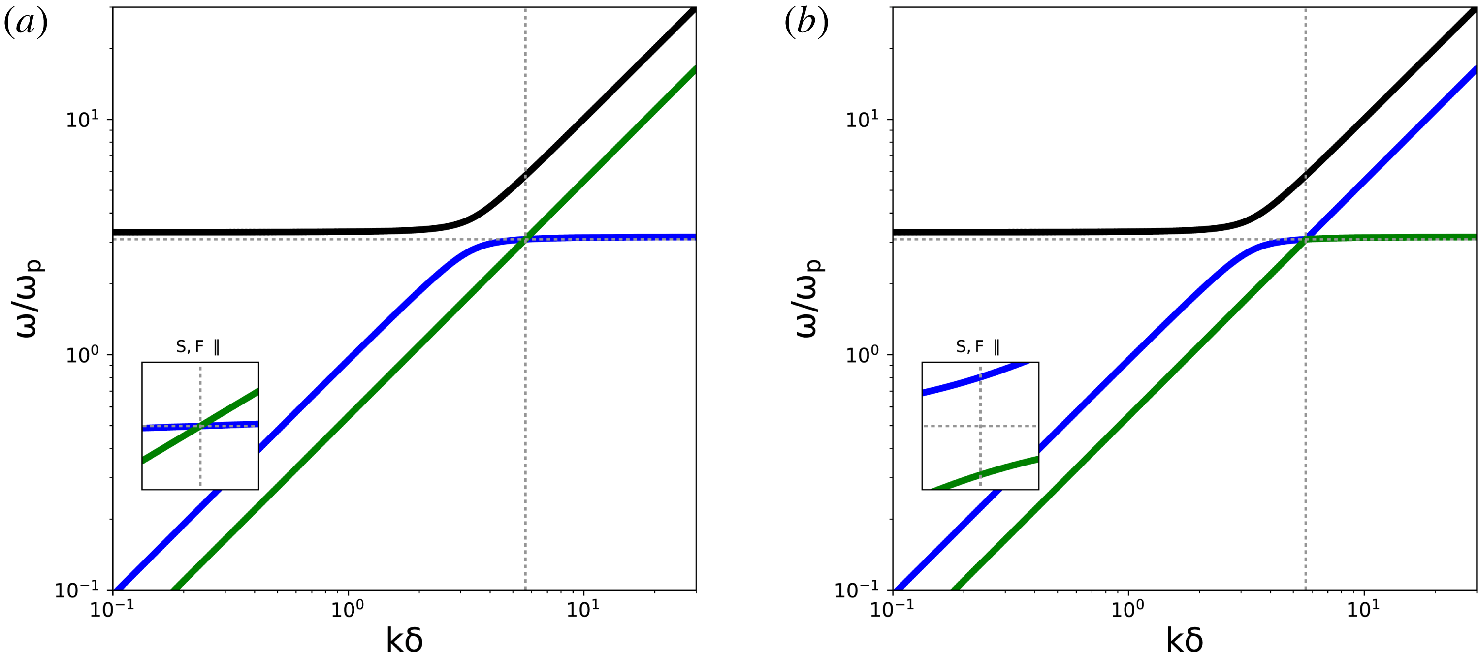
This exact knowledge on when S and F branches cross is relevant to appreciating what happens at near-parallel and all oblique orientations: the branches will demonstrate an avoided crossing, as illustrated in figure 7. In this figure, we only show the X, F and S branches for the
 $E^{2}=10$
and
 $v^{2}=0.3$
case, which indeed is a case where the Alfvén speed exceeds the sound speed. The predicted wavenumber–frequency values for the crossing are indicated with dotted lines. Note the change in connectivity from small to large
 $k$
behaviour for the S and F branches, when going from parallel to near-parallel orientations (we took
 $\unicode[STIX]{x1D717}=0.0005$
for illustration purposes). Note further that in the cold plasma case, the S branch is marginal, and this particular crossing then never occurred.
Dispersion diagram for the X, F, S family, at parallel (a,
 $\unicode[STIX]{x1D717}=0$
) and near-parallel (b,
 $\unicode[STIX]{x1D717}=0.0005$
) orientations for the case
 $E^{2}=10$
and
 $v^{2}=0.3$
. The avoided crossing between the S and F branch is demonstrated in the zoomed inset.

7.2.2 AM crossings
We can further investigate when the A and M branch intersect at parallel orientations. Using (7.2), we find easily that this occurs for wavenumbers obeying
 $$\begin{eqnarray}v^{2}(1-v^{2})k^{4}-(E^{2}-1)(1-v^{2})k^{2}+E^{2}=0.\end{eqnarray}$$
When we consider this for a cold
 $v=0$
pair plasma, there is only one (squared) wavenumber possible namely
 $k^{2}=E^{2}/(E^{2}-1)$
for
 $E>1$
. This crossing was indeed reported in Keppens & Goedbloed (Reference Keppens and Goedbloed2019b
), where the corresponding frequency becomes the plasma frequency. In the cold case, the warm pair Langmuir wave modifies to the purely non-propagating electrostatic mode.
We now see that for a warm pair plasma, we can find two solutions given by
 $$\begin{eqnarray}k_{\text{AM},\pm }^{2}=\frac{(E^{2}-1)(1-v^{2})\pm \sqrt{(1-v^{2})[(E^{2}-1)^{2}-v^{2}(E^{2}+1)^{2}]}}{2v^{2}(1-v^{2})}.\end{eqnarray}$$
The corresponding frequencies are
 $$\begin{eqnarray}\unicode[STIX]{x1D714}_{\text{AM},\pm }^{2}=1+v^{2}k_{\text{AM},\pm }^{2}.\end{eqnarray}$$
In order for both roots
 $k_{\text{AM},\pm }^{2}$
to be positive, we must have
 $E>1$
, as the polynomial (7.5) tells us that their sum
 $k_{\text{AM},+}^{2}+k_{\text{AM},-}^{2}=(E^{2}-1)/v^{2}$
. Also, the expression under the square root in (7.6) requires
 $v^{2}<[(E^{2}-1)/(E^{2}+1)]^{2}$
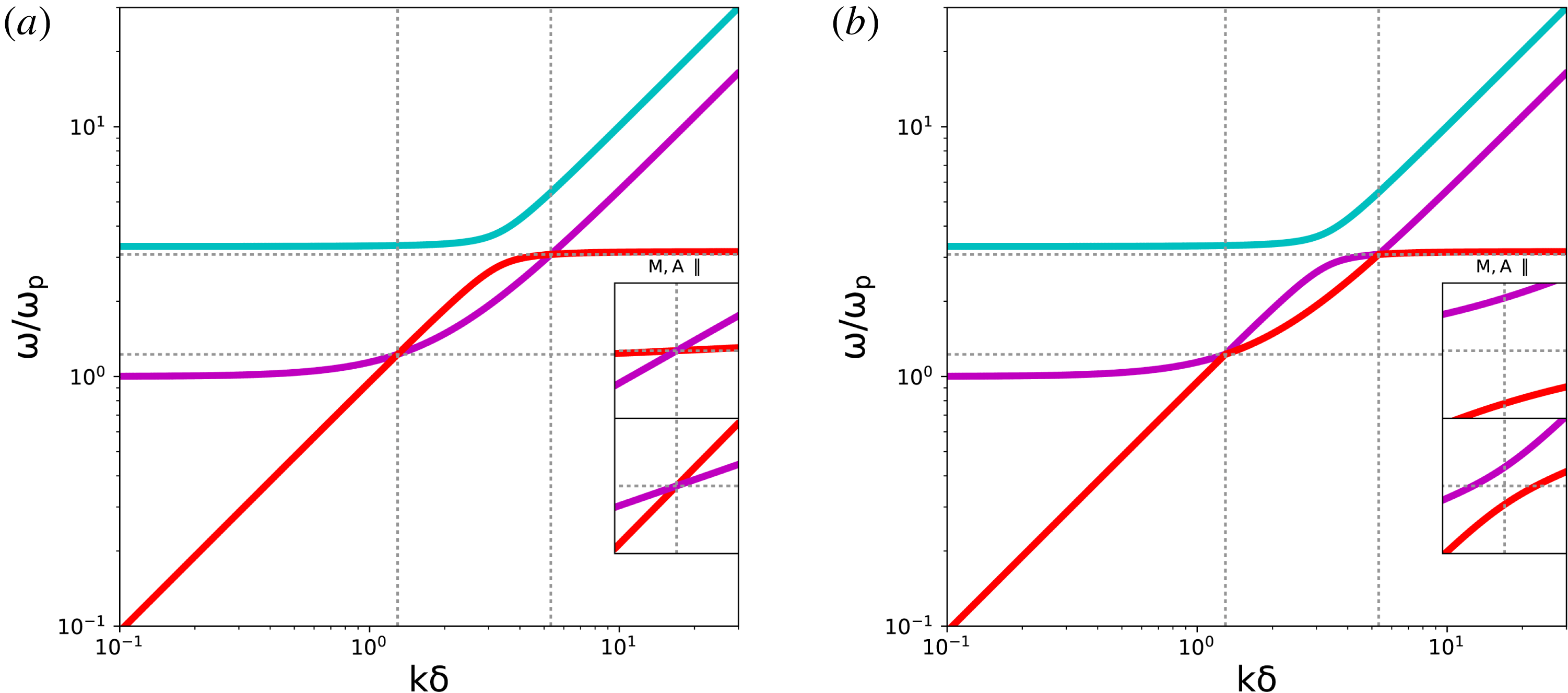
. This is also satisfied for the chosen high magnetization case from the figures, and the double AM crossing is demonstrated in figure 8. At
 $v^{2}=[(E^{2}-1)/(E^{2}+1)]^{2}$
, the Langmuir wave related M branch and the Alfvén branch touch in one point only.
Dispersion diagram for the O, M, A family at parallel (a,
 $\unicode[STIX]{x1D717}=0$
) and near-parallel (b,
 $\unicode[STIX]{x1D717}=0.0005$
) orientations for the case
 $E^{2}=10$
and
 $v^{2}=0.3$
. The double avoided crossing between the A and M branch is demonstrated in the zoomed insets.

7.3 Perpendicular and near-perpendicular behaviour
We can further specify to perpendicular
 $\unicode[STIX]{x1D706}=0$
orientations, where the branches also factorize easily, since then
 $$\begin{eqnarray}\displaystyle \left.\begin{array}{@{}rl@{}}\text{X},\text{F},\text{S}: & 0=\unicode[STIX]{x1D714}^{2}[\unicode[STIX]{x1D714}^{4}-(1+E^{2}+k^{2}+v^{2}k^{2})\unicode[STIX]{x1D714}^{2}+k^{2}(E^{2}+v^{2}+v^{2}k^{2})],\\ \text{O},\text{M},\text{A}: & 0=\unicode[STIX]{x1D714}^{2}(\unicode[STIX]{x1D714}^{2}-1-k^{2})(\unicode[STIX]{x1D714}^{2}-1-E^{2}-v^{2}k^{2}).\end{array}\right\} & & \displaystyle\end{eqnarray}$$
The zero frequency for the first family is the S mode, while it is the A mode for the second family: neither Alfvén nor slow modes propagate perpendicular to the magnetic field. The other modes can be identified without any confusion (M is
 $\unicode[STIX]{x1D714}^{2}=1+k^{2}$
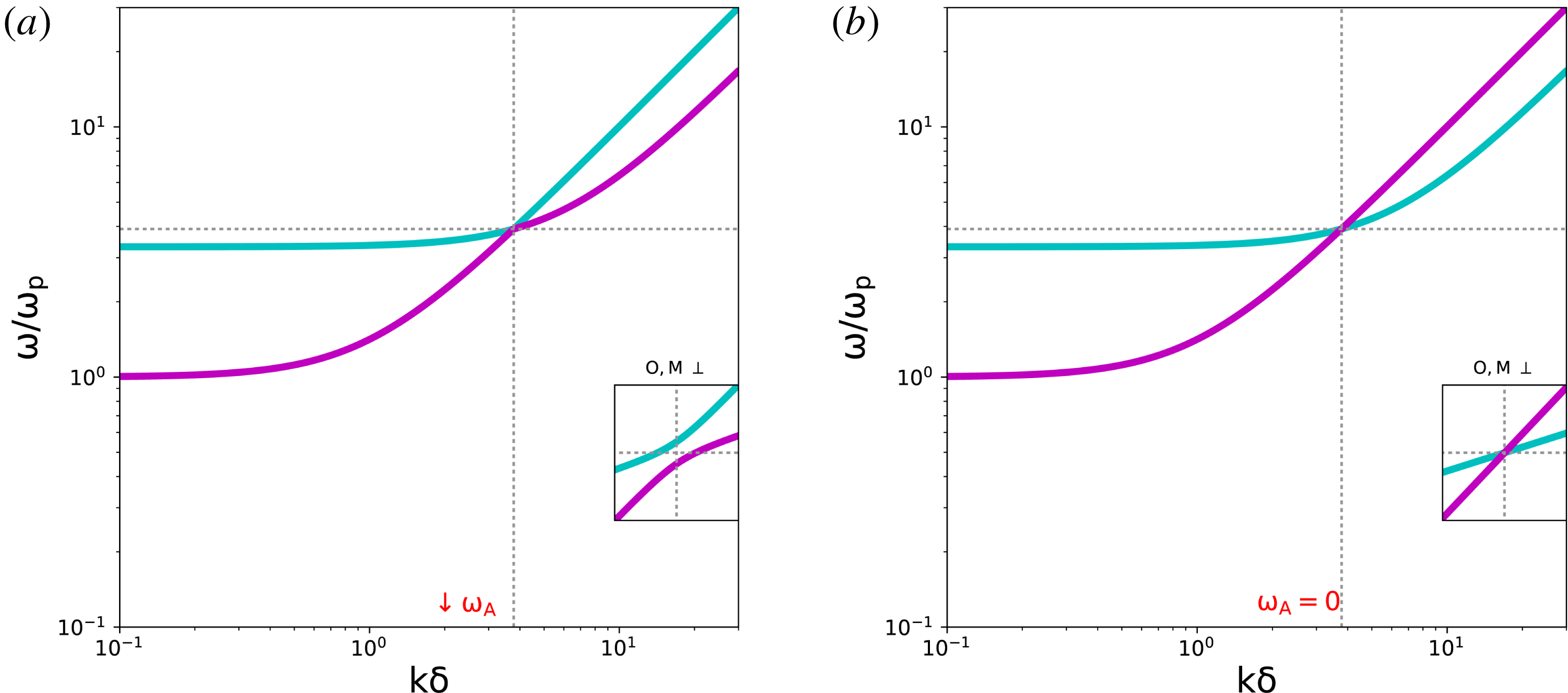
), and it is easily verified that for perpendicular orientations, an unavoidable crossing happens between the O and the M branches, in particular at
 $$\begin{eqnarray}\displaystyle \left.\begin{array}{@{}c@{}}\displaystyle k_{\text{OM}}^{2}=\frac{E^{2}}{1-v^{2}},\\ \displaystyle \unicode[STIX]{x1D714}_{\text{OM}}^{2}=1+\frac{E^{2}}{1-v^{2}}.\end{array}\right\} & & \displaystyle\end{eqnarray}$$
This reduces to the same perpendicular crossing reported for the cold pair plasma case in Keppens & Goedbloed (Reference Keppens and Goedbloed2019b ). At near-perpendicular orientations, the O, M, A family shows the OM crossing as illustrated in figure 9 for our reference high magnetization case. Note once more how the connectivity of the branches between low and high wavenumber regimes clearly changes at exactly perpendicular orientation.
Dispersion diagram for the O, M, A family, at near-perpendicular (
 $\unicode[STIX]{x1D717}=\unicode[STIX]{x03C0}/2-0.0005$
, a) and perpendicular (
 $\unicode[STIX]{x1D717}=\unicode[STIX]{x03C0}/2$
, b) orientations, for the reference high magnetization case
 $E^{2}=10$
and
 $v^{2}=0.3$
. The inset zooms in on the crossing of the O and M branches. The red A mode is off the scale shown, at much lower (or marginal for perpendicular) frequencies.

8 Group diagrams and wave transformations
All the above crossings reported lead to intricate transformations of wave modes, which are particularly evident in group diagrams. The reference high magnetization case was found to demonstrate four of such crossings, at wavenumbers
 $k_{\text{SF}}$
,
 $k_{\text{AM},+}$
,
 $k_{\text{AM},-}$
and at
 $k_{\text{OM}}$
. The SF and AM crossings were found to occur when certain conditions prevail, e.g. when the Alfvén speed is higher than the sound speed we encounter an SF crossing. The near-perpendicular OM crossing always occurs, irrespective of the parameters
 $E^{2}$
and
 $v^{2}$
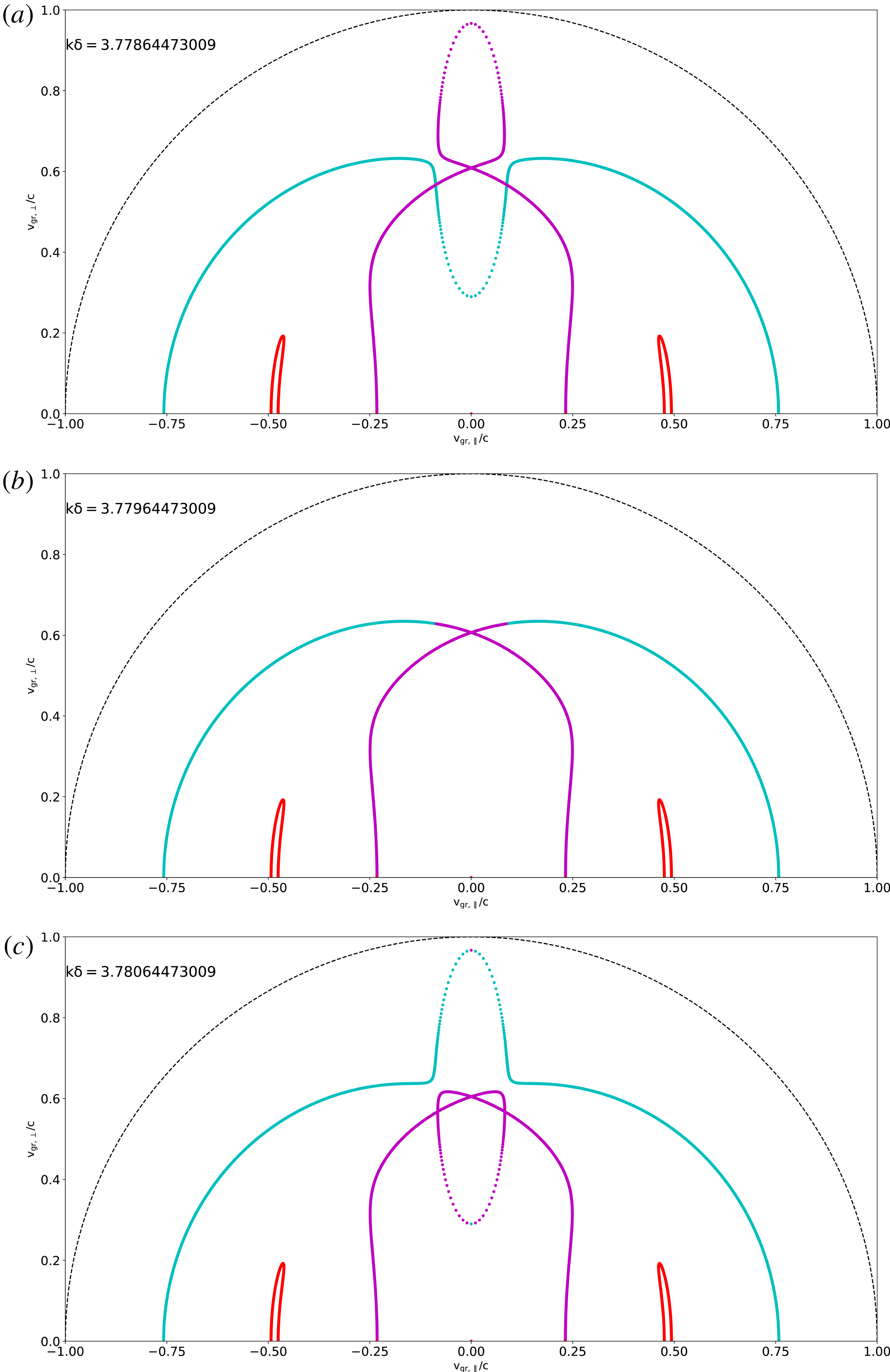
. We therefore illustrate the transformation observed at near-perpendicular orientations in the group diagram, for the reference high magnetization case. Figure 10 shows how the wave anisotropy strikingly changes at precisely the wavenumber–frequency mentioned in (7.9). In the end, an actual exchange of the purely perpendicular solution has occurred between these branches (note the exchanged purple–cyan dot in the bottom panel). The other, near-parallel transformations behave similarly and also exchange purely parallel wave modes between two branches. It is to be expected that these intricate wave transformations have observable consequences in actual warm pair plasmas. Note furthermore that the middle diagram of figure 10 indeed shows a similar topological change as mentioned earlier for the MHD modes, when Alfvén and sound speed coincide (i.e. figure 4).
Group diagram transformation for the case
 $E^{2}=10$
and
 $v^{2}=0.3$
, as one crosses the crossing wavelength
 $k_{\text{OM}}$
for the near-perpendicular OM crossing. We only show the O, M, A family, and take
 $k=k_{\text{OM}}-0.001$
(a),
 $k=k_{\text{OM}}$
(b) and
 $k=k_{\text{OM}}+0.001$
(c). Only half of the group diagram is shown, as there is top–down (and left–right) symmetry.

9 Conclusions
We extended our earlier discussion of waves from the cold pair plasma case (Keppens & Goedbloed Reference Keppens and Goedbloed2019b ) to the warm pair plasma. Using the general polynomial dispersion relation, derived from a symmetrized description of the linear governing equations, we can easily discuss group speed variations, recover their limits at low and high wavenumbers and this for arbitrary orientations between wavevector and magnetic field. The special orientations of parallel and perpendicular propagation are also discussed, but shown to be inappropriate for use as a classification of wave modes types: their variation from low to high wavenumbers is different from any oblique orientation. We argued to be fully consistent with special relativistic MHD, and recovered the MHD Friedrichs diagrams in relativistic conditions (Keppens & Meliani Reference Keppens and Meliani2008). This is illustrated by showing exemplary dispersion curves for a highly magnetized case, which was shown to demonstrate up to four avoided crossings, at precisely known wavenumber–frequency values. We find intricate transformations of the group speed diagrams at near-parallel or near-perpendicular angles, when the wavenumber varies across these predicted wavelengths.
Although complete, our two-fluid treatment shares the usual shortcomings for any fluid viewpoint on plasmas: the subtleties related to velocity phase space resonances (Landau damping, damping of cyclotron wave modes and all intricate instabilities related to some form of anisotropy in the velocity part of the distribution function) are absent. Some aspects can be remedied, e.g. a collisional damping can be incorporated, sometimes as easy as by making the substitution
 $m_{s}\rightarrow m_{s}(1+i\unicode[STIX]{x1D708}_{s}/\unicode[STIX]{x1D714})$
for the mass of species
 $s$
, where a drag force introduces a collision frequency
 $\unicode[STIX]{x1D708}_{s}$
for that species (Gurnett & Bhattacharjee Reference Gurnett and Bhattacharjee2005; Kulsrud Reference Kulsrud2005). This is left for future work, where one should contrast the more complete kinetic dispersion relation with the warm two-fluid limit. For the special case of relevance to pulsar pair plasmas, this comparison is given in appendix B. Aspects to be investigated further are which branches suffer wave–particle-driven damping, where only those parts of the dispersion curves that behave subluminally (phase speeds less than
 $c$
) can be affected.
In the same two-fluid approach, we can do the warm two-fluid analysis for an ion–electron plasma, where the six modes no longer separate into two branches. Then, the intricate mode exchanges are to be studied with more than two parameters: the species can have different temperatures, and the finite mass ratio makes the species cyclotron frequencies differ greatly, so four parameters will need to be varied. It may also be of interest to study the link with single-fluid relativistic resistive MHD wave properties, which have been characterized recently (Mignone, Mattia & Bodo Reference Mignone, Mattia and Bodo2018).
Acknowledgements
This research was supported by the KU Leuven (GOA/2015-014). R.K. thanks Nanjing University and Purple Mountain Observatory for kind hospitality during his sabbatical stay.
Appendix A. Electrostatic versus electromagnetic wave characteristics
The usual textbook approach to plasma wave characterizations often distinguishes between purely electrostatic, versus full electromagnetic wave modes. Electrostatic ones only involve electric field perturbations, i.e. have a perturbed magnetic field
 $$\begin{eqnarray}\unicode[STIX]{x1D714}\tilde{\boldsymbol{B}}=\boldsymbol{k}\times \tilde{\boldsymbol{E}}=\mathbf{0},\end{eqnarray}$$
where the first equality is the Fourier form of Ampère’s law, and the last is specific for electrostatic waves. Waves which do involve perturbed magnetic fields are termed electromagnetic.
In § 3, we explained how the six-mode dispersion relation follows from a
 $6\times 6$
real symmetric matrix formulation, adopting a specific scaling and choice for the linear quantities retained, as given by (3.4). As we retained two components of the electric field, namely
 $\tilde{E}_{1}$
in the
 $\boldsymbol{k}{-}\boldsymbol{B}$
plane perpendicular to
 $\boldsymbol{k}$
, and
 $\tilde{E}_{2}$
perpendicular to the
 $\boldsymbol{k}{-}\boldsymbol{B}$
plane, electrostatic modes must make both of these perturbations zero. Electrostatic modes indeed only have
 $\boldsymbol{k}$
aligned electric field perturbations, i.e. only non-vanishing
 $\tilde{E}_{3}$
components, which we conveniently removed from our analysis. Actually, it is easy to show that
 $\tilde{E}_{3}\propto \tilde{U} _{e3}-\tilde{U} _{p3}$
, so its value is directly available from the retained velocity components.
Electromagnetic modes then correspond to any mode which has either one of
 $\tilde{E}_{1}$
or
 $\tilde{E}_{2}$
non-vanishing. Note further that due to the divergence constraint,
 $\tilde{B}_{3}=0$
always, hence it was also removed from the formulation. At this point, we can exploit the real–symmetric nature of the matrix and compute its six real eigenvalues and the corresponding set of mutually orthogonal eigenvectors. This can be done using computer algebra software, and we provide expressions for the specific cases of purely parallel (
 $\unicode[STIX]{x1D717}=0$
or
 $\unicode[STIX]{x1D706}=1$
) or purely perpendicular (
 $\unicode[STIX]{x1D717}=\unicode[STIX]{x03C0}/2$
) propagation.
For parallel propagation, when introducing
 $$\begin{eqnarray}\displaystyle & \unicode[STIX]{x1D6E5}_{1}=\sqrt{(1+E^{2}+k^{2})^{2}-4E^{2}k^{2}}, & \displaystyle\end{eqnarray}$$
 $$\begin{eqnarray}\displaystyle & \unicode[STIX]{x1D6E5}_{2}=\sqrt{4\unicode[STIX]{x1D714}^{2}+(E^{2}-k^{2})^{2}}, & \displaystyle\end{eqnarray}$$
the six eigenvalue eigenvectors are
 $$\begin{eqnarray}\displaystyle \unicode[STIX]{x1D714}^{2}-k^{2}v^{2}, & & \displaystyle (0,0,0,1,0,1)^{\text{T}},\end{eqnarray}$$
 $$\begin{eqnarray}\displaystyle \unicode[STIX]{x1D714}^{2}-1-k^{2}v^{2}, & & \displaystyle (0,0,0,-1,0,1)^{\text{T}},\end{eqnarray}$$
 $$\begin{eqnarray}\displaystyle \unicode[STIX]{x1D714}^{2}-{\textstyle \frac{1}{2}}(1+E^{2}+k^{2})-{\textstyle \frac{1}{2}}\unicode[STIX]{x1D6E5}_{1}, & & \displaystyle \left(0,\frac{-1+E^{2}-k^{2}-\unicode[STIX]{x1D6E5}_{1}}{E\sqrt{2}},1,0,1,0\right)^{\!\text{T}},\end{eqnarray}$$
 $$\begin{eqnarray}\displaystyle \unicode[STIX]{x1D714}^{2}-{\textstyle \frac{1}{2}}(1+E^{2}+k^{2})+{\textstyle \frac{1}{2}}\unicode[STIX]{x1D6E5}_{1}, & & \displaystyle \left(0,\frac{-1+E^{2}-k^{2}+\unicode[STIX]{x1D6E5}_{1}}{E\sqrt{2}},1,0,1,0\right)^{\!\text{T}},\end{eqnarray}$$
 $$\begin{eqnarray}\displaystyle \unicode[STIX]{x1D714}^{2}-{\textstyle \frac{1}{2}}(E^{2}+k^{2})-{\textstyle \frac{1}{2}}\unicode[STIX]{x1D6E5}_{2}, & & \displaystyle \left(\frac{-E^{2}+k^{2}+\unicode[STIX]{x1D6E5}_{2}}{\sqrt{2\unicode[STIX]{x1D714}^{2}}},0,-1,0,1,0\right)^{\!\text{T}},\end{eqnarray}$$
 $$\begin{eqnarray}\displaystyle \unicode[STIX]{x1D714}^{2}-{\textstyle \frac{1}{2}}(E^{2}+k^{2})+{\textstyle \frac{1}{2}}\unicode[STIX]{x1D6E5}_{2}, & & \displaystyle \left(\frac{-E^{2}+k^{2}-\unicode[STIX]{x1D6E5}_{2}}{\sqrt{2\unicode[STIX]{x1D714}^{2}}},0,-1,0,1,0\right)^{\!\text{T}}.\end{eqnarray}$$
Comparing these expressions for the eigenvalues of the matrix with the specific factorization (7.2) of the dispersion relation obtained for parallel propagation, we can note:
(i) The vanishing of the first matrix eigenvalue (A 4) leads to
$\unicode[STIX]{x1D714}^{2}=v^{2}k^{2}$
, which is the S or F branch depending on the ratio of sound to Alfvén speed. The corresponding eigenvector has no electromagnetic perturbations (i.e. we have
$\tilde{E}_{1}=0=\tilde{E}_{2}$
, but also
$\tilde{E}_{3}\propto \tilde{U} _{e3}-\tilde{U} _{p3}$
vanishes), and is a pure sound wave with associated density–pressure perturbations. The velocity perturbation for electrons and positrons has a component along
$\boldsymbol{k}$
, where they move in phase (i.e. we have
$\tilde{U} _{e3}=\tilde{U} _{p3}$
). This branch was not even mentioned in Stewart & Laing (Reference Stewart and Laing1992).(ii) The vanishing of the second matrix eigenvalue (A 5) leads to the M branch. As
$\tilde{E}_{1}=0=\tilde{E}_{2}$
, but
$\tilde{E}_{3}\neq 0$
, this branch is purely electrostatic (no magnetic perturbations) and is the textbook Langmuir wave. The velocity perturbation for electrons and positrons has a component along
$\boldsymbol{k}$
, where they move out of phase.(iii) The vanishing of the third matrix eigenvalue (A 6) gives us the coincident O and X mode. This mode is electromagnetic (only
$\tilde{E}_{2}\neq 0$
), and there is no associated movement of electrons and positrons along
$\boldsymbol{k}$
(implying no density or pressure perturbations, and a transverse wave character).(iv) The vanishing of the fourth matrix eigenvalue (A 7) gives us the coincident A and S or F modes (the latter choice again depending on plasma beta). This mode is electromagnetic, and there is no associated movement of electrons and positrons along
$\boldsymbol{k}$
.(v) The vanishing of the remaining two matrix eigenvalues also corresponds to the shared quadratic factor
$\unicode[STIX]{x1D714}^{4}-\unicode[STIX]{x1D714}^{2}(1+E^{2}+k^{2})+E^{2}k^{2}=0$
from (7.2), i.e. the degeneracy of the branches found at parallel orientations.



For the perpendicular case, we can also list the eigenvalue eigenvectors. Introducing
 $$\begin{eqnarray}\displaystyle & \unicode[STIX]{x1D6E5}_{3}=\sqrt{(1+E^{2}+k^{2}+v^{2}k^{2})^{2}-4k^{2}(E^{2}+v^{2}+v^{2}k^{2})}, & \displaystyle\end{eqnarray}$$
 $$\begin{eqnarray}\displaystyle & \unicode[STIX]{x1D6E5}_{4}=\sqrt{k^{4}+4\unicode[STIX]{x1D714}^{2}}, & \displaystyle\end{eqnarray}$$
these become
 $$\begin{eqnarray}\displaystyle \unicode[STIX]{x1D714}^{2}, & & \displaystyle (0,0,1,0,1,0)^{\text{T}},\end{eqnarray}$$
 $$\begin{eqnarray}\displaystyle \unicode[STIX]{x1D714}^{2}-1-E^{2}-v^{2}k^{2}, & & \displaystyle (0,0,0,-1,0,1)^{\text{T}},\end{eqnarray}$$
 $$\begin{eqnarray}\displaystyle \unicode[STIX]{x1D714}^{2}-{\textstyle \frac{1}{2}}(1+E^{2}+k^{2}+v^{2}k^{2})-{\textstyle \frac{1}{2}}\unicode[STIX]{x1D6E5}_{3}, & & \displaystyle \left(0,\frac{-1+E^{2}-k^{2}+k^{2}v^{2}-\unicode[STIX]{x1D6E5}_{3}}{E\sqrt{2}},0,1,0,1\right)^{\!\text{T}}\!,\quad \nonumber\\ \displaystyle & & \displaystyle\end{eqnarray}$$
 $$\begin{eqnarray}\displaystyle \unicode[STIX]{x1D714}^{2}-{\textstyle \frac{1}{2}}(1+E^{2}+k^{2}+v^{2}k^{2})+{\textstyle \frac{1}{2}}\unicode[STIX]{x1D6E5}_{3}, & & \displaystyle \left(0,\frac{-1+E^{2}-k^{2}+k^{2}v^{2}+\unicode[STIX]{x1D6E5}_{3}}{E\sqrt{2}},0,1,0,1\right)^{\!\text{T}}\!,\quad \nonumber\\ \displaystyle & & \displaystyle\end{eqnarray}$$
 $$\begin{eqnarray}\displaystyle \unicode[STIX]{x1D714}^{2}-{\textstyle \frac{1}{2}}k^{2}-{\textstyle \frac{1}{2}}\unicode[STIX]{x1D6E5}_{4}, & & \displaystyle \left(\frac{k^{2}+\unicode[STIX]{x1D6E5}_{4}}{\sqrt{2\unicode[STIX]{x1D714}^{2}}},0,-1,0,1,0\right)^{\!\text{T}},\end{eqnarray}$$
 $$\begin{eqnarray}\displaystyle \unicode[STIX]{x1D714}^{2}-{\textstyle \frac{1}{2}}k^{2}+{\textstyle \frac{1}{2}}\unicode[STIX]{x1D6E5}_{4}, & & \displaystyle \left(\frac{k^{2}-\unicode[STIX]{x1D6E5}_{4}}{\sqrt{2\unicode[STIX]{x1D714}^{2}}},0,-1,0,1,0\right)^{\!\text{T}}.\end{eqnarray}$$
These can again be identified with the branches noted in (7.8), noting that this time the
 $\unicode[STIX]{x1D714}^{2}=1+E^{2}+v^{2}k^{2}$
(i.e. the O branch) behaves electrostatic (
 $\tilde{E}_{3}\neq 0$
, in Stewart & Laing (Reference Stewart and Laing1992) these are called ‘a magnetized analogue of Langmuir waves’, corresponding to plasma upper-hybrid waves), and the marginal frequency
 $\unicode[STIX]{x1D714}^{2}=0$
(as the S branch, omitted in Stewart & Laing (Reference Stewart and Laing1992)) has no electromagnetic perturbations. The vanishing of eigenvalues (A 16)–(A 17) occurs for
 $(\unicode[STIX]{x1D714}^{2}-1-k^{2})\unicode[STIX]{x1D714}^{2}=0$
(i.e. the M and A branches). Note that at this perpendicular orientation, the M mode has
 $\tilde{E}_{1}\neq 0$
, making it a transverse electromagnetic wave.
At intermediate angles, we may similarly get explicit expressions for the eigenvalue–eigenvector pairs. It is already clear from the above special orientations that the M branch (for modified electrostatic) is not always electrostatic, while the ‘electromagnetic’ O mode can indeed become electrostatic (e.g. at perpendicular orientations). The mode nature is thus mixed when the angle gets varied, and we therefore prefer the unambiguous naming scheme S, A, F, M, O and X.
Appendix B. Pulsar relevant limit
Wave dispersion of strongly magnetized pair plasmas is of significant interest in astrophysical context, especially for pulsars, where the typical radio emission has been attributed to various mechanisms (see, e.g. Arons & Barnard Reference Arons and Barnard1986; Rafat et al. Reference Rafat, Melrose and Mastrano2019). Since the work by Arons & Barnard (Reference Arons and Barnard1986), deriving dispersion relations for normal modes in (ultra)relativistically streaming pair plasmas in superstrong magnetic fields, it became customary to focus on the low frequency assumption, i.e. those modes whose Doppler shifted wave frequencies are much below the cyclotron frequency (see, e.g. Lyutikov Reference Lyutikov1998; Rafat et al. Reference Rafat, Melrose and Mastrano2019). At the same time, these fully kinetic treatments of the retained normal modes quantify effects of e.g. Landau damping, invariably invoking transcendental functions (the relativistic plasma dispersion function) to handle the potential wave–particle resonances. Such effects are fully ignored in the ideal two-fluid treatments, where the dispersion relation becomes a simple polynomial expression. However, we will now demonstrate the relevance of both the cold and the warm two-fluid viewpoints on wave dispersion in pair plasmas, as presented in Keppens & Goedbloed (Reference Keppens and Goedbloed2019b ) and in this paper, respectively.
We first focus on the cold pair plasma case, where our previous work (Keppens & Goedbloed Reference Keppens and Goedbloed2019b
) identified two decoupled sets of modes given by the
 $v=0$
limit of (4.1)–(4.2), which we can reorganize into the following expressions:
 $$\begin{eqnarray}\displaystyle & \displaystyle n^{2}=1-\frac{1}{\unicode[STIX]{x1D714}^{2}-E^{2}}, & \displaystyle\end{eqnarray}$$
 $$\begin{eqnarray}\displaystyle & \displaystyle n^{2}=\frac{(\unicode[STIX]{x1D714}^{2}-1)(\unicode[STIX]{x1D714}^{2}-1-E^{2})}{\unicode[STIX]{x1D706}^{2}E^{2}+\unicode[STIX]{x1D714}^{2}(\unicode[STIX]{x1D714}^{2}-1-E^{2})}. & \displaystyle\end{eqnarray}$$
These two branches, which contain our X and F modes in (B 1), and our O, M and A modes in (B 2), are in exact correspondence with expressions in Lyutikov (Reference Lyutikov1999) (in the extended preprint physics/9807022, his (11)–(12)), or in Stewart & Laing (Reference Stewart and Laing1992) (their (15)). The limit of infinite magnetic field implies
 $E\rightarrow \infty$
, and hence retains only one mode from the first branch, and two modes from the second one, which obey
 $$\begin{eqnarray}\displaystyle & \unicode[STIX]{x1D714}^{2}-k^{2}=0, & \displaystyle\end{eqnarray}$$
 $$\begin{eqnarray}\displaystyle & \unicode[STIX]{x1D714}^{4}-\unicode[STIX]{x1D714}^{2}(1+k^{2})+k^{2}\unicode[STIX]{x1D706}^{2}=0. & \displaystyle\end{eqnarray}$$
Which modes of the original five (X, F, O, M and A) are retained is easily identified, since both our X and O modes have cutoff
 $k\rightarrow 0$
behaviour given by
 $\unicode[STIX]{x1D714}^{2}=1+E^{2}$
, so they moved off to infinity, making the F mode approach the light behaviour given by (B 3), while the M and A modes remain in (B 4). This is in perfect agreement with the corresponding limits as identified in Arons & Barnard (Reference Arons and Barnard1986), where our (B 4) is identical to their (50). Their (50) refers to the infinite magnetic field limit of the ‘ordinary’ or O-mode branch, obtained from a fully kinetic description where a delta-function distribution is inserted, and where one expresses the dispersion relation in the rest frame of the plasma. The
 $n^{2}=1$
mode recovers the exact behaviour for the ‘extraordinary’ or X-mode, as found from the infinite magnetic field limit of (83) in Arons & Barnard (Reference Arons and Barnard1986). The main source of potential confusion is that this mode is not our X mode, but our F mode in the strong field limit.
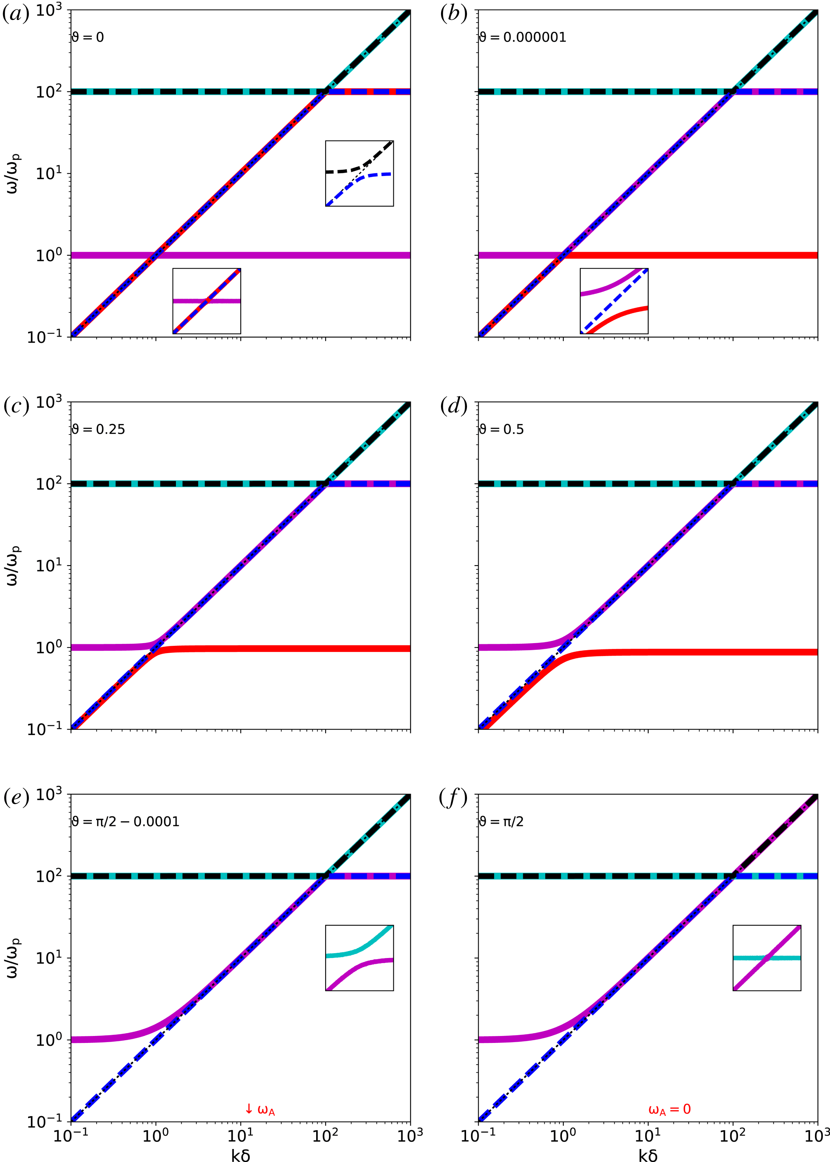
The cold plasma dispersion diagram for six different orientations, in a strongly magnetized
 $E=100$
case as relevant for pulsar physics. All panels show all five modes, in the usual colour coding, but the angle independent X (black) and F (blue) modes are shown in dashes, so overlap of modes can be better appreciated. Note that these X and F modes never cross, as indicated in the upmost inset for parallel orientations. The four upper panels show the typical changeover from parallel to oblique for the M (purple) and A (red) mode, known from the low frequency limit of pulsar theory. Important is the high frequency behaviour when approaching perpendicular orientations (e,f), where the A mode is off the scale shown but where the O and M modes show a similar interaction (as shown in insets).

The advantage of our two-fluid viewpoint is that we do not need to focus solely on the three low frequency modes (F, M and A) retained in the cold, strong field limit, but can demonstrate what happens with all five modes, including the actual high frequency electromagnetic counterpart waves, which are our X and O modes. In figure 11, we show dispersion relations for all five modes (we took
 $E=100$
in this figure), for six different orientations varying from
 $\unicode[STIX]{x1D717}=0$
(parallel),
 $\unicode[STIX]{x1D717}=0.000001$
,
 $\unicode[STIX]{x1D717}=0.25$
and
 $\unicode[STIX]{x1D717}=0.5$
, to
 $\unicode[STIX]{x1D717}=\unicode[STIX]{x03C0}/2-0.0001$
and
 $\unicode[STIX]{x1D717}=\unicode[STIX]{x03C0}/2$
(perpendicular). For visualization purposes, the X and F modes are shown in dashed black and blue lines, and these branches are angle independent for a cold pair plasma. The other modes are shown in the colour coding we used before: red for A, cyan for O and purple for M. At exactly parallel orientation (a), the M branch reduces to
 $\unicode[STIX]{x1D714}=1$
, which crosses the coincident A and F modes at a predictable frequency (see also Arons & Barnard (Reference Arons and Barnard1986), their figure 1, or Rafat et al. (Reference Rafat, Melrose and Mastrano2019), their figure 5, or also shown in Lyutikov (Reference Lyutikov1999), his figure 2). In that orientation, also the O and X modes coincide, as noted in Keppens & Goedbloed (Reference Keppens and Goedbloed2019b
), but these two modes are never retained in works employing the low frequency assumption. In the top right panel, we show what happens at near-parallel behaviour, and indeed we recover the avoided crossing as shown in the lower insets, where suddenly the A mode shows a different resonance from the F mode. Following the behaviour of the M and A modes for varying angles, we get the very same behaviour as discussed in Rafat et al. (Reference Rafat, Melrose and Mastrano2019), where one must be aware of the different names employed there: their X mode is our F, and their L and A modes are the M and A modes used here. In our two-fluid picture, we can follow the high frequency behaviour of these modes, and find that at all orientations, the F mode shows a cyclotron resonance towards
 $\unicode[STIX]{x1D714}=E$
, and the angle-independent F and X modes never cross, as illustrated in the second inset in the top left panel (note that the enormous range in frequencies and wavenumbers displayed shows some misleading apparent crossings, and only zoomed views demonstrate the true behaviour). In contrast, the angle-dependent O (cyan) and M (purple) modes do finally cross at exactly perpendicular orientation, as shown in the insets in the bottom two panels. That in particular the M mode can ultimately transform to a true light wave at perpendicular orientation may be very relevant to pulsar emission.
While the cold two-fluid limit is thus clearly related to the low frequency approximation for normal modes in superstrong magnetic fields, there are various dispersion relation aspects that differ. If we translate the results from Rafat et al. (Reference Rafat, Melrose and Mastrano2019) to our notation, their low frequency, non-gyrotropic approximation yields (in the pulsar rest frame),
 $$\begin{eqnarray}\displaystyle & \displaystyle \unicode[STIX]{x1D714}^{2}=k^{2}\frac{(E^{2}-\unicode[STIX]{x1D706}^{2}v_{\Vert }^{2})}{1+E^{2}},\qquad & \displaystyle\end{eqnarray}$$
 $$\begin{eqnarray}\displaystyle & \displaystyle \unicode[STIX]{x1D714}^{4}-\unicode[STIX]{x1D714}^{2}\left[\unicode[STIX]{x1D714}_{L}^{2}+k^{2}(E^{2}-v_{\Vert }^{2})\left(\frac{1}{E^{2}}+\unicode[STIX]{x1D706}^{2}\left(\frac{1}{1+E^{2}}-\frac{1}{E^{2}}\right)\right)\right]=-k^{2}\unicode[STIX]{x1D706}^{2}\unicode[STIX]{x1D714}_{L}^{2}\frac{(E^{2}-v_{\Vert }^{2})}{1+E^{2}}.\qquad & \displaystyle\end{eqnarray}$$
The first of these expressions is the X-mode (our F mode), and agrees with the corresponding (83) in Arons & Barnard (Reference Arons and Barnard1986), where the indication
 $v_{\Vert }$
results from considering only parallel thermal motion, justified by the highly anisotropic (velocity) distribution expected in superstrong magnetic fields. This split into parallel versus perpendicular pressures could be accounted for in an extended two-fluid picture, introducing potential firehose instabilities. In fact, in the extreme anisotropy expected in a pulsar magnetosphere, one may argue for a zero perpendicular pressure (often used in kinetic treatments when assuming the delta-function distribution in perpendicular velocity) while only a parallel pressure remains. The latter (B 6) combines the L and A modes (our M and A) from Rafat et al. (Reference Rafat, Melrose and Mastrano2019), but is more involved due to the appearance of the relativistic plasma dispersion function, making
 $\unicode[STIX]{x1D714}_{L}^{2}$
a complex, transcendental function of
 $z\equiv \unicode[STIX]{x1D714}/(\unicode[STIX]{x1D706}k)$
. The latter involves integrations accounting for pole contributions, with an assumed distribution function, which was taken as a one-dimensional Juttner distribution, for which the cold limit makes
 $\unicode[STIX]{x1D714}_{L}^{2}\rightarrow 1$
(and
 $v_{\Vert }\rightarrow 0$
). On visual inspection, these expressions differ from our warm (and cold) two-fluid results. The point to note is that the function
 $\unicode[STIX]{x1D714}_{L}^{2}$
can behave such that in relativistically hot regimes, the latter branch becomes multivalued in its L mode, and can introduce an additional lower frequency branch. It is tempting to relate this with the appearance of the S mode, as present in the two-fluid picture. A fourth low frequency mode is also retained in Lyutikov (Reference Lyutikov1998), where it is called the ‘slow Alfvén mode’, and which can be expected to correspond exactly to the S mode (as it also belongs to the X, F, S family). The differences between (B 5)–(B 6) and our expressions for the warm two-fluid mode families should be studied in future work. We note that our two-fluid results recover the exact relativistic versions of the MHD modes, and this is not the case for the results shown above. In particular, the MHD expressions for the F, A and S modes never have superluminal phase speeds, only the M, O and X modes show this possibility, while Lyutikov (Reference Lyutikov1998) reports the possibility of superluminous fast transverse waves. Finally, our expressions recover all limits properly, e.g. the unmagnetized case
 $E=0$
, which is obviously not described by (B 6).