Ethnic diversity is widely held to make governance more difficult. Such diversity is associated with low production of public goods; poor economic growth; and high levels of corruption, violence, and civil conflict. But diversity hardly sentences a country to poor political and economic outcomes. Latvia, for example, has better governance indicators than Brazil, and Zambia has better governance indicators than Nigeria, even though these pairs of countries have similar levels of ethnolinguistic fractionalization (ELF). Why, then, do some countries cope more successfully with ethnic diversity than others?

This article addresses this question by focusing on the nature of substantive differences between groups. The vast majority of cross-national evidence about ethnic diversity and governance uses the standard measure of ELF (e.g., Alesina et al. Reference Alesina, Devleeschauwer, Easterly, Kurlat and Wacziarg2003; Alesina and La Ferrara Reference Alesina and La Ferrara2005; Collier Reference Collier2000; Easterly and Levine Reference Easterly and Levine1997; La Porta et al. Reference La Porta, Lopez-de-Silanes, Shleifer and Vishny1999). This measure contains information about the identity and size of groups but incorporates no other information about groups' substantive characteristics. Existing arguments about how ethnic diversity affects governance, however, are typically grounded in the assumption that groups differ from each other in substantively important ways, and posit that these differences underlie governance problems in multiethnic societies.

This article examines two important types of differences between groups—cultural and economic. Our goal is to understand the empirical relationship between such differences and public goods provision across countries. Is diversity more problematic for governance in countries when this diversity is based on strong cultural or economic differences between groups? Do standard empirical results about ethnolinguistic fractionalization still hold when controlling for the cultural or economic differences between groups?

The focus on cultural differences has received substantial attention in the literature on ethnic diversity. Scholars argue that such differences make it more difficult for individuals to cooperate across groups. This may be true for a number of reasons, as Habyarimana et al. (Reference Habyarimana, Humphreys, Posner and Weinstein2009) describe. One reason is that ethnic similarities make it easier for individuals to communicate with each other (e.g., Bacharach and Gambetta Reference Bacharach, Gambetta, Castelfranchi and Tan2001; Deutsch Reference Deutsch1966). The shared languages and social networks of ethnically similar individuals allow them to assess each other's intentions and trustworthiness, and to communicate goals and necessary actions. These individuals experience lower transaction costs when cooperating toward common ends. In addition, ethnically similar individuals should find it easier to sanction each other for failing to cooperate (e.g., Fearon and Laitin Reference Fearon and Laitin1996; Greif Reference Greif1994; Miguel and Gugerty Reference Miguel and Gugerty2005). Thus, as the cultural differences between groups in a country grow, public goods should be harder to produce. Although these arguments have been subject to limited cross-national empirical research, a recent paper by Desmet, Ortuo, and Weber (Reference Desmet, Ortuño and Weber2009) shows that redistribution by the government is lower in countries that have higher levels of linguistic diversity, which is a key indicator of cultural differences.

Economic differences between groups have received less attention in the literature, in part because empirical measures of group-based economic differences across countries have not existed. However, there are good reasons to expect that such differences will affect governance. Group-based economic differences can lead to different group needs with respect to public goods, feelings of alienation or discrimination by some groups, different attitudes toward redistribution across groups, and different “class” identities by different groups. The effect of group economic differences on the policy preferences of group members are likely to be particularly important in affecting governance. If the different economic statuses of groups lead them to prioritize different public goods, then it will be difficult for these groups to reach agreement on which public goods to provide (e.g., Alesina, Baqir, and Easterly Reference Alesina, Baqir and Easterly1999; Alesina and Spolaore Reference Alesina and Spolaore1997; Alesina and Drazen Reference Alesina and Drazen1991). Under these circumstances, politicians may try to win reelection by providing private goods for each group, especially when the number of groups is not too large (Fernández and Levy Reference Fernández and Levy2008).

This article demonstrates that it is possible to measure differences in the economic well-being of groups using existing cross-national surveys of citizens. Specifically, we use between-group inequality (BGI), which is a weighted average of the differences in mean incomes across groups in a country, as a measure of economic differences between groups. We then argue that between-group inequality can be satisfactorily measured using surveys such as the Afrobarometer, the World Values Survey (WVS), and the Comparative Study of Electoral Systems (CSES). We combine the measure of between-group inequality with existing measures of ELF and with existing measures of cultural differences between groups that are based on language differences (Desmet, Ortuo, and Weber Reference Desmet, Ortuño and Weber2009; Fearon Reference Fearon2003). The data show that these variables measure different things and that the choice between them has an important impact on our understanding of which countries are most ethnically diverse.

Which measure of ethnic diversity shows the strongest association with public goods provision? We do not find a robust empirical relationship between either the standard ELF measure or measures of cultural difference and public goods provision. However, the tests do reveal that between-group inequality has a large, robust negative relationship with public goods provision. Countries with higher levels of inequality between groups have lower levels of public goods, a finding that has important implications for understanding the pathways by which ethnic diversity creates governance problems.

The article is organized as follows. The next section introduces the measures of ethnic differences—cultural fractionalization (CF) and between-group inequality—that are central to the analysis. Because cross-national measures of between-group inequality do not currently exist, the following section describes how they can be created from cross-national surveys. We then compare the measures of cultural fractionalization, between-group inequality, and ethnolinguistic fractionalization with each other. Our main empirical tests follow. We first treat each country as a unit of analysis and use ordinary least squares (OLS) models to test the relationships between each measure and public goods provision. The results show that only BGI has a robust relationship. Between-group economic differences, however, can be caused by policies related to public goods. We therefore also estimate models aimed at exploring whether BGI has a causal effect on public goods provision. The final section concludes the article.

MEASURES OF CULTURAL AND ECONOMIC DIFFERENCES BETWEEN GROUPS

The well-known index of ethnolinguistic fractionalization, or ELF, measures the probability that two randomly chosen individuals will belong to different groups. It is written as

(1)

where p_i is the proportion of individuals who belong to group i and n is the number of groups in society.Footnote ¹ As noted previously, ELF does not include information on the extent of cultural or economic differences across groups. But ELF can be altered to incorporate information about group-based differences.

To measure cultural differences, one approach is to consider language differences between ethnic groups. The importance of language to cultural identity has been emphasized by many scholars (Gellner Reference Gellner1983; Laitin Reference Laitin1994, Reference Laitin1998). Linguistic differences can lead to divergent preferences on linguistic and educational policy; in addition, they make communication between individuals more difficult and are often correlated with social networks (Milroy Reference Milroy1987). As a result, a version of ELF that incorporates information about the extent of linguistic differences between ethnic groups provides a useful measure of the level of cultural differences between groups.

To measure cultural differences, we use a measure first proposed by Greenberg (Reference Greenberg1956). This measure is a variation on ELF that captures the expected linguistic similarity between two randomly selected individuals in a society, and it has been used by Fearon (Reference Fearon2003) to measure cultural fractionalization within societies. The measure is written as

(2)

where r_ij is a measure of the linguistic similarity of the languages of ethnic groups i and j that ranges between 0 and 1. CF will take the value 0 if all groups speak the same language, and will take its maximal value of 1 when all individuals are their own group and speak highly dissimilar languages.

We use Fearon's (Reference Fearon2003) measure of linguistic similarity, which he constructed based on the distance between different languages in language trees. Linguists use language trees to classify languages into families, and then within each family, they subclassify languages into different branches. Fearon's measure is based on the premise that the more branches two languages have in common, the more similar the languages are to each other. In Spain, for example, Spanish and Basque are very different because they come from two different language families (Indo-European and Basque). In contrast, Spanish and Catalan are quite similar, only branching apart from each other at the eighth junction in their language tree.Footnote ² Formally, Fearon sets r_ij = (l/15)^α, where l is the number of shared classifications (or branches) between i and j, and 15 is the maximal number of classifications for any language in the data set. Fearon sets α = . If two groups speak the same language, r_ij = l =1, and if two groups speak languages from different linguistic trees, r_ij = l = 0; otherwise, r_ij takes a value between 0 and 1 that is increasing in the number of shared branches of the two group's languages. Desmet, Ortuo, and Weber (Reference Desmet, Ortuño and Weber2009) discuss different ways of constructing measures of linguistic resemblance and argue that it makes sense to set α smaller than the advocated by Fearon. They set α = , which gives less weight to having large numbers of shared branches within language trees as compared to being part of the same language tree. We are agnostic about where to set α, and thus include both Fearon's and Desmet, Ortuo, and Weber's measures.Footnote ³

Although factors other than language may create cultural barriers between groups, focusing on language differences has considerable merit because it employs an objective criteria that can be measured consistently across countries. It is possible to imagine factors unrelated to language that lead to cultural differences in a country; however, it is more difficult to describe such factors in a way that is as amenable to the level of objectivity and cross-national measurement reliability as the linguistic measures. Cultural fractionalization is therefore a good proxy for the underlying level of cultural differences across groups in a society.

Next consider the measurement of group economic differences. A straightforward and easily interpretable measure of group-based income differences is BGI. This measure is based on the familiar Gini index, but instead of calculating inequality based on each individual's income, it assigns each group's mean income to every member of that group. It can be interpreted as the expected difference in the mean income of the ethnic groups of any two randomly selected individuals. The differences in the mean incomes are weighted by (two times) the mean income of the society, a normalization that allows comparisons of BGI scores across countries with different income scales. The formula is

(3)

where y is the mean income in the country and y_k is the mean income of group k.

Although not widely familiar to political scientists, between-group inequality has been studied by economists interested in decomposing inequality into its different components.Footnote ⁴ Milanovic (Reference Milanovic2005) uses the BGI formula as a proxy for global inequality; his second measure of international inequality calculates a Gini in which each country's mean income is weighted by its population. Mancini, Stewart, and Brown Reference Mancini, Stewart, Brown and Stewart2008 (see also Mancini Reference Mancini and Stewart2008) advocate the use of BGI as a measure of group differences in their studies of communal violence. The measure is also similar to the grouped version of the Generalized Ethno-linguistic Fractionalization (GELF) measure that Bossert, D'Ambrosio, and La Ferrara (n.d.) developed and applied to the United States.Footnote ⁵

Both the Gini and BGI have interpretations related to the Lorenz curve. The Lorenz curve is a graphical illustration of the cumulative distribution of a society's income over different ranges of the income distribution. To draw a Lorenz curve based on individual income differences, each person in society is ranked according to their individual income. The points on the Lorenz curve indicate that y percentage of the society's income accrues to the bottom x percentage of people in the income distribution. In a perfectly equal society, where the the “bottom” 10% of people control 10% of the society's income, the “bottom” 20% of people control 20% of the society's income, and so on, the Lorenz curve is equal to the 45-degree line. In any society where there is not perfect equality, the Lorenz curve is typically a convex curve below the 45-degree line. The Gini index is equal to two times the area between the Lorenz curve and the 45-degree line.

BGI is based on a ranking of people not by their individual income, but by their ethnic groups' mean income, and thus ignores information about income differences within groups. Each group member is ranked according to the mean income of their ethnic group. Because BGI is based on the proportion of income held by each group, the Lorenz curve for BGI will be a series of straight lines meeting at points where members of one group end and members of the next group begin. BGI is equal to two times the area between the group-based Lorenz curve and the 45-degree line.

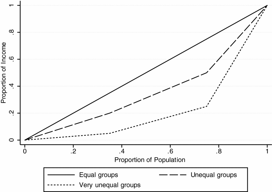
Figure 1 illustrates BGI using the Lorenz curve for three hypothetical societies, each divided into three groups—group 1, group 2, and group 3—with 35, 40, and 25 members, respectively. Each society has 100 units of income to distribute among these groups. In a completely equal society, group 1 will receive 35 units of wealth, group 2 will receive 40 units of wealth, and group 3 will receive 25 units of wealth. The Lorenz curve will be a straight line because the group occupying the “bottom” 35% of the income distribution controls 35% of the income, the groups occupying the “bottom” 75% of the income distribution control 75% of the income, and so on. This case is depicted by the solid black line. BGI in this case is 0.

FIGURE 1.

Graphical Illustration of BGI

In an unequal society, the wealthiest group will control more income per person than the poorest group. The long dashed line draws the Lorenz curve if group 1 controls only 20% of the income, group 2 controls only 30% of the income, and group 3 controls 50% of the income. In this case, the group occupying the bottom 35% of the income distribution control only 20% of the income, and the two groups occupying the bottom 75% of the income distribution control only 50% of the income. The BGI in this case is 0.275. The short dashed line depicts the Lorenz curve in an even more unequal society in which group 1 controls just 5% of the income, group 2 controls 20%, and group 3 controls 75%. In this case, the bottom 75% of the income distribution controls only 25% of the society's income and BGI is 0.55.

Like the Gini, BGI ranges from 0 to 1. It takes on its minimum value of 0 when the average incomes of all groups in society are the same, and it takes on its maximum value of 1 when one infinitely small group controls all the income in society. Put another way, for any level of ELF, BGI will be 0 if all groups have the same mean income. Holding ELF constant, BGI is increasing in the income differences between groups. The effect of income differences across groups on BGI will be largest when ELF is largest. BGI will take its largest values when there are many equally sized groups (as with ELF) and when the income differences between the groups are large. Between-group inequality, then, can be viewed as an extension of the ELF that allows income differences between groups to vary. Conversely, ELF can be viewed as a restriction on between-group inequality that holds differences between all groups constant at 1.

MEASURING BETWEEN-GROUP INEQUALITY USING EXISTING SURVEYS

The main empirical challenge in analyzing the effects of between-group economic differences is constructing national-level measures of BGI for a large set of countries. A number of different scholars have constructed ELF measures (Alesina et al. Reference Alesina, Devleeschauwer, Easterly, Kurlat and Wacziarg2003; Fearon Reference Fearon2003), and Fearon (Reference Fearon2003) and Desmet, Ortuo, and Weber (Reference Desmet, Ortuño and Weber2009) have created measures of cultural fractionalization for almost all the countries in the world. But existing cross-national data sets do not include measures of between-group inequality, in part because BGI requires information on the economic well-being of groups that is not readily available from secondary sources. The construction of BGI for a particular country requires information on both the size of ethnic groups within the country and the economic well-being of these groups. This section describes how existing cross-national surveys—the Afrobarometer, the WVS, and the CSES—can be used to create BGI measures, and provides evidence regarding the validity and biases of the resulting measures.

The Afrobarometer, WVS, and CSES surveys all contain instruments that make it possible to identify the “ethnicity” of respondents. However, ethnic categories often nest inside broader categories, and as Posner (Reference Posner2004) demonstrates, choices about which groups to include can have a significant impact on the conclusions one draws about the relationship between group diversity and outcomes. A decision rule is therefore necessary to decide which groups are most relevant in a particular country. In this article, we follow the identification of groups made by Fearon (Reference Fearon2003) as closely as possible because we believe that Fearon's work is the most careful and theoretically motivated classification of groups that has been completed to date. His seven criteria emphasize groups that are understood as “descent groups” and that are locally viewed as socially or politically consequential. Depending on the country, Fearon's identification of groups may be based on race (e.g., the US), language (e.g., Belgium), religion (e.g. France), tribe (e.g., many African countries), or even some combination of these factors. He draws on a range of secondary sources to identify the size of each group for the vast majority of countries in the world, and the resulting data set provides both a guide for the creation of the BGI measure and a benchmark against which to judge it.

In classifying survey respondents into groups, we mirror as closely as possible the groups used by Fearon. In the US, for example, Fearon identifies four ethnic groups: whites, blacks, Hispanics, and Asians. Variable x051 in the WVS has seven categories: white, black, Hispanic, other, central Asian, south Asian, and east Asian. We convert this sevenfold variable to the Fearon groups by recoding the three Asian groups to “Asian” and dropping “Other.” It is not always possible to place all respondents into one of the Fearon groups. In France, for example, he identifies the groups as French, Muslim, and Bretons. Using the CSES, we cannot identify the Bretons, but we can identify the French and Muslims.

To determine whether the Fearon groups are sufficiently well identified by a survey to merit the inclusion of the survey in the data set, we have employed a 15% rule. The rule works as follows. For each survey, we calculate the percentage of the population (per Fearon's data) that we cannot assign to any of Fearon's groups, and we retain the survey if this number is less than 15%. In France, for example, the only “missing group”—that is, the only group that Fearon identifies but that we cannot identify in the French surveys—is the Bretons, who (according to Fearon) represent 4.6% of the French population. We keep the French survey because 4.6% is less than our 15% threshold. In Israel, in contrast, Fearon distinguishes Arabs (15% of the population) and Palestinians (22%). Neither the CSES nor the WVS has an ethnic category for Palestinians, and because they represent more than 15% of the population, we exclude these Israeli surveys. The following analysis also presents results that follow a 5% rule, which obviously sets a higher standard for including countries in the data set.

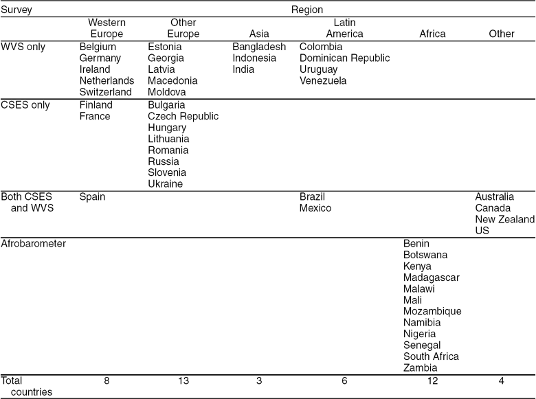
We are interested in which types of ethnic diversity are associated with governance problems in countries that are at least minimally democratic. We focus on democracies because dictators have little incentive to provide public goods regardless of the ethnic diversity of their countries (Olson Reference Olson1993; Sen Reference Sen1999), and the effect of ELF on governance has been found to differ in democratic and authoritarian countries (Collier Reference Collier2000). We therefore consider only countries that have a Polity 2 score of 1 or higher. Some countries have more than one survey, and when this occurs, we average BGI scores across the surveys for that country. The resulting 46 countries included in the analysis are listed in Table 1. The Afrobarometer surveys are from waves 2 and 3 (2002–2006), the CSES surveys are from all three waves (1996–2003), and the WVS surveys are from wave 4 (1996 and 1999). The sample includes democracies from all regions of the world, although we underrepresent Asia and especially Latin America in so far as these regions have a higher proportion of the world's democracies than their representation in this data set suggests.

TABLE 1.

Countries in Study

CSES, Comparative Study of Electoral Systems; WVS, World Values Survey.

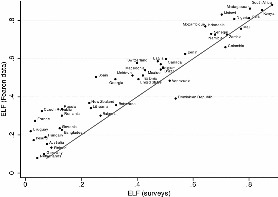
How well do the survey data reflect the composition of groups? It is straightforward to answer this by constructing a measure of ELF from the survey data and comparing this to the ELF scores from Fearon (Reference Fearon2003). If one accepts the Fearon data as a good benchmark approximation of the true level of ethnic fractionalization, then one should have confidence in the survey-based measures only if the correlation between the survey data ELF and the Fearon ELF is strong. Figure 2 plots this relationship for the 46 countries. The survey-based ELF, which takes the average value within countries when there is more than one survey in a country, is obviously very closely related to the Fearon ELF. The Fearon-based measures typically take higher values, particularly at low levels of fractionalization, but the overall correlation is an impressive 0.96 [which is higher than the correlation between Fearon's measures of ELF and Alesina et al.'s (Reference Alesina, Devleeschauwer, Easterly, Kurlat and Wacziarg2003) measures of ELF].

FIGURE 2.

Comparing Ethnolinguistic Fractionalizations (ELFs): Fearon Data versus Survey Data

The next challenge is measuring group economic well-being. Ideally, one would construct the BGI measure using fine-grained, individual-level income or consumption data, aggregated by group. There currently do not exist a large number of multinational surveys that contain this type of data with appropriate information about group identity, but the Afrobarometer, WVS, and CSES surveys contain coarse measures of each respondents' economic well-being that can be used to evaluate the relative well-being of different groups. Even coarse data on group income differences provides information that can be used to measure BGI.

Each survey measures respondents' income or consumption using a different metric. For example, the WVS survey asks the respondent to answer the following question:

The respondent is given a country-specific scale, typically with 8 to 10 categories, created to be meaningful within each country. Each CSES country survey asks a similar question to the WVS, but the CSES reports only the income quintiles of the respondents.

The Afrobarometer survey, like most surveys in developing parts of the world, does not have an income variable. For many individuals in these countries, such a question would be meaningless because the individuals have little or no cash income. Instead, the common strategy in such surveys is to ask respondents questions about their access to things crucial to their basic needs. For the Afrobarometer, each survey asks respondents a number of questions of the following type:

In addition to asking about food, the survey asks about water, medical care, cooking fuel, and cash income. Each variable is coded on a five-point scale (from 0 to 4) according to how often the respondent has gone without the item. The sum of the responses from these five questions can be used to create an economic well-being metric that ranges from 0 (maximal unmet needs) to 20 (no unmet needs). This index is obviously most useful in distinguishing differences among the least well-off, masking differences that exist among the more well-to-do.

These “income” variables, along with the group identity variables, make it possible to calculate BGI for each survey. In cases where we have multiple surveys for a given country, we average across surveys to create a score for each country.Footnote ⁶ Validating this BGI measure is more difficult than validating the survey data on group composition because no benchmark data exist. However, because the measures of income are coarse and thus do not fully characterize the income distribution, it is important to assess the validity of the measures and to be aware of biases they may possess.

We can gain some sense of the validity of the income measures by examining whether they reflect income disparities in the handful of cases where the nature of inequality between ethnic groups is widely acknowledged. It is reassuring to note that in the survey, whites are richer than Mulattos who are richer than blacks in Brazil; Bulgarians are richer than Turks in Bulgaria; the Flemish are wealthier than the French in Belgium; whites are wealthier than Mestizos and blacks in the Dominican Republic; Muslims are poorer than the “French” in France; and whites are richer than blacks and Hispanics in the US. In the African countries, where the income measures are most limited in that they only distinguish between differences among the poor, the data still capture the fact that whites and people of mixed race background are wealthier than other ethnic groups in Namibia, the Ibo and Yoruba are richer than the Hausa in Nigeria, and whites, coloureds, and Asians are richer than blacks in South Africa. Thus, in these cases where the income relationships between groups are known, there is considerable face validity in the way that the data rank the relative incomes of groups.

The problem, of course, is that data on between-group economic differences has not been previously collected on a large scale, so little is known about the economic differences between many other groups. To gain further insight into the validity of the BGI measures, we turned, where possible, to household income surveys with very fine-grained measures of income. Few surveys exist that identify income by the ethnic groups in our data set, but we identified household surveys that could be used to construct measures of the income or expenditures of the relevant ethnic groups for nine countries in our data set: Brazil, Bulgaria, Canada, Estonia, Finland, Germany, the US, South Africa, and Zambia.Footnote ⁷ Although this is too few surveys to use in studying the relationship between BGI and public goods provision, these surveys allow an examination of the extent to which the survey measures used here differ from those constructed from finer-grained income data.

The correlation between the measures using our surveys and the measures from the household surveys is 0.68. But South Africa is a huge outlier, with a BGI in the fine-grained data that is three times higher than the next country, Brazil. If we exclude South Africa, the correlation between BGI from our surveys and BGI from the fine-grained expenditure surveys is an impressive 0.85. South Africa, of course, has a unique history of apartheid, which concentrated enormous wealth in the hands of whites. Our survey does not capture the magnitude of the inequality in South Africa because the Afrobarometer only measures the fact that virtually no whites in South Africa are poor. However, even so, our data rank South Africa as having the third highest level of BGI in our data set, after the Dominican Republic and Brazil, suggesting that our data do a good job of ranking countries in terms of BGI.

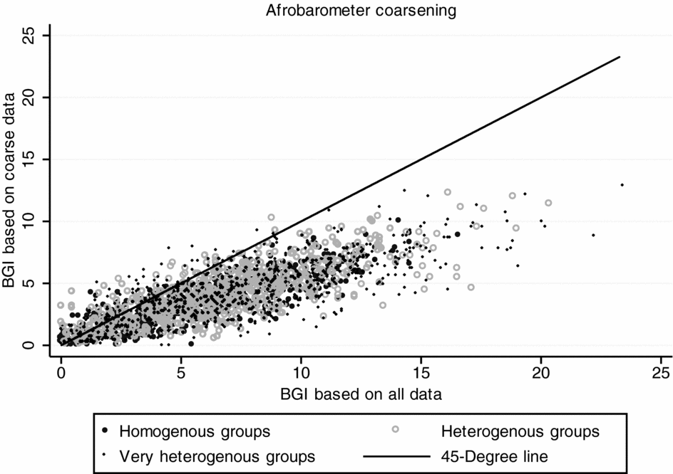
As a final strategy for exploring how the Afrobarometer's focus on income differences among the poor affect measures of BGI, we conducted simulations. As described in more detail in Appendix 1, the simulated data set contains thousands of societies made up of individuals whose exact income was known. To replicate the Afrobarometer coarsening technique, we assigned all people above a fixed poverty line in the simulated income data to the richest category and then divided the poor into different income levels based on their absolute level of deprivation. We then constructed measures of BGI for each society based on the “true” income variable and the “coarsened” income variable.

Figure 3 plots the true BGI (based on the fine-grained income distribution) against the coarsened income data (where income differences exist only at low income levels, as in the Afrobarometer). The dark xs represent societies where there are minimal income differences within ethnic groups (homogenous groups), the solid gray dots represent societies where there are some income differences within ethnic groups (heterogenous groups), and the open gray circles represent societies where there are large income differences within ethnic groups (very heterogenous groups). Figure 3 also depicts the 45-degree line, making it easy to identify whether “coarsening” leads to overestimates (points above the line) or underestimates (points below the line) of the true BGI. Not surprisingly, we can see that for any assumption about group income heterogeneity and for any of the three coarsening techniques, on average, the coarsened metrics underestimate the true level of between-group inequality. But we also find that the correlation between the true BGI and the BGI based on the coarsened data is very strong, ranging from 0.76 (when groups are most heterogenous) to 0.87 (when groups are most homogenous).

FIGURE 3.

Simulating the Effect of Afrobarometer Data on Estimates of Between-Group Inequality (BGI)

Thus, the simulations reinforce what we found in the previous data: despite the fact that the Afrobarometer suppresses information about income differences among the nonpoor, it provides measures of BGI that are highly correlated with finer measures of BGI. Furthermore, the Afrobarometer measures are biased in the “right” direction to the extent that they systematically underestimate the true BGI. This should make it more difficult to find differential results of ELF and BGI on public goods provision.

COMPARING ETHNOLINGUISTIC FRACTIONALIZATION, CULTURAL FRACTIONALIZATION, AND BETWEEN-GROUP INEQUALITY

ELF, CF, and BGI measure theoretically distinct concepts. But are the three measures also empirically distinct? Are the countries with the greatest linguistic differences between ethnic groups different from the countries with the greatest economic differences between groups?

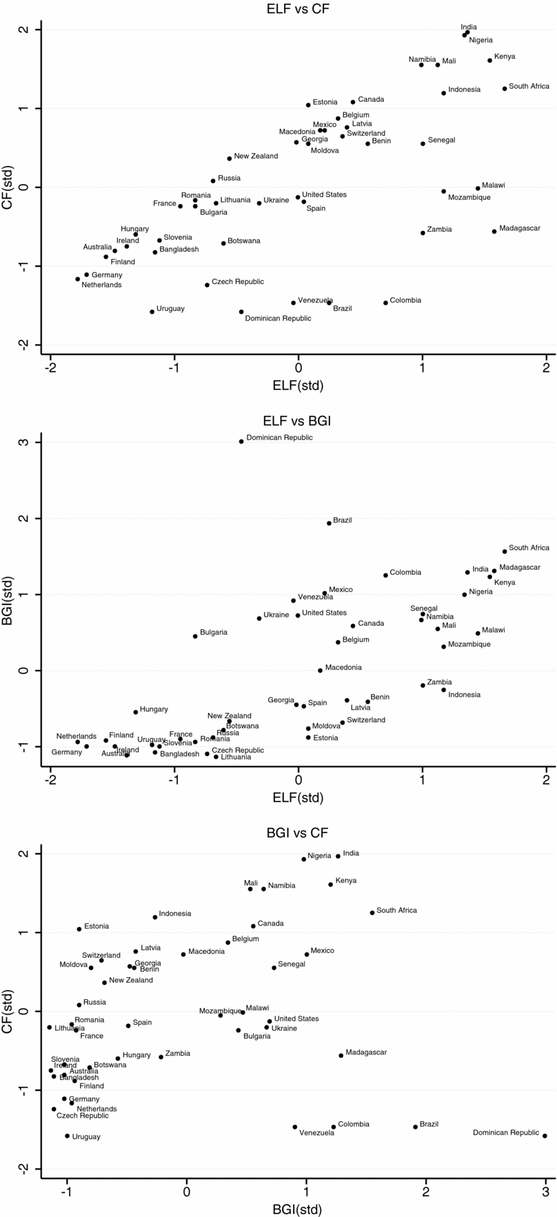
Figure 4 depicts the relationships between the three measures of ethnic diversity, with each of the measures standarized to have a mean of 0 and a standard deviation of 1. First, consider the relationship between CF and ELF, which is also discussed in Fearon (Reference Fearon2003). For his full set of countries, he found that the two measures are highly correlated (r = 0.79), with the largest differences occurring in sub-Saharan Africa and Latin America. In our subset of 46 countries, the correlation between ELF and CF is 0.64, somewhat lower than in Fearon's full data set. The top panel in Figure 4 shows that the correlation between the two variables is relatively strong throughout the range of ELF, but definitely weakens as ELF grows. A number of countries with high ELF—particularly those in Latin America—have groups that use similar languages. The countries whose diversity rankings are most affected by the switch from ELF to CF are listed in Table 2. Colombia ranks 13th in ELF and only 43rd in CF because the various ethnic groups in Colombia all speak Spanish. Madagascar is the second most diverse country in the data using ELF. But all groups in Madagascar speak Malagasy or a closely related language, so Madagascar's CF score ranks only 30th in the data. Russia and Estonia, in contrast, move in the other direction, each increasing 13 places in the country rankings when one switches from ELF to CF. This is because the main language groups in these countries are from different language families.

FIGURE 4.

Ethnolinguistic Fractionalization (ELF), Cultural Fractionalization (CF), and Between-Group Inequality (BGI) in 46 Countries

TABLE 2.

Countries Whose Diversity Rankings Change Most When Switching from ELF to CF

CF, cultural fractionalization; ELF, ethnolinguistic fractionalization.

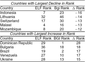
Second, consider the relationship between ELF and BGI, which is depicted in the middle panel of Figure 4. As with the previous comparison, there is a strong correlation between the two variables (r = 0.62), but for many countries, their relative ranking depends substantially on which measure is used. Among the low BGI countries, there is a wide range of ELF scores, and among the high ELF scores, there is a wide range of BGI scores. Table 3 lists the countries whose diversity rankings are most affected by the change from ELF to BGI. Indonesia is the country that declines the most: it is ranked 7th using ELF but only 23rd using BGI. The Dominican Republic moves sharply in the opposite direction: it is ranked only 29th using ELF but has the highest BGI in the data set.

TABLE 3.

Countries Whose Diversity Rankings Change Most When Switching from ELF to BGI

BGI, between-group inequality; ELF, ethnolinguistic fractionalization.

The bottom panel in Figure 4 examines the relationship between CF and BGI. The correlation between these two variables (r = 0.17) is quite weak. As is clear in Figure 4, a number of countries, particularly in Latin America, have very high levels of between-group inequality but low levels of language difference. Furthermore, there are a number of countries, particularly in eastern and central Europe, where language differences are large, but between-group economic differences are relatively small.

The analysis therefore demonstrates that the three diversity measures, although related, are clearly distinct. The relative rankings of the countries change, at times dramatically, across the different measures. Incorporating information about cultural fractionalization or the economic well-being of groups therefore alters how we understand the relative ethnic diversity of countries.

GROUP DIFFERENCES AND PUBLIC GOODS PROVISION

Although the three measures differ, do the differences matter for understanding the relationship between diversity and public goods provision? Does one of the measures have a stronger relationship with public goods provision than the others, suggesting that it may be the more important factor driving the relationship between ethnic diversity and poor governance outcomes? This section presents results from a series of regression models that analyze the relationship between the measures of diversity and public goods provision.

The models in this section treat a country as the unit of analysis. As noted previously, the survey data used to construct the BGI measures are from the 1996 to 2006 time period. When multiple surveys exist for a given country, we average across the surveys, minimizing measurement error that may be associated with particular surveys. We also average the World Bank's World Development Indicators (WDIs) used to measure public goods over the 1996 to 2006 period, which is important given that the WDIs are often missing in particular years. Because ELF and CF are constant over time, the strategy of using a country as a unit of analysis also facilitates comparison of the correlations between the various measures of diversity and public goods provision. However, it is difficult to settle questions about whether diversity affects public goods or public goods affect diversity in this framework. The next section therefore estimates models that treat each survey as the unit of analysis in an effort to gain additional insight regarding causation.

To measure public goods provision, we rely on ten variables in the World Bank's WDIs, each related to government-provided public goods, such as public health, education, public infrastructure, and the government's taxing capacity. There are a larger number of candidate variables in the WDI data set, but many have large numbers of missing values. We averaged the country values for each variable for the period 1996–2006, and then retained only those variables such that (1) none of the 46 countries had more than 3 missing, and (2) no variable was missing for more than 7 of the 46 countries. The resulting ten variables used in the analysis, with the number of missing countries in brackets, are as follows:

• • Expenditure per student, primary (% of GDP per capita) [7] (WDI variable name = SE.XPD. PRIM.PC.ZS)

• • Public spending on education, total (% of GDP) [1] (SE.XPD.TOTL.GD.ZS)

• • Immunization, measles (% of children aged 12–23 months) [0] (SH.IMM.MEAS)

• • Immunization, DPT (% of children aged 12–23 months) [0] (SH.IMM.IDPT)

• • Improved sanitation facilities (% of population with access) [7] (SH.STA.ACSN)

• • Improved water source (% of population with access) [6] (SH.H2O.SAFE.ZS)

• • Roads, paved (% of total roads) [0] (IS.ROD. PAVE.ZS)

• • Procedures to enforce a contract (number) [0] (IC.LGL.PROC)

• • Tax revenue (% of GDP) [4] (GC.TAX.TOTL. GD.ZS)

• • Telephone lines (number per 100 people) [0] (IT.MLT.MAIN.P2)

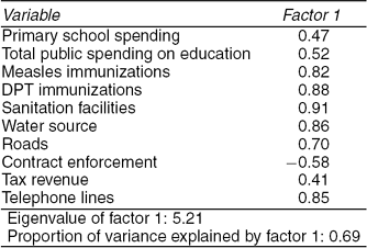
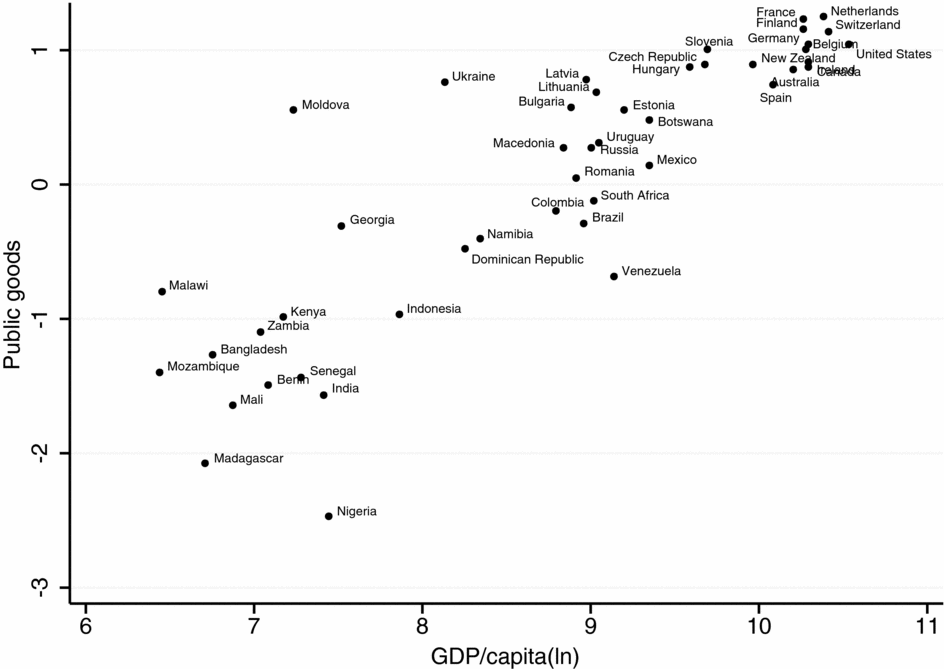
Each variable alone is a noisy predictor of the overall level of public goods provision in a country, susceptible to measurement error that is likely idiosyncratic to particular countries. Therefore, rather than choosing one or more specific variables for analysis, we use the information from all ten variables to create a single measure of the overall level of public goods provision. To this end, we conduct a factor analysis on all ten variables. We first impute the values of the missing variables, where missing values on one of the ten variables are imputed as a function of the other nine.Footnote ⁸ We then use Bartlett scoring on the first dimension of the factor analysis to create the dependent variable, which we call Public Goods. The results for the first factor in this factor analysis are shown in Table 4. All ten of the variables load strongly on the first factor. The variables with the strongest relationship to the underlying factor, and which therefore receive the greatest weight in the construction of the public goods variable, are immunizations, sanitation, water, and telephone lines, all with factor loadings greater than 0.8. Two variables have a loading that is less than 0.5—Tax Revenue and Primary School Spending—but each variable still has a relatively strong relationship with the underlying factor. The first factor has an eigenvalue of 5.21 and explains 69% of the variance in these ten variables. Figure 5 plots Public Goods against the log of GDP per capita (measured in purchasing power parity). The two variables are obviously strongly correlated, but at any level of economic development, and in particular at lower levels of development, there exists variation in the level of public goods.

TABLE 4.

Factor Analysis of Public Goods Variables

FIGURE 5.

Public Goods Provision and National Wealth

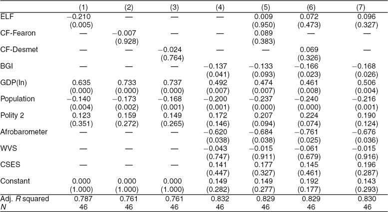
We estimate OLS models with robust standard errors using Public Goods as the dependent variable. The models include several controls. One is the level of economic development [GDP/capita (ln), measured using purchasing power parity], which is known to have a very strong relationship with the level of public goods provision. Scholars have also emphasized the importance of democracy for public goods provision (e.g., Lake and Baum Reference Lake and Baum2001), and although we focus on countries that are in some sense democratic (achieving Polity 2 scores of greater than or equal to 1), there is considerable variation within our data set regarding the development of democratic institutions and practices. We therefore include Polity 2 as a control for the level of democratic institutionalization. It is also important to take into account the population of a country. If there are economies of scale, then public goods provision may be largest in the most populous countries. But if the most populous countries present the most challenges to governance, public goods provision may be negatively correlated with population. The correlation matrix for all right-hand-side variables is given in Appendix 2. For models that include the BGI measure based on the surveys, there are four indicator variables that identify the survey(s) used to create an observation. These dummy variables indicate whether a measure was constructed from the Afrobarometer, the WVS (equals 1 if country uses only WVS), the CSES (equals 1 if country uses only CSES), or the WVS/CSES (equals 1 if country uses both WVS and CSES, which is the omitted category). The indicators are included because the surveys use different measures of “income,” which likely results in differences in the degree to which they underestimate the true level of between-group differences. In the regression models, we standardize each continuous right-hand-side variable to have a mean of 0 and a standard deviation of 1. This makes it straightforward to compare the size of the effects of the different variables. The parentheses in the tables provide the p values for the estimated coefficients.

In Table 5, models 1 to 4 include the controls and one of the measures of diversity. Model 1 includes ELF. Consistent with previous research, the coefficient for ELF is in the expected negative direction and is very precisely estimated. Model 2 uses Fearon's cultural fractionalization measure of diversity. The coefficient is in the expected negative direction but is very small and estimated with considerable error. Model 3 uses the Desmet, Ortuño, and Weber measure of cultural fractionalization instead of Fearon's measure. The coefficient has the wrong sign and is also estimated with considerable error. Finally, in model 4, the coefficient for BGI is negative and very precisely estimated. In models including only one measure of ethnic diversity, then, ELF and BGI have a clear relationship to public goods provision, but cultural differences do not.

TABLE 5.

Group Differences and Public Goods Provision I

Notes: P values based on robust standard errors are in parentheses. BGI, between-group inequality; CF, cultural fractionalization; CSES, Comparative Study of Electoral Systems; ELF, ethnolinguistic fractionalization; GDP, gross domestic product; WVS, World Values Survey.

Next we examine the results when we include measures of each form of diversity in the same model. Model 5 uses the Fearon measure of cultural fractionalization, and model 6 uses the Desmet, Ortuño, and Weber measure. In both models, the coefficient for cultural fractionalization is very imprecisely estimated and has the wrong sign. The models also show that when BGI and ELF are included in the same model, the relationship between ELF and Public Goods disappears. The ELF coefficient now has the wrong sign and is estimated with large error, whereas the coefficient from BGI remains negatively and rather precisely estimated, especially in model 6.

We have estimated a wide range of additional models, and the results for cultural fractionalization are consistently estimated with very large error and often have the wrong sign. Because there is no empirical support for including this variable and it is strongly correlated with ELF, model 7 presents results when only BGI and ELF are included (along with the controls). ELF is positive, although it is estimated with considerable error, and the coefficient for BGI remains negative and precisely estimated. These results from Table 5 therefore suggest the possibility that in previous research claiming a correlation between ELF and public goods provision, the relationship was actually being driven by between-group economic differences.

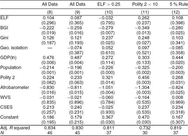
How robust is this result? We first address this question by exploring the possibility of spurious correlation due to omitted variables. Scholars have argued that inequality may affect collective behavior and public goods provision. Many scholars have hypothesized that inequality is negatively associated with social cohesion (Boix and Posner Reference Boix and Posner1998; Knack and Keefer Reference Knack and Keefer1997; Uslaner Reference Uslaner2002, Reference Uslaner2008). Khwaja (Reference Khwaja2009) finds that inequality makes it more difficult for communities to create infrastructure projects, and Bardhan (Reference Bardhan2000) and Dayton-Johnson (Reference Dayton-Johnson2000) find that inequality in landholdings negatively affects the collective management of water resources. One might therefore worry that between-group inequality is simply a proxy for inequality more generally. We test this possibility using a measure of Gini from Solt (Reference Solt2009), who uses the Luxembourg Income Study to enhance the data from the United Nations University's World Income Inequality Database. The coefficient for Gini in model 8 is positive, but it is measured with considerable error. The result for BGI is robust to the inclusion of the Gini variable.

Next consider the geographic segregation of groups. Geographic segregation could make it more difficult to provide groups in remote areas with public goods. To the extent that geographic isolation could be correlated with between-group differences, we can have more confidence that the relationship between between-group differences and public goods is not spurious if we control for the level of group geographic segregation. We control for geographic segregation using a measure of Geographic Isolation derived from work by scholars of residential segregation. This measure is described in Appendix 3. It takes higher values when geographic segregation is greater, and interestingly, it has a negative correlation with BGI (r = −0.64). Geographic Isolation should have a negative coefficient if it makes public goods provision more difficult.

Model 9 adds Geographic Isolation to model 8. The coefficient on the variable has the expected negative sign but is estimated with substantial error. The inclusion of this variable, however, does not affect the conclusions about ELF and BGI. ELF remains insignificant, whereas BGI is negative and precisely estimated. The relationship between BGI and PG found in the previous regressions should not therefore be attributed to a spurious correlation between either variable and the geographic segregation of groups.

We then test the robustness of the BGI result by reestimating model 9 using different subsets of the data. The data set contains a number of very homogenous countries, many of which are quite rich and have high levels of public goods provision. Model 10 therefore examines whether the results are robust when we include only highly heterogenous countries, with an ELF greater than 0.25. The result for BGI is essentially unchanged when the data are restricted to this subsample of the 37 most heterogenous countries. The ELF coefficient remains estimated with extremely large error. Similarly, the previous analysis includes a number of countries that are very well-established democracies, where problems of ethnic diversity are often held to be relatively small. Model 11 therefore focuses on the less established democracies by eliminating the 16 countries that have a Polity 2 score of 10. The results indicate that when the strongest democracies are excluded, the effect of BGI remains very precisely estimated and in fact has the largest absolute magnitude of any model in Tables 5 and 6.

TABLE 6.

Group Differences and Public Goods Provision II

Notes: P values based on robust standard errors in parentheses. BGI, between-group inequality; CSES, Comparative Study of Electoral Systems; ELF, ethnolinguistic fractionalization; GDP, gross domestic product; WVS, World Values Survey.

Finally, some may be concerned that the “15%” rule for replicating the Fearon groups is too lax, resulting in the inclusion of countries that have relatively large groups that are not represented in the surveys. To address this concern, we implemented a 5% rule for the retention of countries. That is, we aggregated the total population of the groups for which we could not assign the respondents. If this constituted less than 5% of the population, then we retained the survey. Otherwise, we eliminated the survey from the data set. The change in the retention rule eliminates eight countries and ensures that any group that Fearon identifies that does not exist in our surveys is very small. The results from the 5% rule, presented in model 12, are consistent with those in the other models. The coefficient for BGI remains negative, quite large in absolute value, and precisely measured.

Across a range of models, then, standard measures of ethnic fractionalization and cultural fractionalization do not have a robust correlation with public goods provision. The same holds for the level of inequality. Between-group inequality, in contrast, does have a negative relationship with public goods provision, one that is robust to a wide range of model specifications and decisions about which countries to include in the analysis. Furthermore, the effect is large. Bearing in mind that we standardized the right-hand-side variables to facilitate comparisons, simply inspecting the regression output indicates that the estimated coefficient for BGI is very large relative to other variables. For example, in model 9, the model containing all controls and the full data set, in absolute value, the BGI coefficient is more than double the estimated coefficient for ELF or Gini, and roughly the same size as the estimated coefficient for Polity 2.

DOES BETWEEN-GROUP INEQUALITY LEAD TO LOWER PUBLIC GOODS PROVISION?

The previous analysis establishes that when we control for between-group inequality, standard measures of ELF and cultural fractionalization are not correlated with public goods provision, whereas between-group inequality does have a robust correlation with public goods. Existing theoretical arguments focus on the possibility that between-group economic differences make policy agreement more difficult and invite discrimination by powerful groups against less powerful ones, lowering public goods provision. But between-group inequality is also likely the result of policy decisions regarding public goods. If clean water or paved roads or education expenditures, for example, can be targeted at specific groups, then such targeting could lead to between-group economic differences. And if public goods tend to help the least well-off, then public goods should diminish between-group inequality whenever there is a correlation between income and group.

This section presents several additional models exploring whether BGI causes lower public goods provision (as opposed to simply being correlated with public goods). The data do not permit us to address this issue definitively, largely because the time series is very short, there are too few observations on BGI, and there is too much missing data on public goods provision. But by taking advantage of the temporal component of the data, we can provide some evidence that between-group economic differences lead to lower levels of public goods.

The first step is to redefine “income” in the Afrobarometer surveys so as to reduce the possibility that the measure of economic well-being in Africa is endogenous to the measure of public goods provision. Recall that the consumption-based measure from the Afrobarometer surveys includes five components, and two of these are related to access to public services (medical care and clean water). The measure of public goods similarly includes measures of health care (immunizations) and water (percent of population with access). It is therefore plausible that public goods provision is directly affecting the measure of BGI in the African countries included in the analysis. In the results presented previously, we include the information about access to health care and clean water to create as fine-grained a measure as possible about the economic well-being of Afrobarometer respondents. This is particularly important given the skew of the “needs” variables toward the “rich” in the Afrobarometer surveys. But given the endogeneity concern, it is important to reestimate the models using a measure of BGI in Africa that does not incorporate information on individuals' access to public services; this measure of BGI has been constructed based only on individuals' reported access to food, cooking oil, and cash income.

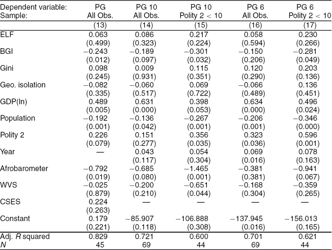
Model 12 in Table 7 presents the results when model 9 is reestimated using the recalculated measures of BGI in Africa. The results are very consistent with those in model 9: BGI has a negative coefficient that is precisely measured. ELF continues to be insignificant (and has the wrong sign). There is no significant relationship between inequality and public goods. The results from the previous models were therefore not driven by the potential endogeneity between the BGI measure in Africa and the measure of public goods.

TABLE 7.

Exploring the Causal Effect of BGI on Public Goods

Notes: P values based on robust standard errors are in parentheses. BGI, between-group inequality; CSES, Comparative Study of Electoral Systems; ELF, ethnolinguistic fractionalization; GDP, gross domestic product; WVS, World Values Survey.

The next step is to use this recoded data (that excludes the endogenous items in the Afrobarometer) in models that treat each survey as an observation. The strategy is simple. If we measure BGI at time t and public goods using data subsequent to time t, it is more difficult to argue that public goods are influencing the level of between-group inequality. As noted previously, this approach is not without problems, particularly because the measure of public goods suffers missing data issues. But using surveys as the unit of analysis provides an opportunity to examine whether BGI has a causal impact on public goods.

To measure the dependent variable, if the survey is taken at time t, we take the average value for each component of the public goods measure in times t through t + 3 and then use the four-year averages to create the public goods measure as before.Footnote ⁹ The missing data problems in this approach are substantially more severe than they are in the aggregate approach because there are a number of four-year periods for which there are no data for particular variables. The contract enforcement variable, for example, is present only toward the end of the period covered by our data, and thus is missing for 53% of the survey-specific observations. Sanitation, water, and roads are each missing for at least 37 % of observations. Given the missing data issues, we present results for two different versions of the public goods variable. The first, which we call PG10, uses all variables, whereas the second, PG6, uses only the six variables for which less than 25% of observations are missing. These are the two immunization variables, the two education variables, tax revenues, and telephones.

Models 14 to 17 in Table 7 use the survey-specific data to estimate the same specification as model 9, except that we now include a variable, Year (the year of the survey), to capture positive time trends that often exist in the provision of public goods, particularly in developing parts of the word.Footnote ¹⁰ Model 14 uses PG10 as the dependent variable and uses all available observations. The coefficient on BGI is negative, with a p value of .097. The coefficient on ELF, in contrast, has the wrong sign and is measured with considerable error. Model 15 reestimates the same model as 14, but using only countries with Polity 2 scores of less than 10. The estimated coefficient for BGI increases substantially in size and is much more precisely estimated (p = 0.032) in comparison with model 15. Models 16 and 17 use PG6 as the dependent variable. In model 16 (all data), BGI has the expected negative coefficient but has a standard error that is larger than that found in other models. ELF continues to have the wrong sign and to be measured with considerable error. Model 17 includes only countries with Polity 2 less than 10, and the BGI coefficient is negative, substantively large and precisely estimated. If we assume, then, that public goods in the future cannot affect between-group inequality in the past, then these results provide evidence that between-group inequality causes lower levels of public goods. This effect of BGI on public goods is particularly evident when we omit the most politically developed countries from the sample.