3.1. General description of quadruplets

We define a quadruplet as four wave vectors $\boldsymbol {k}_1$ , $\boldsymbol {k}_2$ , $\boldsymbol {k}_3$ , $\boldsymbol {k}_4$ satisfying the resonant conditions (2.2) and (2.3). These quadruplets constitute a five-dimensional manifold. We perform a normalisation of quadruplets with respect to direction and scale to introduce a three-dimensional manifold of normalised quadruplets.

The kinetic equation (2.1) is isotropic, so the properties of a quadruplet must not depend on its orientation. We fix the orientation by fixing the direction of the $\boldsymbol {k}_{1+2}$ vector. All the angles will be measured with respect to this vector.

The coefficient $T$ with dispersion relation (2.4) permits the scaling

(3.1) \begin{equation} T(a\boldsymbol {k}_1,a\boldsymbol {k}_2,a\boldsymbol {k}_3,a\boldsymbol {k}_4) = a^3\, T(\boldsymbol {k}_1,\boldsymbol {k}_2,\boldsymbol {k}_3,\boldsymbol {k}_4). \end{equation}

We will use the ‘base vector’ $\boldsymbol {k}_B=\boldsymbol {k}_{1+2}/2$ as the scale base. All the vectors will be normalised to $k_B$ , while $T$ will be normalised to $k_B^3$ . This $T$ normalisation is convenient everywhere except in the region where $k_{1+2}$ is small (‘angular quadruplets’; see § 4.4). In that region, we have to use $(k_1k_2k_3k_4)^{3/4}$ as the normalisation for $T$ .

The difference between the two normalisations does not affect the general behaviour of $T$ . The notable exceptions are the quadruplets with small $k_{1+2}$ mentioned above, and the long–short interactions (see § 4.3).

It is well known (Longuet-Higgins Reference Longuet-Higgins1976) that for equal vectors $\boldsymbol {k}_1=\boldsymbol {k}_2=\boldsymbol {k}_3=\boldsymbol {k}_4 =\boldsymbol {k}_B$ , we have

(3.2) \begin{equation} k_B^{-3}\, T(\boldsymbol {k},\boldsymbol {k},\boldsymbol {k},\boldsymbol {k}) =2. \end{equation}

An appropriate choice of normalisation allows us to find that for opposite vectors $\boldsymbol {k}_1=-\boldsymbol {k}_2$ , $\boldsymbol {k}_3=-\boldsymbol {k}_4$ , we have $k_1=k_2=k_3=k_4=k$ and

(3.3) \begin{equation} k^{-3}\, T(\boldsymbol {k},{-\boldsymbol {k}},\boldsymbol {k},{-\boldsymbol {k}}) = -2. \end{equation}

We will suggest below that these values are local extrema. Numerical calculations show that the normalised $T$ is globally bounded by these values:

(3.4) \begin{equation} -2 \leqslant \frac {T(\boldsymbol {k}_1,\boldsymbol {k}_2,\boldsymbol {k}_3,\boldsymbol {k}_4)}{(k_1k_2k_3k_4)^{3/4}} \leqslant 2. \end{equation}

The $T$ coefficient is invariant with respect to several permutations of vectors. These are the $\boldsymbol {k}_1 \leftrightarrow \boldsymbol {k}_2$ permutation, the $\boldsymbol {k}_3 \leftrightarrow \boldsymbol {k}_4$ permutation, and also the double permutation $\boldsymbol {k}_1 \leftrightarrow \boldsymbol {k}_3,\ \boldsymbol {k}_2 \leftrightarrow \boldsymbol {k}_4$ . This symmetry allows us to deal with only part of the quadruplet space. In particular, it is convenient to set

(3.5) \begin{equation} k_1 \leqslant k_2, \quad k_3 \leqslant k_4. \end{equation}

Some notable special cases may be mentioned. First, there is the case of pairwise coinciding vectors $\boldsymbol {k}_1=\boldsymbol {k}_3$ , $\boldsymbol {k}_2=\boldsymbol {k}_4$ studied in Lavrova (Reference Lavrova1983). Such quadruplets do not transfer energy, for geometrical reasons, but have non-trivial $T$ . Then there is the one-dimensional case when all the vectors are collinear, studied in Dyachenko et al. (Reference Dyachenko, Kachulin and Zakharov2017). This case has two variants. First, the collinear vectors may be coinciding pairwise. Alternatively, three vectors may be of the same direction, with the fouth one of opposite direction. It is shown in Dyachenko & Zakharov (Reference Dyachenko and Zakharov1994) and Dyachenko et al. (Reference Dyachenko, Kachulin and Zakharov2017) that for such quadruplets, $T=0$ . Therefore, there is no four-wave interaction in the one-dimensional case. Nevertheless, this case is interesting for the study of nearly-collinear wave packets.

3.2. Coordinates

Fixing the normalisation and the direction leaves us with three coordinates of a quadruplet to deal with. Let us discuss the choice of these coordinates.

The coordinate that is convenient and significant in the classification of quadruplets is the ‘modulus’ $s$ defined as

(3.6) \begin{equation} \omega _1+\omega _2=\omega _3+\omega _4=2s\,\sqrt {gk_B}. \end{equation}

The modulus $s$ is bounded by

(3.7) \begin{equation} \frac {\sqrt {2}}{2}\lt s\lt +\infty. \end{equation}

For the long–short interactions, $s= ({\sqrt {2}}/{2})(1+r)$ , $r\ll 1$ .

A significant case is $s=1$ ; see § 4.1.

Large values of $s$ correspond to the interactions between the vectors of close lengths but different directions.

The conditions

(3.8) \begin{align} & \omega _1+\omega _2=2s\sqrt {gk_B}, \nonumber \\ & \boldsymbol {k}_1+\boldsymbol {k}_2=2\boldsymbol {k}_B \end{align}

define a curve at the $\boldsymbol{k}$ plane for any $s$ (figure 1 shows some such curves). Any two points of this curve define a quadruplet: $\boldsymbol {k}_1$ and $\boldsymbol {k}_2$ are defined by one point, and $\boldsymbol {k}_3$ and $\boldsymbol {k}_4$ by the other one. The quadruplet symmetry allows us to choose both these points on the left-hand side of the curve.

Figure 1.

The ‘Phllips eight’ curve (thick line) and some other lines of $s=\textrm {const}$ (thin lines). Also shown is the DIA quadruplet ( $s=1$ , $\lambda _1=0.25$ , $\lambda _3=0$ ). $k_x$ and $k_y$ are the x and y coordinates of $k_1$  and  $k_3$ vectors.

The Zakharov equation covers not only the resonant surface but the area outside it as well. The non-resonant quadruplets there may be described with two separate moduli defined by $(\omega _1+\omega _2)/2$ and $(\omega _3+\omega _4)/2$ (both equal to $s$ on the resonant surface). Some approximations introduced here should be valid in the vicinity of the resonant surface, but these constructions are beyond the scope of the present paper. See Dyachenko et al. (Reference Dyachenko, Kachulin and Zakharov2017) for some simplifications of $T$ for the Zakharov equation.

We will use the parameter $s$ for the classification of quadruplets. The remaining two coordinates are less significant. The simplest choice for them would be the angles $\theta _1$ and $\theta _3$ (which are measured between two smaller vectors and $\boldsymbol {k}_B$ ). Another option is to use $\lambda _1$ and $\lambda _3$ (the numbering correspond to the numbering of wave vectors) such that

(3.9) \begin{eqnarray} \omega _1=(1-\lambda _1)\sqrt {gk_B}, \quad \omega _2=(1+\lambda _1)\sqrt {gk_B}, \nonumber \\ \omega _3=(1-\lambda _3)\sqrt {gk_B}, \quad \omega _4=(1+\lambda _3)\sqrt {gk_B}. \end{eqnarray}

The advantage of $\lambda _{1,3}$ coordinates lies in the fact that all the parameters of quadruplet vectors may be derived from them using elementary functions only. Their drawback is the singularity at the horizontal axis. They are also double-valued.

Finally, we note that other parametrisations of the resonance manifold are possible. Moreover, the base vector may be chosen in other ways (e.g. one may use $\boldsymbol {k}_{1-3}$ ). We try to minimise the explicit use of our coordinates. Therefore, all the final formulae are written here in terms of the $\boldsymbol{k}$ vectors and without the use of the normalisation.

4.1. DIA-like quadruplets

One of the first methods of simplification of the four-wave interaction pattern was suggested by Phillips (Reference Phillips1960). He considered the resonance between a main wave taken twice, and two other waves. This corresponds to $\boldsymbol {k}_3=\boldsymbol {k}_4$ . In this case, the endpoints of the $\boldsymbol {k}_1$ and $\boldsymbol {k}_2$ vectors lie on the curve that is known as the ‘Phillips eight’ (figure 1).

The DIA method proposed by Hasselmann et al. (Reference Hasselmann, Hasselmann, Allender and Barnett1985) uses only one symmetric pair of quadruplets. Historically, this was the first (though severely simplified) representation of (2.1) in quadruplet form. The DIA quadruplet is

(4.1) \begin{equation} \omega _1=(1-\lambda )\omega _B, \quad \omega _2=(1+\lambda )\omega _B, \quad \omega _3=\omega _4=\omega _B, \end{equation}

with $\lambda =0.25$ . This quadruplet is shown in figure 1.

The Phillips eight curve is indeed of great importance. Its central part is a geometric singularity. The large area around the singularity is populated by similar kinds of vector pairs. Vector pairs in the vicinity of the singularity ( $\boldsymbol {k}_1\approx \boldsymbol {k}_2\approx \boldsymbol {1}$ ) are composed of two nearly equal vectors. If one substitutes such a pair by the two equal vectors (represented by the centre of the curve), then the resulting changes of the two vectors are small and anticollinear. The changes in $N_i$ in (2.1) resulting from such a substitution compensate each other to first order due to the anticollinearity. This means that all the points near the centre may be substituted by the central point without a significant loss of precision. Such a substitution requires a shift of the other point of the quadruplet, but this shift is small for the points that are away from the centre because the curves of constant $s$ converge there. This is why the DIA quadruplet may adequately represent a whole family of similar quadruplets. This explains the viability of the DIA method.

While the DIA-like quadruplets account for a significant part of the wave interactions, they do not represent the entire variety of interactions. Notably missing from the DIA method are interactions between waves of different angles (which play a role in the transfer of energy from the main peak of wind waves to the waves travelling sideways or against the wind). Also, the DIA method seriously limits the long–short waves interaction range.

The above considerations justify a dedicated study of the Phillips curve. In terms of the coordinates introduced above, this curve is defined by $s=1$ .

We introduce a class of DIA-like quadruplets defined by (4.1) with arbitrary $\lambda$ . (For $s=1$ we have $-1/2 \leqslant \lambda \leqslant 1/2$ ). The coefficient $T$ for this case may be calculated explicitly as

(4.2) \begin{eqnarray} T_{\boldsymbol {k}_1\boldsymbol {k}_2\boldsymbol {k}_B\boldsymbol {k}_B} = \frac {k_B^3}{2\sqrt {1-\lambda ^2}} \, \big (2+\lambda ^2\big )^2 \,\big (1-4\lambda ^2\big ) \left (1- \frac {2}{3} \left (\vert \lambda \vert \sqrt {6+\lambda ^2} + \lambda ^2\right ) \right ). \end{eqnarray}

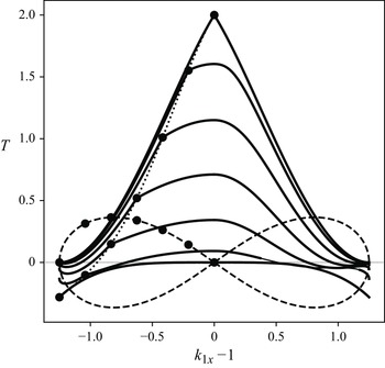
This function is shown on figure 2 as the top line.

In particular, for the DIA quadruplet with $\lambda =0.25$ ,

(4.3) \begin{equation} T_{\textit {DIA}}\approx 0.903\, k_B^3. \end{equation}

At the sides of the Phillips curve, (4.2) is small. Let us take the $\theta _1$ such that ${\unicode[Arial]{x03C0}} -\theta _1\ll 1$ (which corresponds to the left-hand side of the curve). Then $\lambda \approx ({1}/{2})- {({\unicode[Arial]{x03C0}} -\theta _1)^2}/{36}$ and

(4.4) \begin{equation} T_{\boldsymbol {k}_1\boldsymbol {k}_2\boldsymbol {k}_B\boldsymbol {k}_B}\approx \frac {\sqrt 3}{80}\, k_B^3 \, ({\unicode[Arial]{x03C0}} -\theta _1)^4. \end{equation}

This implies that the interaction between the side and central part of the curve is small. The dynamically significant part of the curve is the central ‘cross’. It may be defined approximately by $\vert \lambda \vert \lt 0.42$ . (We take here the $\lambda$ for $\theta _1={\unicode[Arial]{x03C0}} /2$ , for this value $T\approx 0.14$ .)

Now we explore arbitrary $\lambda _1$ and $\lambda _3$ (while still keeping $s=1$ ). Figure 2 shows a set of graphs of $T/k_B^3$ for different $\lambda _3$ values. For clarity, the graph also shows the Phillips curve (dashed line). The abscissa axis represents ${k}_{1x}-1$ ( ${k}_{1x}$ being the $x$ -component of $\boldsymbol {k}_{1}$ ). This coordinate is used for both the Phillips curve and the $T$ graphs; the corresponding $\lambda _1$ may be determined from ${k}_{1x}$ as ${k}_{1x}-1=-2(\lambda _1+\lambda _1^3)$ . The set of fixed $\lambda _3$ points for the graphs is shown as dots on the Phillips curve. The points with $\lambda _1=\lambda _3$ are marked on the graphs; these points constitute the $T_{\boldsymbol {k}_1\boldsymbol {k}_2\boldsymbol {k}_1\boldsymbol {k}_2}$ graph that is also shown (dotted line).

Figure 2.

The $T/k_B^3$ coefficient graphs for the Phillips curve quadruplets. The quadruplets are specified by two points at the curve. One of them is fixed for each of the $T$ curves (and chosen at the left-hand side of the Phillips curve), while the other moves at the top part of the ‘eight’ curve. The fixed point is marked both on the Phillips curve and in the corresponding $T$ graph (at the same abscissa). The abscissa of the moving point is used as the $T$ graph independent coordinate. The marks on the $T$ graphs correspond to the quadruplets with coinciding vector pairs, which allows us to draw the graph of $T_{\boldsymbol {k}_1\boldsymbol {k}_2\boldsymbol {k}_1\boldsymbol {k}_2}$ through these marks (dotted line).

We also present a two-dimensional graph of $T$ in figure 3. Obviously, this graph cannot represent the whole three-dimensional space of quadruplets, but it is useful for understanding of the general behaviour of $T$ . The $xy$ plane of this graph represents the points that define the $\boldsymbol {k}_1$ and $\boldsymbol {k}_2$ vectors; corresponding lines of $s$ are also shown. The figure shows the $T$ graph for the quadruplet defined by these $\boldsymbol {k}_1$ , $\boldsymbol {k}_2$ , while the $\boldsymbol {k}_3$ , $\boldsymbol {k}_4$ are chosen as follows. For $s\lt 1$ , the point representing $\boldsymbol {k}_3$ and $\boldsymbol {k}_4$ is chosen at the $x$ axis such that $\boldsymbol {k}_3$ and $\boldsymbol {k}_B$ are collinear. For $s\gt 1$ , such a point does not exist, and we use a central point such that $\boldsymbol {k}_{3y}=1$ . Such a choice yields $\boldsymbol {k}_3$ and $\boldsymbol {k}_4$ close to $\boldsymbol {k}_B$ whenever possible. The vertical axis represents $T/(k_1k_2k_3k_4)^{3/4}$ . Such a normalisation is chosen for the graph to be finite.

The graph in figure 3 shows that $T$ is large at the central zone. It crosses zero somewhere at a larger $s$ , then continues to decrease up to the value $-2$ (beyond the graph boundary). Also note that at the ends of the Phillips curve, $T$ is small (it is exactly zero at the adjacent part of the abscissa axis).

Figure 3.

A two-dimensional cross-section of the $T/(k_1k_2k_3k_4)^{3/4}$ graph. To make this cross-section from the three-dimensional quadruplet space, one of the quadruplet points was chosen at the $x$ axis for $s\lt 1$ , or at the $y$ axis for $s\gt 1$ . The other point is used as the independent coordinate.

4.2. Central quadruplets

The central part of the quadruplet manifold (where all four vectors are nearly equal) is of particular interest. While most of the quadruplets describe non-local interactions, these central quadruplets are an example of the local interaction. They were studied before in Longuet-Higgins (Reference Longuet-Higgins1976) and Dungey & Hui (Reference Dungey and Hui1979), where the expansion at the central point of the Phillips curve was used to construct an approximate diffusion-like method of calculation of the energy transfer. This approach results in the Dysthe equation, which is a generalisation of the nonlinear Schrödinger equation (Dysthe Reference Dysthe1979).

The central quadruplets provide an interesting insight into the mechanism of energy transfer. Nevertheless, their transfer rate is weakened for geometrical reasons (the nearly equal vectors result in smaller difference in (2.1)). The DIA-like quadruplets described above still benefit from the large $T$ and from the considerable width of the central area, but they also connect different parts of the spectrum (the length ratio between ‘long’ and ‘short’ vectors in the DIA quadruplet (4.1) is $2.78$ ). For these reasons, they provide a large part of the energy transfer.

The central area includes many quadruplets and has a large (actually, maximum) $T$ . In this domain,

(4.5) \begin{equation} \boldsymbol {k}_1=\boldsymbol {k}_B-\boldsymbol{\varkappa }_1, \quad \boldsymbol {k}_2=\boldsymbol {k}_B + \boldsymbol {\varkappa }_1, \quad \boldsymbol {k}_3=\boldsymbol {k}_B-\boldsymbol {\varkappa }_3, \quad \boldsymbol {k}_4=\boldsymbol {k}_B+\boldsymbol {\varkappa }_3, \end{equation}

where $\varkappa _1$ and $\varkappa _3$ are small parameters:

(4.6) \begin{equation} \varkappa _1 \ll k_B,\quad \varkappa _3 \ll k_B. \end{equation}

Then $T$ is

(4.7) \begin{align} T=2k_B^3 & \left \{ 1-\frac {(\varkappa _{1x}-\varkappa _{3x})^2} {2\,\sqrt {(\varkappa _{1x}-\varkappa _{3x})^2 +(\varkappa _{1y}-\varkappa _{3y})^2}}\right .\nonumber \\&\left .\quad{} -\frac {(\varkappa _{1x}+\varkappa _{3x})^2} {2\,\sqrt {(\varkappa _{1x}+\varkappa _{3x})^2 +(\varkappa _{1y}+\varkappa _{3y})^2}} +o(\varkappa ) \right \}. \end{align}

One can see from (4.7) that the first-order correction to $T$ is negative except for $\varkappa _{1x}=\varkappa _{3x}=0$ . One more order is required to deal with the latter case. The second-order correction is also negative, which proves that $T_{\boldsymbol {kkkk}}$ is indeed the maximum. The details of the calculation are given in Appendix A.

We may restrict ourselves to the $s=1$ curve. In this area, the curve is defined by

(4.8) \begin{equation} \varkappa _{1y}=\pm \frac {\sqrt 2}{2}\varkappa _{1x}, \quad \varkappa _{3y}=\pm \frac {\sqrt 2}{2}\varkappa _{3x}. \end{equation}

A quadruplet is defined by two points on this curve. If they are on the same branch of (4.8), then the expression (4.7) can be simplified:

(4.9) \begin{equation} T=2k_B^3 \left \{ 1 - \frac {2\sqrt 6}{3} \lambda _1 + o(\lambda ) \right \}. \end{equation}

Here, we have set $\vert \lambda _1\vert \gt \vert \lambda _3\vert$ . The result is independent of $\lambda _3$ .

4.3. Long–short interactions

Equation (2.1) is non-local. It includes interactions between waves with different $\boldsymbol {k}$ that are not nesesserily close to each other. The most drastic case of non-locality is the long–short interaction. While most quadruplets are composed of vectors of comparable lengths, long–short interaction quadruplets may include vectors with an arbitrarily large length ratio.

We show that the interaction coefficient for the long–short interactions is surprisingly small. In the calculation of the coefficient, the two higher orders of the expansion turn out to be zero. The underlying reason for this is still unknown. This smallness significantly reduces the non-locality of the kinetic equation, and increases the role of energy and wavenumber cascading.

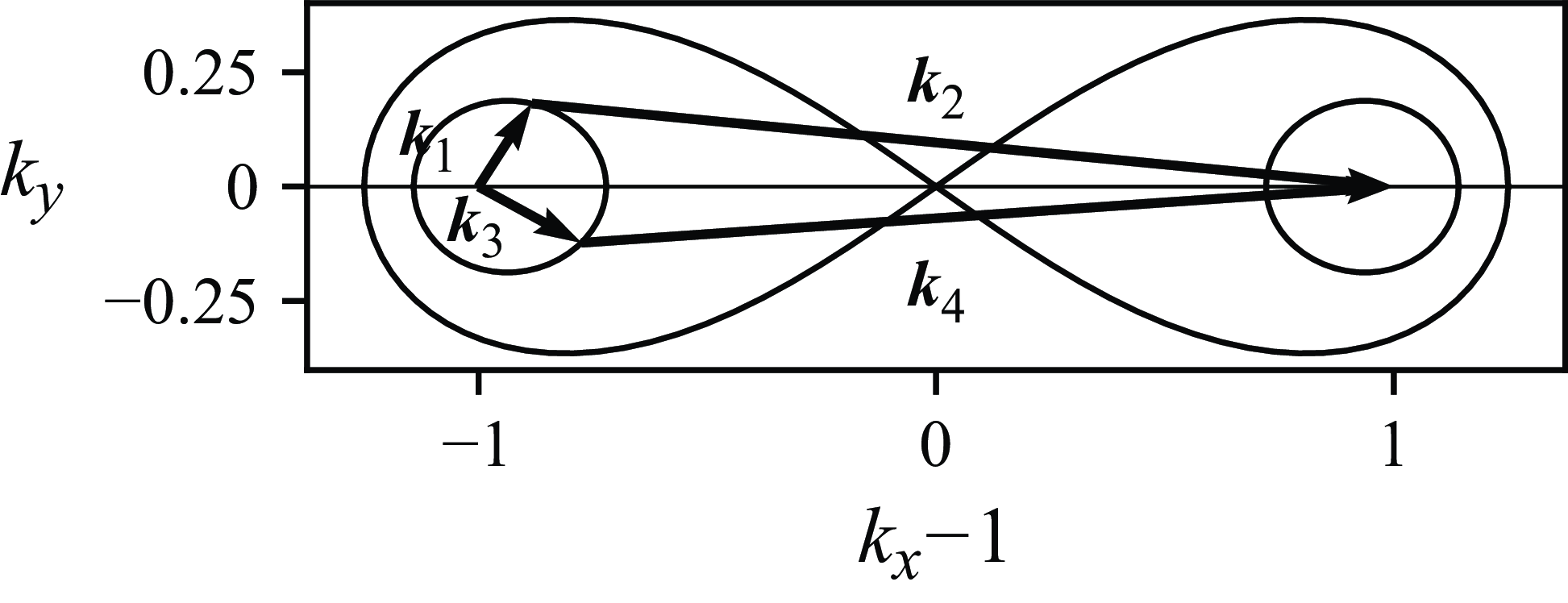
Figure 4 shows a typical long–short interaction quadruplet. Such quadruplets include two nearly equal long vectors $\boldsymbol {k}_2$ , $\boldsymbol {k}_4$ , and two short vectors $\boldsymbol {k}_1$ , $\boldsymbol {k}_3$ that are approximately equal in length but have arbitrary directions.

Figure 4.

An example of a long–short quadruplet. Also shown are the Phillips curve and the $s=\textrm {const}$ curve for this quadruplet.

We will use a small parameter $r$ defined by

(4.10) \begin{equation} \omega _1+\omega _2=\omega _3+\omega _4=(1+r)\sqrt {k_{1+2}}. \end{equation}

We have

(4.11) \begin{eqnarray} k_2\approx k_4 \approx k_{1+2},\quad k_1\approx k_3 \approx r^2 k_{1+2}. \end{eqnarray}

The other two independent variables are $\theta _1$ (the angle between $\boldsymbol {k}_1$ and $\boldsymbol {k}_{1+2}$ ) and $\theta _3$ (the angle between $\boldsymbol {k}_3$ and $\boldsymbol {k}_{1+2}$ ).

Extremely complicated calculations (included here as Appendix B) yield the following result:

(4.12) \begin{equation} T = \frac {r^4 k_{1+2}^3}{2} \, (\cos \theta _1+\cos \theta _3) \, (1+\cos (\theta _1-\theta _3)) + o\big(r^4\big). \end{equation}

The expansion of $T$ by the small parameter $r$ has a very surprising property: two higher orders of the expansion are zeros.

It may be that to some extent, the long–short interaction quadruplets border the quadruplets at the vicinity of the Phillips curve.

4.4. Angular quadruplets

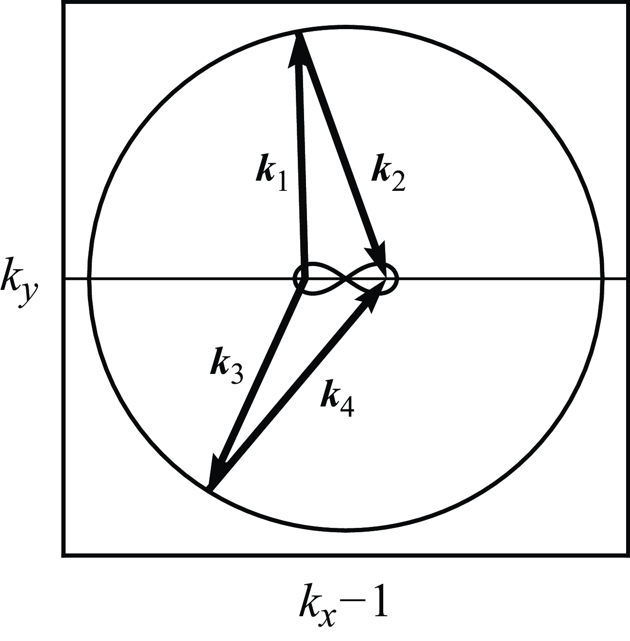
A significant and distinct class of the quadruplets includes ones describing the interaction between the waves of close frequencies travelling in different directions. Their characteristic property is a small $\boldsymbol {k}_{1+2}$ vector. We propose to call them ‘angular quadruplets’. An example of such a quadruplet is shown in figure 5.

Figure 5.

An example of an angular quadruplet. Also shown are the Phillips curve and the $s=\textrm {const}$ curve for this quadruplet.

For these quadruplets, we have

(4.13) \begin{equation} \boldsymbol {k}_2\approx - \boldsymbol {k}_1, \quad \boldsymbol {k}_4\approx - \boldsymbol {k}_3, \end{equation}

which results in

(4.14) \begin{equation} k_1\approx k_2\approx k_3\approx k_4 \gg k_{1+2}. \end{equation}

Let $k$ be the length of (approximately equal) vectors of an angular quadruplet. Then $T$ becomes

(4.15) \begin{equation} T \approx -\frac {k^3}{2} \left (3+\cos ^2\theta _{1-3} \right ), \end{equation}

where $\theta _{1-3}$ is the angle between $\boldsymbol {k}_1$ and $\boldsymbol {k}_3$ or between $\boldsymbol {k}_2$ and $\boldsymbol {k}_4$ .

If $\theta _{1-3}=0$ , then the minimum value of $T$ is achieved. This may be demonstrated by calculating the partial derivatives at this point. Equation (4.15) shows that the derivative by $\theta _{1-3}$ is zero. For the other two coordinates, we may choose the $\boldsymbol {k}_{1+2}$ vector. One can see from the symmetry of (2.5) that the derivatives with respect to both its components are zero.

The angular quadruplets are located further apart from the Phillips curve. The quadruplets in between are different both from DIA-like and angular ones.

4.5. Quadruplets variety

We have described different classes of quadruplets and the behaviour of $T$ for these classes. Let us summarise what parts of the quadruplet manifold were studied.

The long–short interactions (characterised by $s-\sqrt 2/2 \ll 1$ ) directly border the DIA-like quadruplets. In fact, the side part of the Phillips curve may be considered as the long–short interactions as it has smaller vectors of size approximately $1/4$ , and larger ones of size approximately $9/4$ .

The DIA-like quadruplets occupy the vicinity of the Phiilps curve ( $s\approx 1$ ). This include the large area near the geometric singularity at the centre of the curve.

The quadruplets that are further outside the Phillips curve ( $s\gt 1$ ) were not covered in the present paper. They occupy an intermediate place between the DIA-like quadruplets and the ‘angular’ ones, and may have properties similar to both of these kinds. The $T$ coefficient crosses zero in this area; nevertheless, many of these quadruplets having non-zero $T$ are significant.

The outside part of the $\boldsymbol {k}$ plane is occupied by the ‘angular’ quadruplets ( $s\ll 1$ ). They have a simple asymptotic described above.