1 Introduction
Despite significant progress over the past decades, taming flow instabilities and turbulence remains an area of fundamental investigation (Kim & Bewley Reference Kim and Bewley2007; Brunton & Noack Reference Brunton and Noack2015; Sipp & Schmid Reference Sipp and Schmid2016). The potential impact of flow control is however tremendous: drag reduction, lift increase, mixing enhancement, noise reduction, lean combustion to name a few industrial applications. Control strategies fall into two broad categories: active or passive, depending whether energy is expended to drive an actuator or not. Actuation may be used in an open-loop framework, in order to drive the system away from its natural state by exciting its nonlinearities. For this strategy to be effective, a large power input may be required. On the other hand, closing the loop has a direct impact on the intrinsic dynamics of a linear system, hence the actuation amplitude may be significantly reduced (Cattafesta III et al. Reference Cattafesta, Song, Williams, Rowley and Alvi2008). However, uncertainties in the form of noise or modelling errors may cause instabilities or performance loss of the closed loop, which in turn render the approach ineffective.
1.1 On the relevance of linear methods for closed-loop control of nonlinear flows
In the particular case of fluid flows, modelling issues arise from the dimensionality of the system and the strong nonlinearity of the governing equations. Dimensionality reduction is often achieved by projecting the dynamics onto a set of well-chosen modal structures, and well-established techniques exist to systematically find such bases, e.g. global modes, proper orthogonal decomposition (POD) modes, balanced modes (BPOD), dynamic modes (DMD), etc. (Bagheri, Brandt & Henningson Reference Bagheri, Brandt and Henningson2009; Barbagallo, Sipp & Schmid Reference Barbagallo, Sipp and Schmid2009; Semeraro et al. Reference Semeraro, Bagheri, Brandt and Henningson2011; Rowley & Dawson Reference Rowley and Dawson2017 for a comprehensive review). Alternatively, if system identification is used to derive a reduced-order model (ROM) directly from input–output data (Cattafesta et al. Reference Cattafesta, Shukla, Garg and Ross1999; Kegerise, Cattafesta III & Ha Reference Kegerise, Cattafesta and Ha2002; Illingworth, Morgans & Rowley Reference Illingworth, Morgans and Rowley2011; Dahan, Morgans & Lardeau Reference Dahan, Morgans and Lardeau2012; Hervé et al. Reference Hervé, Sipp, Schmid and Samuelides2012; Dalla Longa, Morgans & Dahan Reference Dalla Longa, Morgans and Dahan2017), the resulting models will typically be of manageable dimension. Suitable ROMs for closed-loop control may also be obtained by gradually increasing the spatial discretization from a coarse mesh (Jones et al. Reference Jones, Heins, Kerrigan, Morrison and Sharma2015).
Nonlinearity, on the other hand, remains a major issue as the standard control tool set relies extensively on the hypothesis of a linear time-invariant (LTI) plant. Early studies therefore focussed on the linear dynamics of small perturbations around a base flow, i.e. a fixed point of the Navier–Stokes equations. Techniques were successfully developed to suppress intrinsic instabilities or prevent extrinsic noise amplification: oscillator flows may be controlled by damping their unstable modes using a feedback controller, while amplifier flows may be controlled by rejecting incoming perturbations using an upstream sensor (see Sipp & Schmid Reference Sipp and Schmid2016, for a review). In some cases, the designed controllers may also be robust to nonlinearities; for instance if the Reynolds number is weakly supercritical, in the case of an unstable base flow (Flinois & Morgans Reference Flinois and Morgans2016), or if incoming perturbations are large, in the case of a stable base flow (Hervé et al. Reference Hervé, Sipp, Schmid and Samuelides2012). However, for strong enough nonlinearity, linearization about the base flow becomes irrelevant and control fails (Schmid & Sipp Reference Schmid and Sipp2016).
In the case of self-sustained oscillations, which are of interest in this paper, there are indeed (at least) two distinct dynamical equilibria: the steady fixed point, and the unsteady attractor. In the uncontrolled flow, the fixed point is linearly unstable and the attractor lies at a finite distance from it in phase space. In this situation, the goal of a controller is not just to locally stabilize the base flow but to ensure that any initial condition on the attractor is within the basin of attraction of the base flow. If the attractor is not too far away from the base flow, then a robust LTI controller based on some mean LTI model may suffice (Li & Morgans Reference Li and Morgans2016). But again, for strong enough nonlinearity, modelling the plant as a single LTI operator may be too crude an approximation, and even robust control methods based on it may fail.
Significant efforts were therefore directed towards nonlinear reduced-order modelling. Physics-based nonlinear ROMs usually rely on Galerkin projection of the full Navier–Stokes equations (as opposed to the linearized version around the fixed point), most often using POD modes. However, such models typically require fine tuning and calibration because of instabilities stemming from the structure of the expansion and its truncation (Noack et al. Reference Noack, Schlegel, Morzyński and Tadmor2011). While designing nonlinear ROMs is a challenge of fundamental interest by itself, it is however not immediately clear that their enhanced fidelity can be made profitable for closed-loop control applications. Indeed, optimal control based on such ROMs represent an enormous computational load (Bergmann, Cordier & Brancher Reference Bergmann, Cordier and Brancher2005) for realistic application in experiments. Besides, adjoint looping only yields a specific control command optimized over a given time horizon for a given initial condition of the system.
An alternative to nonlinear Galerkin models is nonlinear identification from input–output data (second-order Volterra and bilinear filters, Pillarisetti & Cattafesta III (Reference Pillarisetti and Cattafesta2001); NARX, Dandois, Garnier & Pamart (Reference Dandois, Garnier and Pamart2013); NARMAX, Semeraro et al. (Reference Semeraro, Lusseyran, Pastur and Jordan2017), cluster-based ROM, Kaiser et al. (Reference Kaiser, Noack, Cordier, Spohn, Segond, Abel, Daviller, Östh, Krajnović and Niven2014); SINDy, Loiseau & Brunton (Reference Loiseau and Brunton2018), etc.) but the resulting models are usually not used for feedback control. Artificial neural networks have been trained to learn complex input–output relations (Lee et al. Reference Lee, Kim, Babcock and Goodman1997; Efe et al. Reference Efe, Debiasi, Yan, Özbay and Samimy2005), but a controller design simply based on inversion of the neural net does not bring any improvement compared to existing LTI controllers. Another novel approach to tackle nonlinearity is machine-learning control (Duriez et al. Reference Duriez, Parezanovic, Laurentie, Fourment, Delville, Bonnet, Cordier, Noack, Segond and Abel2014; Gautier et al. Reference Gautier, Aider, Duriez, Noack, Segond and Abel2015): a model-free approach which seeks a nonlinear control law through trial and error. Although promising, the approach is not amenable to physical analysis and interpretation, which may hinder further improvements in case of failure.
Systematic methods for deriving nonlinear control laws, i.e. relations from outputs to inputs applicable at any time, although more useful, are in fact rarely implemented in practice. It has only been done so far with analytically tractable ‘mean-field’ ROMs of order 4 at most, for flows dominated by at most two frequencies, i.e. a single one for the unforced flow plus one for the actuator (King et al. Reference King, Seibold, Lehmann, Noack, Morzyński and Tadmor2005; Aleksić et al. Reference Aleksić, Luchtenburg, King, Noack and Pfeifer2010; Luchtenburg et al. Reference Luchtenburg, Aleksić, Schlegel, Noack, King, Tadmor, Günther and Thiele2010; Aleksić-Roessner et al. Reference Aleksić-Roessner, King, Lehmann, Tadmor and Morzyński2014). Furthermore, although superior in some cases (Aleksić-Roessner et al. Reference Aleksić-Roessner, King, Lehmann, Tadmor and Morzyński2014), nonlinear controllers do not systematically show obvious improvements compared to their linear counterparts. More complex nonlinear ROMs are in fact generally linearized about their fixed point, in order to design traditional LTI controllers (Samimy et al. Reference Samimy, Debiasi, Caraballo, Serrani, Yuan, Little and Myatt2007; Nagarajan, Cordier & Airiau Reference Nagarajan, Cordier and Airiau2013). While this procedure removes a lot of information from the initial model, the physical meaning of the fixed point is unclear, as it is not directly related to either the mean flow or the base flow of the true system.
Finally, passivity-based methods are suited to finite-amplitude perturbations of the base flow and, therefore, hold great promise for the problem of nonlinear flow control (Sharma Reference Sharma2009; Sharma et al. Reference Sharma, Morrison, McKeon, Limebeer, Koberg and Sherwin2011; Heins, Jones & Sharma Reference Heins, Jones and Sharma2016). The key idea is to see the fluid flow as a Lur’e system (Khalil Reference Khalil2002), i.e. the nonlinearity of the governing equations is a feedback forcing to the linearized dynamics about the base flow (more details will be given in §§ 2.1 and 2.2). Since nonlinearity in the Navier–Stokes equations arises from conservative processes, it cannot contribute to the energy growth of external perturbations; i.e. it is passive. Therefore, one is only concerned with energy growth arising from the linear processes. Methods are available to design LTI controllers preventing linear energy growth altogether (Sharma et al. Reference Sharma, Morrison, McKeon, Limebeer, Koberg and Sherwin2011) or, if impossible, at least minimizing it (Heins et al. Reference Heins, Jones and Sharma2016), but these methods have only been applied to linearly stable flows so far.
This brief overview of available nonlinear flow control methods explains why, to date, the vast majority of successful studies rely on LTI models and controllers, even though the underlying plant is nonlinear.
1.2 A physics-based linear framework relevant to nonlinear flows: mean-flow perturbation analysis
In the following, we distinguish the base flow, defined as a fixed point of the Navier–Stokes equations, and the mean flow, which is the temporal average of a fully developed flow.
1.2.1 Modal analysis
Since Hammond & Redekopp (Reference Hammond and Redekopp1997), many authors have considered mean-flow stability analysis as a means to retrieve both the nonlinear oscillation frequency of globally unstable base flows and the coherent structure oscillating at that fundamental frequency. Most studies were concerned with wake flows (Hammond & Redekopp Reference Hammond and Redekopp1997; Pier Reference Pier2002; Barkley Reference Barkley2006; Mittal Reference Mittal2007; Sipp & Lebedev Reference Sipp and Lebedev2007; Leontini, Thompson & Hourigan Reference Leontini, Thompson and Hourigan2010; Meliga, Pujals & Serre Reference Meliga, Pujals and Serre2012; Camarri, Fallenius & Fransson Reference Camarri, Fallenius and Fransson2013; Mettot, Sipp & Bézard Reference Mettot, Sipp and Bézard2014b ; Mantič-Lugo & Gallaire Reference Mantič-Lugo and Gallaire2016; Carini et al. Reference Carini, Airiau, Debien, Léon and Pralits2017), where mean-flow distortion leads to a significant reduction of the length of the recirculation region behind the solid body, compared to the base flow. Other configurations have been considered as well, among which open-cavity flow (Sipp & Lebedev Reference Sipp and Lebedev2007; Meliga Reference Meliga2017), gas turbine fuel injectors (Juniper Reference Juniper2012) and thermosolutal convection (Turton, Tuckerman & Barkley Reference Turton, Tuckerman and Barkley2015). We note that in resonant flows, coherent structures are rigorously described by Koopman modes, and the oscillation frequencies correspond to Koopman eigenfrequencies (Arbabi & Mezić Reference Arbabi and Mezić2017).
1.2.2 Resolvent analysis
For globally stable flows, the temporal instability framework does not properly account for the noise amplifier dynamics. In parallel flows, spatial stability analysis may be used to predict the response to localized harmonic forcing. In non-parallel flows, the resolvent operator may be used instead to predict the linear response of the flow to any spatially distributed forcing. Connections between local and global analyses obviously exist for weakly non-parallel flows. Global spatial modes obtained from solving parabolized stability equations may approximate optimal response modes obtained by singular value decomposition (SVD) of the resolvent operator (Beneddine et al. Reference Beneddine, Sipp, Arnault, Dandois and Lesshafft2016). But the resolvent operator is more than a mere extension of spatial stability analysis to the global framework. It fully describes the input–output behaviour of the flow. In particular, SVD of the resolvent operator not only yields a set of optimal response modes approximated by spatial instability modes, it also provides the associated set of optimal forcing modes and optimal gains giving insight into the receptivity mechanisms at play in the flow.
When high-amplitude noise excites the nonlinearities in amplifier flows, coherent motions seem to extract energy from the mean flow, rather than the base flow (Butler & Farrell Reference Butler and Farrell1993; Chomaz Reference Chomaz2005; Del Álamo & Jimenez Reference Del Álamo and Jimenez2006; Cossu, Pujals & Depardon Reference Cossu, Pujals and Depardon2009; Pujals et al. Reference Pujals, García-Villalba, Cossu and Depardon2009). And just like mean-flow temporal modes capture the dominant coherent structures of resonator flows, mean-flow spatial modes or optimal response modes (often called resolvent modes) seem to capture the dominant coherent structures of amplifier flows. In that context, the coherent structures may be rigorously defined as spectral POD modes (Gudmundsson & Colonius Reference Gudmundsson and Colonius2011; Beneddine et al. Reference Beneddine, Sipp, Arnault, Dandois and Lesshafft2016; Towne, Schmidt & Colonius Reference Towne, Schmidt and Colonius2018), i.e. the set of orthogonal modes optimally correlated in both space and time (Towne et al. Reference Towne, Schmidt and Colonius2018).
Resolvent analysis has been extensively used for investigating noise sources in turbulent jets (Garnaud et al. Reference Garnaud, Lesshafft, Schmid and Huerre2013; Jeun, Nichols & Jovanović Reference Jeun, Nichols and Jovanović2016; Semeraro et al. Reference Semeraro, Lesshafft, Jaunet and Jordan2016; Schmidt et al. Reference Schmidt, Towne, Colonius, Cavalieri, Jordan and Brs2017; Tissot et al. Reference Tissot, Zhang, Lajús, Cavalieri and Jordan2017). The method, initially introduced in the context of pipe flow (McKeon & Sharma Reference McKeon and Sharma2010; Sharma & McKeon Reference Sharma and McKeon2013; Luhar, Sharma & McKeon Reference Luhar, Sharma and McKeon2014), has also been applied to channel flow (Moarref et al. Reference Moarref, Jovanović, Tropp, Sharma and McKeon2014; Luhar, Sharma & McKeon Reference Luhar, Sharma and McKeon2015; Nakashima, Fukagata & Luhar Reference Nakashima, Fukagata and Luhar2017), backward-facing step flow (Beneddine et al. Reference Beneddine, Sipp, Arnault, Dandois and Lesshafft2016) and the shock-wave boundary layer over a bump (Sartor et al. Reference Sartor, Mettot, Bur and Sipp2015a ) among other flows. Resolvent analysis of convectively unstable flows has also been used in order to identify the physical mechanisms underlying existing passive and open-loop control strategies for drag reduction. Jacobi & McKeon (Reference Jacobi and McKeon2011) and McKeon, Sharma & Jacobi (Reference McKeon, Sharma and Jacobi2013) considered the effect of dynamic roughness actuation on a zero-pressure gradient turbulent boundary layer in the resolvent framework. Luhar et al. (Reference Luhar, Sharma and McKeon2014) considered the case of opposition control in pipe flow while Luhar et al. (Reference Luhar, Sharma and McKeon2015) and Nakashima et al. (Reference Nakashima, Fukagata and Luhar2017) respectively studied the effect of compliant walls and suboptimal control by blowing and suction in channel flow.
Interestingly, the resolvent operator about the mean flow also appears to be relevant to globally unstable flows. Resolvent analysis has been applied to lid-driven cavity flow (Gómez et al. Reference Gómez, Blackburn, Rudman, Sharma and McKeon2016), open-cavity flow (Liu et al. Reference Liu, Sun, Cattafesta, Ukeiley and Taira2018), the buffeting transonic flow over an airfoil (Sartor, Mettot & Sipp Reference Sartor, Mettot and Sipp2015b ) (although in that case the perturbed flow is the fixed point of a Reynolds-averaged Navier–Stokes (RANS) model, not the time average of an unsteady RANS simulation) or the flow past a square cylinder (Gómez & Blackburn Reference Gómez and Blackburn2017). In the latter paper, the authors analysed the structure of the optimal forcing modes in order to design passive control devices able to optimally disrupt the self-sustaining process of wake oscillation. More recently, Liu et al. (Reference Liu, Sun, Cattafesta, Ukeiley and Taira2018) also used resolvent analysis to guide the design of an open-loop control strategy in open-cavity flow. In essence, the resolvent operator about the mean flow seems to characterize the input–output behaviour of many fully developed flows, regardless of their amplifier or resonator character. But despite compelling evidence of the relevance of this operator to control problems, this tool does not seem to have been included in the framework of closed-loop control yet (McKeon et al. Reference McKeon, Sharma and Jacobi2013).
1.3 Using the resolvent operator to control open-cavity flow in a closed-loop framework
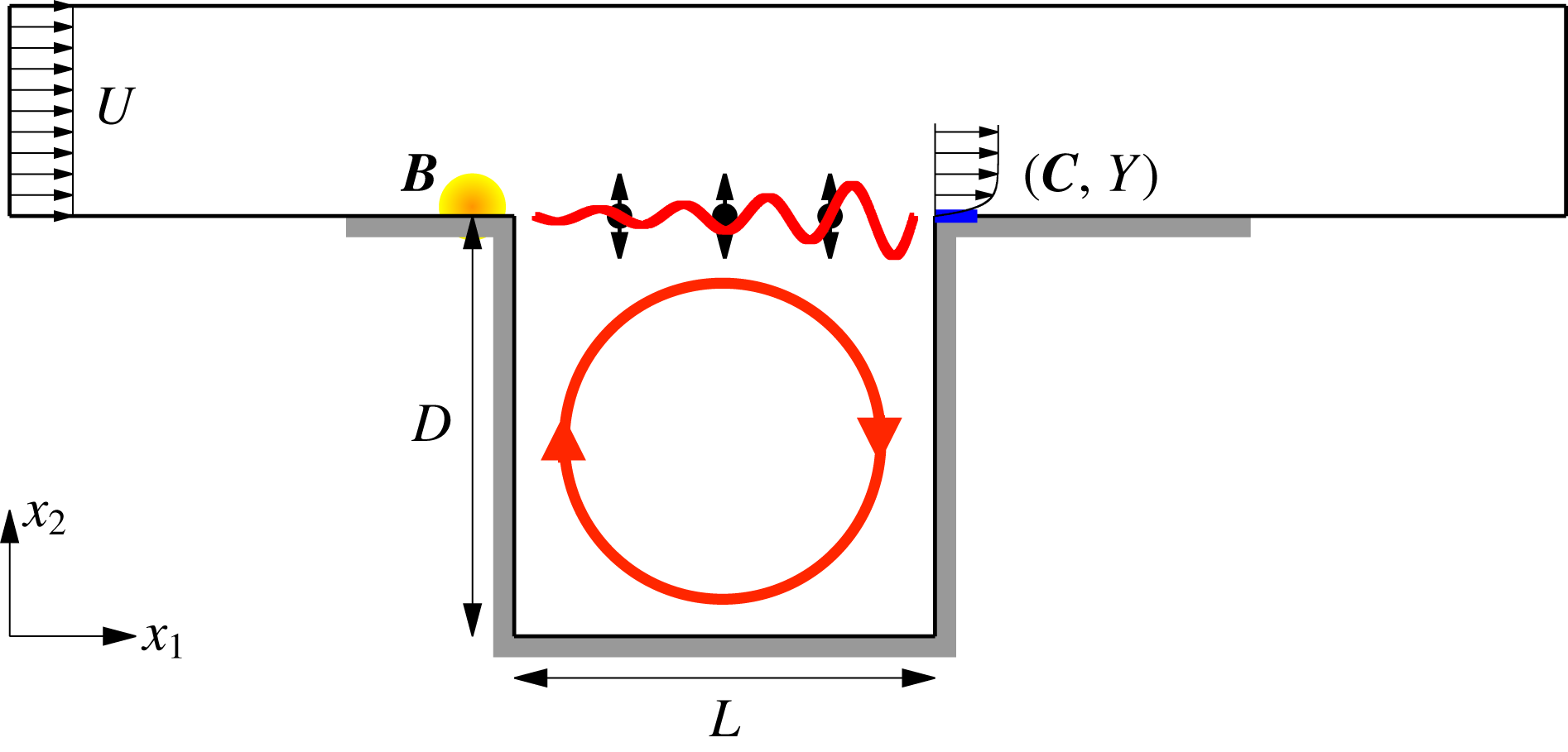
In the present paper, we propose to control the fully developed flow over a globally unstable open cavity, using the resolvent operator about the mean flow and a feedback-loop set-up (see figure 1 and §§3.1–3.2 for a comprehensive description of the model). The configuration under study has a unique fixed point, the base flow, which is unstable at the operating Reynolds number of
 $Re=7500$
. As we shall see in this paper, the system naturally evolves towards a quasiperiodic regime with two fundamental incommensurate frequencies (2-torus). Our aim is to bring the system back to the base flow, using sole knowledge of the mean flow, a single probe, a single actuator and linear methods only. The resolvent operator about the mean flow will be used to model the transfer function of the fully developed flow, while modal analysis will be used to interpret the results and guide the design of a robust linear controller, in the framework of structured
 ${\mathcal{H}}_{\infty }$
synthesis (Apkarian & Noll Reference Apkarian and Noll2006). As the controlled flow latches onto a new dynamical equilibrium, which is not the expected base flow, we will iterate the method on the new mean flow, and so on with subsequent mean states, until convergence. The choice of open-cavity flow is motivated by its frequent occurrence in the literature, as a convenient test-bed for validating new ideas; the cavity flow model used in this paper, in particular, has been used in many past studies (Rowley et al.
Reference Rowley, Williams, Colonius, Murray and Macmynowski2006; Sipp & Lebedev Reference Sipp and Lebedev2007; Barbagallo et al.
Reference Barbagallo, Sipp and Schmid2009; Barbagallo, Sipp & Schmid Reference Barbagallo, Sipp and Schmid2011; Dergham et al.
Reference Dergham, Sipp, Robinet and Barbagallo2011; Illingworth, Morgans & Rowley Reference Illingworth, Morgans and Rowley2012; Poussot-Vassal & Sipp Reference Poussot-Vassal and Sipp2015; Schmid & Sipp Reference Schmid and Sipp2016; Sipp & Schmid Reference Sipp and Schmid2016). Open-cavity flow also has many practical applications, in particular in the aerospace field: weapon bays, wheel wells and fuselage openings for telescopes and sensors, etc. (Rowley & Williams Reference Rowley and Williams2006; Cattafesta III et al.
Reference Cattafesta, Song, Williams, Rowley and Alvi2008).
Numerical model of open-cavity flow, with upstream (volume force) actuator
 $\boldsymbol{B}$
(in yellow) and downstream (shear-stress) sensor
 $(\boldsymbol{C},Y)$
(in blue). The shear-layer instability and cavity recirculation are symbolized with red lines. There are three
 $x_{2}$
-velocity probes in the shear layer at
 $x_{2}=0$
and respectively
 $x_{1}=1/4,1/2,3/4$
. Grey thick lines indicate no-slip boundary conditions.

The plan of the paper is as follows. In § 2, we introduce the theoretical framework for our iterative control strategy. In § 3, we present the cavity flow set-up and describe the uncontrolled dynamics. The design methodology for the first controller is then explained in § 4. The controlled flow is analysed in § 5 and a short discussion section follows in § 6. Finally, the main results are recalled in the conclusion § 7.
2 Theoretical framework
In this section, we cast the governing laws of motion in an input–output form convenient for feedback control. We then introduce a novel iterative method for stabilizing linearly unstable flows with a sequence of linear models and controllers. The methodology for designing robust controllers is explained later in § 4.
2.1 The Navier–Stokes equations as a Lur’e system
We start by considering the non-dimensional, incompressible, Navier–Stokes equations governing the velocity and pressure fields
 $\boldsymbol{u}$
and
 $p$
 $$\begin{eqnarray}\unicode[STIX]{x2202}_{t}\boldsymbol{u}+(\boldsymbol{u}\boldsymbol{\cdot }\unicode[STIX]{x1D735})\boldsymbol{u}=-\unicode[STIX]{x1D735}p+Re^{-1}\unicode[STIX]{x1D6FB}^{2}\boldsymbol{u},\quad \unicode[STIX]{x1D735}\boldsymbol{\cdot }\boldsymbol{u}=0,\end{eqnarray}$$
without external forcing. The Reynolds number
 $Re:=UL/\unicode[STIX]{x1D708}$
is based on characteristic velocity and length scales
 $U$
and
 $L$
of the problem, and on the kinematic viscosity
 $\unicode[STIX]{x1D708}$
of the fluid. Equations (2.1) are, of course, supplemented by appropriate boundary conditions and an initial condition. Next, we decompose the unknown field
 $\boldsymbol{q}:=(\boldsymbol{u},p)^{\text{T}}$
(
 $^{\text{T}}$
denoting the transpose) into an arbitrary steady incompressible reference field
 $\boldsymbol{Q}:=(\boldsymbol{U},P)^{\text{T}}$
satisfying the boundary conditions and a perturbation
 $\boldsymbol{q}^{\prime }:=(\boldsymbol{u}^{\prime },p^{\prime })^{\text{T}}$
with zero boundary conditions, such that
 $\boldsymbol{q}=\boldsymbol{Q}+\boldsymbol{q}^{\prime }$
. The unsteady perturbation
 $\boldsymbol{q}^{\prime }$
is governed by the following time-evolution equation
 $$\begin{eqnarray}{\mathcal{B}}\unicode[STIX]{x2202}_{t}\boldsymbol{q}^{\prime }=[{\mathcal{A}}_{\boldsymbol{ Q}}+\unicode[STIX]{x1D6F9}_{\boldsymbol{Q}}]\boldsymbol{q}^{\prime },\end{eqnarray}$$
where
 $$\begin{eqnarray}\displaystyle & \displaystyle {\mathcal{B}}\boldsymbol{q}^{\prime }:=\left(\begin{array}{@{}c@{}}\unicode[STIX]{x2202}_{t}\boldsymbol{u}^{\prime }\\ 0\end{array}\right), & \displaystyle\end{eqnarray}$$
 $$\begin{eqnarray}\displaystyle & \displaystyle {\mathcal{A}}_{\boldsymbol{Q}}\boldsymbol{q}^{\prime }:=\left(\begin{array}{@{}c@{}}-(\boldsymbol{U}\boldsymbol{\cdot }\unicode[STIX]{x1D735})\boldsymbol{u}^{\prime }-(\boldsymbol{u}^{\prime }\boldsymbol{\cdot }\unicode[STIX]{x1D735})\boldsymbol{U}+Re^{-1}\unicode[STIX]{x1D6FB}^{2}\boldsymbol{u}^{\prime }-\unicode[STIX]{x1D735}p^{\prime }\\ \unicode[STIX]{x1D735}\boldsymbol{\cdot }\boldsymbol{u}^{\prime }\end{array}\right), & \displaystyle\end{eqnarray}$$
 $$\begin{eqnarray}\displaystyle & \displaystyle \unicode[STIX]{x1D6F9}_{\boldsymbol{Q}}\boldsymbol{q}^{\prime }:=\left(\begin{array}{@{}c@{}}-(\boldsymbol{U}\boldsymbol{\cdot }\unicode[STIX]{x1D735})\boldsymbol{U}-\unicode[STIX]{x1D735}P+Re^{-1}\unicode[STIX]{x1D6FB}^{2}\boldsymbol{U}-(\boldsymbol{u}^{\prime }\boldsymbol{\cdot }\unicode[STIX]{x1D735})\boldsymbol{u}^{\prime }\\ 0\end{array}\right). & \displaystyle\end{eqnarray}$$
The Jacobian
 ${\mathcal{A}}_{\boldsymbol{Q}}$
and the operator
 $\unicode[STIX]{x1D6F9}_{\boldsymbol{Q}}$
respectively account for the linear and nonlinear parts of the evolution operator associated with the flow. Since
 $\boldsymbol{Q}$
is assumed to be time independent, the dynamical system is autonomous;
 ${\mathcal{A}}_{\boldsymbol{Q}}$
is a linear time-invariant (LTI) operator and
 $\unicode[STIX]{x1D6F9}_{\boldsymbol{Q}}$
is a static nonlinearity. Taking the Laplace transform of (2.2) leads to the relation
 $$\begin{eqnarray}\boldsymbol{q}^{\prime }(s)={\mathcal{R}}_{\boldsymbol{ Q}}(s)[\unicode[STIX]{x1D6F9}_{\boldsymbol{Q}}\boldsymbol{q}^{\prime }(s)+{\mathcal{B}}\boldsymbol{q}_{t=0}^{\prime }],\end{eqnarray}$$
where
 $s$
is the Laplace variable,
 $\boldsymbol{q}_{t=0}^{\prime }$
is the initial condition on the perturbation and
 $$\begin{eqnarray}{\mathcal{R}}_{\boldsymbol{Q}}(s):=(s{\mathcal{B}}-{\mathcal{A}}_{\boldsymbol{Q}})^{-1}\end{eqnarray}$$
is called the resolvent operator about the reference field
 $\boldsymbol{Q}$
. Such interconnection of an LTI operator
 ${\mathcal{R}}_{\boldsymbol{Q}}$
with a static nonlinearity
 $\unicode[STIX]{x1D6F9}_{\boldsymbol{Q}}$
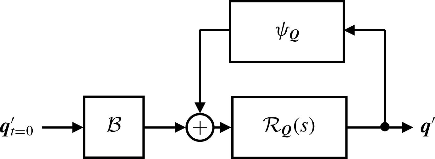
, illustrated in figure 2, is called a Lur’e system in nonlinear control theory (Khalil Reference Khalil2002; Sharma Reference Sharma2009; McKeon & Sharma Reference McKeon and Sharma2010).
The Navier–Stokes equations as a Lur’e system.

The resolvent operator is defined for any
 $s$
which is not an eigenvalue of the Jacobian operator, i.e. a solution of
 $$\begin{eqnarray}(s{\mathcal{B}}-{\mathcal{A}}_{\boldsymbol{Q}})\boldsymbol{q}^{\prime }=0,\end{eqnarray}$$
with non-zero
 $\boldsymbol{q}^{\prime }$
. Interestingly, the output
 $\boldsymbol{q}^{\prime }$
remains bounded even if
 ${\mathcal{A}}_{\boldsymbol{Q}}$
has unstable eigenvalues, thanks to the presence of the nonlinear feedback operator. Moreover, we stress that the resolvent operator itself is well defined along the imaginary axis as long as
 ${\mathcal{A}}_{\boldsymbol{Q}}$
has no marginally unstable eigenvalues. The choice of the arbitrary reference field
 $\boldsymbol{Q}$
is discussed in the next paragraph.
2.2 Open-loop and closed-loop transfer functions of fully developed flows
Block diagram of the forced Navier–Stokes equations in the (a) open-loop case and the (c) closed-loop case. Equivalent representation with an open-loop transfer function
 $G_{\boldsymbol{Q}}$
from
 $n$
to
 $y$
and an output disturbance
 $w$
in (b) the open loop and (d) the closed loop.

In figure 3(a,c), we now consider the effect of external forcing due to an actuator and modelled by a time-independent spatial field
 $\boldsymbol{B}$
multiplied by a time-varying scalar amplitude
 $n$
switched on at
 $t=0$
. We also introduce a sensor characterized by the time-independent pair
 $(\boldsymbol{C},Y)$
providing the local measurement
 $$\begin{eqnarray}y(t):=\langle \boldsymbol{C},\boldsymbol{q}^{\prime }(t)\rangle +Y,\end{eqnarray}$$
where
 $$\begin{eqnarray}\langle \boldsymbol{q}_{1},\boldsymbol{q}_{2}\rangle :=\int _{{\mathcal{D}}}\boldsymbol{q}_{1}^{\ast }\boldsymbol{\cdot }\boldsymbol{q}_{2}\,\text{d}{\mathcal{D}}\end{eqnarray}$$
defines an inner product over the domain
 ${\mathcal{D}}$
and
 $^{\ast }$
denotes complex conjugation. The output
 $y$
is linear with respect to the fluctuation
 $\boldsymbol{q}^{\prime }$
and the constant
 $Y$
represents an arbitrary offset. Panel (a) represents the case of open-loop forcing, while panel (c) represents a feedback-loop configuration with a total actuation amplitude
 $u+n$
, where
 $$\begin{eqnarray}u:=Ky\end{eqnarray}$$
is due to an LTI controller of transfer function
 $K(s)$
. With external forcing, the output
 $\boldsymbol{q}^{\prime }$
is respectively given by
 $$\begin{eqnarray}\boldsymbol{q}^{\prime }={\mathcal{R}}_{\boldsymbol{ Q}}[\unicode[STIX]{x1D6F9}_{\boldsymbol{Q}}\boldsymbol{q}^{\prime }+{\mathcal{B}}\boldsymbol{q}_{t=0}^{\prime }+\boldsymbol{B}n]\end{eqnarray}$$
in the open-loop case, and
 $$\begin{eqnarray}\boldsymbol{q}^{\prime }=({\mathcal{I}}-{\mathcal{R}}_{\boldsymbol{ Q}}\boldsymbol{B}K\langle \boldsymbol{C},\boldsymbol{\cdot }\rangle )^{-1}{\mathcal{R}}_{\boldsymbol{Q}}\left[\unicode[STIX]{x1D6F9}_{\boldsymbol{Q}}\boldsymbol{q}^{\prime }+{\mathcal{B}}\boldsymbol{q}_{t=0}^{\prime }+\boldsymbol{B}n+\boldsymbol{B}K{\displaystyle \frac{Y}{s}}\right]\end{eqnarray}$$
in the closed-loop case. The latter expression can be rewritten as
 $$\begin{eqnarray}\boldsymbol{q}^{\prime }={\mathcal{R}}_{\boldsymbol{ Q}}^{K}\left[\unicode[STIX]{x1D6F9}_{\boldsymbol{Q}}\boldsymbol{q}^{\prime }+{\mathcal{B}}\boldsymbol{q}_{t=0}^{\prime }+\boldsymbol{B}n+\boldsymbol{B}K{\displaystyle \frac{Y}{s}}\right],\end{eqnarray}$$
where
 $$\begin{eqnarray}{\mathcal{R}}_{\boldsymbol{Q}}^{K}(s):=(s{\mathcal{B}}-{\mathcal{A}}_{\boldsymbol{ Q}}^{K}(s))^{-1}\end{eqnarray}$$
is the resolvent operator associated with the Jacobian operator
 $$\begin{eqnarray}{\mathcal{A}}_{\boldsymbol{Q}}^{K}(s):={\mathcal{A}}_{\boldsymbol{ Q}}+K(s)\boldsymbol{B}\langle \boldsymbol{C},.\rangle\end{eqnarray}$$
of the coupled system fluid/controller. Because of the nonlinear feedback term, the concept of a transfer function from
 $n$
to
 $\boldsymbol{q}^{\prime }$
is ill defined. However, using the resolvent operators introduced above and lumping all the terms independent of
 $n$
in an output disturbance term
 $\boldsymbol{w}$
, we can recast the governing equations (2.12) and (2.14) in a form that resembles input–output relations:
 $$\begin{eqnarray}\boldsymbol{q}^{\prime }={\mathcal{R}}_{\boldsymbol{ Q}}\boldsymbol{B}n+\boldsymbol{w}\quad \text{and}\quad \boldsymbol{q}^{\prime }={\mathcal{R}}_{\boldsymbol{ Q}}^{K}\boldsymbol{B}n+\boldsymbol{w}\end{eqnarray}$$
in the open-loop and closed-loop cases respectively. Similar to the unforced case, the output
 $\boldsymbol{q}^{\prime }$
is bounded despite the potential presence of unstable eigenvalues in
 ${\mathcal{A}}_{\boldsymbol{Q}}$
or
 ${\mathcal{A}}_{\boldsymbol{Q}}^{K}$
, thanks to the nonlinear feedback term (included in
 $\boldsymbol{w}$
) ensuring saturation.
An important point to note at this point is that the definition of the Lur’e system associated with the flow depends on the arbitrary choice of a steady reference field
 $\boldsymbol{Q}$
. The passivity theorem states that if the two interconnected blocks
 ${\mathcal{R}}_{\boldsymbol{Q}}^{K}$
and
 $\unicode[STIX]{x1D6F9}_{\boldsymbol{Q}}$
are passive, i.e. can only store or dissipate energy, then the fixed point of the closed loop is stable with respect to perturbations of any amplitude. For
 $\boldsymbol{Q}=\boldsymbol{q}_{b}$
, the static nonlinearity
 $$\begin{eqnarray}\unicode[STIX]{x1D6F9}_{\boldsymbol{q}_{b}}\boldsymbol{q}^{\prime }=\left(\begin{array}{@{}c@{}}-(\boldsymbol{u}^{\prime }\boldsymbol{\cdot }\unicode[STIX]{x1D735})\boldsymbol{u}^{\prime }\\ 0\end{array}\right)\end{eqnarray}$$
happens to be conservative, hence passive. Therefore, a possible strategy to reach the base flow from the regime of fully developed oscillations consists in designing an LTI feedback controller making the closed-loop linear dynamics about the base flow passive. That means designing a controller
 $K$
suppressing both modal growth and transient growth arising from the non-normality of the Jacobian operator
 ${\mathcal{A}}_{\boldsymbol{q}_{b}}$
. This strategy has been pursued in recent works by Sharma et al. (Reference Sharma, Morrison, McKeon, Limebeer, Koberg and Sherwin2011) and Heins et al. (Reference Heins, Jones and Sharma2016), for globally stable flows (i.e. no modal growth). However, as discussed in the introduction, the resolvent operator about the mean flow appears to be a better choice for describing the behaviour of unforced flows in the fully developed regime. McKeon & Sharma (Reference McKeon and Sharma2010) therefore proposed to consider the mean flow
 $\overline{\boldsymbol{q}}$
as an appropriate alternative choice of reference field
 $\boldsymbol{Q}$
in (2.6), in order to define the unforced Navier–Stokes as a Lur’e system. In that case, the nonlinear output
 $$\begin{eqnarray}\unicode[STIX]{x1D6F9}_{\overline{\boldsymbol{q}}}\boldsymbol{q}^{\prime }=\left(\begin{array}{@{}c@{}}\overline{(\boldsymbol{u}^{\prime }\boldsymbol{\cdot }\unicode[STIX]{x1D735})\boldsymbol{u}^{\prime }}-(\boldsymbol{u}^{\prime }\boldsymbol{\cdot }\unicode[STIX]{x1D735})\boldsymbol{u}^{\prime }\\ 0\end{array}\right)\end{eqnarray}$$
was interpreted as an endogenous forcing term. We decide to follow the same approach here and also choose
 $$\begin{eqnarray}\boldsymbol{Q}:=\overline{\boldsymbol{q}}\end{eqnarray}$$
to model the flow receptivity to the exogenous forcing field
 $\boldsymbol{B}$
.
In the case of unforced flows, the mean flow is unambiguously defined as the temporal average of
 $\boldsymbol{q}$
in the fully developed regime. The case of externally forced flow is not as straightforward, as starting the forcing at
 $t=0$
(either
 $u$
or
 $n$
) triggers nonlinear effects which lead to a change in the flow dynamics. Instead of one, we have two relevant mean flows: (i) that associated with the initial attractor characterizing the unforced system at
 $t=0$
, and (ii) that characterizing the final attractor of the forced system as
 $t\rightarrow \infty$
. During the transient, the mean flow is not defined. If we want to extend the framework of McKeon & Sharma (Reference McKeon and Sharma2010) to externally forced flows, we therefore need to be very careful about choosing the appropriate reference mean flow. Using the resolvent operator about the mean flow, we can only derive input–output models relevant at the initial and final times. In the open-loop case, we simply have
 $$\begin{eqnarray}y=G_{\overline{\boldsymbol{q}}}n+w,\end{eqnarray}$$
where
 $$\begin{eqnarray}G_{\overline{\boldsymbol{q}}}(s):=\langle \boldsymbol{C},{\mathcal{R}}_{\overline{\boldsymbol{q}}}(s)\boldsymbol{B}\rangle\end{eqnarray}$$
models the transfer function from
 $n$
to
 $y$
and
 $w$
collects the various remaining terms in the form of an ‘output disturbance’. This simple relation is represented by the block diagram in figure 3(b). In the closed-loop case, the transfer function model becomes
 $$\begin{eqnarray}G_{\overline{\boldsymbol{q}}}^{K}(s):=\langle \boldsymbol{C},{\mathcal{R}}_{\overline{\boldsymbol{q}}}^{K}(s)\boldsymbol{B}\rangle\end{eqnarray}$$
and depends on both
 $\overline{\boldsymbol{q}}$
and the controller
 $K$
. This pseudo-transfer function can also be computed from the expression
 $$\begin{eqnarray}G_{\overline{\boldsymbol{q}}}^{K}={\displaystyle \frac{G_{\overline{\boldsymbol{q}}}}{1-G_{\overline{\boldsymbol{q}}}K}},\end{eqnarray}$$
which corresponds to the linear plant
 $G_{\overline{\boldsymbol{q}}}$
in the feedback loop with the controller
 $K$
, as can be seen in figure 3(d). The reference field
 $\overline{\boldsymbol{q}}$
either characterizes the mean flow of the initial attractor or the final attractor. The discrete evolution of the reference mean flow, and therefore of the input–output model of the system as we add control action, may be used to design an iterative control strategy as explained below.
2.3 Iterative control strategy
In this section, we introduce an iterative control strategy to reach the base flow from the permanent regime of oscillation of an uncontrolled resonating flow. Assume we know how to design a first controller
 $K_{1}$
able to decrease the amplitude of oscillation of the unforced flow, but unable to completely stabilize it, can we design a controller correction
 $K_{2}^{\prime }$
such that the total controller
 $K_{2}:=K_{1}+K_{2}^{\prime }$
is able to damp the oscillations further? In general, from a sequence of
 $m$
successive controller corrections
 $$\begin{eqnarray}K_{m}:=\left\{\begin{array}{@{}ll@{}}0,\quad & \text{if }m=0,\\ K_{1}^{\prime }+K_{2}^{\prime }+\cdots +K_{m}^{\prime },\quad & \text{if }m>0,\end{array}\right.\end{eqnarray}$$
leading to a permanent oscillatory regime, how can we design the next controller correction
 $K_{m+1}^{\prime }$
such that
 $K_{m+1}=K_{m}+K_{m+1}^{\prime }$
leads to even smaller oscillation amplitude?
The key idea is to consider an input–output model based on the mean flow
 $\overline{\boldsymbol{q}}_{m}$
obtained in the presence of the controller
 $K_{m}$
. Indeed, as shown in the previous section, the response of the coupled system to a perturbation
 $n$
of the forcing signal is given by the resolvent operator
 ${\mathcal{R}}_{\overline{\boldsymbol{q}}_{m}}^{K_{m}}$
, involving both
 $\overline{\boldsymbol{q}}_{m}$
and
 $K_{m}$
. The corresponding transfer function from
 $n$
to
 $y$
is then given by
 $G_{\overline{\boldsymbol{q}}_{m}}^{K_{m}}$
. To simplify notations, we denote from now on
 $$\begin{eqnarray}G_{i}^{j}:=G_{\overline{\boldsymbol{q}}_{i}}^{K_{j}}.\end{eqnarray}$$
At each step
 $m+1$
, the plant to control is therefore denoted
 $G_{m}^{m}$
. The goal is to design a controller correction
 $K_{m+1}^{\prime }$
such that the target plant
 $$\begin{eqnarray}G_{m}^{m+1}={\displaystyle \frac{G_{m}^{m}}{1-G_{m}^{m}K_{m+1}^{\prime }}}\end{eqnarray}$$
has some desired properties, leading to smaller oscillations of the output
 $y$
. When the additional controller
 $K_{m+1}^{\prime }$
is added in the feedback loop, the flow transiently evolves until a new dynamical equilibrium is reached, characterized by a new mean state
 $\overline{\boldsymbol{q}}_{m+1}$
. Since the effective controller is now
 $K_{m+1}=K_{m}+K_{m+1}^{\prime }$
, the transfer function of the new plant is
 $G_{m+1}^{m+1}$
. The iteration then proceeds until convergence, i.e. until some fixed point is hopefully reached.
Evolution of the block diagram representation of the system during the iterative procedure: (a)
 $t=t_{1}^{+}$
,
 $K_{1}^{\prime }$
has just been added so the flow alone is still characterized by the plant
 $G_{0}^{0}$
; (b)
 $t=t_{2}^{-}$
the feedback loop between the fluid and the controller
 $K_{1}:=K_{1}^{\prime }$
has converged to a new mean state; (c)
 $t=t_{2}^{+}$
,
 $K_{2}^{\prime }$
has just been added so the flow alone is still characterized by the plant
 $G_{1}^{0}$
; (d)
 $t=t_{2}^{-}$
the feedback loop between the fluid and the controller
 $K_{2}:=K_{1}^{\prime }+K_{2}^{\prime }$
has converged to a new mean state.

The momentum equation with feedback reads
 $$\begin{eqnarray}\unicode[STIX]{x2202}_{t}\boldsymbol{u}+(\boldsymbol{u}\boldsymbol{\cdot }\unicode[STIX]{x1D735})\boldsymbol{u}=-\unicode[STIX]{x1D735}p+Re^{-1}\unicode[STIX]{x1D6FB}^{2}\boldsymbol{u}+\boldsymbol{B}_{\boldsymbol{ u}}\int _{0}^{t}\unicode[STIX]{x1D705}_{m}(\unicode[STIX]{x1D70F})y(t-\unicode[STIX]{x1D70F})\,\text{d}\unicode[STIX]{x1D70F},\end{eqnarray}$$
where
 $\boldsymbol{B}_{\boldsymbol{u}}$
is the component of
 $\boldsymbol{B}$
forcing the momentum equation and
 $\unicode[STIX]{x1D705}_{m}$
is the impulse response of the controller
 $K_{m}$
. If a fixed point
 $\boldsymbol{q}_{\infty }:=(\boldsymbol{u}_{\infty },p_{\infty })$
is reached in the limit
 $t\rightarrow \infty$
, then it must satisfy
 $$\begin{eqnarray}(\boldsymbol{u}_{\infty }\boldsymbol{\cdot }\unicode[STIX]{x1D735})\boldsymbol{u}_{\infty }=-\unicode[STIX]{x1D735}p_{\infty }+Re^{-1}\unicode[STIX]{x1D6FB}^{2}\boldsymbol{u}_{\infty }+\boldsymbol{B}_{\boldsymbol{u}}K_{m}(0)(\langle \boldsymbol{C},\boldsymbol{q}_{\infty }-\boldsymbol{Q}\rangle +Y).\end{eqnarray}$$
In order to reach the base flow, i.e.
 $\boldsymbol{q}_{\infty }=\boldsymbol{q}_{b}$
, we must ensure that
 $\boldsymbol{q}_{b}$
is a solution of (2.29), and that it is the only one. This is the case if the controller has zero static gain
 $K_{m}(0)=0$
, and we therefore choose to impose
 $$\begin{eqnarray}K_{j}^{\prime }(0)=0\end{eqnarray}$$
at every step
 $j$
. In the special case where the sensor measures a deviation with respect to the base flow by satisfying
 $$\begin{eqnarray}Y=\langle \boldsymbol{C},\boldsymbol{Q}-\boldsymbol{q}_{b}\rangle ,\end{eqnarray}$$
then
 $\boldsymbol{q}_{b}$
remains a fixed point of (2.29) even if
 $K_{m}(0)\neq 0$
, but there may be alternative fixed points
 $\boldsymbol{q}_{\infty }$
as well. It is therefore crucial to ‘disconnect’ the controller in the steady regime by imposing (2.30); then
 $\boldsymbol{q}_{b}$
is for sure the only fixed point for any choice of sensor
 $(\boldsymbol{C},Y)$
.
Although the iterative method bears resemblance to the gain scheduling approach of Khalil (Reference Khalil2002) and Högberg, Bewley & Henningson (Reference Högberg, Bewley and Henningson2003), there are fundamental differences which are emphasized later in the discussion, see § 6.2. We stress again that the concept of a transfer function from
 $n$
to
 $y$
is ill defined in the context of nonlinear flows. Our method relies on the assumption that the system responds to external forcing in a LTI fashion when it is close to a state of dynamical equilibrium. The quantity that we will call ‘transfer function’, and that we will denote
 $G$
in general, is therefore only defined in two limit cases: either (i) the system is in a dynamical equilibrium characterized by
 $\overline{\boldsymbol{q}}_{m}$
and
 $K_{m}$
, or (ii) the system is out of equilibrium because a controller correction
 $K_{m+1}^{\prime }$
has just been added, but the flow has not yet evolved so the mean flow
 $\overline{\boldsymbol{q}}_{m}$
remains relevant over some period of time. Denoting
 $t_{m+1}$
the instant when the controller correction
 $K_{m+1}^{\prime }$
is added, we have
 $G=G_{m}^{m}$
at
 $t=t_{m+1}^{-}$
and
 $G=G_{m}^{m+1}$
at
 $t=t_{m+1}^{+}$
. And then we reach
 $G=G_{m+1}^{m+1}$
at
 $t=t_{m+2}^{-}$
. But between the two instants
 $t_{m+1}$
and
 $t_{m+2}$
, the transfer function model
 $G$
cannot be defined as there is no mean state relevant to the transiently evolving flow.
Finally, according to (2.24) and (2.25), each transfer function
 $G_{i}^{j}$
can be seen as the interconnection
 $$\begin{eqnarray}G_{i}^{j}={\displaystyle \frac{G_{i}^{0}}{1-G_{i}^{0}(K_{1}^{\prime }+\cdots +K_{j}^{\prime })}}\end{eqnarray}$$
between the plant
 $G_{i}^{0}$
characterizing the mean flow alone (even though it cannot be sustained without controllers for
 $i\neq 0$
), and the controller corrections
 $K_{1}^{\prime }$
to
 $K_{j}^{\prime }$
plugged in parallel. The block diagrams at times
 $t=t_{1}^{+}$
,
 $t_{2}^{\pm }$
and
 $t_{3}^{-}$
are shown in figure 4.
2.4 Relation between poles of the transfer operators
 $G_{i}^{j}$
and instability modes

In the present context, modal analysis of the Jacobian operator
 ${\mathcal{A}}_{i}^{j}$
is used to find the pole singularities of the resolvent operator
 ${\mathcal{R}}_{i}^{j}$
(with obvious notations), and therefore of the transfer function
 $G_{i}^{j}$
. We are concerned with the solutions of the generalized eigenvalue problem
 $$\begin{eqnarray}(s_{l}{\mathcal{B}}-{\mathcal{A}}_{i}^{j}(s_{l}))\boldsymbol{q}_{l}^{\prime }=0,\end{eqnarray}$$
with complex eigenvalues
 $s_{l}=\text{i}\unicode[STIX]{x1D714}_{l}+\unicode[STIX]{x1D70E}_{l}$
of growth rate
 $\unicode[STIX]{x1D70E}_{l}$
, frequency
 $\unicode[STIX]{x1D714}_{l}$
and eigenmodes
 $\boldsymbol{q}_{l}^{\prime }$
(the method used to obtain approximate solutions of (2.33) will be explained in § 4.1). In our case, resonant frequencies will be associated with specific eigenmodes of the mean flow
 $\overline{\boldsymbol{q}}_{i}$
, coupled with controller
 $K_{j}$
. These modes cannot be directly interpreted as instability modes if the mean flow is different from the base flow. However, the Jacobian operator
 ${\mathcal{A}}_{i}^{j}$
may be seen as a perturbation of operator
 ${\mathcal{A}}_{i}^{0}$
with a correction term proportional to
 $K_{j}$
according to (2.16), i.e.
 $$\begin{eqnarray}{\mathcal{A}}_{i}^{j}={\mathcal{A}}_{i}^{0}+K_{j}\boldsymbol{B}\langle \boldsymbol{C},\boldsymbol{\cdot }\rangle .\end{eqnarray}$$
A continuous connection can therefore be established between the eigenvalues of the two operators. The Jacobian operator
 ${\mathcal{A}}_{i}^{0}$
may in turn be seen as a perturbation of the Jacobian operator about the base flow
 ${\mathcal{A}}_{\boldsymbol{q}_{b}}^{0}$
, with a correction term due to mean-flow distortion
 $\unicode[STIX]{x0394}\overline{\boldsymbol{q}}_{i}$
, where
 $$\begin{eqnarray}\unicode[STIX]{x0394}\boldsymbol{q}:=\boldsymbol{q}-\boldsymbol{q}_{b}.\end{eqnarray}$$
Therefore, all instability modes of the base flow may be unambiguously identified with some poles of
 $G_{i}^{j}$
, thereby providing the latter with a physical meaning. This key advantage of our resolvent-based model will be illustrated in § 3.5.
3 Unforced flow
3.1 Numerical model and methods
The control strategy is implemented on a well-known open-cavity flow configuration, which was considered in a series of past papers (Barbagallo et al.
Reference Barbagallo, Sipp and Schmid2009, Reference Barbagallo, Sipp and Schmid2011; Dergham et al.
Reference Dergham, Sipp, Robinet and Barbagallo2011; Poussot-Vassal & Sipp Reference Poussot-Vassal and Sipp2015; Schmid & Sipp Reference Schmid and Sipp2016; Sipp & Schmid Reference Sipp and Schmid2016) following Sipp & Lebedev (Reference Sipp and Lebedev2007). The reader is referred to this initial paper for a comprehensive description of the numerical set-up. The cavity of length
 $L=1$
and depth
 $D$
has an aspect ratio
 $L/D=1$
, as shown in figure 1. In the Cartesian coordinate system
 $(x_{1},x_{2})$
, the velocity components are denoted
 $\boldsymbol{u}=(u_{1},u_{2})$
. With the upstream edge of the cavity defining the origin
 $(0,0)$
and the incoming flow aligned with the
 $x_{1}$
-direction, the upstream boundary layer starts forming at
 $x_{1}=-0.4$
by switching the lower-wall boundary condition from stress free
 $\unicode[STIX]{x2202}_{2}u_{1}=0$
to no slip
 $u_{1}=0$
(in both cases, the walls are impermeable, i.e.
 $u_{2}=0$
). The inlet velocity
 $(U=1,0)$
at
 $x_{1}=-1.2$
is uniform and a standard outflow condition is prescribed at the outlet, which is located at
 $x_{1}=2.5$
. A stress-free boundary condition is implemented on the upper wall at
 $x_{2}=0.5$
and at the downstream end of the lower wall, from
 $x_{1}=1.75$
to
 $x_{1}=2.5$
. The two-dimensional incompressible Navier–Stokes equations are solved using the freely available finite-element software FreeFem++ (www.freefem.org). The primitive variables
 $(u_{1},u_{2},p)$
are discretized on a mesh of
 ${\sim}200\,000$
 $(P1b,P1b,P1)$
Taylor–Hood elements, yielding a total of
 ${\sim}700\,000$
degrees of freedom. The time-stepping code, which was made available online (https://github.com/denissipp/AMR_Sipp_Schmid_2016) as complementary material to the review article by Sipp & Schmid (Reference Sipp and Schmid2016), is semi-implicit, with the nonlinear terms extrapolated with a second-order Adams–Bashforth scheme.
We consider the nonlinear dynamics of the linearly unstable flow at a Reynolds number of
 $Re=7500$
. The dynamical equilibrium that we consider for our control problem is obtained by initializing the simulation with the base flow
 $\boldsymbol{q}_{b}$
– which was computed using Newton’s iteration (Sipp & Schmid Reference Sipp and Schmid2016) – plus a small contribution from the most unstable linear mode. After a long transient, characterized in § 3.3, the flow reaches a quasiperiodic attractor, characterized in § 3.4.
Modal analyses were carried out using the ARPACK implementation of Arnoldi’s method (Lehoucq, Sorensen & Yang Reference Lehoucq, Sorensen and Yang1997), coupled with the multifrontal sparse LU solver MUMPS (Amestoy et al. Reference Amestoy, Duff, Koster and L’Excellent2001, Reference Amestoy, Guermouche, L’Excellent and Pralet2006). The shift-invert mode was used to find eigenvalues of the Jacobian operator in the vicinity of a given shift.
3.2 Actuator and flow measurements
The upstream-edge actuator is modelled by a Gaussian-shaped volume force term
 $$\begin{eqnarray}\boldsymbol{B}=\left[0,\unicode[STIX]{x1D702}\exp \left(-{\displaystyle \frac{(x_{1}-x_{1}^{0})^{2}+(x_{2}-x_{2}^{0})^{2}}{2\unicode[STIX]{x1D70E}^{2}}}\right),0\right]^{\text{T}},\end{eqnarray}$$
centred around
 $(x_{1}^{0},x_{2}^{0})=(-0.1,0.02)$
, with a scalar
 $\unicode[STIX]{x1D702}$
such that
 $\langle \boldsymbol{B},\boldsymbol{B}\rangle =1$
. With the choice of spatial variance
 $\unicode[STIX]{x1D70E}=0.0849$
, the volume force reaches
 $50\,\%$
of its maximum value at a radial distance of
 ${\approx}0.1$
from
 $(x_{1}^{0},x_{2}^{0})$
, and
 $1\,\%$
at
 ${\approx}0.26$
.
In order to characterize the strength of the nonlinearity, we define different measures of the distance between the instantaneous field
 $\boldsymbol{q}$
and the base flow
 $\boldsymbol{q}_{b}$
, based on the perturbation field
 $\unicode[STIX]{x0394}\boldsymbol{q}$
. The downstream-edge sensor is modelled by a pair
 $(\boldsymbol{C},Y)$
such that
 $$\begin{eqnarray}y=\left.\int _{x_{1}=1}^{1.1}\unicode[STIX]{x2202}_{2}\unicode[STIX]{x0394}u_{1}\right|_{x_{2}=0}\,\text{d}x_{1}\end{eqnarray}$$
measures the perturbation wall friction at the downstream edge of the cavity. Note that this sensor satisfies (2.31), hence the base flow is a fixed point of the closed-loop system, even if the controller has non-zero static gain. However, as discussed in § 2.3, we will still need to impose
 $K_{j}^{\prime }(0)=0$
at every iteration, in order to guarantee that there are no alternative fixed points.
In order to build phase portraits, we also consider three
 $x_{2}$
-perturbation velocity probes located within the shear layer at
 $x_{2}=0$
and
 $x_{1}=1/4,1/2,3/4$
. Finally, to characterize the system globally, we consider the perturbation kinetic energy
 $$\begin{eqnarray}E:={\displaystyle \frac{\langle \unicode[STIX]{x0394}\boldsymbol{q},{\mathcal{B}}\unicode[STIX]{x0394}\boldsymbol{q}\rangle }{\langle \boldsymbol{q}_{b},{\mathcal{B}}\boldsymbol{q}_{b}\rangle }}.\end{eqnarray}$$
3.3 Transient dynamics
Time series of (a–c) perturbation kinetic energy
 $E$
and (d–f) shear-stress measurement
 $y$
of the unforced flow, with sliding mean shown as a black dotted line. Zooms on the initial and final stages are shown in insets.

Figure 5 shows time series of the global and local measures
 $E$
and
 $y$
of the uncontrolled flow. We recall that the simulation is initialized with the base flow plus a small perturbation parallel to the most unstable base-flow eigenmode. There is a short initial phase of linear growth associated with that mode (see inset (a)), before saturating effects of nonlinearity become active. This phase lasts a few convective time units, after which the flow undergoes a long transient evolution of a few hundred time units before a dynamical equilibrium is eventually reached, that we call state 0. This state appears to contain multiple frequencies, as can be seen in insets (b) and (e). Mean-flow distortion is caused by nonlinear interactions between these finite-amplitude oscillatory modes. The deviation is significant since the mean value of
 $y$
is comparable with its oscillation amplitude, confirming strong nonlinearity. The mean perturbation energy
 $\overline{E}$
is of the order of
 $2\,\%$
(see figure 5
c), which corresponds to perturbation velocities of the order of
 $0.1$
.
3.4 Attractor
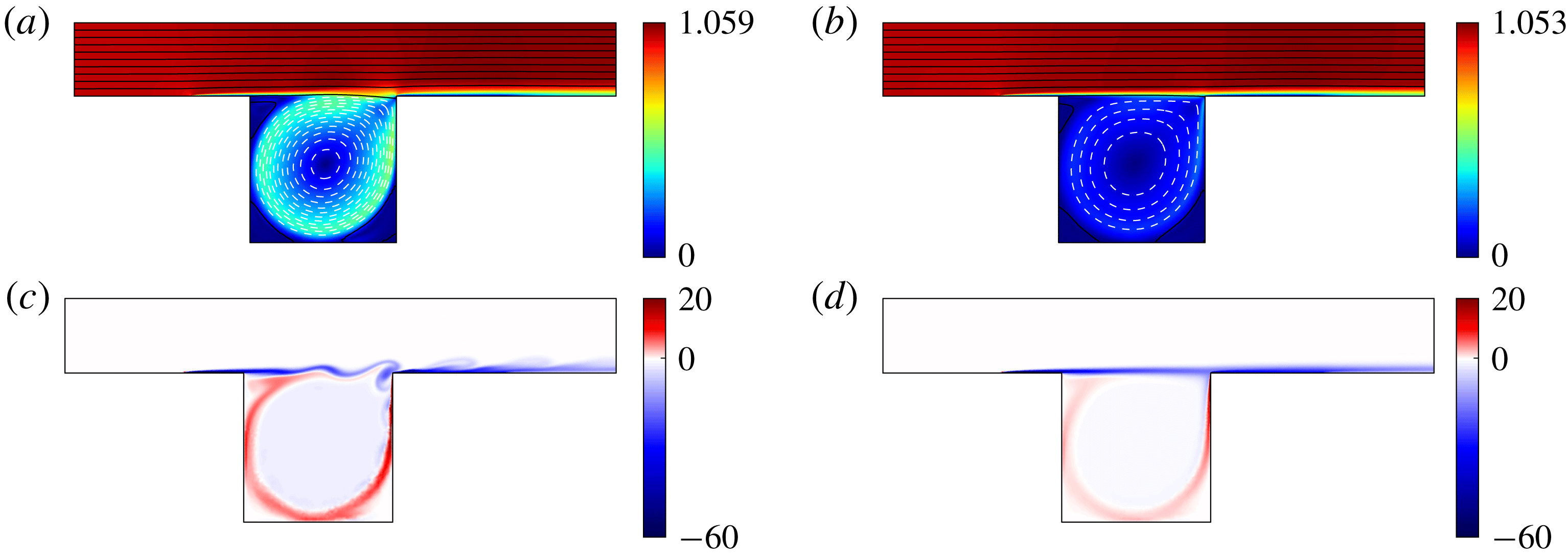
The resulting mean flow is shown in figure 6(a), together with the base flow in (b), for comparison. We display streamfunction contours on top of filled contours of the total velocity norm. The growth of a boundary layer at the lower wall is apparent from
 $x_{1}=-0.4$
. This boundary layer becomes a shear layer on top of the cavity, which thickens as it is convected towards the downstream edge. The flow recirculates at low speeds within the cavity, as the incoming flow impacts the downstream wall of the cavity. We note two main differences between mean and base flows: (a) the spreading of the shear layer is more pronounced for the mean flow, (b) from inspection of the streamlines, the recirculating flow rate is also stronger in that case. The enhanced flow rate is caused by stronger entrainment due to the unsteady shear layer.
Comparison between (a,c) state 0 and (b,d) the base flow. (a,b) Velocity 2-norm of (a) uncontrolled mean flow
 $\overline{\boldsymbol{u}}_{0}$
(computed by averaging over 200 time units, after the transient) and (b) base flow
 $\boldsymbol{u}_{b}$
, with associated contours of the streamfunction
 $\unicode[STIX]{x1D713}$
. The streamfunction is defined by the relations
 $\unicode[STIX]{x2202}_{2}\unicode[STIX]{x1D713}=v_{1}$
,
 $\unicode[STIX]{x2202}_{1}\unicode[STIX]{x1D713}=-v_{2}$
and
 $\unicode[STIX]{x1D713}=0$
on the lower wall (solid contours for positive increments
 $\unicode[STIX]{x1D6FF}\unicode[STIX]{x1D713}=0.05$
from
 $\unicode[STIX]{x1D713}=0$
; dashed contours for negative increments
 $\unicode[STIX]{x1D6FF}\unicode[STIX]{x1D713}=-0.01$
from
 $\unicode[STIX]{x1D713}=0$
). (c,d) Vorticity fields: (c) snapshot at a time of maximum shear stress
 $y$
at the downstream sensor and (d) base flow.

Figure 6(c) shows a vorticity snapshot of state 0 yielding maximal instantaneous shear stress
 $y$
, compared to the steady vorticity field of the base flow in (d). We notice the spatial development of the Kelvin–Helmholtz instability on top of the shear layer, which is responsible for its enhanced spreading in figure 6(a). The maximum shear stress is caused by the impact of a vortical structure at the downstream corner of the cavity. Another vorticity sheet of opposite sign is visible within the cavity, and marks the border of the recirculating zone. The vorticity levels within that sheet are higher in state 0 than in the base flow, which is consistent with the stronger recirculation in the former case. Finally, the average distance between the mean flow and any instantaneous snapshot measured as
 $\overline{\langle \boldsymbol{q}^{\prime },\boldsymbol{q}^{\prime }\rangle }/\langle \overline{\boldsymbol{q}}_{0},\overline{\boldsymbol{q}}_{0}\rangle \approx 1.1\times 10^{-3}$
is very low, so the mean flow can be considered as a good approximation of the full flow at any instant.
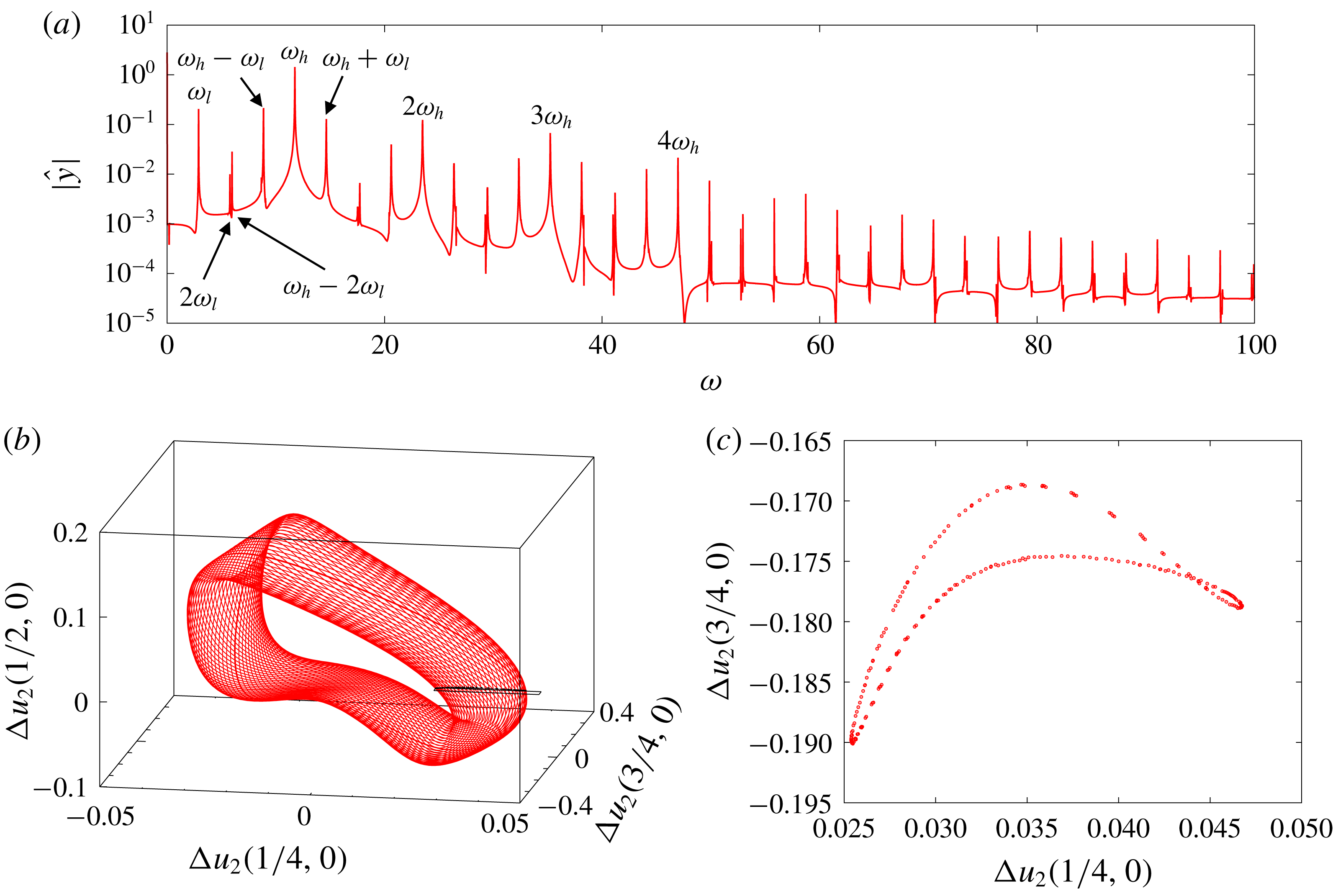
Characterization of the attractor without actuation: (a) spectrum of amplitude of the Koopman modes of
 $y$
, estimated using DFT over a finite time series of
 $300$
time units (no windowing), with frequency resolution
 $\unicode[STIX]{x0394}\unicode[STIX]{x1D714}\approx 2\times 10^{-2}$
; (b) phase portrait using three
 $x_{2}$
-velocity probes in the shear layer at
 $x_{2}=0$
and
 $x_{1}=1/4,1/2,3/4$
(see figure 1); (c) Poincaré section of (b) for
 $u_{2}(1/2,0)=0$
(crossing from below); the section plane is also indicated in (b). The three plots indicate quasiperiodic behaviour with two incommensurate frequencies (2-torus)
 $\unicode[STIX]{x1D714}_{l}\approx 2.89$
and
 $\unicode[STIX]{x1D714}_{h}\approx 11.74$
.

The dynamical state may be further characterized in the frequency domain by considering the spectrum of Koopman modes. For fully developed flows, these can be computed using harmonic averages
 $$\begin{eqnarray}\hat{\boldsymbol{q}}^{\prime }(\unicode[STIX]{x1D714}):=\lim _{T\rightarrow \infty }{\displaystyle \frac{1}{T}}\int _{0}^{T}\boldsymbol{q}^{\prime }(t)\text{e}^{-\text{i}\unicode[STIX]{x1D714}t}\,\text{d}t\end{eqnarray}$$
(Arbabi & Mezić Reference Arbabi and Mezić2017). The limit is non-zero for Koopman eigenfrequencies only, and yields the associated Koopman modes of the observable
 $\boldsymbol{q}^{\prime }$
. In practice, the spectrum of amplitude of the Koopman modes may be approximated using discrete Fourier transform (DFT) on a finite time series of perturbation fields. The discrete set of peaks in the DFT spectrum of
 $y$
correspond to Koopman eigenfrequencies, visible in figure 7(a). There is no continuous spectrum in the signal and the non-zero values between the peaks correspond to noise arising from the estimation by DFT. The precise nature of the attractor is made clear by embedding the dynamics in a three-dimensional phase space, using the three
 $x_{2}$
-velocity probes in the shear layer. The resulting attractor has a toroidal topology, as can be seen in figure 7(b). Slicing the attractor when trajectories cross the plane
 $\unicode[STIX]{x0394}u_{2}(1/2,0)=0$
from below yields a Poincaré map in the
 $[\unicode[STIX]{x0394}u_{2}(1/4,0),\unicode[STIX]{x0394}u_{2}(3/4,0)]$
-plane, shown in figure 7(c). The resulting closed curve confirms the nature of the attractor as a 2-torus: a quasiperiodic regime with 2 incommensurate ‘fundamental’ frequencies that we denote
 $\unicode[STIX]{x1D714}_{l}$
and
 $\unicode[STIX]{x1D714}_{h}$
for low frequency and high frequency respectively. The discrete set of peaks in the spectrum is generated by all the nonlinear interactions between these two modes:
 $$\begin{eqnarray}\{\unicode[STIX]{x1D714}_{\boldsymbol{k}}\}:=\{k_{l}\unicode[STIX]{x1D714}_{l}+k_{h}\unicode[STIX]{x1D714}_{h}\mid \boldsymbol{k}:=(k_{l},k_{h})\in \mathbb{Z}^{2}\}.\end{eqnarray}$$
Note that the choice of the ‘fundamental’ frequencies is somewhat arbitrary, as any pair of incommensurate frequencies is appropriate to define the quasiperiodic frequency set (3.5). However, the choice can be physically motivated by selecting two frequencies associated with natural time scales occurring in the flow, as explained below.
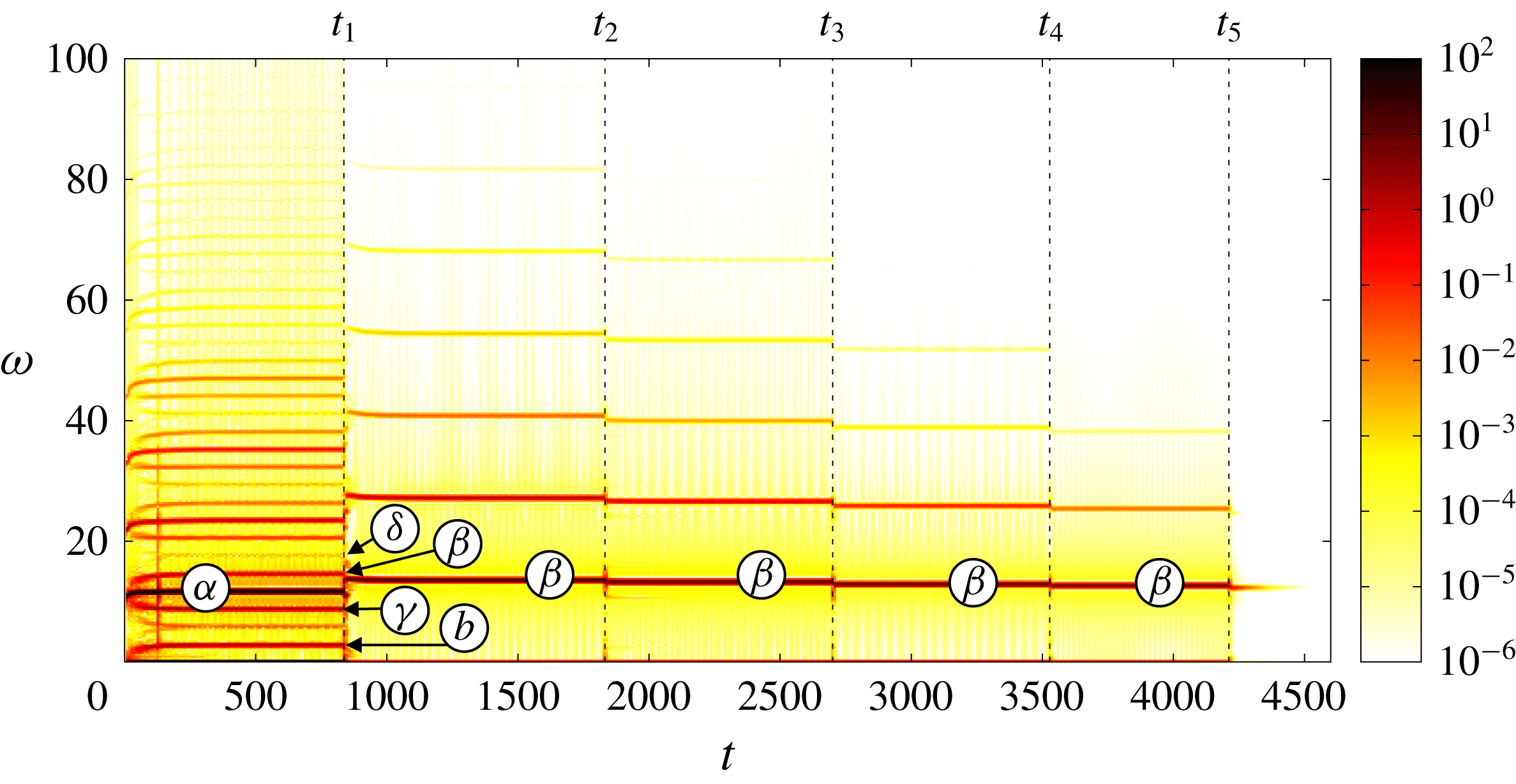
Spectrogram of the time series
 $y(t)$
, using short-time Fourier analysis with Hamming windows of length
 $T=20$
and
 $50\,\%$
overlap. In this section, we focus on the unforced flow for
 $t<t_{1}$
, but further comments regarding the controlled flow are provided in § 5.2. Resonant mean-flow modes
 $\unicode[STIX]{x1D6FC},\unicode[STIX]{x1D6FD},\unicode[STIX]{x1D6FE},\unicode[STIX]{x1D6FF}$
and
 $b$
are indicated, according to modal analysis reported in §§ 3.5 and 5.3. The start-up time
 $t_{m}$
of each controller correction
 $K_{m}^{\prime }$
is shown with a dashed line.

Recall that the base flow was initially perturbed with a ‘drop’ of the leading eigenmode, i.e. that of largest temporal growth rate. This shear-layer mode initially has a natural frequency of
 $\unicode[STIX]{x1D714}=10.9$
(Barbagallo et al.
Reference Barbagallo, Sipp and Schmid2009), as can be verified from the spectrogram in figure 8 (the part of the figure for
 $t>t_{1}$
will be discussed later in § 5.2). As the instability develops, the frequency shifts to higher values, reaching a value of
 $11.74$
when the flow is fully developed. We use this value to define a high-frequency scale
 $\unicode[STIX]{x1D714}_{h}$
associated with shear-layer oscillations. During the transient, we also observe the development of a low-frequency peak at
 $\unicode[STIX]{x1D714}_{l}\approx 2.89$
. The flow structures associated with
 $\unicode[STIX]{x1D714}_{l}$
and
 $\unicode[STIX]{x1D714}_{h}$
are shown in figure 9(a,b). Panel (b) confirms that the Koopman mode at
 $\unicode[STIX]{x1D714}_{h}$
is associated with a shear-layer mode. On the other hand, the low-frequency mode in (a) is localized within the cavity. The frequency is low because the recirculating mean flow within the cavity is slow. The two ‘fundamental’ frequencies
 $\unicode[STIX]{x1D714}_{h}$
and
 $\unicode[STIX]{x1D714}_{l}$
give rise to harmonics and interaction peaks visible in the spectrogram and the spectrum of state 0 in figure 7(a).
Comparison between real part of streamwise velocity component of Koopman modes at (a)
 $\unicode[STIX]{x1D714}=\unicode[STIX]{x1D714}_{l}$
, (b)
 $\unicode[STIX]{x1D714}=\unicode[STIX]{x1D714}_{h}$
and eigenmodes (c)
 $b$
, (d)
 $\unicode[STIX]{x1D6FC}$
of the uncontrolled mean flow. Koopman modes
 $\hat{\boldsymbol{q}}^{\prime }$
were approximated using DFT on a time series of 4013 snapshots equally sampled over a total duration of
 $128.416$
time units. The complex amplitude of the mean-flow eigenmodes was tuned to minimize the
 $L_{2}$
-error with respect to the Koopman modes. The colour map spans from the minimum to the maximum value in each plot, so bounds can be compared between Koopman modes and eigenmodes.

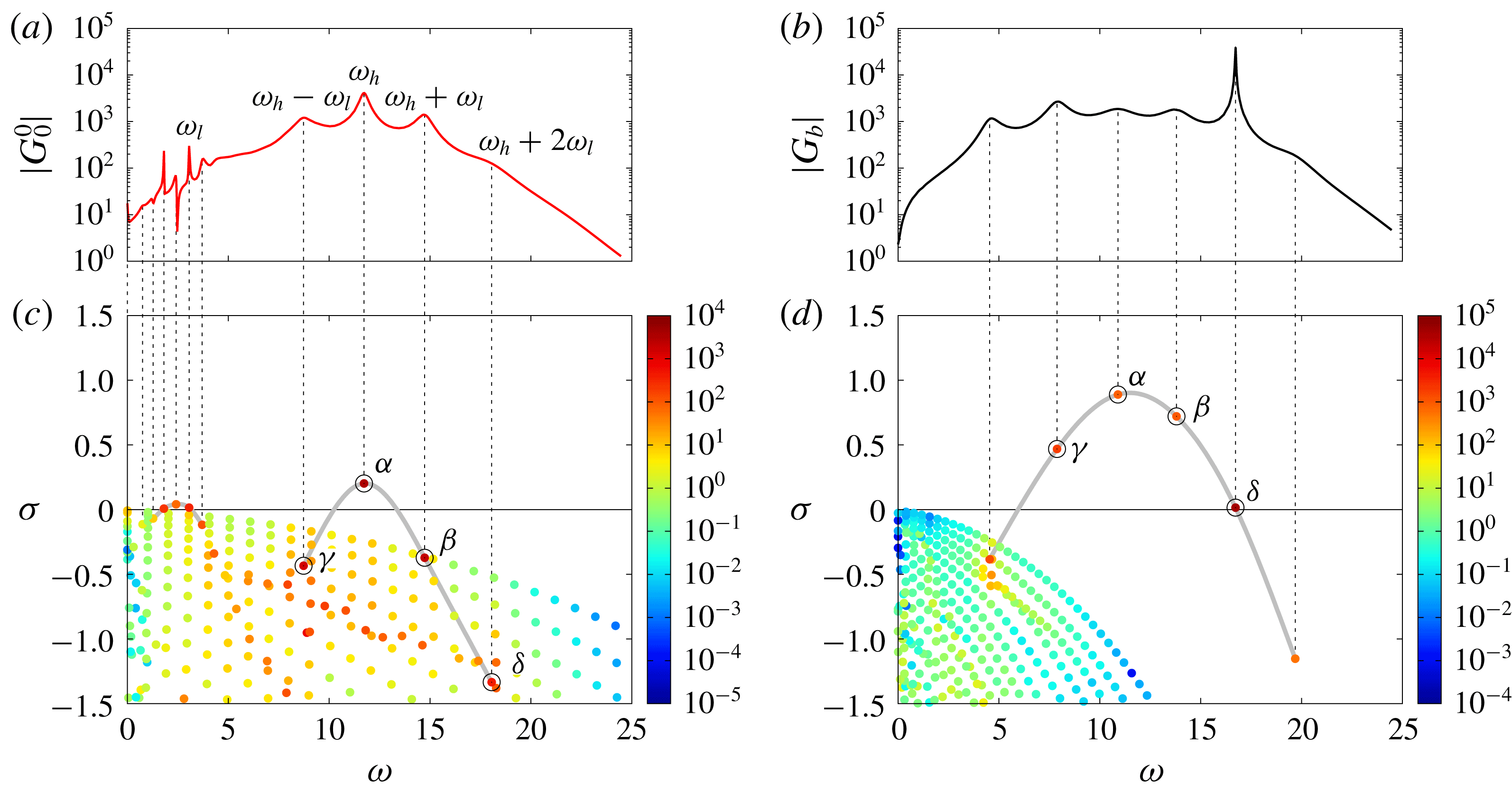
Frequency responses (a)
 $G_{0}^{0}$
and (b)
 $G_{b}$
of the mean and base flows, and corresponding sets of poles (c,d) calculated by modal analysis. Eigenvalues are coloured according to criterion (3.7) quantifying the relative contribution of each pole to the input–output relation. The (almost) one-to-one relation between resonance peaks and specific poles is highlighted with dashed vertical lines. These resonant poles can be grouped into a single family for the base flow, highlighted with a grey line in (d). This family contains the four unstable modes of the base flow, labelled with Greek characters
 $\unicode[STIX]{x1D6FC}$
,
 $\unicode[STIX]{x1D6FD}$
,
 $\unicode[STIX]{x1D6FE}$
and
 $\unicode[STIX]{x1D6FF}$
in decreasing order of growth rate and encircled in black. This family of resonant modes can also be identified, by continuity, in the mean-flow spectrum. A distinct family of modes
 $a$
–
 $f$
, also highlighted with a grey line in (c), is responsible for the low-frequency peaks present in
 $|G_{0}^{0}|$
.

3.5 Modal analysis
We illustrate in figure 10 the key property of our resolvent-based model explained in § 2.4, i.e. that eigenvalues of the mean flow
 $\overline{\boldsymbol{q}}_{0}$
correspond to poles of the transfer function
 $G_{0}^{0}$
, which can be related to instability modes of the base flow
 $\boldsymbol{q}_{b}$
. On the top panels, we plot the gain of the frequency response associated with the unforced mean flow
 $G_{0}^{0}(\text{i}\unicode[STIX]{x1D714})$
(a) and base flow
 $G_{b}(\text{i}\unicode[STIX]{x1D714})$
(b), the latter being defined as
 $$\begin{eqnarray}G_{b}:=\langle \boldsymbol{C},{\mathcal{R}}_{\boldsymbol{q}_{b}}\boldsymbol{B}\rangle .\end{eqnarray}$$
In both cases, we notice the presence of peaks indicating strong receptivity to external forcing on a discrete set of frequencies. In the case of (a), these peaks correspond to the frequencies of the Koopman modes. Hence, the unforced flow is most receptive to external forcing at its intrinsic oscillation frequencies, which is an indication that the mean-flow model captures relevant properties of the nonlinear system. The peaks of
 $G_{b}$
, on the other hand, do not match with nonlinear frequencies. In the two cases though, the peaks are associated with resonant poles of the respective model, corresponding to mean-flow or base-flow eigenvalues. We therefore plot the spectra of the associated Jacobian operators in (c,d), below the frequency responses. In order to identify which eigenvalues are responsible for the receptivity peaks, we colour the spectra by the criterion
 $$\begin{eqnarray}\unicode[STIX]{x1D6E4}_{j}={\displaystyle \frac{|\langle \boldsymbol{C},\boldsymbol{q}_{j}^{\prime }\rangle ||\langle \boldsymbol{p}_{j}^{\prime },\boldsymbol{B}\rangle |}{|\unicode[STIX]{x1D70E}_{j}|}},\end{eqnarray}$$
quantifying the contribution of each mode to the input–output relation (Antoulas Reference Antoulas2005; Bagheri et al.
Reference Bagheri, Brandt and Henningson2009; Barbagallo et al.
Reference Barbagallo, Sipp and Schmid2009). The criterion takes into account the distance
 $1/|\unicode[STIX]{x1D70E}_{l}|$
of each eigenvalue to the imaginary axis, the observability of the direct mode
 $|\langle \boldsymbol{C},\boldsymbol{q}_{l}^{\prime }\rangle |$
and the controllability of the adjoint mode
 $|\langle \boldsymbol{p}_{l}^{\prime },\boldsymbol{B}\rangle |$
. We recall that the adjoint modes
 $(\boldsymbol{p}_{l}^{\prime })$
are solutions of the eigenvalue problem
 $(\unicode[STIX]{x1D707}_{l}{\mathcal{B}}-\widetilde{{\mathcal{A}}}_{i}^{j}(\unicode[STIX]{x1D707}_{l}))\boldsymbol{p}_{l}^{\prime }=0$
, where
 $\widetilde{{\mathcal{A}}}_{i}^{j}$
is the adjoint of
 ${\mathcal{A}}_{i}^{j}$
with respect to the inner product (2.10). Eigenvalues of the adjoint operator are complex conjugate of the eigenvalues
 $(s_{l})$
of the direct operator, i.e.
 $\unicode[STIX]{x1D707}_{l}=s_{l}^{\ast }$
, and adjoint modes satisfy the biorthogonality relation
 $\langle \boldsymbol{p}_{k}^{\prime },\boldsymbol{q}_{l}^{\prime }\rangle =\unicode[STIX]{x1D6FF}_{kl}$
with the normalized direct modes
 $(\boldsymbol{q}_{l}^{\prime })$
. Using the criterion (3.7), we find two families of modes responsible for the resonance peaks of
 $G_{0}^{0}$
, and a single family of modes responsible for the peaks of
 $G_{b}$
. The modes are highlighted with grey lines in (c,d), intended to guide the eye. Four poles, labelled
 $\unicode[STIX]{x1D6FC}$
,
 $\unicode[STIX]{x1D6FD}$
,
 $\unicode[STIX]{x1D6FE}$
,
 $\unicode[STIX]{x1D6FF}$
are responsible for the peaks at
 $\unicode[STIX]{x1D714}>5$
in
 $G_{0}^{0}$
, corresponding to oscillations at
 $\unicode[STIX]{x1D714}_{h}$
,
 $\unicode[STIX]{x1D714}_{h}\pm \unicode[STIX]{x1D714}_{l}$
and
 $\unicode[STIX]{x1D714}_{h}+2\unicode[STIX]{x1D714}_{l}$
. The other family of mean-flow modes
 $a,b,c,d,e,f$
are responsible for the low-frequency peaks at
 $\unicode[STIX]{x1D714}<5$
, among which the peak at
 $\unicode[STIX]{x1D714}_{l}$
, coinciding with mode
 $b$
. The five resonance peaks of the base flow are generated by a single family of 5 poles. From the time–frequency analysis, we know that the high frequency
 $\unicode[STIX]{x1D714}_{h}$
is connected to the most unstable mode of the base flow. Therefore, mode
 $\unicode[STIX]{x1D6FC}$
is the mean-flow analogue of that specific base-flow eigenmode. The other mean-flow modes
 $\unicode[STIX]{x1D6FD}$
,
 $\unicode[STIX]{x1D6FE}$
,
 $\unicode[STIX]{x1D6FF}$
may then be identified with the remaining unstable modes of the base flow, hence the labelling in figure 10(c,d).
Conversely, the mean-flow mode
 $b$
responsible for the receptivity peak at
 $\unicode[STIX]{x1D714}_{l}$
in
 $G_{0}^{0}$
does not have an obvious base-flow analogue. In fact, the emergence of mode
 $b$
in the mean-flow spectrum seems to arise from a purely nonlinear mechanism comparable to ‘lock in’. Indeed, we notice that the frequency difference between each pair of modes within the set
 $\{\unicode[STIX]{x1D6FC},\unicode[STIX]{x1D6FD},\unicode[STIX]{x1D6FE},\unicode[STIX]{x1D6FF}\}$
is a multiple of the frequency
 $\unicode[STIX]{x1D714}_{l}$
associated with mode
 $b$
. Distortion of the base flow by the nonlinearities allows these four modes to synchronize with the low-frequency mode
 $b$
, resulting in a quasiperiodic attractor. A similar observation has already been made regarding low-frequency oscillations of large laminar separation bubbles behind a two-dimensional bump (Cherubini, Robinet & De Palma Reference Cherubini, Robinet and De Palma2010).
In figure 9, we compare the structure of the mean-flow eigenmodes
 $\unicode[STIX]{x1D6FC}$
and
 $b$
(c,d) with the Koopman modes of the unforced flow at
 $\unicode[STIX]{x1D714}_{h}$
and
 $\unicode[STIX]{x1D714}_{l}$
(a,b). We notice striking similarities between eigenmodes and Koopman modes, in line with observations from past studies recalled in the introduction. In the literature though, the success of mean-flow stability analysis is often associated with the presence of marginal eigenvalues (Turton et al.
Reference Turton, Tuckerman and Barkley2015; Mantič-Lugo & Gallaire Reference Mantič-Lugo and Gallaire2016), the so-called RZIF property (real-zero imaginary-frequency) in Turton et al. (Reference Turton, Tuckerman and Barkley2015). We highlight the fact that the RZIF property is not verified here: modes
 $b$
,
 $\unicode[STIX]{x1D6FC}$
,
 $\unicode[STIX]{x1D6FD}$
,
 $\unicode[STIX]{x1D6FE}$
and
 $\unicode[STIX]{x1D6FF}$
have non-zero, positive growth rates, yet they are associated with the correct frequencies and Koopman modes. This was already noticed by Mettot, Renac & Sipp (Reference Mettot, Renac and Sipp2014a
) and Meliga (Reference Meliga2017) in open-cavity flows (although in the former paper the mean flow was obtained as a fixed point of a RANS model, not a temporal average of an unsteady RANS simulation). Here, the approximation works because the mean flow yields an excellent approximation of the full flow at any instant (Mezić Reference Mezić2013), as previously said in § 3.4.
Finally, we observe in figure 10 receptivity peaks at low frequencies different from
 $\unicode[STIX]{x1D714}_{l}$
, due to the presence of poles
 $c$
,
 $a$
and
 $f$
close to the imaginary axis. The corresponding eigenmodes are localized within the cavity and resemble mode
 $b$
. Despite strong receptivity to external forcing, there is no signature of the associated frequencies in the spectrum of the unforced flow. To understand this, we need to consider the endogenous forcing term
 $$\begin{eqnarray}\boldsymbol{f}^{\prime }:=\unicode[STIX]{x1D6F9}_{\overline{\boldsymbol{q}}}\boldsymbol{q}^{\prime }\end{eqnarray}$$
due to the nonlinear feedback operator. Since the operator
 $\unicode[STIX]{x1D6F9}_{\overline{\boldsymbol{q}}}$
is time invariant, its output
 $\boldsymbol{f}^{\prime }$
is quasiperiodic with the same discrete set of frequencies as its input
 $\boldsymbol{q}^{\prime }$
, i.e.
 $\{\unicode[STIX]{x1D714}_{\boldsymbol{k}}\}$
defined in (3.5). More precisely, we can introduce the sets of Koopman modes
 $$\begin{eqnarray}\{\hat{\boldsymbol{q}}_{\boldsymbol{k}}^{\prime }\}:=\{\hat{\boldsymbol{q}}^{\prime }(\unicode[STIX]{x1D714}_{\boldsymbol{ k}})\},\quad \{\hat{\boldsymbol{f}}_{\boldsymbol{k}}^{\prime }\}:=\{\hat{\boldsymbol{f}}^{\prime }(\unicode[STIX]{x1D714}_{\boldsymbol{ k}})\}\end{eqnarray}$$
respectively associated with
 $\boldsymbol{q}^{\prime }$
and
 $\boldsymbol{f}^{\prime }$
. In the fully developed regime, the governing equations (2.2) can be recast in the form of a harmonic balance relation (Khalil Reference Khalil2002)
 $$\begin{eqnarray}\hat{\boldsymbol{q}}_{\boldsymbol{k}}^{\prime }={\mathcal{R}}_{\overline{\boldsymbol{q}}}(\text{i}\unicode[STIX]{x1D714}_{\boldsymbol{ k}})\hat{\boldsymbol{f}}_{\boldsymbol{k}}^{\prime },\end{eqnarray}$$
between these two sets of Koopman modes (harmonic averages are zero otherwise). Clearly, strong receptivity at frequencies outside the set
 $\{\unicode[STIX]{x1D714}_{\boldsymbol{k}}\}$
has no impact on the intrinsic dynamics because the endogenous forcings are zero at these frequencies. In short, the resolvent operator displays strong receptivity to external forcing at the natural oscillation frequencies of the unforced flow, but not exclusively.
4 Designing controller
$K_{1}^{\prime }$

We explain here the methodology used to synthesize controller
 $K_{1}^{\prime }$
, but all subsequent controller corrections are designed using the same methodology. There are two consecutive steps: first model reduction from frequency-domain data
 $G_{0}^{0}(\text{i}\unicode[STIX]{x1D714})$
, then structured
 ${\mathcal{H}}_{\infty }$
-synthesis using the ROM.
4.1 Model reduction
We convert the frequency response
 $G_{0}^{0}$
in the form of a state-space model
 $(\widetilde{\boldsymbol{A}},\widetilde{\boldsymbol{B}},\widetilde{\boldsymbol{C}},\widetilde{\boldsymbol{D}})$
. Although many points
 $O(100)$
are typically needed to capture the fine details of the frequency response, we seek a state-space model approximating
 $G_{0}^{0}$
with a lower order
 $O(10)$
to focus on the essential characteristics of the system that we would like to manipulate. A strictly proper (i.e.
 $\widetilde{\boldsymbol{D}}=0$
) reduced-order model (ROM) of order 16 is obtained using subspace identification methods (Liu, Jacques & Miller Reference Liu, Jacques and Miller1996; McKelvey, Akcay & Ljung Reference McKelvey, Akcay and Ljung1996). For subsequent iterations, the order of the ROM varies between 16 and 32. The frequency response of the ROM is given by
 $$\begin{eqnarray}\widetilde{G}_{0}^{0}(\text{i}\unicode[STIX]{x1D714})=\widetilde{\boldsymbol{C}}(\text{i}\unicode[STIX]{x1D714}\boldsymbol{I}-\widetilde{\boldsymbol{A}})^{-1}\widetilde{\boldsymbol{B}}\end{eqnarray}$$
and the associated poles correspond to eigenvalues of
 $\widetilde{\boldsymbol{A}}$
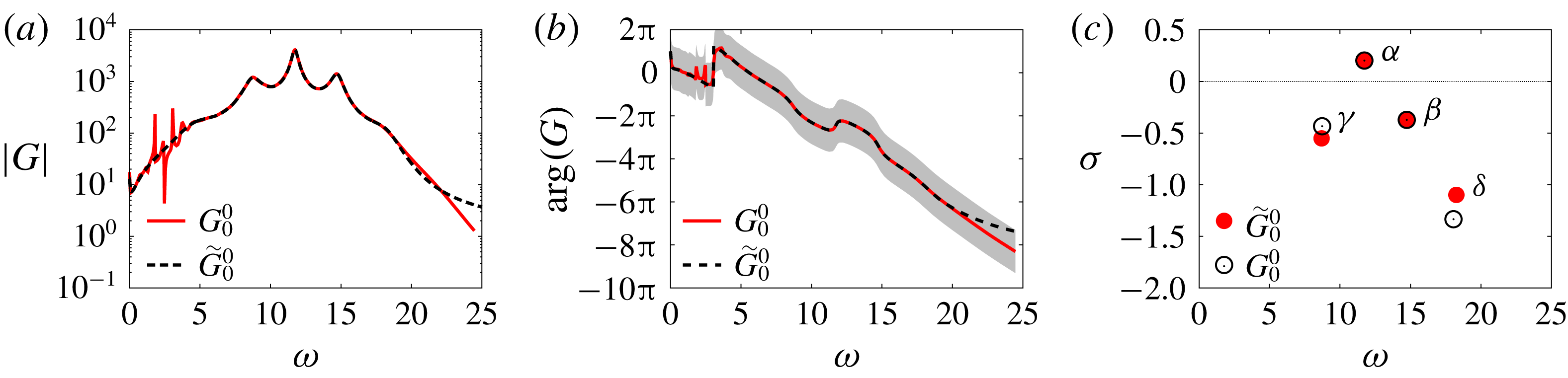
. In general, all quantities related to ROMs will be denoted with a tilde. In figure 11(a,b), we check that the frequency response
 $\widetilde{G}_{0}^{0}(\text{i}\unicode[STIX]{x1D714})$
(black dotted curve) coincides with the original model
 $G_{0}^{0}$
(solid red curve) over the frequency range
 $5<\unicode[STIX]{x1D714}<20$
. This range contains the main resonance peaks at
 $\unicode[STIX]{x1D714}_{h}$
,
 $\unicode[STIX]{x1D714}_{h}\pm \unicode[STIX]{x1D714}_{l}$
and
 $\unicode[STIX]{x1D714}_{h}+2\unicode[STIX]{x1D714}_{l}$
, but not the low-frequency ones at
 $\unicode[STIX]{x1D714}<5$
which we choose to ignore in order to ensure sufficient order reduction. In (c), we check that the poles
 $\unicode[STIX]{x1D6FC}$
,
 $\unicode[STIX]{x1D6FD}$
,
 $\unicode[STIX]{x1D6FE}$
and
 $\unicode[STIX]{x1D6FF}$
corresponding to the main resonance peaks are correctly approximated by some eigenvalues of
 $\widetilde{\boldsymbol{A}}$
.
Comparison between resolvent-based model
 $G_{0}^{0}$
(solid red line/solid symbols) and the ROM
 $\widetilde{G}_{0}^{0}$
(dashed black line/open symbols) obtained by subspace identification: frequency response (a) gain and (b) phase (the shaded region corresponds to
 $|\text{arg}(G)-\text{arg}(G_{0}^{0})|\leqslant \unicode[STIX]{x03C0}$
); (c) poles
 $\unicode[STIX]{x1D6FC},\unicode[STIX]{x1D6FD},\unicode[STIX]{x1D6FE},\unicode[STIX]{x1D6FF}$
.
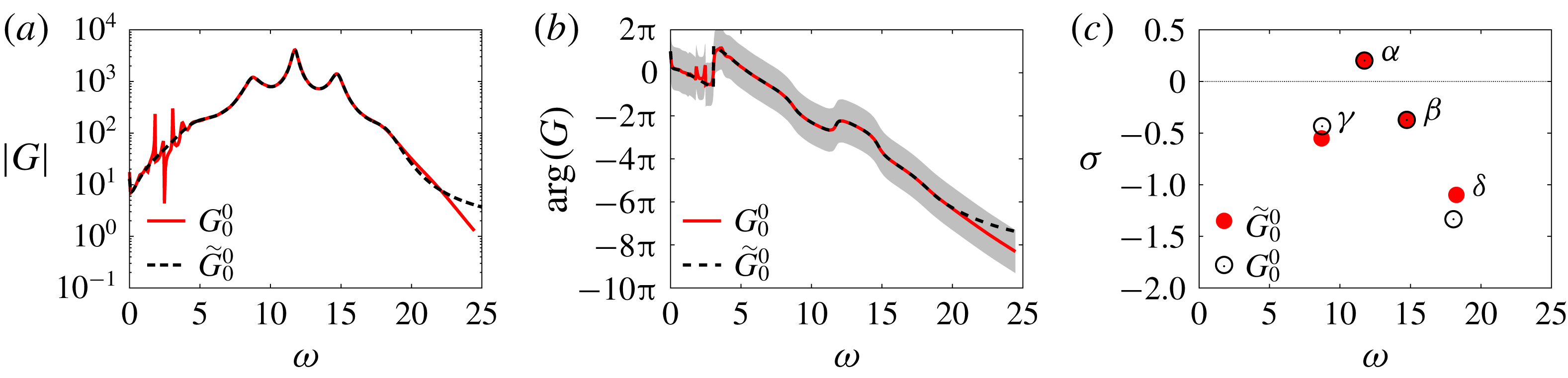
We note in passing the monotonically decreasing phase (except for ‘upward jumps’ corresponding to unstable modes) with a nearly constant negative slope in (b), which characterizes a time delay between the actuator and the sensor. This time delay corresponds to advection of the perturbations over the cavity of length
 $L=1$
at the mean velocity
 $\unicode[STIX]{x1D705}U$
in the shear layer. Fitting the data with a straight line in the range
 $5\leqslant \unicode[STIX]{x1D714}\leqslant 25$
leads to a value of
 $\unicode[STIX]{x1D705}\approx 0.73$
, consistent with the mean flow in figure 6(a). This value of
 $\unicode[STIX]{x1D705}$
is larger than the value 0.53 obtained by Barbagallo et al. (Reference Barbagallo, Sipp and Schmid2009) for the advection of pressure perturbations by the base flow at
 $x_{2}=0$
above the cavity. This difference is mainly due to the fact that the forcing field
 $\boldsymbol{B}$
is localized within the incoming boundary layer at
 $x_{2}^{0}=0.02>0$
and not directly at the wall.
4.2 Structured
${\mathcal{H}}_{\infty }$
-synthesis

After designing a ROM, we seek a controller
 $K_{1}^{\prime }$
outputting the forcing signal
 $$\begin{eqnarray}u_{1}^{\prime }:=K_{1}^{\prime }y\end{eqnarray}$$
from the measurement
 $y$
. When the plant
 $\widetilde{G}_{0}^{0}$
is interconnected with
 $K_{1}^{\prime }$
, the closed loop is characterized by four transfer functions
 $$\begin{eqnarray}\left[\begin{array}{@{}c@{}}y\\ u_{1}^{\prime }\end{array}\right]=\left[\begin{array}{@{}cc@{}}\widetilde{G}_{0}^{0}S & S\\ T & K_{1}^{\prime }S\end{array}\right]\left[\begin{array}{@{}c@{}}n\\ w\end{array}\right],\end{eqnarray}$$
linking the two inputs
 $n$
and
 $w$
to the two outputs
 $y$
and
 $u_{1}^{\prime }$
. These four transfers are combinations of only two interconnected blocks
 $\widetilde{G}_{0}^{0}$
and
 $K_{1}^{\prime }$
, therefore they are not independent of each other. In particular, the sensitivity function
 $S$
and complementary sensitivity function
 $T$
, respectively defined as
 $$\begin{eqnarray}S={\displaystyle \frac{1}{1-\widetilde{G}_{0}^{0}K_{1}^{\prime }}}\quad \text{and}\quad T={\displaystyle \frac{\widetilde{G}_{0}^{0}K_{1}^{\prime }}{1-\widetilde{G}_{0}^{0}K_{1}^{\prime }}},\end{eqnarray}$$
satisfy the relation
 $S-T=1$
. The controller
 $K_{1}^{\prime }$
is designed in order to achieve desired specifications on the four closed-loop transfer functions. But because the four transfer functions are not independent of each other, we can only constrain each of them in a limited frequency range. Four filters
 $W_{S},W_{T},W_{GS},W_{K^{\prime }S}$
are therefore designed in order to shape each closed-loop transfer function adequately and achieve specific design goals to be listed in the next subsections. The procedure amounts to minimizing a positive constant
 $\unicode[STIX]{x1D70C}$
bounding the
 ${\mathcal{H}}_{\infty }$
-norm of the four weighted transfer functions
 $$\begin{eqnarray}\displaystyle & \displaystyle \Vert W_{S}S\Vert _{\infty }\leqslant \unicode[STIX]{x1D70C}, & \displaystyle\end{eqnarray}$$
 $$\begin{eqnarray}\displaystyle & \displaystyle \Vert W_{T}T\Vert _{\infty }\leqslant \unicode[STIX]{x1D70C}, & \displaystyle\end{eqnarray}$$
 $$\begin{eqnarray}\displaystyle & \displaystyle \Vert W_{GS}\widetilde{G}_{0}^{0}S\Vert _{\infty }\leqslant \unicode[STIX]{x1D70C}, & \displaystyle\end{eqnarray}$$
 $$\begin{eqnarray}\displaystyle & \displaystyle \Vert W_{K^{\prime }S}K_{1}^{\prime }S\Vert _{\infty }\leqslant \unicode[STIX]{x1D70C}, & \displaystyle\end{eqnarray}$$
while simultaneously ensuring that the closed-loop transfers and the controller
 $K_{1}^{\prime }$
remain stable. We recall that for a single-input single-output (SISO) system, the
 ${\mathcal{H}}_{\infty }$
-norm of a stable transfer function
 $H$
is given by the maximum of the modulus of the frequency response
 $$\begin{eqnarray}\Vert H\Vert _{\infty }=\max _{\unicode[STIX]{x1D714}\in \mathbb{R}}|H(\text{i}\unicode[STIX]{x1D714})|,\end{eqnarray}$$
hence, conditions (4.5)–(4.8) are equivalent to
 $$\begin{eqnarray}\displaystyle & \displaystyle |S(\text{i}\unicode[STIX]{x1D714})|\leqslant \unicode[STIX]{x1D70C}/|W_{S}(\text{i}\unicode[STIX]{x1D714})|, & \displaystyle\end{eqnarray}$$
 $$\begin{eqnarray}\displaystyle & \displaystyle |T(\text{i}\unicode[STIX]{x1D714})|\leqslant \unicode[STIX]{x1D70C}/|W_{T}(\text{i}\unicode[STIX]{x1D714})|, & \displaystyle\end{eqnarray}$$
 $$\begin{eqnarray}\displaystyle & \displaystyle |\widetilde{G}_{0}^{0}S(\text{i}\unicode[STIX]{x1D714})|\leqslant \unicode[STIX]{x1D70C}/|W_{GS}(\text{i}\unicode[STIX]{x1D714})|, & \displaystyle\end{eqnarray}$$
 $$\begin{eqnarray}\displaystyle & \displaystyle |K_{1}^{\prime }S(\text{i}\unicode[STIX]{x1D714})|\leqslant \unicode[STIX]{x1D70C}/|W_{KS}(\text{i}\unicode[STIX]{x1D714})|, & \displaystyle\end{eqnarray}$$
for all real values of
 $\unicode[STIX]{x1D714}$
. The design of controller
 $K_{1}^{\prime }$
therefore rests on the definition of four inequality constraints on the closed-loop transfer functions. The constraints are enforced by designing well-chosen frequency-domain templates
 $1/W_{S}$
,
 $1/W_{T}$
,
 $1/W_{GS}$
and
 $1/W_{KS}$
. These are defined as filters depending on free parameters which are calibrated manually before
 $\unicode[STIX]{x1D70C}$
is minimized. If one of the closed-loop constraints is not met, the free parameters are adjusted and
 $\unicode[STIX]{x1D70C}$
optimized again, in an iterative fashion until all constraints are satisfied.
The present approach targets the shaping of all four closed-loop transfer functions and differs from the mixed-sensitivity method, which only targets
 $S$
,
 $T$
and sometimes
 $K_{1}^{\prime }S$
(Henning & King Reference Henning and King2007; Henning et al.
Reference Henning, Pastoor, King, Noack, Tadmor and King2007; Williams et al.
Reference Williams, Kerstens, Pfeiffer, King and Colonius2010), but not
 $\widetilde{G}_{0}^{0}S$
. The advantage of the four-block method over mixed sensitivity will become clear in § 4.2.1. We note that directly shaping the closed-loop transfer functions is a much more challenging task than shaping the loop gain
 $\widetilde{G}_{0}^{0}K_{1}^{\prime }$
, as done in the loop-shaping approach (Dahan et al.
Reference Dahan, Morgans and Lardeau2012; Jones et al.
Reference Jones, Heins, Kerrigan, Morrison and Sharma2015; Li & Morgans Reference Li and Morgans2016; Dalla Longa et al.
Reference Dalla Longa, Morgans and Dahan2017). Loop shaping takes advantage of the linearity of the loop gain with respect to the controller
 $K_{1}^{\prime }$
in order to indirectly achieve constraints on the closed loop at low cost, whereas both the mixed-sensitivity and the four-block frameworks target the closed loop in a more direct fashion.
Here we use a structured
 ${\mathcal{H}}_{\infty }$
framework, which means that the controller order may be chosen a priori, i.e. independently of the order of the ROM. In our case, we fix the order of
 $K_{1}^{\prime }$
and all subsequent controller corrections to 10. This is another key difference with the loop-shaping approach, where the order of the controller cannot be chosen freely and is always larger than that of the ROM. However, computing fixed-order controllers for the
 ${\mathcal{H}}_{\infty }$
-synthesis problem is known to be NP-hard (Blondel & Tsitsiklis Reference Blondel and Tsitsiklis1997) and one has to rely on local optimization techniques to compute simple and practical controllers. In this work, we have used the control software hinfstruct from the MATLAB Control Toolbox, which is based on a non-convex non-smooth bundle technique developed in Apkarian & Noll (Reference Apkarian and Noll2006).
In the rest of this section, we will explain the specifications on the closed-loop transfer functions and the choice of appropriate frequency templates. The final transfer functions (black lines) and frequency templates (blue lines) are shown in figure 12, before (solid) and after (dashed) optimization of the parameter
 $\unicode[STIX]{x1D70C}$
to a final value of 0.6.
Frequency response of the four closed-loop transfer functions of the ROM (black lines): (a)
 $\widetilde{G}_{0}^{0}S$
, (b)
 $S$
, (c)
 $T$
, (d)
 $K_{1}^{\prime }S$
. The frequency templates
 $\unicode[STIX]{x1D70C}/|W_{GS}|$
,
 $\unicode[STIX]{x1D70C}/|W_{S}|$
,
 $\unicode[STIX]{x1D70C}/|W_{T}|$
are plotted in blue (
 $\unicode[STIX]{x1D70C}/|W_{K^{\prime }S}|$
is not shown in (d) as it is just a constant curve located well above the maximum of
 $|K_{1}^{\prime }S|$
), with solid lines for
 $\unicode[STIX]{x1D70C}=1$
and dashed lines for the optimized value of the multiplicative constant
 $\unicode[STIX]{x1D70C}=0.6$
. In (b), the shaded region is the forbidden area where the modulus margin constraint (4.20) is violated.

4.2.1 Shaping
$\widetilde{G}_{0}^{0}S$
: attenuation of the main resonance peak

The goal of the controller is to suppress intrinsic resonances. To ‘desensitize’ the flow to input perturbations
 $n$
at the main resonance frequency
 $\unicode[STIX]{x1D714}=\unicode[STIX]{x1D714}_{h}$
of
 $G_{0}^{0}(\text{i}\unicode[STIX]{x1D714})$
, we must ensure that
 $$\begin{eqnarray}|S(\text{i}\unicode[STIX]{x1D714}_{h})|<1,\end{eqnarray}$$
such that the closed-loop gain
 $$\begin{eqnarray}|\widetilde{G}_{0}^{1}|=|\widetilde{G}_{0}^{0}S|\end{eqnarray}$$
be smaller than the open-loop gain
 $|\widetilde{G}_{0}^{0}|$
at this frequency. This is achieved by designing a ‘bell-shaped’ frequency template
 $$\begin{eqnarray}1/W_{GS}=1/k_{GS}{\displaystyle \frac{s^{2}/\unicode[STIX]{x1D6FC}^{2}+2\unicode[STIX]{x1D709}\unicode[STIX]{x1D714}_{h}s+\unicode[STIX]{x1D714}_{h}^{2}/\unicode[STIX]{x1D6FC}^{2}}{s^{2}+2\unicode[STIX]{x1D709}\unicode[STIX]{x1D714}_{h}s+\unicode[STIX]{x1D714}_{h}^{2}}},\end{eqnarray}$$
with
 $\unicode[STIX]{x1D6FC}^{2}>1$
(see figure 12
a) applied to the closed-loop transfer function
 $\widetilde{G}_{0}^{0}S$
. The gain
 $|1/W_{GS}(\text{i}\unicode[STIX]{x1D714})|$
varies between a minimum value of
 $1/(\unicode[STIX]{x1D6FC}^{2}k_{GS})$
, reached asymptotically when
 $\unicode[STIX]{x1D714}\rightarrow 0$
and
 $\unicode[STIX]{x1D714}\rightarrow \infty$
, and a maximum value of
 $1/k_{GS}$
, reached at the resonance frequency
 $\unicode[STIX]{x1D714}=\unicode[STIX]{x1D714}_{h}$
. The parameter
 $\unicode[STIX]{x1D709}$
determines the width of the filter. By choosing
 $$\begin{eqnarray}k_{GS}=1/|\widetilde{G}_{0}^{0}(\text{i}\unicode[STIX]{x1D714}_{h})|\end{eqnarray}$$
and constraining
 $\widetilde{G}_{0}^{0}S$
, we indirectly enforce a constraint on the sensitivity function
 $$\begin{eqnarray}|S(\text{i}\unicode[STIX]{x1D714}_{h})|<\unicode[STIX]{x1D70C}.\end{eqnarray}$$
Since the optimal value of
 $\unicode[STIX]{x1D70C}$
is 0.6 in our case, we enforce a reduction of
 $60\,\%$
in the height of the main resonance peak at
 $\unicode[STIX]{x1D714}_{h}$
.
Shaping
 $\widetilde{G}_{0}^{0}S$
in order to constrain
 $S$
may seem counterintuitive at first sight: why not directly shaping
 $S$
? The aim of this ‘trick’ is to prevent pole cancellation by a zero of the controller. Indeed, cancelling the pole
 $\unicode[STIX]{x1D6FC}$
with a zero of
 $K_{1}^{\prime }$
is not a robust way to suppress the resonance at
 $\unicode[STIX]{x1D714}_{h}$
since the mean-flow model is only an approximation of the true plant. Worse still, the unstable pole
 $\unicode[STIX]{x1D6FC}$
will remain present in the closed loop through the transfer
 $\widetilde{G}_{0}^{0}S$
. A much better alternative is to strongly damp the growth rate associated with this pole by shaping
 $\widetilde{G}_{0}^{0}S$
instead of
 $S$
. When targeting the sensitivity function, as in the mixed-sensitivity approach, pole cancellation would typically occur since
 $S$
is a function of the product
 $\widetilde{G}_{0}^{0}K_{1}^{\prime }$
, i.e. the loop gain, only. The same problem occurs in the loop-shaping framework, which directly targets the loop gain. When targeting
 $\widetilde{G}_{0}^{0}S$
instead, pole cancellation does not occur since that transfer depends on both the loop gain and
 $\widetilde{G}_{0}^{0}$
. The four-block approach is therefore well suited to the control of unstable plants.
In fact, with appropriate choices for
 $\unicode[STIX]{x1D6FC}$
and
 $\unicode[STIX]{x1D709}$
, we see in figure 12(a) that we manage to suppress all three resonance peaks at
 $\unicode[STIX]{x1D714}_{h}$
and
 $\unicode[STIX]{x1D714}_{h}\pm \unicode[STIX]{x1D714}_{l}$
, associated with modes
 $\unicode[STIX]{x1D6FC}$
,
 $\unicode[STIX]{x1D6FD}$
and
 $\unicode[STIX]{x1D6FE}$
. As a result, we verify in (b) that the gain of the sensitivity function is less than 1 at these three frequencies. We also verify in this panel that
 $\unicode[STIX]{x1D70C}=|S(\text{i}\unicode[STIX]{x1D714}_{h})|=0.6$
. We will later verify in figure 17 from § 5.3 that the corresponding poles
 $\unicode[STIX]{x1D6FC}$
,
 $\unicode[STIX]{x1D6FD}$
and
 $\unicode[STIX]{x1D6FE}$
are indeed damped instead of being cancelled.
4.2.2 Shaping
$S$
: stability robustness (modulus margin)

The poles of all four closed-loop transfer functions are given by the zeros of
 $1-\widetilde{G}_{0}^{0}K_{1}^{\prime }$
. To ensure closed-loop stability, we must therefore ensure that all zeros lie in the appropriate half-plane. To guarantee stability robustness, we also ask that these zeros be sufficiently far from the imaginary axis, where the closed loop becomes marginally stable. Equivalently, for a stable closed loop, we may ask that the modulus margin (not to be confused with the gain margin)
 $$\begin{eqnarray}\unicode[STIX]{x0394}M=\min _{\unicode[STIX]{x1D714}\in \mathbb{R}}|1-\widetilde{G}_{0}^{0}(\text{i}\unicode[STIX]{x1D714})K_{1}^{\prime }(\text{i}\unicode[STIX]{x1D714})|\end{eqnarray}$$
be sufficiently large. In practice, we ask that
 $\unicode[STIX]{x0394}M>-6$
dB, or
 $\unicode[STIX]{x0394}M>0.5$
in linear scale, which amounts to bounding the sensitivity function
 $$\begin{eqnarray}\Vert S\Vert _{\infty }<2.\end{eqnarray}$$
The constraint on
 $S(\text{i}\unicode[STIX]{x1D714})$
being independent of
 $\unicode[STIX]{x1D714}$
, we consider a constant frequency template
 $1/W_{S}$
and optimize
 $\unicode[STIX]{x1D70C}$
such that
 $$\begin{eqnarray}|S(\text{i}\unicode[STIX]{x1D714})|\leqslant {\displaystyle \frac{\unicode[STIX]{x1D70C}}{|W_{S}|}}<2\end{eqnarray}$$
for any real
 $\unicode[STIX]{x1D714}$
. In figure 12(b), constraint (4.20) is represented by the shaded region. We see that the value of
 $\unicode[STIX]{x1D70C}=0.6$
reached after optimization did not allow the constraint to be satisfied in the vicinity of
 $\unicode[STIX]{x1D714}\approx 13$
, with the chosen
 $W_{S}$
. However, the sensitivity gain being almost equal to 2 there, the resulting controller is deemed satisfactory without further changing
 $W_{S}$
.
4.2.3 Shaping
$T$
: enforcing zero controller static gain

To ensure that the base flow is the only fixed point of the closed loop, we need to ensure the controller has zero static gain, as discussed in § 2.3. Imposing (2.30), i.e.
 $K_{1}^{\prime }(0)=0$
, is equivalent to a condition on the complementary sensitivity function
 $$\begin{eqnarray}T(0)=0,\end{eqnarray}$$
which can be approximately achieved using constraint (4.11) and a filter
 $W_{T}$
with a sufficiently large static gain
 $|W_{T}(0)|\gg 1$
, such that
 $$\begin{eqnarray}|T(0)|<{\displaystyle \frac{\unicode[STIX]{x1D70C}}{|W_{T}(0)|}}\ll 1.\end{eqnarray}$$
The frequency template
 $1/W_{T}$
is therefore defined as a high-pass filter, as can be verified in figure 12(c).
4.2.4 Shaping
$K_{1}^{\prime }S$
: performance robustness to modelling errors at high frequency

Finally, the remaining transfer function
 $K_{1}^{\prime }S$
may be shaped in order to ‘desensitize’ the controller at high frequency. This can be useful if modelling errors are large at high frequencies and if the signal
 $y$
is stochastic or contaminated with noise. This would typically be the case in an amplifier flow or in the context of turbulence. To achieve sufficient ‘roll-off’ of the controller gain at high frequency, a low-pass frequency template
 $1/W_{K^{\prime }S}$
may be used. In our case, we expect our model to become inaccurate at large frequencies since the resolvent operator about the mean flow only captures spatially coherent structures typically developing at low to moderate frequencies. However, our signal
 $y$
being deterministic, non-chaotic, noise free and therefore weakly energetic at high frequencies (cf. spectrum in figure 7
a), imposing steep roll-off at high frequency is unnecessary. We therefore choose
 $1/W_{K^{\prime }S}$
as a very large constant here, and simply verify a posteriori in figure 12(d) that the obtained controller is strictly proper, i.e. that
 $|K_{1}^{\prime }(\text{i}\unicode[STIX]{x1D714})|\rightarrow 0$
as
 $\unicode[STIX]{x1D714}\rightarrow \infty$
.
5 Controlled flow
Time series of (a) the perturbation kinetic energy
 $E$
, the sensor perturbation
 $y$
and the control signal
 $u=\sum _{m}u_{m}^{\prime }$
for the controlled flow. The time axis is in log scale to highlight the different time scales. For each iteration
 $m$
, the time origin is reset to zero by subtracting
 $t_{m}$
, the start-up time of the new controller
 $K_{m}^{\prime }$
, so that the first point is at
 $\text{d}t=4\times 10^{-4}$
in each panel.

5.1 Time scales
A sequence of five robust controllers was found to lead the flow from state 0 to the base flow. When a controller correction
 $K_{m}^{\prime }$
is added to the loop, its internal state is initialized to 0. The internal states of the other controllers
 $K_{j<m}^{\prime }$
already in the loop are not reset to 0, hence the control signal
 $u$
evolves continuously over time. Figure 13 shows the full time evolution of the system as the sequence of controllers is applied. In this plot, we concentrate on the transient evolution from one state to the next. The origin of time is reset to zero at each iteration
 $m$
, by subtracting the start-up time
 $t_{m}$
of a new controller
 $K_{m}^{\prime }$
. The time axis is in log scale, and different shades of grey are used to highlight the different time scales involved in the journey of the system from one state to the next. When a new controller is switched on, the flow rapidly evolves over a short time scale of the order of
 $O(1)$
, which seems sufficient for the system to latch onto a new state. This time scale is indicated with a white background. Subsequent evolution of the local measurement
 $y$
is insignificant, but the perturbation kinetic energy keeps evolving considerably over the next
 $O(100)$
time units. This slow relaxation is indicated with a light grey background, and a dark grey background is used to denote convergence to a new equilibrium. The separation of time scales in the transient evolution is once again related to the two physical processes occurring in the flow: fast oscillations of the shear layer and slow recirculation within the cavity. Indeed, due to its position, the local measurement
 $y$
is mostly sensitive to the former process and very little to the latter. Conversely, the global measurement
 $E$
is, by definition, sensitive to both. The control signal is characterized by a third, ultra-fast, time scale
 $O(0.1)$
, highlighted in very dark grey and visible at iteration 1 only. This time scale is intrinsic to the controller and the large ‘overshoot’ observed at the first iteration is due to the transition from a 2-torus to a limit cycle with a different fundamental frequency. Such qualitative transition does not occur in subsequent iterations, as we shall see next.
In the last iteration, all three quantities vanish as the system is attracted towards the base flow, which is a solution of the Navier–Stokes equation without forcing. At this point, the power consumption of the controllers is infinitesimal (or proportional to incoming noise in a realistic case) and the cavity drag is minimal, so the control strategy is profitable in the long run, regardless of the initial cost. The exponential decay of all quantities is governed by the least damped pole of the last transfer function
 $G_{5}^{5}$
.
5.2 Attractors
In figure 8 from § 3, we plotted a spectrogram of the time series
 $y(t)$
, which shows the evolution of the frequency content of the flow as it evolves. We comment here the part for
 $t>t_{1}$
concerning the controlled flow. We immediately notice in the spectrogram that there is less and less energy at high frequencies as we iterate, which indicates that the nonlinearity becomes weaker and weaker, before a linear regime is eventually reached at iteration 5. Initially, the dynamics is on a 2-torus characterized by the two fundamental frequencies
 $\unicode[STIX]{x1D714}_{l}$
and
 $\unicode[STIX]{x1D714}_{h}$
. But soon after
 $t_{1}$
, the flow transitions to a limit cycle with a fundamental frequency close to the previous harmonic
 $\unicode[STIX]{x1D714}_{h}+\unicode[STIX]{x1D714}_{l}$
. During subsequent iterations, the flow stays on (nearly) that same attractor, but the fundamental frequency slightly decreases. In fact, in the second iteration (between
 $t_{2}$
and
 $t_{3}$
), the attractor is not exactly a pure limit cycle but an almost degenerate 2-torus, which is strongly dominated by its fast fundamental frequency. The trace of interactions between the high-frequency fundamental and a non-zero low-frequency mode at
 $\unicode[STIX]{x1D714}\approx 2.5$
is visible soon after
 $t_{2}$
in figure 8.
Focussing on the permanent states in figure 13, we notice that each controller leads to a reduction of up to a decade in the perturbation kinetic energy (a). The decrease of the oscillation amplitude at the sensor
 $y$
is less dramatic (b). In figure 14, we project each attractor in the phase plane
 $[\unicode[STIX]{x0394}u_{2}(1/4,0),\unicode[STIX]{x0394}u_{2}(3/4,0)]$
. We observe a qualitative change in the topology of the attractor from state 0 (two-dimensional) to state 1 (one-dimensional). After that, each additional controller further reduces the amplitude of shear-layer oscillations, without further qualitative change in the dynamics.
Characterization of dynamical equilibria
 $m=0,\ldots ,5$
in the phase plane
 $[\unicode[STIX]{x0394}u_{2}(1/4,0),\unicode[STIX]{x0394}u_{2}(3/4,0)]$
. As the control law is updated, the end state moves closer and closer to the fixed point (state 5), which is located at
 $(0,0)$
. State 0 is a 2-torus, states 1–4 are limit cycles (or almost) with decreasing oscillation amplitude and state 5 is the fixed point. State 2 is in fact an almost degenerate 2-torus: the extra dimension of the attractor is so thin that it is hidden by the line width.

In figure 15, we also plot vorticity snapshots for each state, at a time of maximal shear stress
 $y$
. The reduction of the mean recirculation and the suppression of the low-frequency cavity mode are responsible for the strong weakening of the vorticity sheet within the cavity between states 0 and 1. The snapshots also illustrate the weakening of the spatial instability in the shear layer: roll up is delayed and the resulting vortices are therefore weaker as they impact the downstream edge of the cavity. We also notice a reduction in the size of the vortices between states 0 and 1, which is consistent with the increase in the oscillation frequency observed in figure 8.
Vorticity snapshots at a time where the shear-stress measurement
 $y$
is maximum (a)
 $m=0$
, (b)
 $m=1$
, (c)
 $m=2$
, (d)
 $m=3$
, (e)
 $m=4$
, (f)
 $m=5$
. The colour map has been cropped to the same arbitrary extremal values in all plots for comparison.

Evolution of the gain
 $|G|$
during the iterative procedure. (a) Shows the initial value of
 $|G|$
at the beginning of the iteration, at
 $t_{0}^{-}$
. In each subsequent panel, we show the relaxation of
 $G$
from
 $G_{m-1}^{m}$
(dashed lines) at
 $t=t_{m}^{+}$
to
 $G_{m}^{m}$
(solid lines) at
 $t=t_{m+1}^{-}$
(with
 $t_{6}\rightarrow \infty$
), under the effects of nonlinearity. Same labels as figure 15. Vertical lines indicate Koopman frequencies of the permanent state obtained with the controller
 $K_{m}$
(no unsteady peak for
 $m=5$
, because the system is steady). We also indicate which poles of
 $G_{m}^{m}$
are responsible for each receptivity peak. Mode labels are coloured when their receptivity peak matches with a Koopman frequency of the flow.

5.3 Evolution of the transfer function model
$G$
from
$n$
to
$y$
: gain and poles


In figure 16, we follow the evolution of the gain of the transfer function model
 $G$
characterizing the input–output relation from
 $n$
to
 $y$
, during the iteration. All mean flows were computed by averaging over more than 200 time units, in the fully developed regime. The plant
 $G_{m}^{m}$
(solid lines), computed using (2.32), characterizes the fully developed flow in feedback loop with the controller
 $K_{m}$
. At
 $t=t_{m+1}$
, a new controller correction
 $K_{m+1}^{\prime }$
is added to the loop, in order to desensitize the plant with respect to incoming perturbations occurring at resonant frequencies. As previously said in § 4.2.1, each controller targets the receptivity peaks matching with Koopman modes (indicated with solid lines), using a ‘bell-shaped’ filter (cf. (4.16)) centred about the dominant Koopman mode. This procedure leads to the shaped plant
 $G_{m}^{m+1}$
(dashed lines). The flow being out of equilibrium, it transiently evolves until a new dynamical state is reached. The new plant
 $G$
is then characterized by the transfer function
 $G_{m+1}^{m+1}$
(solid lines) and the iteration proceeds. In the last step, the flow state 4 is very close to the base flow already and the designed closed loop
 $G_{5}^{4}$
is therefore nearly equal to the last effective plant
 $G_{5}^{5}$
.
In figure 17, we plot the poles of each transfer function
 $G$
during the iteration. The poles of
 $G_{m}^{m}$
are indicated with solid symbols and those of the shaped plant
 $G_{m}^{m+1}$
are indicated with open symbols. In fact, the poles are computed from a ROM
 $\widetilde{G}$
obtained by subspace identification of
 $G$
, at each step. We only follow the evolution of the four poles
 $\unicode[STIX]{x1D6FC}$
,
 $\unicode[STIX]{x1D6FD}$
,
 $\unicode[STIX]{x1D6FE}$
,
 $\unicode[STIX]{x1D6FF}$
captured by the ROM. We checked in § 4.1 that the poles are well approximated in the case of
 $G_{0}^{0}$
(see figure 11
c). The plant
 $G_{m}^{m}$
always has unstable poles, until the very last iteration. During the ‘shaping’ phase (dashed arrows)
 $G_{m}^{m}\rightarrow G_{m}^{m+1}$
, the plant is stabilized. The growth rate of all four resonant poles is damped (except pole
 $\unicode[STIX]{x1D6FE}$
in the last iteration; panel (f)). Pushing the poles far from the imaginary axis attenuates the receptivity peaks in the transfer function, as observed in figure 16 and previously explained in § 4.2.1. The most strongly damped pole is associated with the frequency of the dominant Koopman mode, specifically targeted by the ‘bell-shaped’ template. Then, during the relaxation phase
 $G_{m}^{m+1}\rightarrow G_{m+1}^{m+1}$
, all the poles drift upwards again (solid arrows) and settle closer to the imaginary axis, causing the resurgence of sharp peaks in the next plant
 $G_{m+1}^{m+1}$
. In the last step, the flow is weakly nonlinear and the drift of the poles during the relaxation phase is sufficiently small for all of them to remain in the stable half-plane, which leads to convergence to the base flow.
We finally highlight the fact that, at each step
 $m$
, the fundamental oscillation frequency of the fully developed flow matches with a specific pole of
 $G_{m}^{m}$
. In the case
 $G_{0}^{0}$
of the unforced flow, there is even a correspondence between five Koopman frequencies and five poles. This remarkable observation confirms that each linear model based on the mean state captures the intrinsic dynamics of the corresponding nonlinear system
 $\{\text{flow}+\text{controller }K_{m}\}$
. Given the fact that each pole may be associated with a base-flow eigenmode, we can identify which instability modes are driving the observed nonlinear branches. The association is made explicit in the spectrogram of figure 8, where mode labels are indicated on top of each frequency peak. Initially, the flow is in a quasiperiodic regime due to an interaction between all four modes
 $\unicode[STIX]{x1D6FC}$
,
 $\unicode[STIX]{x1D6FD}$
,
 $\unicode[STIX]{x1D6FE}$
and
 $\unicode[STIX]{x1D6FF}$
, which synchronize with mode
 $b$
. Then the controlled flow switches to a limit cycle driven by mode
 $\unicode[STIX]{x1D6FD}$
, while the signature of the other modes is completely suppressed from the output signal
 $y$
. In the unforced case, the leading Koopman mode is associated with mode
 $\unicode[STIX]{x1D6FC}$
, whereas it is associated with mode
 $\unicode[STIX]{x1D6FD}$
when
 $K_{1}^{\prime }$
is in the loop, which explains the sudden frequency jump in the spectrogram. Interestingly, we note the complete disappearance of the low frequency at
 $\unicode[STIX]{x1D714}_{l}$
, despite the fact that controller
 $K_{1}^{\prime }$
did not target the corresponding mode
 $b$
. The suppression of this oscillation probably occurred through a nonlinear mechanism: by damping modes
 $\unicode[STIX]{x1D6FD}$
,
 $\unicode[STIX]{x1D6FE}$
and
 $\unicode[STIX]{x1D6FF}$
corresponding to the oscillations at
 $\unicode[STIX]{x1D714}_{h}-\unicode[STIX]{x1D714}_{l}$
,
 $\unicode[STIX]{x1D714}_{h}+\unicode[STIX]{x1D714}_{l}$
and
 $\unicode[STIX]{x1D714}_{h}+2\unicode[STIX]{x1D714}_{l}$
, the controller
 $K_{1}^{\prime }$
has indirectly targeted the low frequency
 $\unicode[STIX]{x1D714}_{l}$
. In subsequent iterations
 $m>1$
, the flow remains on a limit cycle governed by mode
 $\unicode[STIX]{x1D6FD}$
, which explains the smooth evolution of the dominant frequency in the spectrogram (figure 8), and the qualitatively similar phase portraits in figure 14.
6 Discussion
6.1 Alternative route to the base flow and robustness of the method
We checked the robustness of our method by using a different set of controllers for the last 3 iterations. This choice led to a different route in phase space (not shown), exciting modes
 $\unicode[STIX]{x1D6FE}$
and
 $\unicode[STIX]{x1D6FF}$
and suppressing the oscillation initially associated with mode
 $\unicode[STIX]{x1D6FD}$
altogether. It was however still possible to reach the base flow in five steps, which shows that different sequences of controllers may be equally suitable.
Intuitively, the number of iterations increases with the nonlinearity and decreases with the robustness of each controller. Indeed, a necessary condition for convergence in
 $m$
iterations is that the total controller
 $K_{m}$
stabilizes the closed-loop transfer function
 $G_{b}/(1-G_{b}K_{m})$
based on the base flow. But our method relies solely on the mean flow, with no prior knowledge of the base flow, and we only guarantee that
 $K_{m}$
stabilizes the transfer function
 $G_{m-1}^{m}=G_{m-1}^{0}/(1-G_{m-1}^{0}K_{m})$
at step
 $m$
(cf. (2.32)). To converge in
 $m$
iterations, we therefore need
 $G_{m-1}^{0}$
sufficiently close to
 $G_{b}$
, i.e. a weakly nonlinear state
 $m-1$
, and a sufficiently robust controller
 $K_{m}$
. This is exactly what happens for us after
 $m=5$
iterations. With stronger initial nonlinearity, a higher number of iterations may be required, but provided each intermediate input–output model is able to correctly capture the intrinsic dynamics of the system, one would still expect convergence to the base flow, although there is no theoretical proof and the method remains heuristic at this point.
6.2 Key differences with a gain scheduling approach
By updating the controller at each iteration according to the evolution of the mean flow, the method is reminiscent of the gain scheduling approach (Khalil Reference Khalil2002; Högberg et al. Reference Högberg, Bewley and Henningson2003). There are however key differences listed below.
First, we do not know in advance what mean flows will be obtained, so rather than being scheduled in advance, the controller gain is adapted during the iteration, depending on the new mean flow emerging at each step. In Högberg et al. (Reference Högberg, Bewley and Henningson2003), a sequence of mean flows was determined a priori, by interpolating between the fully developed turbulent state and the laminar state. The mean-flow models therefore characterized the transient evolution of the globally stable (channel) flow during relaminarization. In our case, the mean flows characterize different permanent states visited during the iteration. The attractors may be driven by different instability modes, resulting in qualitatively different mean flows which cannot be predicted by interpolation.
Evolution of the poles
 $\unicode[STIX]{x1D6FC},\unicode[STIX]{x1D6FD},\unicode[STIX]{x1D6FE},\unicode[STIX]{x1D6FF}$
of the ROM transfer function
 $\widetilde{G}$
during the iterative procedure. Solid (respectively open) symbols correspond to poles of
 $\widetilde{G}_{m}^{m}$
(respectively
 $\widetilde{G}_{m}^{m+1}$
). Dashed arrows show the downward motion of the poles into the stable half-plane during the shaping of a new closed loop. Conversely, solid arrows show the upward motion of these poles following nonlinear relaxation of the mean state. Same labels as in figures 15 and 16.
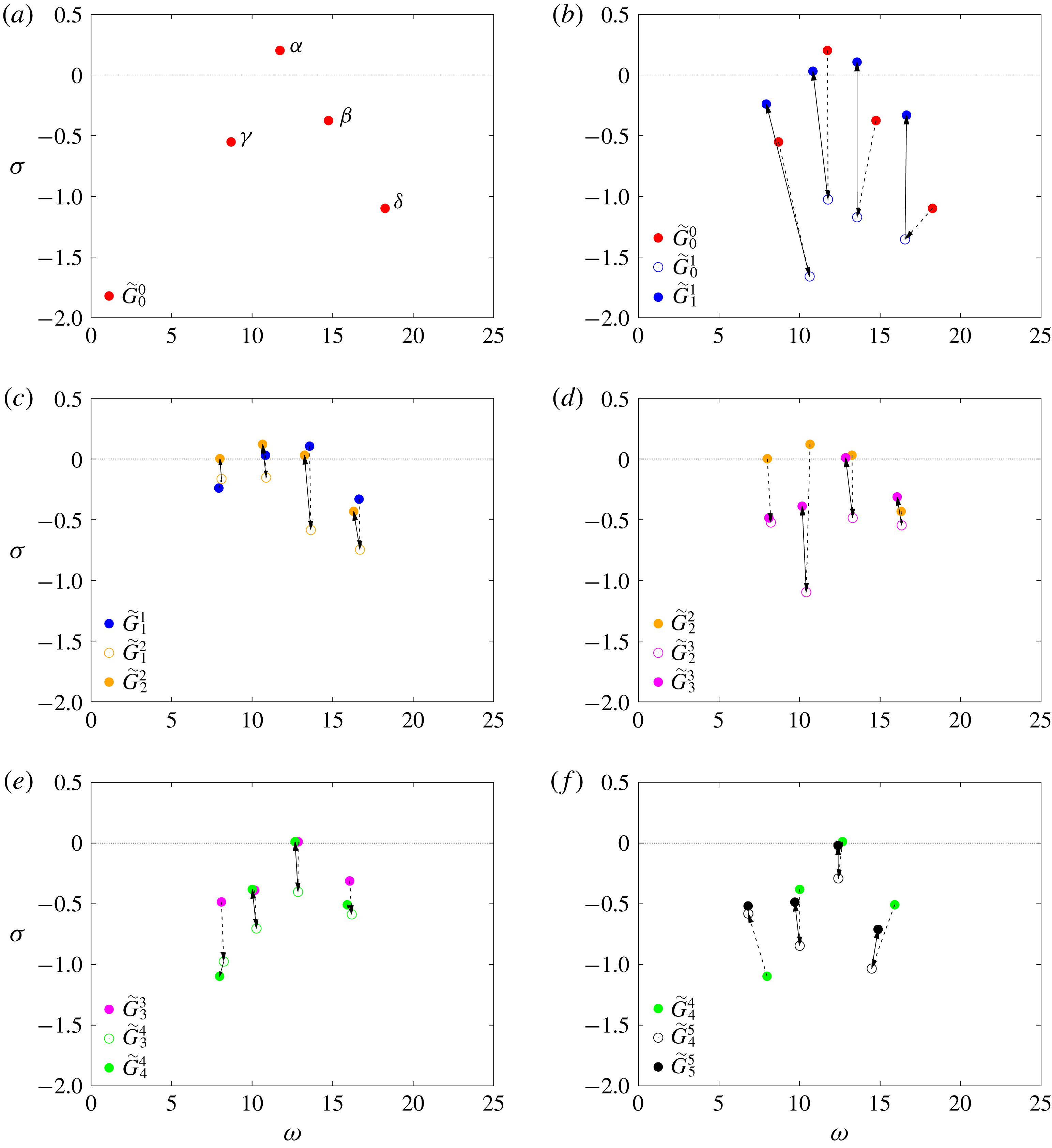
Second, instead of designing a new controller
 $K_{m+1}$
from the sole knowledge of the mean flow
 $m$
, we design a controller correction
 $K_{m+1}^{\prime }=K_{m+1}-K_{m}$
based on the knowledge of both the mean flow
 $m$
and the controller
 $K_{m}$
. Again, we are not following the transient evolution of a globally stable flow, but a sequence of permanent states visited by an unstable flow coupled with some controllers. The plant model
 $G_{m}^{0}$
based on the mean flow
 $m$
alone does not characterize the response to a small change in actuation of the coupled system, and the adequate transfer function is
 $G_{m}^{m}$
. As can be seen in figure 18 for
 $m=5$
, the transfer functions
 $G_{m}^{0}$
and
 $G_{m}^{m}$
may be quite different indeed.
Comparison between the gain of the transfer functions
 $G_{5}^{0}=G_{b}$
associated with the base flow only and
 $G_{5}^{5}$
, the transfer function associated with the closed loop between the base flow and the final controller
 $K_{5}$
.

Finally, in Högberg et al. (Reference Högberg, Bewley and Henningson2003), the order of the controller remains fixed during the iteration whereas that of the total controller
 $K_{m}=\sum _{j=1}^{m}K_{j}^{\prime }$
increases in our case. This drawback of our approach may not be an issue for implementation, since each control law
 $u_{j}^{\prime }$
may be computed independently, and then added to form
 $u_{m}=\sum _{j=1}^{m}u_{j}^{\prime }$
. Since each
 $K_{j}^{\prime }$
has the same order, the computational cost increases only linearly with the number of iterations
 $m$
. The computational time may even be kept constant using parallel computing. Alternatively, a low-order model may be obtained from the total controller
 $K_{m}$
at each step. In our case, we successfully reduced the number of states of
 $K_{5}$
from 50 to 12 with no loss in performance (using the modred command from MATLAB, which is based on balanced truncation).
7 Conclusion
The present study proposes a novel approach for the control of strongly nonlinear resonating flows using linear methods only. The approach is illustrated on the case of open-cavity flow at
 $Re=7500$
, i.e. far from the linear instability threshold which is at
 $Re_{c}=4140$
. Starting from a quasiperiodic unactuated regime, we manage to completely suppress the oscillations with a sequence of five robust controllers. At the end of the process, the base flow is reached, with stabilized linear dynamics. The method relies on two key ideas:
(i) modelling of the system as an LTI plant using the resolvent operator about the mean flow,
(ii) a Newton-type iterative procedure based on the successive mean flows.
The first point (i) builds on previous observations that linear analysis about the mean state yields quantitative information about the underlying nonlinear dynamical equilibrium. Modal analysis is indeed able to capture the structure and frequencies of self-sustained oscillations, while resolvent analysis successfully captures receptivity to forcing, even in turbulent flows. Using the resolvent operator in order to derive a sequence of input–output models, we show that it takes no more than a series of time-averaged flows to design a successful feedback loop. Not only is the method simple, general and computationally inexpensive, it is also physically insightful. Furthermore, LTI models of nonlinear flows derived from the mean state are also unambiguously defined, as opposed to linear models identified from input–output data. This is particularly useful in the case of unstable base flows, which inevitably lead to nonlinear dynamics even in the most quiet environment. When the base flow is reached, the system is truly linear and the proposed definition matches exactly with the actual definition of the transfer function. In essence, the framework initially introduced by McKeon & Sharma (Reference McKeon and Sharma2010) naturally lends itself to the modelling of an LTI input–output relation for nonlinear flows. Although seemingly optimal in some sense, there is however no proof that the resolvent operator about the mean flow is the best option, or work in every cases, and these questions will be addressed in future work.
The second point (ii) also appears to be fairly novel, although it is in principle independent of (i), which means that an iterative procedure could also be carried out with a different modelling strategy for defining an LTI model at each step. The key idea here is to resort to a sequence of linear approximations in order to solve a nonlinear control problem. For sufficiently strong nonlinearity, designing a single low-dimensional LTI controller able to destroy the initial attractor and drive the system directly to the fixed point is a challenge. Instead of designing complex nonlinear models, or crafting elaborate nonlinear control laws, we propose to use a simple sequence of linear controllers. Each controller disrupts the current dynamical equilibrium and drives the system to a new one, closer to the fixed point in phase space. After a few iterations, the coupled system becomes attracted to the fixed point and flow oscillations are fully suppressed. Note that although only linear controllers are used, the entire procedure is nonlinear in essence, as the effect of each controller depends fundamentally on the choice of the past controllers. And although the final controller stabilizes the base flow once reached, it is not guaranteed to drive the system from an initial condition on the attractor to the base flow. The method set forth in this paper is in some sense analogue to Newton’s iteration: a series of linear models and controllers are derived, until fluctuations arising from nonlinearity are fully cancelled.
From a practical perspective, the proposed method has one clear advantage: it only requires knowledge of the mean flow, at every iteration. There is no need for an adjoint simulation either, and, in the case of turbulent flows, the method might be applicable from a time-averaged unsteady RANS simulation. Computing the transfer function requires the formation of the Jacobian matrix, followed by the resolution of a linear system for each frequency. For two-dimensional, or equivalently three-dimensional problems with one invariant direction, this is computationally inexpensive. For fully three-dimensional mean flows, matrix-free methods may be considered instead. A disadvantage of the method though, is that it requires knowledge of the full mean state. However, data assimilation is an active field of research in fluid mechanics, and techniques have recently been developed for two-dimensional mean-flow reconstruction from under-resolved/incomplete/noisy measurements (Foures et al. Reference Foures, Dovetta, Sipp and Schmid2014; Symon et al. Reference Symon, Dovetta, McKeon, Sipp and Schmid2017). For the method to be applicable outside the laboratory however, methods should be developed to infer the mean flow from localized sensors only.
Future work will be dedicated to understanding the rationale behind the success of mean-flow-based input–output models and their limitations. It would also be interesting to analyse the convergence properties of the iterative method from a theoretical viewpoint. Applicability of the method to noise amplifiers, chaotic flows and turbulent flows also remains to be investigated.
Acknowledgements
Enlightening discussions with É. Garnier, N. Fabbiane, Navrose, O. Marquet and Y. Duguet are gratefully acknowledged. The authors are also grateful to M. Juniper for sharing his MATLAB toolbox for the analysis of nonlinear dynamics (Juniper & Sujith Reference Juniper and Sujith2018).