



Nomenclature
-
 $a,b$
-
plate planar dimensions
- ANM
-
Asymptotic-Numerical Method
-
$\boldsymbol{c}$
-
vector of unknown amplitudes
-
$e$
-
stiffener eccentricity
-
${\textit{E}}{\rm{\;\;\;\;\;\;\;\;\;\;\;\;\;\;\;\;\;\;\;\;\;\;}}$
-
elastic modulus
-
$\boldsymbol{F}\;$
-
external load
- FSDT
-
First-order Shear Deformation Theory
-
${\textit{G}}$
-
shear modulus
-
$h$
-
plate thickness
-
${h_s}\;$
-
stiffener height
-
$\boldsymbol{\mathcal{J}}$
-
rotation conventions
-
${J_s}$
-
Jacobian of the transformation
-
$k$
-
Lagrange multiplier
-
$\boldsymbol{K}$
-
stiffness matrix
-
$\boldsymbol{L},\boldsymbol{Q},\boldsymbol{C},$
-
linear, quadratic and cubic operators
-
$N$
-
order of the expansion
-
${N_s}$
-
number of stringers
- NR
-
Newton-Raphson
-
${{\boldsymbol{P}}_i}$
-
stiffener control points coordinates
-
${\boldsymbol{R}}$
-
rotation matrix
-
${{\textit{R}}},{{\textit{S}}}{\rm{\;\;\;\;\;\;\;\;\;\;}}$
-
number of trial functions
-
$s,n,b$
-
stiffener reference system
-
${t_s}$
-
stiffener thickness
-
$u,v,w$
-
plate generalised displacements
-
${u_t},{v_n},{w_b}$
-
stiffener generalised displacements
- VS
-
Variable Stiffness
-
$x,y,z$
-
plate reference system


Greek symbol
-
$\alpha $
-
arc-length parameter
-
$\boldsymbol\epsilon,\boldsymbol\gamma $
-
plate generalised strain
-
${\boldsymbol\epsilon _s}$
-
stiffener generalised strain
-
$\delta {\boldsymbol\epsilon _s}$
-
virtual variation of the stiffener generalised strain
-
$\epsilon$
-
heuristic parameter to estimate the radius of convergence
-
$\theta $
-
fiber orientation angle
-
${\theta _t},{\theta _n},{\theta _b}$
-
stiffener generalised rotations
-
$\lambda $
-
load parameter
-
${\lambda _{cr}}$
-
buckling parameter
-
$\boldsymbol\nu $
-
Poisson ratio
-
$\xi, \eta $
-
plate dimensionless coordinates
-
${\varphi _x},{\varphi _y},{\varphi _z}$
-
plate generalised rotations


1.0 Introduction
Over the past years, the development of new manufacturing techniques – automated fiber placement, automated tape laying and addictive manufacturing are among the most important – allowed new and innovative load-carrying aeronautical structures to be explored. Two meaningful examples are variable stiffness (VS) and curvilinearly stiffened panels. Variable Stiffness (VS) configurations are a promising solution. These structures are developed with a variable stiffened skin, in which the fibers are allowed to vary their orientation as a function of the planar position. In addition, extra tailoring capabilities can be reached by introducing stiffeners with curvilinear, rather than conventional straight, paths. The design of panels with non-uniform elastic properties, such as in the cases outlined above, allows structural efficiency to be improved, with a drastic potential on structural weight saving. Previous works in the literature compared the efficiency of VS laminates configurations in terms of mechanical buckling [Reference Tatting and Gürdal1–Reference Wu, Raju and Weaver7, Reference Olmedo and Gürdal53], thermal buckling [Reference Vescovini and Dozio8, Reference Oliveri, Milazzo and Weaver9], fundamental frequencies [Reference Akhavan and Ribeiro10, Reference Yazdani and Ribeiro11] and failure loads [Reference Lopes, Camanho, Gürdal and Tatting12]. Ritz-based approaches are particularly suitable for the analysis of VS configurations due to the relatively low number of degrees of freedom to obtain accurate results. A Ritz-like approach is employed in Refs. [Reference Wu, Raju and Weaver5, Reference Wu, Raju and Weaver6], where a mixed formulation and thin-plate theory are applied to buckling and post-buckling problems; instead, a Galerkin formulation is introduced in the work [Reference Senocak and Tanriover13] to solve plane stress problem of VS plates. The current interest for using VS configurations in real-life applications is corroborated by ongoing experimental campaigns, such as the one presented in Ref. [Reference Zucco, Oliveri, Rouhi, Telford, Clancy, McHale, O’Higgins, Young, Weaver and Peeters14]. In the referenced work, a VS unitised integrated-stiffener out-of-autoclave thermoplastic composite wingbox is tested for studying the buckling response due to combined shear-bending-torsion.
The literature on curvilinearly stiffened panels is more scarce with respect to the one on VS composites. Indeed challenges exist both from technological and modeling perspectives. Recent advances on additive manufacturing opened the door to easier fabrication of these structures, in most cases with isotropic materials. Regarding the modeling aspects, difficulties arise due to the inherent complexity of the geometrical pattern. This aspect, in turn, requires careful handling of the computational grid and effective strategies for the enforcement of the compatibility between the skin and the stringer. Within a finite element framework, the definition of these compatibility requirements can be relatively cumbersome. Indeed, node sharing between skin and stiffener requires careful meshing to prevent element distortion. Locatelli et al. [Reference Locatelli, Mulani and Kapania15] developed a tool that automatically generates the geometry and performs the re-meshing for every variation in the structure configuration. An alternative approach relies on contact algorithms or ad-hoc finite element formulations, as the ones outlined by Refs. [Reference Shi, Kapania and Dong16–Reference Zhao and Kapania18]. In these works, finite element shape functions are employed to express stiffeners displacements as a function of the skin ones. So, the skin and the stiffener elements are independent from one another and node sharing between them is not needed. Another strategy involves the use of mesh-free methods, as the element-free Galerkin and the Ritz method, see Refs. [Reference Tamijani and Kapania19–Reference Tamijani and Kapania21, Reference Tamijani, McQuigg and Kapania52], in which free-vibration, bending and buckling problems are considered.
The individual advantages offered by VS skins and curvilinear stringers suggest the opportunity to consider both these features combined together. Recently, Singh and Kapania [Reference Singh and Kapania22] showed how the buckling load can be increased if curvilinear stiffeners are employed. An optimisation framework is discussed in Ref. [Reference Singh and Kapania23] to design tow-steered composite laminates with metallic curvilinear stiffeners. Goal of the optimisation is maximising the buckling load, while minimising the mass of the panels. In the works by Zhao and Kapania [Reference Zhao, Singh and Kapania24–Reference Zhao and Kapania26] ad-hoc finite element models are developed for the analysis of curvilinearly stiffened panels in terms of free-vibration, thermal buckling and thermo-mechanical buckling behaviour, respectively.
Even though numerical studies on curvilinearly stiffened VS panels are available, experimental campaigns, to the best of the authors’ knowledge, are still lacking. Nevertheless, the study of these structures is of interest for future applications. Aside from the current technological capabilities, the investigation of any potential advantage could stimulate new manufacturing techniques to be developed. A first step to conduct the mentioned assessments involves the development of appropriate analysis tools.
The investigation on curvilinearly stiffened VS skins is extended to a Ritz-based approach in recent works of the authors [Reference Vescovini, Oliveri, Pizzi, Dozio and Weaver27, Reference Vescovini, Oliveri, Pizzi, Dozio and Weaver28], and excellent computational efficiency was demonstrated for free-vibration, buckling and thermal buckling problems. In a recent work [Reference Vescovini and Foligno29], the Ritz framework is extended to account for post-buckling analysis capabilities. For this purpose, an iterative-incremental procedure is developed based on the Newton-Raphson method. To keep the computational burden at minimum, special care is given to the implementation of the non-linear terms, which are expressed in a suitable way to minimise the number of operations to be conducted. The so-obtained computational tool guarantees satisfactory computational time, although the advantage over finite elements is not as drastic as it is for linear analyses. Indeed, spectral approaches, such as the Ritz method, are inherently associated with computationally expensive operations when non-linear terms are of concern. One possibility to speed-up the time for the solution involves the adoption of an effective solution method, capable of providing improved performance with respect to Newton-Raphson. For this purpose, the Asymptotic-Numerical Method (ANM) is proposed here as an excellent mean to improve the Ritz-based tool for the non-linear post-buckling analysis presented in the previous effort [Reference Vescovini and Foligno29]. The ANM was proposed several years ago by Potier-Ferry and co-workers. In Ref. [Reference Damil and Potier-Ferry30], the ANM was developed to compute perturbed bifurcations. In subsequent works [Reference Cochelin31–Reference Azrar, Cochelin, Damil and Potier-Ferry34], the method was applied for the post-buckling solution of elastic plates and in a finite element environment. An extensive review on the ANM algorithm can be found in the work of Potier-Ferry and Cadou [Reference Potier-Ferry and Cadou35].
1.1 Aims and objectives
Due to the large number of design variables offered by innovative VS configurations, the development of fast analysis tools is of paramount importance, especially when the non-linear response is of concern. With this consideration in mind, this work aims at presenting an advanced Ritz-based formulation that exploits the ANM for the analysis of curvilinearly stiffened panels. The result is an effective computational tool to analyse the post-buckling response of relatively complex configurations with reduced modeling and computational effort. The proposed tool will serve in the future as a mean to investigate any potential gain offered by curvilinearly stiffened panels including post-buckling design considerations.
The paper is organised as follows: Section 2 offers a general framework of the non-linear problem formulation; starting from the structural configuration, the skin and the stiffener models are presented, along with the perturbation technique and the numerical approximation; Section 3 illustrates the comparison against Abaqus finite element results and a Ritz-based approach based on the Newton-Raphson method; limitations of the current work, conclusions and future developments are summarised in Sections 4 and 5.
2.0 Formulation
The semi-analytical formulation for the post-buckling analysis of curvilinearly stiffened panels is presented in this section. Firstly, the structure under investigation is described: the plate and stiffener models are illustrated with special care on the parameterisation technique for the stiffeners path. Then, the perturbation technique and the numerical solution procedure are presented in detail.
2.1 Structural configuration
The structure is the assembly of two different components: a VS skin and an arbitrary number
 ${N_s}$
of curvilinear stringers. A sketch of the structure is available in Fig. 1(a). A two-dimensional plate model is considered for the skin and a one-dimensional beam model for the stiffeners. The reference systems and the relevant dimensions are available in Fig. 1. A Cartesian reference system
 $xyz$
is considered with the origin located in the middle of the plate midsurface, in which
 $x$
and
 $y$
are the longitudinal and transverse axes, respectively, whereas
 $z$
is taken in the thickness direction. The plate has dimensions equal to
 $a$
and
 $b$
and thickness
 $h$
. The second structural components are the stiffeners. They are assumed to be blade-shaped and obtained by the stacking of plies with constant orientation. The height and width are equal to
 ${h_s}$
and
 ${t_s}$
, respectively. A local reference system
 $snb$
is taken at the origin of the reference system on the plate midsurface. This choice simplifies the enforcement of the compatibility conditions between plate and stiffener. The skin is obtained by the stacking of plies with curvilinear fibers. For the stringers, straight-fiber plies with orthotropic sequence are stacked along the width direction. Hence, fiber orientation is constant along the stiffener axis. The panel can be constrained at the outer edges with any boundary condition, including free, simply supported and clamped ones.
Sketch of the curvilinearly stiffened panel: (a) dimensions; (b) fiber paths; (c) conventions for the generalised displacements and rotations.

The kinematic assumptions adopted for the skin are suitable for thin up to moderately thick panels, which are commonly used in aeronautical applications. Concerning the stiffeners, the beam-like model is neither able to account for local instabilities and section deformability effects, nor to provide refined modeling of the coupling with the skin. Nonetheless, such behaviours are usually crucial in the deep post-buckling field, therefore the present model is believed adequate for assessments on the initial post-buckling [Reference Bisagni and Vescovini36–Reference Huang and Qiao40].
The section properties can be determined for different shapes, including blade, T or J stringers. Irrespective of the shape, the beam model is fully determined by the axial, bending, shear and torsional stiffnesses. Without loss of generality, blade stringers are considered in this work. Other shapes can be easily modeled by evaluating the section properties following analytical approaches, such as the one outlined in Ref. [Reference Barbero, Lopez-Anido and Davalos41]. More advanced semi-analytical strategies can be considered too [Reference Giavotto, Borri, Mantegazza, Ghiringhelli, Carmaschi, Maffioli and Mussi42].
2.1.1 Skin model
Lagrange polynomials interpolation is employed to take into account the VS properties of the skin. A grid of
 $M \times N$
points is considered, where the orientation angles
 ${\theta _{mn}}$
are specified over one quarter of the plate, as depicted in Fig. 1(b). The orientation angle in a generic point is evaluated as [Reference Wu, Weaver, Raju and Kim43]:
 \begin{align}\theta \left( {x,y} \right) = \mathop \sum \limits_{m = 0}^{M - 1} \mathop \sum \limits_{n = 0}^{N - 1} {\theta _{mn}}\mathop \prod \limits_{m \ne i} \left( {{{\left| x \right| - {x_i}} \over {{x_m} - {x_i}}}} \right)\mathop \prod \limits_{n \ne j} \left( {{{\left| y \right| - {y_j}} \over {{y_n} - {y_j}}}} \right)\end{align}
where the angle
 $\theta $
is allowed to vary with non-linear law in the coordinates
 $x$
and
 $y$
. A linear fiber variation is achieved by considering two points only, one at the centre and the other at the edge of the plate.
The plate kinematics is modelled according to the First-order Shear Deformation Theory (FSDT). Despite more refined results can be obtained if higher-order theories are employed [Reference Pagani and Sánchez-Majano44–Reference Vescovini and Dozio46], this approach is believed adequate for preliminary calculations for thin aeronautical panels. Based on FSDT, the displacement of a generic point of the surface can be written as [Reference Reddy47]:
 \begin{equation}\begin{split}\textbf{u}(x,y,z) =\begin{Bmatrix} u(x,y,z)\\[5pt] v(x,y,z)\\[5pt] w(x,y,z)\end{Bmatrix}&=\begin{Bmatrix} u^0(x,y)\\[5pt] v^0(x,y)\\[5pt] w^0(x,y)\end{Bmatrix}+ z\begin{bmatrix} 1 & 0 & 0\\[5pt] 0 & 1 & 0\\[5pt] 0 & 0 & 0\\[5pt] \end{bmatrix}\begin{Bmatrix} \varphi_x(x,y)\\[5pt] \varphi_y(x,y)\\[5pt] \varphi_z(x,y)\end{Bmatrix}\\[5pt] &= \textbf{u}^0(x,y) + z \textbf{L} \, \boldsymbol{\varphi}(x,y)\\[5pt] &=\begin{bmatrix}\textbf{I} & z\,\textbf{L}\end{bmatrix}\begin{Bmatrix}\textbf{u}^0(x,y)\\[5pt] \boldsymbol{\varphi}(x,y)\end{Bmatrix}=\begin{bmatrix}\textbf{I} & z\,\textbf{L}\end{bmatrix}\textbf{d}_0\end{split}\end{equation}
where
 ${{\textbf{u}}^0}$
and
 $\varphi $
are the linear displacements and rotations of the midsurface and
 ${{\textbf{d}}_0}$
is the vector collecting them. The conventions for the generalised displacements and rotations are shown in Fig. 1(c). The non-linear strain components are computed from the expression of the Green-Lagrange strain tensor under the von Kármán approximation:
 \begin{align}&\boldsymbol{\epsilon} =\begin{Bmatrix} \epsilon^0_{xx}\\[5pt] \epsilon^0_{yy}\\[5pt] \gamma^0_{xy}\end{Bmatrix}+ z\begin{Bmatrix} k_{xx}\\[5pt] k_{yy}\\[5pt] k_{xy}\end{Bmatrix}= \boldsymbol{\epsilon}^0 + z \, \textbf{k}\end{align}
 \begin{align}&\boldsymbol{\gamma} =\begin{Bmatrix} \gamma_{yz}\\[5pt] \gamma_{xz}\end{Bmatrix}\end{align}
where:
 \begin{align}&\boldsymbol{\epsilon}^0 =\begin{Bmatrix} u^0_{/x} + \frac{1}{2} \left( w^0_{/x} \right)^2 + w^0_{/x} \, w^*_{/x}\\[5pt] v^0_{/y} + \frac{1}{2} \left( w^0_{/y} \right)^2 + w^0_{/y} \, w^*_{/y}\\[5pt] u^0_{/y} + v^0_{/x} + w^0_{/x} w^0_{/y} + w^0_{/x} w^*_{/y} + w^0_{/y} \, w^*_{/x}\end{Bmatrix}\end{align}
 \begin{align}&\textbf{k} =\begin{Bmatrix} \varphi_{x/x}\\[5pt] \varphi_{y/y}\\[5pt] \varphi_{x/y} + \varphi_{y/x}\end{Bmatrix}, \; \; \; \boldsymbol{\gamma} =\begin{Bmatrix} \varphi_x + w^0_{/x}\\[5pt] \varphi_y + w^0_{/y}\end{Bmatrix} \end{align}
Previous studies in the literature [Reference Garcea, Madeo and Casciaro48, Reference Garcea, Madeo and Casciaro49] have shown the inadequacy of the von Kármán non-linear approach when large displacements and rotations are of concern, such as in the case of cantilever beams. However, typical conditions for wing and fuselage panels involve the panel’s edges to be assumed as simply supported or clamped. In these cases, von Kármán theory proved to be adequate. In Equations (3) and (5),
 ${w^{\rm{*}}}$
is the initial imperfections and
 ${(\!\cdot\!)_{/x}}$
and
 ${(\!\cdot\!)_{/y}}$
express the derivatives with respect to the in-plane coordinates.
The strain virtual variations are written as a function of the displacement field as:
 \begin{align}\delta {\boldsymbol\epsilon ^0} = {{\textbf{G}}_1}\left( {{{\textbf{d}}_0}} \right){{\textbf{G}}_2}\delta {{\textbf{d}}_0}\end{align}
 \begin{align}\delta {\textbf{k}} = {{\textbf{G}}_k}{\rm{\;}}\delta {{\textbf{d}}_0}\end{align}
 \begin{align}\delta \boldsymbol\gamma = {{\textbf{G}}_\gamma }{\rm{\;}}\delta {{\textbf{d}}_0}\end{align}
where the matrices
 ${{\textbf{G}}_1}\left( {{{\textbf{d}}_0}} \right)$
,
 ${{\textbf{G}}_2}$
,
 ${{\textbf{G}}_k}$
and
 ${{\textbf{G}}_\gamma }$
are defined as:
 \begin{align}&\textbf{G}_1 (\textbf{d}_0) \textbf{G}_2 =\begin{bmatrix}1\;\;\;\;\; & 0\;\;\;\;\; & 0\;\;\;\;\; & 0\;\;\;\;\; & w_{/x}^0 + w_{/x}^*\;\;\;\;\; & 0\\[5pt] 0\;\;\;\;\; & 0\;\;\;\;\; & 0\;\;\;\;\; & 1\;\;\;\;\; & 0\;\;\;\;\; & w_{/y}^0 + w_{/y}^*\\[5pt] 0\;\;\;\;\; & 1\;\;\;\;\; & 1\;\;\;\;\; & 0\;\;\;\;\; & w_{/y}^0 + w_{/y}^*\;\;\;\;\; & w_{/x}^0 + w_{/x}^*\end{bmatrix}\begin{bmatrix}(\!\cdot\!)_{/x}\;\;\;\;\; & 0\;\;\;\;\; & 0\;\;\;\;\; & 0\;\;\;\;\; & 0\;\;\;\;\; & 0\\[5pt] (\!\cdot\!)_{/y}\;\;\;\;\; & 0\;\;\;\;\; & 0\;\;\;\;\; & 0\;\;\;\;\; & 0\;\;\;\;\; & 0\\[5pt] 0\;\;\;\;\; & (\!\cdot\!)_{/x}\;\;\;\;\; & 0\;\;\;\;\; & 0\;\;\;\;\; & 0\;\;\;\;\; & 0\\[5pt] 0\;\;\;\;\; & (\!\cdot\!)_{/y}\;\;\;\;\; & 0\;\;\;\;\; & 0\;\;\;\;\; & 0\;\;\;\;\; & 0\\[5pt] 0\;\;\;\;\; & 0\;\;\;\;\; & (\!\cdot\!)_{/x}\;\;\;\;\; & 0\;\;\;\;\; & 0\;\;\;\;\; & 0\\[5pt] 0\;\;\;\;\; & 0\;\;\;\;\; & (\!\cdot\!)_{/y}\;\;\;\;\; & 0\;\;\;\;\; & 0\;\;\;\;\; & 0\end{bmatrix} \end{align}
 \begin{align}&\textbf{G}_{k} =\begin{bmatrix}0\;\;\;\;\; & 0\;\;\;\;\; & 0\;\;\;\;\; & (\!\cdot\!)_{/x}\;\;\;\;\; & 0\;\;\;\;\; & 0\\[5pt] 0\;\;\;\;\; & 0\;\;\;\;\; & 0\;\;\;\;\; & 0\;\;\;\;\; & (\!\cdot\!)_{/y}\;\;\;\;\; & 0\\[5pt] 0\;\;\;\;\; & 0\;\;\;\;\; & 0\;\;\;\;\; & (\!\cdot\!)_{/y}\;\;\;\;\; & (\!\cdot\!)_{/x}\;\;\;\;\; & 0\\[5pt] \end{bmatrix} \end{align}
 \begin{align}& \textbf{G}_{\gamma} =\begin{bmatrix}0\;\;\;\;\; & 0\;\;\;\;\; & (\!\cdot\!)_{/x}\;\;\;\;\; & 1\;\;\;\;\; & 0\;\;\;\;\; & 0\\[5pt] 0\;\;\;\;\; & 0\;\;\;\;\; & (\!\cdot\!)_{/y}\;\;\;\;\; & 0\;\;\;\;\; & 1\;\;\;\;\; & 0\\[5pt] \end{bmatrix}\end{align}
2.1.2 Stiffener model
The stiffener path is parameterised using Bézier curves [Reference Dang, Kapania, Slemp, Bhatia and Gurav50]. This choice originates from the popularity of this curve representation. Their definition is straightforward and is briefly outlined below. One potential disadvantage is given by the position of the control points, which generally do not belong to the curve. Strategies other than Bézier curves are equally possible, such as NURBS or Hobby splines (see Refs. [Reference Zhao and Kapania17, Reference Zhao, Singh and Kapania25]). They are not investigated here, but the method could be easily modified to incorporate them. Therefore, the stiffener coordinates are expressed through the relation
 ${\textbf{x}} = {\textbf{r}}\left( p \right)$
, with:
 \begin{align}\textbf{r}(p) = \sum_{i=0}^n \binom{n}{i} \, \textbf{P}_i \, \left(1-\frac{p+1}{2}\right)^{n-i} \, \left(\frac{p+1}{2}\right)^i\end{align}
where
 $n$
is the order of the polynomial,
 ${{\textbf{P}}_i}$
are the coordinates of the control points and
 $p \in \left[ { - 1{\rm{\;\;\;\;}}1} \right]$
. In the present work,
 ${2^{nd}}$
and
 ${3^{rd}}$
order curves are employed, whose expression reads:
 \begin{align}&\textbf{r}(p) = \frac{1}{4} (1-p)^2 \textbf{P}_0 + \frac{1}{2}(1-p^2)\textbf{P}_1 + \frac{1}{4}(1+p)^2\textbf{P}_2\end{align}
 \begin{align}{\textbf{r}}\left( p \right) = \frac{1}{8}{(1 - p)^3}{{\textbf{P}}_0} + \frac{3}{8}\left( {1 + p} \right){(1 - p)^2}{{\textbf{P}}_1} + \frac{3}{8}{(1 + p)^2}\left( {1 - p} \right){{\textbf{P}}_2} + \frac{1}{8}{(1 + p)^3}{{\textbf{P}}_3}\end{align}
Given the stiffener path, the unit tangent vector can be evaluated as:
 \begin{align}{\textbf{t}}\left( s \right) = {{\textbf{x}}_{/s}}\left( s \right) = \frac{{{{\textbf{x}}_{/p}}\left( s \right)}}{{\left| {{{\textbf{x}}_{/p}}\left( s \right)} \right|}}\end{align}
where
 $s$
is the arc-length coordinate. From Equation (16), the relation between their differentials can be derived:
 \begin{align}ds = \left| {{{\textbf{x}}_p}} \right|{\rm{\;}}dp = {J_s}{\rm{\;}}dp\end{align}
 \begin{align}{(\!\cdot\!)_{/s}} = \frac{1}{{{J_s}}}{\rm{\;}}{(\!\cdot\!)_{/p}}\end{align}
where
 ${J_s}$
is the Jacobian of the transformation. The normal vector
 ${\textbf{n}}$
is obtained by rotating the tangent vector of Equation (16) in counterclockwise direction by
 $\pi /2$
; the binormal vector
 ${\textbf{b}}$
is directed as the plate normal positive direction. The variation of the unit vectors along the curve is evaluated via Frenet formulas [Reference Martini and Vitaliani51]:
 \begin{align}\begin{array}{*{20}{l}}{} {}{{{\textbf{t}}_{/s}}\left( s \right) = \kappa \left( s \right){\rm{\;}}{\textbf{n}}\left( s \right)}\\[5pt] {} {}{{{\textbf{n}}_{/s}}\left( s \right) = - \kappa \left( s \right){\rm{\;}}{\textbf{t}}\left( s \right) + \tau \left( s \right){\rm{\;}}{\textbf{b}}\left( s \right)}\\[5pt] {} {}{{{\textbf{b}}_{/s}}\left( s \right) = - \tau \left( s \right){\rm{\;}}{\textbf{n}}\left( s \right)}\end{array}\end{align}
The stiffeners are modelled as Timoshenko beam elements, hence the generalised displacement components are expressed as:
 \begin{align}{{\textbf{u}}_s}\left( {s,n,b} \right) = {\textbf{u}}_s^0\left( s \right) + {(\textbf{d} \times )^T}{\theta _s}\left( s \right)\end{align}
with:
 \begin{align}{\textbf{u}}_s^0\left( s \right) = u_t^0\left( s \right){\rm{\;}}{\textbf{t}} + v_n^0\left( s \right){\rm{\;}}{\textbf{n}} + w_b^0\left( s \right){\rm{\;}}{\textbf{b}}\end{align}
 \begin{align}\boldsymbol{\theta}_s(s) = \theta_t(s)\, \textbf{t} + \theta_n(s)\, \textbf{n} + \theta_b(s)\, \textbf{b}\end{align}
 \begin{align}{\textbf{d}} = n{\rm{\;}}{\textbf{n}} + b{\rm{\;}}{\textbf{b}}\end{align}
where
 $snb$
is a local reference frame with origin on the plate midsurface. Note, displacements and rotations are expressed as a function of the plate kinematics, so no independent degrees of freedom are associated with the stringers, with clear advantages of the final size of the problem. The second order tensor
 ${\textbf{d}} \times $
in Equation (20) is defined such that
 $\left( {{\textbf{d}} \times } \right){\rm{\;}}{\textbf{a}} = {\textbf{d}} \times {\textbf{a}}$
, for any vector
 ${\textbf{a}}$
. The conventions for the stiffener kinematics are depicted in Fig. 1(c).
The strains are readily derived from the kinematic assumptions of Equation (20) as:
 \begin{align}\boldsymbol{\epsilon}_s =\begin{Bmatrix} \epsilon_t\\[5pt] \gamma_n\\[5pt] \gamma_t\end{Bmatrix}= \boldsymbol{\epsilon}_s^0 + (\textbf{d} \times)^T \, \textbf{k}_s =\begin{Bmatrix} \epsilon_t^0 + b\, k_n - n\, k_b\\[5pt] \gamma_n^0 - b\, k_t\\[5pt] \gamma_b^0 + n\, k_t\end{Bmatrix}\end{align}
with:
 \begin{align}&\boldsymbol{\epsilon}_s^0 =\begin{Bmatrix} \epsilon_t^0\\[5pt] \gamma_n^0\\[5pt] \gamma_b^0\end{Bmatrix}=\begin{Bmatrix} \frac{\partial u_t^0}{\partial s} - \kappa (s)\, v_n^0 +\frac{1}{2} \left ( \frac{\partial w_b^0}{\partial s} \right )^2\\[5pt] \frac{\partial v_n^0}{\partial s} + \kappa (s)\, u_t^0 - \theta_b\\[5pt] \frac{\partial w_b^0}{\partial s} + \theta_n\end{Bmatrix}&\textbf{k}_s =\begin{Bmatrix} k_t\\[5pt] k_n\\[5pt] k_b\end{Bmatrix}=\begin{Bmatrix} \frac{\partial \theta_t}{\partial s} - \kappa (s)\, \theta_n\\[5pt] \frac{\partial \theta_n}{\partial s} + \kappa (s)\, \theta_t\\[5pt] \frac{\partial \theta_b}{\partial s}\end{Bmatrix}\end{align}
Note that von Kármán assumptions are introduced in Equation (25), so the only non-linear contribution involves the quadratic term in the unknown
 ${w_b}$
.
After introducing the vector
 ${\textbf{d}}_0^s = {\{ {\textbf{u}}_s^0{\rm{\;\;\;\;\;\;}}{\theta _{\textbf{s}}}\} ^T}$
, the strain virtual variations can be expressed as:
 \begin{align}\delta {\boldsymbol\epsilon _s} = {\mathcal{D}_1}\left( {{\textbf{d}}_0^s} \right){\rm{\;\;}}\delta {\textbf{d}}_0^s\end{align}
where the matrix
 ${\mathcal{D}_1}\left( {{\textbf{d}}_0^s} \right)$
is defined as:
 \begin{equation}\boldsymbol{\mathcal{D}}_1(\textbf{d}_0^s) =\begin{Bmatrix} (\!\cdot\!)_{/s}\;\;\;\;\; & - \kappa(s)\;\;\;\;\; & w^0_{b/s} \, (\!\cdot\!)_{/s}\;\;\;\;\; & 0\;\;\;\;\; & 0\;\;\;\;\; & 0\\[5pt] \kappa(s)\;\;\;\;\; & (\!\cdot\!)_{/s}\;\;\;\;\; & 0\;\;\;\;\; & 0\;\;\;\;\; & 0\;\;\;\;\; & -1\\[5pt] 0\;\;\;\;\; & 0\;\;\;\;\; & (\!\cdot\!)_{/s}\;\;\;\;\; & 0\;\;\;\;\; & 1\;\;\;\;\; & 0\\[5pt] 0\;\;\;\;\; & 0\;\;\;\;\; & 0\;\;\;\;\; & (\!\cdot\!)_{/s}\;\;\;\;\; & -\kappa(s)\;\;\;\;\; & 0\\[5pt] 0\;\;\;\;\; & 0\;\;\;\;\; & 0\;\;\;\;\; & \kappa(s)\;\;\;\;\; & (\!\cdot\!)_{/s}\;\;\;\;\; & 0\\[5pt] 0\;\;\;\;\; & 0\;\;\;\;\; & 0\;\;\;\;\; & 0\;\;\;\;\; & 0\;\;\;\;\; & (\!\cdot\!)_{/s}\end{Bmatrix}\end{equation}
The compatibility between the stringers and the skin is enforced in a strong-form manner. The procedure follows the approach outlined in Ref. [Reference Vescovini, Oliveri, Pizzi, Dozio and Weaver28] and consists in expressing the beam kinematics as a function of the plate generalised displacements as:
 \begin{align}&\textbf{u}_s^0(s) = \textbf{R}\,\textbf{u}^0(x,y)&\boldsymbol{\theta}_s(s) = \textbf{R}\,\boldsymbol{\mathcal{J}}^T\,\boldsymbol{\varphi}(x,y)\end{align}
with:
 \begin{align}\textbf{R} =\begin{bmatrix}\textbf{t}\;\;\;\;\; & \textbf{n}\;\;\;\;\; & \textbf{b}\end{bmatrix}^T&&\boldsymbol{\mathcal{J}} =\begin{bmatrix} 0\;\;\;\;\; & 1\;\;\;\;\; & 0\\[5pt] -1\;\;\;\;\; & 0\;\;\;\;\; & 0\\[5pt] 0\;\;\;\;\; & 0\;\;\;\;\; & 1\end{bmatrix}\end{align}
where the matrix
 ${\textbf{R}}$
is the rotation matrix from the global reference system to the stiffener local one, while
 $\boldsymbol{\mathcal{J}}$
takes into account the different conventions for the rotations of the plate and the stiffener. The stiffener and plate displacement fields are expressed in the same reference frame, the global one. Therefore, the stiffener strains can be expressed as a function of the plate generalised displacements only.
2.2 Asymptotic-Numerical Method (ANM)
The time for generating the Ritz-based governing equations is kept at minimum following the formalism outlined in Ref. [Reference Vescovini and Foligno29]. Aiming at further improving the time for the non-linear analysis process, the ANM is introduced here.
As opposed to classical predictor-corrector algorithms, the ANM employs an asymptotic expansion of the unknowns to determine the non-linear solution. Specifically, the displacement
 ${\textbf{u}}$
and the load parameter
 $\lambda $
are expanded through a power series with respect to the arc-length parameter
 $\alpha $
[Reference Cochelin, Damil and Potier-Ferry33]. These expansions are then substituted into the non-linear equilibrium equations. A sequence of linear problems is then obtained in the unknowns
 ${{\textbf{u}}_i}$
and
 ${\lambda _i}$
. These problems share the same stiffness matrix, so just one matrix factorisation is required during the solution process.
Following Ref. [Reference Cochelin, Damil and Potier-Ferry32], the steps above can be carried out following two different approaches, hereinafter defined as pure displacement and pseudo-mixed formulations. The former is developed starting from the Principle of Virtual Displacement and leads to non-linear equations that are cubic in the displacement unknowns. The latter relies on the Hellinger-Reissner variational principle, hence the unknowns are displacements and stresses, leading to quadratic non-linearities in the mixed unknowns. The mixed formulation is employed only for the perturbation procedure, afterwards the constitutive law is introduced in order to use the classical Ritz method in a displacement-based framework, hence the name pseudo-mixed approach. Main advantage of the pseudo-mixed approach is the degree of non-linearity of the resulting equations, which are quadratic rather than cubic, as in the purely displacement-based approach. This aspect has clear advantages from a computational perspective. However, the presence of stress unknowns renders more involved the enforcement of the compatibility conditions between the skin and the stringers. For this reason, the strategy considered here relies on the pure displacement formulation. For completeness, the comparison of computational time is presented between the two formulations in the case of unstiffened plates, when no compatibility conditions need to be imposed with the stringers. In all the cases involving stiffened panels, the pure displacement formulation is considered. The method is developed in the context of a continuation approach, so the validity of the asymptotic solution is not restricted to the neighbourhood of the starting point.
2.2.1 Governing equations
By employing a pure displacement formulation, the non-linear equilibrium equations include quadratic and cubic non-linearities, in the form [Reference Cochelin, Damil and Potier-Ferry32]:
 \begin{align}{\textbf{L}}\left( {\textbf{u}} \right) + {\textbf{Q}}\left( {{\textbf{u}},{\textbf{u}}} \right) + {\textbf{C}}\left( {{\textbf{u}},{\textbf{u}},{\textbf{u}}} \right) = \lambda {\textbf{F}}\end{align}
where
 ${\textbf{u}}$
is the vector of unknown displacements,
 ${\textbf{L}}$
,
 ${\textbf{Q}}$
and
 ${\textbf{C}}$
are the linear, quadratic and cubic operators, respectively, and
 ${\textbf{F}}$
is the external load. When the problem is formulated with a pseudo-mixed formulation, the non-linear terms are quadratic and not cubic. Details are not reported here for the sake of brevity.
2.2.2 Perturbation technique
By assuming the existence of a critical point on the equilibrium path,
 $\left( {{{\textbf{u}}_1},{\lambda _1}} \right)$
, the unknown
 ${\textbf{u}}$
and the load parameter
 $\lambda $
are expanded, in the neighbourhood of a pre-buckling solution
 $\left( {{{\textbf{u}}_0},{\lambda _0}} \right)$
, as:
 \begin{align}{\textbf{u}}\left( \alpha \right) = {{\textbf{u}}_0} + \alpha {{\textbf{u}}_1} + {\alpha ^2}{{\textbf{u}}_2} + \ldots \end{align}
 \begin{align}\lambda \left( \alpha \right) = {\lambda _0} + \alpha {\lambda _1} + {\alpha ^2}{\lambda _2} + \ldots \end{align}
where
 $\alpha $
is the linearised arc-length parameter, which is the projection of
 ${\textbf{u}}$
on the bifurcation mode
 $\left( {{{\textbf{u}}_1},{\lambda _1}} \right)$
[Reference Cochelin, Damil and Potier-Ferry33]. The consistency of Equations (31) and (32) is guaranteed by imposing the following orthogonality conditions for
 $p \geqslant 2$
:
 \begin{align}\left\langle {{{\textbf{u}}_p},{{\textbf{u}}_1}} \right\rangle = 0\end{align}
where the operator
 $\left\langle { \cdot, \cdot } \right\rangle $
represents the scalar product. By substituting Equations (31) and (32) in Equation (30), a set of linear problems is obtained. The linear problems of order
 $1$
and
 $p$
are:
 \begin{align}{{\textbf{L}}_t}\left( {{{\textbf{u}}_1}} \right) = 0\end{align}
 \begin{align}{{\textbf{L}}_t}\left( {{{\textbf{u}}_p}} \right) = - \mathop \sum \limits_{r = 1}^{p - 1} {\lambda _r}{\textbf{G}}\left( {{{\textbf{u}}_{p - r}}} \right) - \mathop \sum \limits_{r = 1}^{p - 1} {\textbf{Q}}\left( {{{\textbf{u}}_r},{{\textbf{u}}_{p - r}}} \right) - \mathop \sum \limits_{r = 1}^{p - 1} \mathop \sum \limits_{q = 1}^{r - 1} {\textbf{C}}\left( {{{\textbf{u}}_q},{{\textbf{u}}_{p - r}},{{\textbf{u}}_{r - q}}} \right) - 3\mathop \sum \limits_{r = 1}^{p - 1} {\textbf{C}}\left( {{{\textbf{u}}_0},{{\textbf{u}}_r},{{\textbf{u}}_{p - r}}} \right)\end{align}
where
 ${{\textbf{L}}_t}$
and
 ${\textbf{G}}$
are the tangent operator and the geometric stiffness operator, respectively, defined as:
 \begin{align}{{\textbf{L}}_t}\left( {{{\textbf{u}}_p}} \right) = {\textbf{L}}\left( {{{\textbf{u}}_p}} \right) + 2{\textbf{Q}}\left( {{{\textbf{u}}_0},{{\textbf{u}}_p}} \right) + 3{\textbf{C}}\left( {{{\textbf{u}}_0},{{\textbf{u}}_0},{{\textbf{u}}_p}} \right)\end{align}
 \begin{align}{\textbf{G}}\left( {{{\textbf{u}}_p}} \right) = 2{\textbf{Q}}\left( {{{\textbf{u}}_0},{{\textbf{u}}_p}} \right) + 3{\textbf{C}}\left( {{{\textbf{u}}_0},{{\textbf{u}}_0},{{\textbf{u}}_p}} \right)\end{align}
The definition of
 ${\lambda _p}$
is implicit from the orthogonality condition in Equation (33).
Note, the previous equations are retrieved for the full-displacement formulation. The equations arising from the pseudo-mixed approach are not reported here, but can be found in Ref. [Reference Cochelin, Damil and Potier-Ferry33].
2.2.3 Numerical solution via Ritz method
The Ritz method is introduced for the numerical approximation of the problem. In particular, the generalised displacement components are expressed as:
 \begin{equation}\begin{split} \textbf{u}^0 &= \begin{bmatrix} \boldsymbol{\phi}_u^T(\xi,\eta)\;\;\;\;\; & & \\[5pt] \;\;\;\;\; & \boldsymbol{\phi}_v^T(\xi,\eta)\;\;\;\;\; & \\[5pt] \;\;\;\;\; & \;\;\;\;\; & \boldsymbol{\phi}_w^T(\xi,\eta) \end{bmatrix} \begin{Bmatrix} \textbf{c}_u \\[5pt] \textbf{c}_v \\[5pt] \textbf{c}_w \end{Bmatrix} \\[5pt] &= \boldsymbol{\Phi}_u(\xi,\eta) \, \textbf{c}^u \end{split}\end{equation}
where
 ${{\textbf{c}}^u}$
is the vector of displacement amplitudes,
 ${{\boldsymbol{\Phi }}_u}\left( {\xi, \eta } \right)$
collects the trial functions associated with the generalised displacements, expressed in nondimensional coordinates. Legendre polynomials are selected here for their stability and convergence properties, therefore the expansion reads:
 \begin{align}\boldsymbol{\phi}_i(\xi,\eta) = g(\xi,\eta) \left ( \, \boldsymbol{\varphi}_r(\xi) \, \otimes \, \boldsymbol{\varphi}_s(\eta) \, \right )\end{align}
where
 $ \otimes $
is the Kronecker product,
 ${\varphi _i}$
is the vector of Legendre polynomial and
 $g\left( {\xi, \eta } \right)$
is a known function needed for the fulfillment of the essential boundary conditions, expressed as:
 \begin{align}g\left( {\xi, \eta } \right) = {(1 - \xi )^{{\gamma _1}}}{(1 + \xi )^{{\gamma _2}}}{(1 - \eta )^{{\gamma _3}}}{(1 + \eta )^{{\gamma _4}}}\end{align}
where
 ${\gamma _i}$
are 0 or 1 according to the boundary condition prescribed on the related edge: 0 if the edge is free, 1 otherwise.
The rotations are approximated as:
 \begin{equation} \boldsymbol{\varphi} = \begin{bmatrix} \boldsymbol{\phi}_{\varphi_x}^T(\xi,\eta)\;\;\;\;\; & & \\[5pt] \;\;\;\;\; & \boldsymbol{\phi}_{\varphi_y}^T(\xi,\eta)\;\;\;\;\; & \\[5pt] \;\;\;\;\; & \;\;\;\;\; & \boldsymbol{\phi}_{\varphi_z}^T(\xi,\eta) \end{bmatrix} \begin{Bmatrix} \textbf{c}_{\varphi_x} \\[5pt] \textbf{c}_{\varphi_y} \\[5pt] \textbf{c}_{\varphi_z} \end{Bmatrix} = \boldsymbol{\Phi}_{\varphi}(\xi,\eta) \, \textbf{c}^{\varphi}\end{equation}
where
 ${{\textbf{c}}^\varphi }$
is the vector of the rotation amplitudes. It is possible to collect the generalised displacements in the vector
 ${{\textbf{d}}_0}$
, obtaining a more compact representation of the expansion:
 \begin{equation} \textbf{d}_0 = \begin{bmatrix} \boldsymbol{\Phi}_{u}^T(\xi,\eta)\;\;\;\;\; & \\[5pt] \;\;\;\;\; & \boldsymbol{\Phi}_{\varphi}^T(\xi,\eta) \\[5pt] \end{bmatrix} \begin{Bmatrix} \textbf{c}^{u} \\[5pt] \textbf{c}^{\varphi} \end{Bmatrix} = \boldsymbol{\Phi}(\xi,\eta) \, \textbf{c}\end{equation}
where
 ${\textbf{c}}$
is the vector of the unknown amplitudes.
Starting from the approximation of the generalised displacements in Equation (42), it is possible to derive the plate and stiffener contributions to the non-linear governing equations.
Firstly, the plate tangent stiffness matrix is obtained as the sum of the material
 ${\textbf{K}}_c^p\left( {\textbf{c}} \right)$
and geometric
 ${\textbf{K}}_g^p\left( {\textbf{c}} \right)$
contributions:
 \begin{align}{\textbf{K}}_t^p\left( {\textbf{c}} \right) = {\textbf{K}}_c^p\left( {\textbf{c}} \right) + {\rm{\;\;}}{\textbf{K}}_g^p\left( {\textbf{c}} \right)\end{align}
with:
 \begin{align} &\textbf{K}_c^p(\textbf{c}) = \int_{-1}^1 \int_{-1}^1 \left\{ \, \left[ \, \textbf{B}_1(\textbf{c}) \boldsymbol{\Phi}(\xi,\eta) \, \right]^T \textbf{D}_p(\xi,\eta) \; \left[ \, \textbf{B}_1(\textbf{c}) \boldsymbol{\Phi}(\xi,\eta) \, \right] \; \right\} J d\xi d\eta\end{align}
 \begin{align} &\textbf{K}_g^p(\textbf{c}) = \int_{-1}^1 \int_{-1}^1 \left\{\left[\,\textbf{B}_2\boldsymbol{\Phi}(\xi,\eta)\,\right]^T \begin{Bmatrix} \textit{N}_{xx}\;\;\;\;\; & \textit{N}_{xy}\\[5pt] \textit{N}_{xy}\;\;\;\;\; & \textit{N}_{yy} \end{Bmatrix} \left[\,\textbf{B}_2\boldsymbol{\Phi}(\xi,\eta)\, \right] \, \right\} \; J d\xi d\eta \end{align}
The matrix
 ${{\textbf{D}}_p}$
of Equation (45) is a compact representation of the plate constitutive law as:
 \begin{equation}\textbf{D}_p(\xi,\eta) =\begin{bmatrix}\textbf{A}(\xi,\eta)\;\;\;\;\; & \textbf{B}(\xi,\eta)\;\;\;\;\; & 0\\[5pt] \textbf{B}(\xi,\eta)\;\;\;\;\; & \textbf{D}(\xi,\eta)\;\;\;\;\; & 0\\[5pt] 0\;\;\;\;\; & 0\;\;\;\;\; & \textbf{A}_n(\xi,\eta)\end{bmatrix}\end{equation}
The matrices
 ${{\textbf{B}}_1}\left( {\textbf{c}} \right){\rm{\;}}{\boldsymbol{\Phi }}$
and
 ${{\textbf{B}}_2}{\rm{\;}}{\boldsymbol{\Phi }}$
are expressed as:
 \begin{align} &\textbf{B}_1(\textbf{c}) \, \boldsymbol{\Phi} = \left[\begin{array}{c@{\quad}c@{\quad}c@{\quad}c@{\quad}c@{\quad}c@{\quad}c} \boldsymbol{\phi}_{u/x} & 0 & {{w}}_{/x} \, \boldsymbol{\phi}_{w/x} + {w}^*_{/x} \, \boldsymbol{\phi}_{w/x} & 0 & 0 & 0 &\\[5pt] 0 & \boldsymbol{\phi}_{v/y} & {{w}}_{/y} \, \boldsymbol{\phi}_{w/y} + {w^*}_{/y} \, \boldsymbol{\phi}_{w/y} & 0 & 0 & 0 &\\[5pt]& & & {{w}}_{/x} \, \boldsymbol{\phi}_{w/y} + {w^*}_{/x} \, \boldsymbol{\phi}_{w/y} & & & \\[5pt]\boldsymbol{\phi}_{u/y} & \boldsymbol{\phi}_{v/x} & & + & 0 & 0 & 0\\[5pt]& & & {{w}}_{/y} \, \boldsymbol{\phi}_{w/x} + {w^*}_{/y} \, \boldsymbol{\phi}_{w/x} & & & \\[5pt] 0 & 0 & 0 & \boldsymbol{\phi}_{\varphi_{x/x}} & 0 & 0 & \\[5pt] 0 & 0 & 0 & 0 & \boldsymbol{\phi}_{\varphi_{y/y}} & 0&\\[5pt] 0 & 0 & 0 & \boldsymbol{\phi}_{\varphi_{x/y}} & \boldsymbol{\phi}_{\varphi_{y/x}} & 0&\\[5pt] 0 & 0 & \boldsymbol{\phi}_{w/x} & \boldsymbol{\phi}_{\varphi_x} & 0 & 0&\\[5pt] 0 & 0 & \boldsymbol{\phi}_{w/y} & 0 & \boldsymbol{\phi}_{\varphi_y} & 0&\\[5pt] \end{array}\right]\end{align}
 \begin{align} &\textbf{B}_2 \, \boldsymbol{\Phi} = \begin{bmatrix} 0\;\;\;\;\; & 0\;\;\;\;\; & \boldsymbol{\phi}_{w/x}\;\;\;\;\; & 0\;\;\;\;\; & 0\;\;\;\;\; & 0\\[5pt] 0\;\;\;\;\; & 0\;\;\;\;\; & \boldsymbol{\phi}_{w/y}\;\;\;\;\; & 0\;\;\;\;\; & 0\;\;\;\;\; & 0 \end{bmatrix}\end{align}
where
 $w = {\phi _w}{{\textbf{c}}_w}$
.
The plate contribution to the vector of non-linear forces can be expressed as:
 \begin{align}\textbf{F}_{p}^{NL(p)} &= \int_{-1}^1 \int_{-1}^1 \left \{ \, \sum_{r=1}^{p-1} \big\{ \left[ \,\textbf{G}_1^{L} \textbf{G}_2 \boldsymbol{\Phi}(\xi,\eta)\, \right]^T \, \textbf{N}^{NL}(\textbf{c}_r,\textbf{c}_{p-r}) + \left[ \,\textbf{G}_1^{NL}(\textbf{c}_r) \textbf{G}_2 \boldsymbol{\Phi}(\xi,\eta)\, \right]^T \, \textbf{N}^{L}(\textbf{c}_{p-r}) \; + \right. \end{align}
 \begin{align}&+ \left[\, \textbf{G}_{k} \boldsymbol{\Phi}(\xi.\eta) \, \right]^T \,\textbf{M}^{NL}(\textbf{c}_r,\textbf{c}_{p-r}) \, \big\} \; + \end{align}
 \begin{align} &+ \sum_{r=1}^{p-1} \sum_{q=1}^{r-1} \left[ \,\textbf{G}_1^{NL}(\textbf{c}_q) \textbf{G}_2 \boldsymbol{\Phi}(\xi,\eta)\, \right]^T \, \textbf{N}^{NL}(\textbf{c}_{p-r},\textbf{c}_{r-q}) \; + \end{align}
 \begin{align}&+ \left. 3 \, \sum_{r=1}^{p-1} \left[ \,\textbf{G}_1^{NL}(\textbf{c}_0) \textbf{G}_2 \boldsymbol{\Phi}(\xi,\eta)\, \right]^T \, \textbf{N}^{NL}(\textbf{c}_{r},\textbf{c}_{p-r}) \, \right \} J d\xi d\eta \end{align}
where the superscripts
 $L$
and
 $NL$
refer to the linear and non-linear contributions of the differential matrices and the generalised forces, respectively; the expression of these contributions is available in the Appendix.
In order to retrieve the stiffener contributions, the Ritz approximation is substituted into the expression of the stiffener generalised strains, Equation (25), obtaining:
 \begin{equation}\begin{Bmatrix}\boldsymbol{\epsilon}_s^0\\[5pt] \textbf{k}^s\end{Bmatrix}=\begin{bmatrix}\frac{\textbf{t}^T}{J_s} \textbf{f}_u + \frac{1}{2} \frac{\textbf{b}^T}{J_s} \textbf{f}_u \textbf{c}^u \, \textbf{f}_u& \textbf{0}\\[5pt] \frac{\textbf{n}^T}{J_s} \textbf{f}_u\;\;\;\;\; & -\textbf{b}^T \boldsymbol{\mathcal{J}}^T \boldsymbol{\Phi}_{\varphi}\\[5pt] \frac{\textbf{b}^T}{J_s} \textbf{f}_u\;\;\;\;\; & \textbf{n}^T \boldsymbol{\mathcal{J}}^T \boldsymbol{\Phi}_{\varphi}\\[5pt] \textbf{0}\;\;\;\;\; & \frac{\textbf{t}^T}{J_s} \textbf{f}_{\varphi}\\[5pt] \textbf{0}\;\;\;\;\; & \frac{\textbf{n}^T}{J_s} \textbf{f}_{\varphi}\\[5pt] \textbf{0}\;\;\;\;\; & \frac{\textbf{b}^T}{J_s} \textbf{f}_{\varphi}\end{bmatrix}\begin{Bmatrix}\textbf{c}^u\\[5pt] \textbf{c}^{\varphi}\end{Bmatrix}= \boldsymbol{\hat{H}}_1(\textbf{c}) \, \textbf{c}\end{equation}
with:
 \begin{align}{{\textbf{f}}_u} = \left( {\frac{2}{a}\frac{{\partial {{\boldsymbol{\Phi }}_u}}}{{\partial \xi }}\frac{{\partial x}}{{\partial \zeta }} + \frac{2}{b}\frac{{\partial {{\boldsymbol{\Phi }}_u}}}{{\partial \eta }}\frac{{\partial y}}{{\partial \zeta }}} \right)\end{align}
 \begin{align}&\textbf{f}_{\varphi} = \left ( \frac{2}{a} \, \boldsymbol{\mathcal{J}}^T \frac{\partial \boldsymbol{\Phi}_{\varphi}}{\partial \xi} \frac{\partial x}{\partial \zeta} + \frac{2}{b} \, \boldsymbol{\mathcal{J}}^T \frac{\partial \boldsymbol{\Phi}_{\varphi}}{\partial \eta} \frac{\partial y}{\partial \zeta} \right )\end{align}
From the strains, the stiffener energy contributions are obtained following similar steps as done for the skin. The corresponding tangent stiffness matrix is divided into material and geometric contributions:
 \begin{align}{\textbf{K}}_t^s\left( {\textbf{c}} \right) = {\textbf{K}}_c^s\left( {\textbf{c}} \right) + {\textbf{K}}_g^s\left( {\textbf{c}} \right)\end{align}
with:
 \begin{equation}\begin{split}&\textbf{K}_c^{s}(\textbf{c}) = \int_{-1}^1 \textbf{H}_1^T(\textbf{c}) \, \textbf{D}_s \, \textbf{H}_1(\textbf{c}) \, J_s \, d\zeta \\[5pt]\;\;\;\;\; & \textbf{K}_g^{s}(\textbf{c}) = \int_{-1}^1 \textbf{H}_2^T\begin{bmatrix}F_t\;\;\;\;\; & 0\;\;\;\;\; & 0\;\;\;\;\; & 0\;\;\;\;\; & 0\;\;\;\;\; & 0\\[5pt] 0\;\;\;\;\; & F_n\;\;\;\;\; & 0\;\;\;\;\; & 0\;\;\;\;\; & 0\;\;\;\;\; & 0\\[5pt] 0\;\;\;\;\; & 0\;\;\;\;\; & F_b\;\;\;\;\; & 0\;\;\;\;\; & 0\;\;\;\;\; & 0\\[5pt] 0\;\;\;\;\; & 0\;\;\;\;\; & 0\;\;\;\;\; & M_t\;\;\;\;\; & 0\;\;\;\;\; & 0\\[5pt] 0\;\;\;\;\; & 0\;\;\;\;\; & 0\;\;\;\;\; & 0\;\;\;\;\; & M_n\;\;\;\;\; & 0\\[5pt] 0\;\;\;\;\; & 0\;\;\;\;\; & 0\;\;\;\;\; & 0\;\;\;\;\; & 0\;\;\;\;\; & M_b\end{bmatrix}\textbf{H}_2 \, J_s \, d\zeta\end{split}\end{equation}
where the matrices
 ${{\textbf{H}}_1}$
and
 ${{\textbf{H}}_2}$
are defined as:
 \begin{align}&\textbf{H}_1(\textbf{c}) =\begin{bmatrix}\frac{\textbf{t}^T}{J_s} \textbf{f}_u + \frac{\textbf{b}^T}{J_s} \textbf{f}_u \textbf{c}^u \, \textbf{f}_u& \textbf{0}\\[5pt] \frac{\textbf{n}^T}{J_s} \textbf{f}_u\;\;\;\;\; & -\textbf{b}^T \boldsymbol{\mathcal{J}}^T \boldsymbol{\Phi}_{\varphi}\\[5pt] \frac{\textbf{b}^T}{J_s} \textbf{f}_u\;\;\;\;\; & \textbf{n}^T \boldsymbol{\mathcal{J}}^T \boldsymbol{\Phi}_{\varphi}\\[5pt] \textbf{0}\;\;\;\;\; & \frac{\textbf{t}^T}{J_s} \textbf{f}_{\varphi}\\[5pt] \textbf{0}\;\;\;\;\; & \frac{\textbf{n}^T}{J_s} \textbf{f}_{\varphi}\\[5pt] \textbf{0}\;\;\;\;\; & \frac{\textbf{b}^T}{J_s} \textbf{f}_{\varphi}\end{bmatrix}\end{align}
 \begin{align}\textbf{H}_2 =\begin{bmatrix}\textbf{0}\;\;\;\;\; & \textbf{0}\;\;\;\;\; & \frac{\textbf{b}^T}{J_s} \textbf{f}_u\;\;\;\;\; & \textbf{0}\;\;\;\;\; & \textbf{0}\;\;\;\;\; & \textbf{0}\end{bmatrix}\end{align}
The stiffener contribution to the non-linear forces reads:
 \begin{align}{\textbf{F}}_p^{NL\left( s \right)} = \mathop \smallint \nolimits_{ - 1}^1 \left\{ {{\rm{\;}}\mathop \sum \limits_{r = 1}^{p - 1} {\textbf{H}}_1^{NL}\left( {{{\textbf{c}}_r}} \right){\rm{\;}}{{\textbf{D}}_s}{\rm{\;}}{\hat{\textbf{H}}}_1^L{\rm{\;}}{{\textbf{c}}_{p - r}}{\rm{\;}} + \mathop \sum \limits_{r = 1}^{p - 1} {\textbf{H}}_1^L{\rm{\;}}{{\textbf{D}}_s}{\hat{\textbf{H}}}_1^{NL}\left( {{{\textbf{c}}_r}} \right){\rm{\;}}{{\textbf{c}}_{p - r}}{\rm{\;\;}} + } \right.\end{align}
 \begin{align} + \left. {\mathop \sum \limits_{r = 1}^{p - 1} \mathop \sum \limits_{q = 1}^{r - 1} {\textbf{H}}_1^{NL}\left( {{{\textbf{c}}_q}} \right){\rm{\;}}{{\textbf{D}}_s}{\rm{\;}}{\hat{\textbf{H}}}_1^{NL}\left( {{{\textbf{c}}_{p - r}}} \right){\rm{\;}}{{\textbf{c}}_{r - q}}{\rm{\;}} + {\rm{\;}}3\mathop \sum \limits_{r = 1}^{p - 1} {\textbf{H}}_1^{NL}\left( {{{\textbf{c}}_0}} \right){\rm{\;}}{{\textbf{D}}_s}{\hat{\textbf{H}}}_1^{NL}\left( {{{\textbf{c}}_r}} \right){\rm{\;}}{{\textbf{c}}_{p - r}}{\rm{\;}}} \right\}{J_s}{\rm{\;}}d\zeta \end{align}
where
 ${{\textbf{D}}_s}$
is the beam constitutive matrix, and
 $L$
and
 $NL$
refer to the linear and non-linear contributions of the differential matrices; more details can be found in the Appendix.
Once the plate and stiffener contributions are available, it is possible to assemble them and derive the final set of discrete governing equations. Indeed, the strong-form fulfillment of the skin/stiffener compatibility condition allows these terms to be written as:
 \begin{align}{{\textbf{K}}_c} = {\textbf{K}}_c^p + \mathop \sum \limits_{s = 1}^{{N_s}} {\textbf{K}}_c^s\end{align}
 \begin{align}{{\textbf{K}}_g} = {\textbf{K}}_g^p + \mathop \sum \limits_{s = 1}^{{N_s}} {\textbf{K}}_g^s\end{align}
 \begin{align}{\textbf{F}}_p^{NL} = {\textbf{F}}_p^{NL\left( p \right)} + \mathop \sum \limits_{s = 1}^{{N_s}} {\textbf{F}}_p^{NL\left( s \right)}\end{align}
Starting from the energy contributions derived earlier, the Ritz approximation is introduced in the perturbation problems and in the orthogonality condition of order
 $p$
[Reference Cochelin, Damil and Potier-Ferry33]. This operation leads to:
 \begin{align}{{\textbf{K}}_t}\left( {{{\textbf{c}}_1}} \right){{\textbf{c}}_p} = - \mathop \sum \limits_{r = 1}^{p - 1} {\lambda _r}{{\textbf{K}}_g}\left( {{{\textbf{c}}_1}} \right){{\textbf{c}}_{p - r}} - {\textbf{F}}_p^{NL}\qquad\qquad {({{\textbf{c}}^{\rm{*}}})^T}\left( {{{\textbf{c}}_p}} \right) = 0\end{align}
where
 ${{\textbf{c}}_p}$
is the vector of unknown amplitudes of
 ${{\textbf{u}}_p}$
,
 ${{\textbf{K}}_t}\left( {{{\textbf{c}}_1}} \right)$
is the tangent stiffness matrix at the bifurcation point, which is singular,
 ${{\textbf{K}}_g}$
is the geometric stiffness matrix,
 ${\textbf{F}}_p^{NL}$
is the Ritz discretisation of the right-hand-side contribution in Equation (35), which depends on
 ${\textbf{Q}}$
and
 ${\textbf{C}}$
, and
 ${{\textbf{c}}^{\rm{*}}} = {\textbf{K}}{{\textbf{c}}_1}$
, where
 ${\textbf{K}}$
is the elastic stiffness matrix.
To avoid the singularity and obtain an invertible problem, the Lagrange multiplier
 $k$
is introduced into Equation (65), obtaining:
 \begin{equation}\begin{bmatrix} \textbf{K}_t(\textbf{c}_1)\;\;\;\;\; & \textbf{c}^*\\[5pt] \textbf{c}^{*T}\;\;\;\;\; & 0\end{bmatrix}\begin{bmatrix} \textbf{c}_p\\[5pt] k\end{bmatrix}=\begin{bmatrix} -\sum_{r=1}^{p-1} \lambda_{r} \textbf{K}_g(\textbf{c}_1) \textbf{c}_{p-r} - \textbf{F}^{NL}_p\\[5pt] 0\end{bmatrix}\end{equation}
By solving Equation (66) the unknowns
 ${{\textbf{c}}_p}$
of the linear problems are found.
2.2.4 Continuation procedure
The perturbation algorithm detailed in the previous sections allows one to determine the non-linear solution in a neighbourhood of the bifurcation point. A continuation procedure is applied to obtain the remaining part of the branch, as outlined in Ref. [Reference Cochelin31]. The continuation procedure consists in applying the ANM in a step-by-step manner [Reference Cochelin, Damil and Potier-Ferry33]; hence, a new starting point is defined within the radius of convergence, and the asymptotic-numerical approach is applied again to obtain the solution in the surroundings of the newly identified equilibrium point.
The range of validity and the definition of the new starting point are calculated automatically by employing a heuristic criterion [Reference Cochelin31]:
 \begin{align}{\alpha _{max}} = {\left( {\epsilon \frac{{\parallel {{\textbf{u}}_1}\parallel }}{{\parallel {{\textbf{u}}_N}\parallel }}} \right)^{\left( {\frac{1}{{N - 1}}} \right)}}\end{align}
where
 $N$
is the order of the expansion. An adequate choice for the parameter
 $\epsilon $
is
 ${10^{ - 5}}$
. This value can be reduced to improve the accuracy of the solution, while increasing the computational time.
3.0 Results
In this section, different test cases are presented to illustrate the capabilities of the numerical tool. Panels with different layups, stiffener paths and mechanical loading conditions are analysed. The results are checked against numerical simulations conducted using: (a) the finite element code Abaqus, (b) a Ritz-based code which exploits the Newton-Raphson iterative-incremental procedure, developed and validated in a previous work [Reference Vescovini and Foligno29].
In the examples below, all the generalised displacement components are approximated using the same number of trial functions R
 $ \times $
S. The analyses are carried out by considering a different number of functions to perform convergence studies, while the number of integration points, unless otherwise specified, is taken equal to R
 $ + $
5 and S
 $ + $
5 for the directions
 $\xi $
and
 $\eta $
, respectively. In a similar fashion, line integrals are performed using R
 $ + $
S
 $ + $
5 points. These choices are heuristic, but have been validated by previous numerical studies [Reference Vescovini, Oliveri, Pizzi, Dozio and Weaver28]. In the numerical tests, different truncation orders of the power series, as well as convergence radius and number of steps, are considered. A typical aerospace carbon/epoxy material is used in the simulations. The thermoelastic properties are summarised in Table 1.
Elastic properties of carbon/epoxy material [Reference Zhao and Kapania26]

The numerical tests are conducted for three different configurations, denoted as C1, C2 and C3. The details of each single configuration are reported next. The stringers, when present, are made of the same material of the skin and are assumed to be layered with plies at
 ${0^ \circ }$
.
For the Newton-Raphson simulations, the nominal geometry is altered by introducing slight imperfections with shape corresponding to the first buckling mode and amplitude equal to 0.1% of the skin thickness.
The numerical solution procedure, when based on Newton-Raphson, is conducted with 100 equally distributed load steps. In the asymptotic-numerical approach, the starting point for the expansion procedure is always set to be the first buckling mode, normalised to have maximum amplitude equal to
 $h$
.
Goal of this work is presenting the potential of the proposed formulation as a tool for the analysis of curvilinearly stiffened panels. Hence, the configurations presented below are taken from the literature and do not stem from the authors’ design considerations.
Configuration C1
The first configuration is an unstiffened VS plate, previously investigated in Ref. [Reference Wu, Weaver, Raju and Kim43]. The panel is square with dimensions
 $a = b = 300$
 $mm$
and
 $8$
plies with thickness equal to
 $0.127$
 $mm$
each. The lamination sequence is
 ${[ \pm {\theta _1}/ \pm {\theta _2}]_s}$
; the fibers’ orientation has a non-linear distribution and is interpolated according to Equation (1); the values of
 ${\theta _i}$
in the grid points are summarised below:
 \begin{align}&\theta_1 =\begin{bmatrix}71\;\;\;\;\; & 49.5\;\;\;\;\; & 71.5\\[5pt] 67\;\;\;\;\; & 50\;\;\;\;\; & 51\\[5pt] 17\;\;\;\;\; & 12\;\;\;\;\; & 45\end{bmatrix}&\theta_2 =\begin{bmatrix}-89\;\;\;\;\; & -67.5\;\;\;\;\; & -64\;\;\;\;\; & -65\;\;\;\;\; & -82\\[5pt] -81\;\;\;\;\; & -69\;\;\;\;\; & -65\;\;\;\;\; & -60\;\;\;\;\; & -60\\[5pt] -80.5\;\;\;\;\; & -66.5\;\;\;\;\; & -58\;\;\;\;\; & -54.5\;\;\;\;\; & -59\\[5pt] -26\;\;\;\;\; & -25\;\;\;\;\; & -18\;\;\;\;\; & -24\;\;\;\;\; & -25\\[5pt] -8\;\;\;\;\; & 4.5\;\;\;\;\; & -1\;\;\;\;\; & 5\;\;\;\;\; & 0\end{bmatrix}\end{align}
Configuration C2
The second configuration is another test case from the literature [Reference Zhao and Kapania26]. It consists in a stiffened panel with dimensions
 $a = b = 300$
 $mm$
and
 $16$
plies of thickness of
 $0.127$
 $mm$
. Two straight stiffeners of height
 ${h_s} = 10.160$
 $mm$
,
 ${t_s} = 2.032$
 $mm$
and null eccentricity are considered. The stiffeners are equally spaced with a pitch equal to
 $b/3$
. The lamination sequence is
 ${[ \pm {\theta _1}/ \pm {\theta _2}]_{2s}}$
, with grid points:
 \begin{align}&\theta_1 =\begin{bmatrix}71\;\;\;\;\; & 49.5\;\;\;\;\; & 71.5\\[5pt] 67\;\;\;\;\; & 50\;\;\;\;\; & 51\\[5pt] 17\;\;\;\;\; & 12\;\;\;\;\; & 45\end{bmatrix}&\theta_2 =\begin{bmatrix}-72.5\;\;\;\;\; & -59\;\;\;\;\; & -59.5\\[5pt] -65\;\;\;\;\; & -54\;\;\;\;\; & -50.5\\[5pt] 14\;\;\;\;\; & 11.5\;\;\;\;\; & 6\end{bmatrix}\end{align}
Configuration C3
The last configuration is a VS plate stiffened by four curvilinear stringers. The same geometry, skin lay-up and stiffener dimensions of C2 are considered. Their curvilinear path is parameterised via third-order Bézier curves, whose control points are listed in Table 2.
Stiffeners Bézier control points of configuration C3
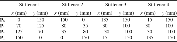
A sketch of the configurations is presented in Fig. 2, where the stiffener paths, boundary and loading conditions are illustrated.
Test cases: (a) Configuration C1 under bi-axial load; (b) Configuration C2 under bi-axial load; (c) Configuration C3 under bi-axial load; (d) Configuration C3 under bi-axial and shear load.

3.1 Configuration C1: bi-axial load
The first example deals with the post-buckling response of configuration C1 under bi-axial loading conditions. The edges
 $x = \pm a/2$
are loaded with a membrane force, whereas the transverse displacement is set to zero at
 $y = \pm b/2$
. The out-of-plane deflection is prevented on all four edges. The sketch of the panel is reported in Fig. 2(a), together with the loading and boundary conditions.
A preliminary convergence analysis is carried out to identify the number of functions to guarantee the convergence of the results. The analyses are conducted with the asymptotic-numerical method and the Newton-Raphson routine. For the former, the results are presented by considering both the pure displacement and the pseudo-mixed formulation.
In this context, the analyses with increasing number of trial functions are interrupted when the load parameter
 $\lambda $
is equal to 13. This stopping condition is meant to maintain the same load level for all the analyses, thus allowing to compare the results in terms of the out-of-plane displacement. Furthermore, the specific choice of
 $\lambda = 13$
is coherent with the unrestricted terminal condition returned from each analysis. The order of the perturbation expansion is
 $10$
, and the parameter
 $\epsilon $
is equal to
 ${10^{ - 5}}$
. The continuation procedure is conducted by considering
 $10$
steps. In addition a correction is added to the procedure, and iterations are carried out until a convergence criterion is met.
The results of the numerical tests are summarised in Table 3 in terms of buckling multiplier,
 ${\lambda _{cr}}$
, maximum out-of-plane deflection,
 ${w_{max}}$
, and CPU time,
 ${t_{CPU}}$
. The results are computed by considering the pure displacement approach,
 $AN{M_{disp}}$
, and the pseudo-mixed one,
 $AN{M_{mix}}$
. The CPU time is reported in nondimensional form by considering the Newton-Raphson,
 $NR$
, procedure with
 $R = S = 20$
as a reference.
As seen in Table 3, the buckling multiplier
 ${\lambda _{cr}}$
is captured with a good degree of accuracy with as few as
 $R = S = 5$
functions. However, this choice corresponds to a noticeable underestimation of the the maximum out-of-plane displacement with respect to the converged one. When the number of functions is increased to
 $R = S = 15$
, the predictions are found to be satisfactory in terms of buckling multiplier and post-buckling deflection, too.
The results of Table 3 clearly illustrate the advantages offered by the ANM method. In particular, the advantage over the Newton-Raphson approach increases with the number of functions. For instance, when
 $R = S = 20$
, the asymptotic-numerical method requires about one third of the time employed by Newton-Raphson. The results of Table 3 are useful for comparing the different times required by the displacement and pseudo-mixed ANM approaches. In particular, the advantage of the pseudo-mixed formulation is clear when a relatively large number of trial functions is considered. The maximum gain is 15% approximately, and corresponds to the case
 $R = S = 20$
. In spite of this moderate time saving, the pseudo-mixed formulation is more complex to be implemented when the compatibility between the skin and the stiffener needs to be imposed. For this reason, the displacement formulation is retained next.
To shed light into the influence of the ANM parameters on the solution, a sensitivity analysis is carried out. The expansion order, the number of steps and the parameter
 $\epsilon $
are varied, while the number of trial functions is fixed at
 $20$
. No stopping condition is imposed on the load parameter
 $\lambda $
in this case, so all the solutions are terminated at the end of the selected load steps. The results are summarised in Table 4.
Configuration C1: comparison in terms of linearised buckling parameter, load parameter, maximum out-of-plane deflection and CPU time between ANM and NR (Pert. exp. order = 10,
 $\epsilon = {10^{ - 5}}$
, Steps = 10)

 ${{\rm{\;}}^{\rm{a}}}{{\boldsymbol{t}}_{ref}}$
is the time employed by NR with R = S = 20 and 100 incremental steps.
Sensitivity analysis for configuration C1: comparison in terms of load parameter, maximum out-of-plane deflection and CPU time for ANM (R = S = 20)

 ${{\rm{\;}}^{\rm{a}}}{{\boldsymbol{t}}_{ref}}$
is the time employed by NR with R = S = 20 and 100 incremental steps.
By increasing the order of the perturbation expansion, the solution can move further along the equilibrium path with the same number of steps, as seen by the larger value of
 $\lambda $
. The same conclusion is drawn for the number of load steps. The parameter
 $\epsilon $
is decreased up to
 $\epsilon = {10^{ - 7}}$
. The result is a reduction of the final load parameter, meaning that a smaller part of the equilibrium path is captured.
The equilibrium path obtained with the asymptotic-numerical method and Newton-Raphson is illustrated in Fig. 3 in terms of maximum out-of-plane displacement against the load parameter. The number of trial functions is set to
 $R = S = 20$
, while all the relevant parameters of the asymptotic-numerical method are those employed to conduct the analysis in Table 3 and are kept unchanged in the subsequent analyses, unless otherwise stated. Figure 3 shows the force-displacement curve with and without a correction procedure in the ANM.
Force-displacement curve for configuration C1: (a) without correction; (b) with correction.

As seen from Fig. 3(a), when a correction procedure is not carried out, the two curves present a gap, which gets wider as the load increases, illustrating a drift of the solution. In Fig. 3(b), a correction procedure is included in the asymptotic routine: the force-displacement curve obtained with the asymptotic-numerical method closely matches the one obtained with Newton-Raphson.
3.2 Configuration C2: bi-axial load
To further assess the potential of the proposed approach, the configuration C2 is analysed. The panel is now characterised by the presence of two stiffeners and is subjected to the same boundary and loading conditions of the previous example. The sketch is provided in Fig. 2(b).
The results are validated against Abaqus finite element simulations. The models are realised with S4R elements, 4-node shell elements with reduced integration for the skin, and B31 elements, 2-node shear deformable beam elements for the stiffeners. The converged mesh corresponds to 3,720 elements and 3,721 nodes. In the models, the fiber angle is constant for each element and equal to the orientation evaluated at the element centroid. The contour of the out-of-plane displacement and the membrane resultants at
 $\lambda /{\lambda _{cr}} = 4.42$
are reported in Fig. 4. The plots illustrate the comparison against the Abaqus simulations.
Out-of-plane deflections and membrane resultants for configuration C2: (a)–(d) Ritz asymptotic-numerical method; (e)–(h) Abaqus.

The post-buckled shape is of global type as the stiffeners undergo bending deformations. One can appreciate the accuracy of the developed method in appropriately capturing not only the post-buckling shape, but also the membrane resultants distribution. In particular, the membrane resultant
 ${N_{xx}}$
redistribution towards the edges, typical of the post-buckling response of axially loaded plates, is clearly visible in Fig. 4(b) and (f). The maximum out-of-plane deflection is reported in Fig. 5, where ANM and Abaqus results are compared.
Force-displacement curve for configuration C2.

As seen, the curves are very similar, further validating the accuracy of the predictions via Ritz-ANM method.
For what concerns the computational time, the ANM method requires one third of the time required by a Newton-Raphson scheme. When compared with a FE-based strategy, extra time saving is achieved due to a much faster modeling phase, where no mesh is required.
3.3 Configuration C3: bi-axial load
The third example aims at illustrating the capabilities of the method to deal with more complex configurations, i.e. panels stiffened by curvilinear stringers. The structure is loaded and constrained as illustrated in Fig. 2(c). To verify the accuracy of the post-buckling response, the results are checked against simulations based on the Newton-Raphson procedure, this approach being validated in a previous study [Reference Vescovini and Foligno29]. The number of steps is varied to verify the quality of the solution at different load levels. The contour of the out-of-plane displacement is reported in Fig. 6.
Out-of-plane deflections at different load levels for configuration C3: (a)–(d) Asymptotic-numerical method; (e)–(h) Newton-Raphson.

At each load level, the contours in Fig. 6 reveal an excellent degree of agreement between ANM and NR predictions. The response is characterised by a post-buckled shape with two halfwaves in the longitudinal direction. The deflected pattern experiences a progressive change of shape as the load level increases. The complexity of the pattern provides good evidence of the ability of the method to precisely capture the panel response in the post-buckling regime.
The contour of the membrane resultants at
 $\lambda /{\lambda _{cr}} = 3.68$
is illustrated in Fig. 7. Even in this case, the distribution of the membrane forces is accurately predicted. The presence of both non-linear fibers distribution and curvilinear stiffeners is responsible for a relatively complex stress distribution. The membrane resultants present the typical redistribution mechanism toward the edges; as opposed to the case of straight stiffeners, here the presence of the stringers provides further load-carrying capabilities, causing peaks in the
 ${N_{xx}}$
resultant pattern. As seen in Fig. 8, the equilibrium path obtained with the perturbation technique closely matches the one obtained with Newton-Raphson.
Membrane resultants for configuration C3 at
 $\lambda /{\lambda _{cr}} = 3.68$
: (a)–(c) Asymptotic-numerical method; (d)–(f) Newton-Raphson.

Force-displacement curve for configuration C3.

The presence of the stiffeners does not increase the number of degrees of freedom, therefore the computational time for the analyses is similar to the first example. The evaluation of the stiffeners strain energy requires additional line integrals to be performed. However, this operation requires just a slight increase in the number of operations. Even in this case, the time saved for the different analyses is roughly 70
 ${\rm{\% }}$
with respect to NR routines.
3.4 Configuration C3: bi-axial and shear load
The last example is introduced to illustrate a more complex loading scenario, where bi-axial and shear loads are applied in combination, as shown Fig. 2(d). The ratio between the two loads is defined as
 $\gamma = {N^{shear}}/{N^{bi-axial}}$
. The results are presented for
 $\gamma = 0.5$
,
 $\gamma = 1$
and
 $\gamma = 2$
. The number of load steps is set to 20, resulting in different load levels for the three test cases: specifically,
 $\lambda /{\lambda _{cr}}$
is found to be equal to 3.97, 3.92 and 4.62 for
 $\gamma $
equal to 0.5, 1 and 2, respectively. The boundary conditions are the same of the previous example. The in-plane and out-of-plane displacement components are shown in Fig. 9.
In-plane displacements and out-of-plane deflection for configuration C3 with different ratios of bi-axial and shear loads: (a)–(c)
 $\gamma = 0.5$
; (d)–(f)
 $\gamma = 1$
; (g)–(i)
 $\gamma = 2$
.

From Fig. 9(a) to (c), the similarity can be noted between the post-buckled shape for
 $\gamma = 0.5$
and the pure bi-axial one of Fig. 6; indeed, the contribution of the bi-axial load is more relevant. The responses obtained with
 $\gamma = 1$
and
 $\gamma = 2$
are more similar, meaning that also when the ratio between shear and bi-axial load is equal to
 $1$
, the contribution of the former is more significant. The in-plane displacements also vary with
 $\gamma $
, leading to a more complex distribution as the shear load contribution becomes bigger. The contours of the force resultants are depicted in Fig. 10 for the three ratios of
 $\gamma $
.
Membrane resultants for configuration C3 with different ratios of bi-axial and shear loads: (a)–(c)
 $\gamma = 0.5$
; (d)–(f)
 $\gamma = 1$
; (g)–(i)
 $\gamma = 2$
.

The
 ${N_{xx}}$
resultant redistribution towards the edges is more and more concentrated towards the stiffeners attaching points and presents higher peaks values as
 $\gamma $
increases. Also, the patterns of the transverse and the shear resultants varies accordingly, going from a bi-axial to a prevalent shear distribution.
In Fig. 11 the force-displacement curves are illustrated for the different loading conditions and compared to the ones obtained with the Newton-Raphson iterative-incremental routine. For
 $\gamma = 0.5$
, one can see a smoother curve similar to the one of the pure bi-axial case in Fig. 8. On the other hand, both curves with
 $\gamma = 1$
and
 $\gamma = 2$
feature a slope change given by the presence of the shear load. This slope change happens around
 $2.5$
times the critical load for
 $\gamma = 1$
and around
 $4$
times the critical load for
 $\gamma = 2$
. Nevertheless, in all cases the equilibrium path is correctly represented by the perturbation method as it is proven by the comparison with the Newton-Raphson results.
Force-displacement curves for configuration C3 with different ratios of
 $\gamma = \frac{{{N^{shear}}}}{{{N^{bi-axial}}}}.$

Considerations on time saving with respect to Newton-Raphson simulations are similar to the previous test cases. Again, a 70
 ${\rm{\% }}$
reduction of CPU time is observed.
4.0 Limitations
The proposed formulation is a viable mean for preliminary investigations on VS panels with curvilinear stiffeners. Indeed, it is particularly useful for performing preliminary studies in a short amount of time. Given its intrinsic purpose, the model suffers from some limitations. Firstly, the structure under investigation is a portion of a more complex structure. When referring to a typical aeronautical wing-box, the present model can be used to represent the upper or the lower cover between two ribs. In addition, the planform is rectangular and no curvature effects are introduced. Hence, the tapering of typical wing structures is not accounted for. The presence of cutouts is beyond the current modeling capabilities, too.
Restrictions exist in terms of loading and boundary conditions. The edges are assumed to be subjected to uniform boundary conditions, meaning that the same kinematic constraints are applied along the same edge. Likewise, the method is not able to handle loading regions involving only a portion of the edge.
The one-dimensional model for the stiffeners does not allow for local stringer instabilities to be captured, such as those involving the web or the flanges of blade, J and omega stringers. Even the interaction between the skin and the stringer is simplified if a beam model is adopted, as the exchange of internal forces is condensed upon a line rather than between the skin and the foot/flange of the stringer. At the same time, section deformability is not modeled. Nevertheless, the adoption of a beam model provides the enormous advantage of not requiring extra degrees of freedom, as the beam displacements are expressed as a function of the skin ones. More refined strategies could be implemented by modeling the stringer components as two-dimensional elements. Note, this strategy would involve a noticeable increase of the degrees of freedom, hence affecting the computational effectiveness of the approach. Even the intersection between stringers would require particular care.
5.0 Conclusions
A formulation for the post-buckling analysis of variable stiffness panels with curvilinear stiffeners is presented. The approach is developed combining the Ritz method for the spatial approximation, and the asymptotic-numerical method for solution of the non-linear governing equations. Three test cases are presented to validate the results against the ones obtained with the Newton-Raphson routine and Abaqus finite element simulations. The results illustrate an excellent degree of agreement with the aforementioned routines, demonstrating that the asymptotic-numerical method is a powerful solution strategy for determining the post-buckling response of innovative curvilinearly stiffened panels. For the unstiffened panel only, both a displacement-based formulation and a pseudo-mixed formulation are considered. The comparison between the two approaches shows that the pseudo-mixed formulation requires a lower computational time. Despite this, when dealing with stiffened panels, the pseudo-mixed formulation is not recommended, as it would require an increasing complexity in the enforcement of the compatibility between the stringers and the skin.
The proposed approach is promising for its high computational efficiency combined with almost null modelling time. Indeed, a Ritz-based model is particularly suitable for the analysis of curvilinearly stiffened structures, since node sharing between skin and stiffener is not needed as it would be in finite element simulations. The proposed formulation is a highly automated numerical method that does not require mesh generation. This is especially useful for optimisation procedures, as multiple configurations can be analysed without the need to regenerate the model. In addition, any potential difficulty arising from mesh distortion is fully avoided. Moreover, a much smaller number of degrees of freedom is employed with respect to finite element models with comparable accuracy, making the present method a valuable alternative.
The asymptotic-numerical method is particularly beneficial when the Ritz expansion is relatively large, such as in the case of 20 functions along both directions. This situation is relatively common in the design of curvilinearly stiffened panels, as local effects are generally relevant. In this context, the ANM offers a number of interesting features: lower computational time, larger range of validity of the solution and a complete analytic representation of the non-linear equilibrium path. For the test cases considered in this study, the proposed method demonstrates noticeable analysis time saving. The time required for the analysis is one third, approximately, of that required by an analogous incremental iterative Newton-Raphson approach.
Overall, the proposed method is a valuable alternative to standard finite elements and classical predictor-corrector techniques to perform preliminary analysis on variable stiffness panels with curvilinear stiffeners. Potential design advantages are not discussed here, but future activities will benefit from the proposed analysis method to better investigate this aspect.
Given the aforementioned limitations, the proposed strategy can be further extended by considering more complex panels configurations, i.e. shell-like panels with cutouts, and other thermo-mechanical loading conditions, such as prescribed displacements and temperature gradients. These developments are the topic of current research activities. The extension to a two-dimensional model for the stringers is another interesting subject to be addressed in future works.
Competing interests
The authors declare none.
Appendix
The linear and non-linear contributions of the strain vector
 ${\epsilon ^0}$
, of the matrix
 ${{\textbf{G}}_1}$
, of the plate forces and moments per unit length and of the matrices
 ${{\textbf{H}}_1}$
and
 ${{\hat{\textbf{H}}}_1}$
are detailed below:
 \begin{align}&\boldsymbol{\epsilon}^0_L =\begin{Bmatrix} u^0_{/x} + w^0_{/x} \, w^*_{/x}\\[5pt] v^0_{/y} + w^0_{/y} \, w^*_{/y}\\[5pt] u^0_{/y} + v^0_{/x} + w^0_{/x} w^*_{/y} + w^0_{/y} \, w^*_{/x}\end{Bmatrix}&\boldsymbol{\epsilon}^0_{NL} =\begin{Bmatrix} \frac{1}{2} ( w^0_{/x} )^2\\[5pt] \frac{1}{2} ( w^0_{/y} )^2\\[5pt] w^0_{/x} w^0_{/y}\end{Bmatrix}\end{align}
 \begin{align}&\textbf{G}_1^L =\begin{bmatrix}1\;\;\;\;\; & 0\;\;\;\;\; & 0\;\;\;\;\; & 0\;\;\;\;\; & \boldsymbol{\phi}_{w/x} \textbf{c}_w^*\;\;\;\;\; & 0\\[5pt] 0\;\;\;\;\; & 0\;\;\;\;\; & 0\;\;\;\;\; & 1\;\;\;\;\; & 0\;\;\;\;\; & \boldsymbol{\phi}_{w/y} \textbf{c}_w^*\\[5pt] 0\;\;\;\;\; & 1\;\;\;\;\; & 1\;\;\;\;\; & 0 &\boldsymbol{\phi}_{w/y} \textbf{c}_w^*\;\;\;\;\; & \boldsymbol{\phi}_{w/x} \textbf{c}_w^*\end{bmatrix}&\textbf{G}_1^{NL} (\textbf{c}) =\begin{bmatrix}0\;\;\;\;\; & 0\;\;\;\;\; & 0\;\;\;\;\; & 0\;\;\;\;\; & \boldsymbol{\phi}_{w/x} \textbf{c}_w\;\;\;\;\; & 0\\[5pt] 0\;\;\;\;\; & 0\;\;\;\;\; & 0\;\;\;\;\; & 0\;\;\;\;\; & 0\;\;\;\;\; & \boldsymbol{\phi}_{w/y} \textbf{c}_w\\[5pt] 0\;\;\;\;\; & 0\;\;\;\;\; & 0\;\;\;\;\; & 0 &\boldsymbol{\phi}_{w/y} \textbf{c}_w\;\;\;\;\; & \boldsymbol{\phi}_{w/x} \textbf{c}_w\end{bmatrix}\end{align}
 \begin{align}&\textbf{N}^L = \textbf{A} \: \boldsymbol{\epsilon}^0_L + \textbf{B} \: \textbf{k}&\textbf{N}^{NL} = \textbf{A} \: \boldsymbol{\epsilon}^0_{NL}\end{align}
 \begin{align}{{\textbf{M}}^{NL}} = {\textbf{B}}{\rm{\;}}\boldsymbol\epsilon _{NL}^0\end{align}
 \begin{align}&\textbf{H}_1^L =\begin{bmatrix}\frac{\textbf{t}^T}{J_s} \textbf{f}_u\;\;\;\;\; & \textbf{0}\\[5pt] \frac{\textbf{n}^T}{J_s} \textbf{f}_u\;\;\;\;\; & -\textbf{b}^T \boldsymbol{\mathcal{J}}^T \boldsymbol{\Phi}_{\varphi}\\[5pt] \frac{\textbf{b}^T}{J_s} \textbf{f}_u\;\;\;\;\; & \textbf{n}^T \boldsymbol{\mathcal{J}}^T \boldsymbol{\Phi}_{\varphi}\\[5pt] \textbf{0}\;\;\;\;\; & \frac{\textbf{t}^T}{J_s} \textbf{f}_{\varphi}\\[5pt] \textbf{0}\;\;\;\;\; & \frac{\textbf{n}^T}{J_s} \textbf{f}_{\varphi}\\[5pt] \textbf{0}\;\;\;\;\; & \frac{\textbf{b}^T}{J_s} \textbf{f}_{\varphi}\end{bmatrix}&\textbf{H}_1^{NL}(\textbf{c}) =\begin{bmatrix}\frac{\textbf{b}^T}{J_s} \textbf{f}_u \textbf{c}^u \, \textbf{f}_u\;\;\;\;\; & \textbf{0}\\[5pt] \textbf{0}\;\;\;\;\; & \textbf{0}\\[5pt] \textbf{0}\;\;\;\;\; & \textbf{0}\\[5pt] \textbf{0}\;\;\;\;\; & \textbf{0}\\[5pt] \textbf{0}\;\;\;\;\; & \textbf{0}\\[5pt] \textbf{0}\;\;\;\;\; & \textbf{0}\end{bmatrix}\end{align}
 \begin{align}&\boldsymbol{\hat{H}}_1^L =\begin{bmatrix}\frac{\textbf{t}^T}{J_s} \textbf{f}_u\;\;\;\;\; & \textbf{0}\\[5pt] \frac{\textbf{n}^T}{J_s} \textbf{f}_u\;\;\;\;\; & -\textbf{b}^T \boldsymbol{\mathcal{J}}^T \boldsymbol{\Phi}_{\varphi}\\[5pt] \frac{\textbf{b}^T}{J_s} \textbf{f}_u\;\;\;\;\; & \textbf{n}^T \boldsymbol{\mathcal{J}}^T \boldsymbol{\Phi}_{\varphi}\\[5pt] \textbf{0}\;\;\;\;\; & \frac{\textbf{t}^T}{J_s} \textbf{f}_{\varphi}\\[5pt] \textbf{0}\;\;\;\;\; & \frac{\textbf{n}^T}{J_s} \textbf{f}_{\varphi}\\[5pt] \textbf{0}\;\;\;\;\; & \frac{\textbf{b}^T}{J_s} \textbf{f}_{\varphi}\end{bmatrix}&\boldsymbol{\hat{H}}_1^{NL}(\textbf{c}) =\begin{bmatrix}\frac{1}{2} \frac{\textbf{b}^T}{J_s} \textbf{f}_u \textbf{c}^u \, \textbf{f}_u\;\;\;\;\; & \textbf{0}\\[5pt] \textbf{0}\;\;\;\;\; & \textbf{0}\\[5pt] \textbf{0}\;\;\;\;\; & \textbf{0}\\[5pt] \textbf{0}\;\;\;\;\; & \textbf{0}\\[5pt] \textbf{0}\;\;\;\;\; & \textbf{0}\\[5pt] \textbf{0}\;\;\;\;\; & \textbf{0}\end{bmatrix}\end{align}



