INTRODUCTION
A large number of experiments have been carried out during the last few decades to assess ammonia (NH3) loss on national scales in the EU (Velthof et al. Reference Velthof, Oudendag, Witzke, Asman, Klimont and Oenema2009). NH3 losses are also of major importance on the global scale and are related to the use of mineral N fertilizers (Zhuang & Wang Reference Zhuang and Wang2010), as well as the application and management of organic fertilizers (Saarijärvi & Virkajärvi Reference Saarijärvi and Virkajärvi2009; Sonneveld & Van den Akker Reference Sonneveld and Van Den Akker2011; Tran et al. Reference Tran, Vu, Sommer and Jensen2011). In addition to an economic loss due to reduced nitrogen utilization efficiency, NH3 emissions to the atmosphere also create environmental problems, such as soil degradation, eutrophication and air pollution (Dragosits et al. Reference Dragosits, Theobald, Place, Lord, Webb, Hill, ApSimon and Sutton2002; Sanderson et al. Reference Sanderson, Collins, Johnson and Derwent2006). Accurate assessment of NH3 loss is essential to support the development of regional and global emission factors and to identify best management strategies for reducing losses (Smith et al. Reference Smith, Gordon, Bourque, Campbell, Genermont, Rochette and Mkhabela2009). Furthermore, in situ determination of NH3 volatilization is expensive and time consuming (Wulf et al. Reference Wulf, Maeting and Clemens2002).
For fertilization with slurries, the highest NH3 fluxes generally occur immediately after slurry application and then decrease rapidly (Huijsmans et al. Reference Huijsmans, Hol and Hendriks2001). In a preliminary investigation of published field data of NH3 emissions after the application of slurry using different application methods and determined using different measurement techniques, it was found that cumulative emission after 24 h always exceeded 0·7 of total cumulative emission (Menzi et al. Reference Menzi, Katz, Fahrni, Neftel and Frick1998; Nyord et al. Reference Nyord, Sogaard, Hansen and Jensen2008). Thus, in the case of a close relationship, the duration of NH3 loss measurements could be reduced without significant loss of information. The aim of the present study was to investigate the relationship between total NH3 loss after several days of measurements with cumulative losses determined over different time intervals between initial slurry application and final NH3 sampling.
MATERIALS AND METHODS
Field experiment
Two multiple-plot field experiments were carried out in 2007 and 2008 on the Christian-Albrechts-University at Kiel Karkendamm (KD) (53°55′N, 9°56′E, 17 m a.s.l.) and Hohenschulen (HS) (54°18′N, 9°58′E, 32 m a.s.l.) farms located in the federal state of Schleswig-Holstein, Northern Germany. The field experiments included different canopy conditions (bare, cut rye grass, wheat with different growth stages and maize), and three types of slurries (pig, cattle or biogas slurry). Eight different N levels (0, 40, 60, 80, 100, 120, 140 and 180 kg N/ha) were tested. All treatment combinations were tested with four replicates. Experimental plots (12 × 12 m) were arranged without interspaces in rows consisting of 16 plots. Rows were separated by pathways 8 m wide. The total number of plots was 240 in HS and 96 in KD. Further details about the experiment design are available in Gericke et al. (Reference Gericke, Pacholski and Kage2011).
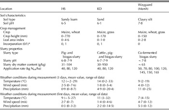
Data from another multi-plot field study carried out in the marsh area adjacent to the North Sea in northwest Germany and hereafter referred to as ‘Marsh’ (Quakernack et al. Reference Quakernack, Pacholski, Techow, Herrmann, Taube and Kage2011) were used to validate regression results. Compared to the field trials in KD and HS, wind speeds were higher and more regular in the Marsh trials. The soil in Marsh also had higher pH and higher clay content than the soils in KD and HS. Table 1 outlines soil, crop, weather and slurry characteristics information for the field experiments at the three sites.
Experimental conditions for NH3 loss measurement at three sites in the federal state of Schleswig-Holstein, Northern Germany, in the years 2007–10

* 1 and 0 represent with and without incorporation, respectively.
NH3 loss measurement method
The method is described in detail in Gericke et al. (Reference Gericke, Pacholski and Kage2011). In brief, NH3 emissions in the multi-plot field trials were measured by a combination of passive sampler measurements and measurements made with a dynamic chamber method, the Dräger Tube Method (DTM). The combined method is referred to as the calibrated passive sampling (CPS) method. Passive samplers were installed 0·15 m above the soil surface or crop canopy to capture NH3 emissions on the replicate plots (each measuring 12 × 12 m). For the duration of the trial, sample solution in the passive samplers was exchanged after 3–6 h during the day time and after c. 12 h following night-time sampling. NH3 concentration in the passive samplers was converted into absolute fluxes by using transfer coefficients (Vandre & Kaupenjohann Reference Vandre and Kaupenjohann1998) and in the present study these were obtained by the DTM (Pacholski et al. Reference Pacholski, Cai, Nieder, Richter, Fan, Zhu and Roelcke2006), which allows quantitative NH3-loss measurements on small plots in a relatively short time (c. 5 min). NH3 losses were determined 2–6 times a day, depending on the intensity of the volatilization process and for 1–4 days according to NH3 emission strength or until NH3 flux was negligible. Measurements with the DTM were made simultaneously with the passive sampling in 1 or 2 plots. Transfer coefficients were derived by relating the final cumulated NH3 losses determined by the DTM to cumulated NH3 uptake by passive samplers at the end of a measurement campaign (Gericke et al. Reference Gericke, Pacholski and Kage2011). Each treatment combination was measured on four replicate plots by CPS. Measurement data from each separate plot were used for model development.
In addition, a micrometeorological, backwards Lagrangian stochastic dispersion method (BLM; Sommer et al. Reference Sommer, McGinn and Flesch2005) was employed to measure NH3 emissions after the application of organic slurries to a large plot (40 × 40 m) in a field adjacent to the multi-plot field trial. Concentrations of NH3 in the atmosphere were determined by ‘Space Shuttle’ passive flux sampling (Leuning et al. Reference Leuning, Freney, Denmead and Simpson1985). Samplers were exchanged after 3–6 h during the day and after c. 12 h for night time sampling. NH3 fluxes were calculated by the backwards Lagrangian stochastic dispersion procedure implemented in the WindTrax-Software® (Thunderbeach Scientific, Halifax, Canada). The data obtained from BLM were used to check the results obtained from the multi-plot field study. Details of the NH3 emission measurement method and the good match between BLM and CPS are presented in Gericke et al. (Reference Gericke, Pacholski and Kage2011).
In total, 15 experimental campaigns in 2007 and 2008, and nine experiments in the Marsh region were used for linear model fitting and evaluation.
Definitions of variables
Variables used in the present investigation were defined as follows:
• cumloss f is the final measured cumulative NH3 loss at the end of measurements.
• sequence m is a particular subset of samplings (starting from 1) in the total sequence of measurements.
• cumloss m is cumulative NH3 loss after m hours.
• cumtime m is a specific cumulative time after sequence m.
Linear model fitting and testing
Model development was based on CPS measurements. However, as NH3 loss dynamics can be biased by the chosen measurement technique, the relationship between final NH3 losses and intermediate cumulated losses was tested by two additional measurement approaches, DTM and BLM. As the transfer coefficient for the calculation of absolute losses by CPS was obtained from final cumulated losses of the DTM, the NH3 loss dynamics studied by the former was independent of the calibration method used and a characteristic of the mere passive sampling.
The procedure for derivation and testing of the relationship between intermediate and final cumulated NH3 losses was as follows:
(1) Data from HS and KD by the method of CPS were used to study the relationship between cumloss f and cumloss m after sequence m. Linear model fitting was carried out and adjusted R 2 represents the goodness of fit.
(2) After identification of an optimal sequence m, a specific subset of samplings with a closely defined time interval was selected for model development. Data measured in 2007 were selected for parameterization of the linear model, and data obtained in 2008 and the Marsh as well as results obtained by DTM and BLM were used for validation.
(3) Parameter and model uncertainty of the linear model fit was evaluated by calculation of confidence and prediction intervals (Geisser Reference Geisser1993). The prediction interval quantifying the model uncertainty was also used to evaluate the prediction power of the model. Observed data located in the prediction interval are considered as a good match between model and data.
(4) The performance of the linear model was assessed for both parameterization and validation datasets by root mean square error (RMSE), mean bias error (MBE) and relative root mean square error (rRMSE), which were calculated by comparing the fitted and calculated cumloss f (Kennedy & Neville Reference Kennedy and Neville1986). To assess the effect of model uncertainty on the accuracy of predicted values, calculated final losses of replicated measurements were compared to measured final losses of the same replicates by means of t test (P < 0·05). For lack of replicates in the other validation data, the year 2008 validation dataset was used for this analysis.
All above analysis procedures were done using the statistical software R (version 2.9.2, Venables et al. Reference Venables and Smith2009).
RESULTS
Relationship between cumloss f and cumtime
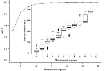
Distribution pattern of sequence m and the adjusted R 2 of linear model fitting are presented in Fig. 1. The adjusted R 2 increases rapidly with sequence m during the first hours of the measurements. At sequence 4 the adjusted R 2 exceeds 0·95, and the slope of the curve is very small after sequence 5. Although cumtime varied enormously, cumtime m for sequence 4 was always greater than 20 h and mostly close to 24 h (Fig. 1). In total, 203 of the 205 data records included cumtime 4 between 22 and 26 h after sequence 4. Therefore, cumulative NH3 losses for sequence 4 were chosen for further regression analysis to investigate the relationship between cumloss 24 and cumloss f.
Distribution pattern of cumtime and the adjusted R 2 of the linear model fitting between cumulative NH3 loss obtained by CPS from the start to each sequence m and cumloss f.

Regression analysis
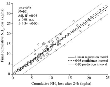
The regression analysis showed that cumulative NH3 losses after 24 h (sequence 4) had a very close linear relationship with final measured values (cumloss f) of the parameterization dataset (Fig. 2, n = 101). This relationship explained 0·94 of the variance of cumloss f, indicating that NH3 loss during the first 24 h accounted for approximately 0·75 of cumloss f due to a slope of 1·34. As the estimated intercept was not significant (P = 0·884), we re-estimated the simple linear regression without intercept to:
 $$\eqalign{cumloss_f {\rm (kg/ha)} = & \ {\rm 1} {\cdot} 34 \times cumloss_{24} \cr &{\ (R^{2} = 0{\cdot}98, P \lt 0{\cdot}001)}$$
A prediction using the linear model resulted in predicted values (Eqn 1) ±3·7 kg/ha (prediction interval).
Relationship between measured cumloss f (final cumulative NH3 loss) and cumloss 24 (cumulative NH3 loss during first 24 h). Data are from the measurement by the CPS method in HS and KD in 2007. Confidence interval (CI) and prediction interval (PI) are also presented.

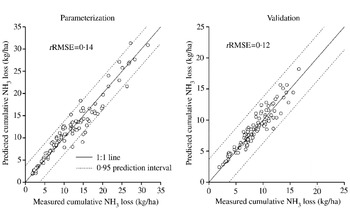
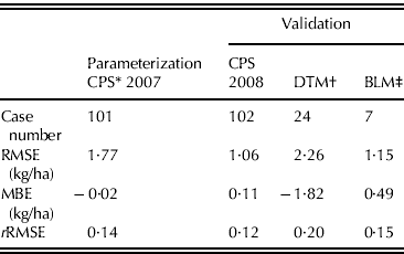
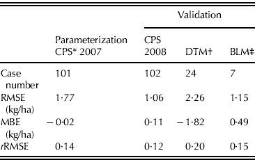
Sampling data measured in 2008 (n = 102) were employed to validate the prediction power of the above equation. The measured cumloss f fitted the linear equation obtained from parameterization well (Fig. 3). The rRMSE for parameterization and validation were 0·14 and 0·12, respectively (Fig. 3 and Table 2). The comparison of calculated and measured final losses of replicated measurements (n = 4) resulted in 25 out of 27 replicated measurements without significant difference (t test, P < 0·05). The two exceptions were due to heavy rainfall, untimely terminating the NH3 emission process.
Relationships between measured and predicted (Eqn 1) cumulative NH3 loss (cumloss f) in parameterization and validation. Parameterization data are from the measurement by CPS in HS and KD in 2007. Validation data are from the measurement by CPS in HS and KD in 2008. rRMSE is also presented for estimating the performance of the linear model prediction.

Evaluation of the empirical linear model's performance compared to different datasets at HS and KD
* CPS, calibrated passive sampling.
† DTM, Dräger tube method.
‡ BLM, backwards Langrangian stochastic dispersion method.
Validation by different measurement methods and study location
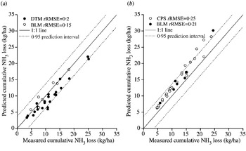
The relationships between prediction and observation for DTM and BLM at HS and KD are shown in Fig. 4a. The data points were distributed close to the one-to-one line for the BLM method and the RMSE and MBE were 1·15 and 0·49 kg/ha, respectively (Fig. 4a and Table 2). However, the calculated cumloss f was underestimated in DTM field measurements, with RMSE and MBE of 2·26 and −1·82 kg/ha, respectively. Stronger deviations in the DTM method were observed for medium or high emissions, while predictions for low emissions showed almost no differences. Nevertheless, the rRMSE for these two methods were not higher than 0·2 for the HS and KD sites (Table 2).
Comparison of measured and predicted (Eqn 1) cumulative NH3 loss (cumloss f) by the simple linear model using different datasets. (a) Data obtained by two different methods (BLM and CPS) in HS and KD during 2007 and 2008. (b) Data obtained from filed experiment performed in Waygarrd (marshland) during 2009 and 2010. rRMSE is also shown for estimating the performance of the linear model which derived from the linear model fitting of the data of CPS.

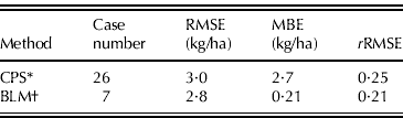
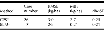
The simple linear model overestimated final NH3 emissions both for BLM and CPS in the Marsh study (Fig. 4b), which implies that the NH3 emission process was faster at this site or under the conditions that the field measurements were made. However, most observed records were still located in the prediction interval of the model (±3·7 kg/ha) (Fig. 4b). The RMSE for CPS and BLM were 3·0 and 2·8 kg/ha, respectively, and the rRMSE 0·25 in CPS and 0·21 in BLM (Table 3).
Evaluation of model performance in a marsh area in the years 2009/10
* CPS, calibrated passive sampling.
† BLM, backwards Lagrangian stochastic dispersion method.
DISCUSSION
Despite the large variation in final NH3 losses after different slurry application treatments at three sites in Northern Germany, good estimates of final losses could be obtained by a simple linear model using cumulative losses measured over 24 h. The relative deviation of calculated final losses for the sites KD and HS was less than 0·15 of cumloss f, which is the lowest level of measurement error in micrometeorological methods as reported by Harper & Sharpe (Reference Harper and Sharpe1998). A small effect of model uncertainty on the accuracy of predicted final losses as compared to measured final losses was shown by the statistical comparison between replicated predicted and measured final losses. The low rRMSE value in the parameterization was connected to a prediction uncertainty of 3·7 kg N/ha. This degree of uncertainty was achieved using a high number of data in the parameterization and could be attributed to high variation in NH3 loss data. The high intrinsic variation of replicated NH3 loss measurements after slurry application is due to uneven distribution of applied slurry, deviations from the target N application rate and variation in surface soil and canopy properties. The close agreement between calculated final losses by the simple linear model and the observations allows the conclusion that in spite of highly varying weather conditions, canopy, application levels and slurry types, total NH3 losses could be calculated with high confidence from measurements covering the first 24 h after application. Chantigny et al. (Reference Chantigny, Macdonald, Beaupre, Rochette, Angers, Masse and Parent2009) measured NH3 emissions from application of five types of treated liquid swine manure for 10 days and the results showed that cumulative NH3 loss during the first 24 h accounted for 0·60–0·80 of accumulated NH3 losses 3 days after application. Sanz et al. (Reference Sanz, Misselbrook, Sanz and Vallejo2010) used two micro-metrological techniques to measure NH3 emission from surface application of slurry and the results also showed that high NH3 emission rates lasted less than 20 h and cumulative NH3 loss during the first 24 h accounted for 0·70 of the final cumulative NH3 losses.
In the present study, NH3 emissions were determined on average for about 3 days until NH3 fluxes were undetectable or negligibly low. In some cases, however, NH3 emissions may last longer. Nevertheless, many studies have shown that NH3 emissions after slurry application were quantitatively negligible after 3 days of measurement, even under unfavourable conditions that might prolong the process of NH3 volatilization, e.g. low temperature (Misselbrook et al. Reference Misselbrook, Brookman, Smith, Cumby, Williams and Mccrory2005; Chantigny et al. Reference Chantigny, Macdonald, Beaupre, Rochette, Angers, Masse and Parent2009; Spirig et al. Reference Spirig, Flechard, Ammann and Neftel2010). According to laboratory work by Monaco et al. (Reference Monaco, Sacco, Pelissetti, Dinuccio, Balsari, Rostami and Grignani2012), c. 0·90 of fitted final total NH3 loss occurred during first 72 h. This has been tested on the present dataset by fitting a Michaelis–Menten-type saturation curve to the time courses of NH3 losses (Ni et al. Reference Ni, Pacholski, Gericke and Kage2011). The results showed that cumulative NH3 losses after the termination of measurements reached on average about 0·85 of the fitted asymptotic losses. However, estimated asymptotic losses can be considered as maximum values as possible environmental effects adverse to NH3 emissions after finishing the measurements (e.g. rainfall) cannot be considered in the curve fitting. Therefore, the slope of the regression curve might be slightly higher when using longer total measurement periods. However, the slope would probably lie within the prediction interval of the estimated function.
All the three NH3 volatilization measurement methods used were in close agreement regarding the NH3 loss dynamics. Model calculations showed slight underestimation for the DTM which may be due to the measurement procedure of this method. As the DTM is not a continuous measurement method, and only measures the flux rate during short time intervals and then integrates these finite flux rates into cumulative losses (Pacholski et al. Reference Pacholski, Cai, Nieder, Richter, Fan, Zhu and Roelcke2006), it is conceivable that some periods with high flux rates could be missed, particularly soon after slurry application. This was true for the present study, as it was not possible to measure on all plots simultaneously. Therefore, the model prediction showed better agreement with the time courses obtained with the DTM for low emissions, when initial emission rates were comparatively low (Fig. 4a), in particular with treatments with incorporated slurry which showed the lowest emissions. Nevertheless, notwithstanding the slight methodological bias, predictions of the final losses by the model (rRMSE 0·2, almost all data within the prediction interval) were very close to what is attainable on the background of variations of in situ NH3 loss data with deviation between replicates ⩾0·15 (Harper & Sharpe Reference Harper and Sharpe1998).
It should be noted that the present model was derived from experiments done on sites with wind speeds typical for non-coastal areas (average at 2 m height always <2 m/s). When validating the simple function with data obtained from the Marsh with higher wind speed and high soil pH, the model showed an overestimation. The implied high rate of the NH3 loss process can be both attributed to high wind speeds (Sommer et al. Reference Sommer, Olesen and Christensen1991) and high soil pH (Sommer & Ersboll Reference Sommer and Ersboll1996; He et al. Reference He, Alva, Calvert and Banks1999). However, deviations between model predictions and measured data were mainly within the prediction interval of the regression (Fig. 4b). The validation by data from the Marsh showed that a pronounced change of environmental conditions (i.e. wind speed) had a moderate effect on the slope of the linear model. Therefore, the presented model could be applied in this agro-landscape taking into account the given model uncertainty.
The present measurements as well as the analysed studies were carried out in temperate climate conditions and moderate temperatures (−2 to 33 °C). Compared to the present data, although measurements were carried out under a wide range of ambient temperatures (Table 1), climatic conditions with dominantly high temperatures can speed up the NH3 loss process (Sommer et al. Reference Sommer, Olesen and Christensen1991; Whitehead & Raistrick Reference Whitehead and Raistrick1991). Therefore, new regression studies would be required for hotter climates. In this case, where there is high uncertainty in the rate of the NH3 loss process, NH3 emission measurements from multiple plots could be simplified by calculating a new linear regression between final loss and intermediate cumulated losses from 1 to 2 plots. As a result, the slope of the linear relationship could be modified or the effective measurement time could differ from 24 h. Considering the variety of environmental conditions, measurements of final NH3 loss after slurry application should involve more than 2 days to derive a linear equation.
The datasets in the present study also included records related to slurry incorporation. Therefore, the linear model that was developed from slurry application by trailing hoses may be also applicable for other application methods. After analysis of field experiments conducted by Wulf et al. (Reference Wulf, Maeting and Clemens2002) with different application methods, reported cumloss 24 values accounted for 0·72 of cumloss f after harrowed application or injection of slurry on arable land. However, on grassland, cumloss 24 only accounted for 0·6 of cumloss f after injection of co-fermented cattle slurry. In the same study, cumloss 24 accounted for 0·82 of cumloss f after field application of animal slurries by trailing hose or splash plate. This strongly supports the application of an effective measurement time of 24 h, as in the present study.
The composition of organic slurries might have an effect on the slope of the regression function. The slurries tested in the present study (Table 1) covered a range of properties wider than the slurries used for the development of the ALFAM model (Sogaard et al. Reference Sogaard, Sommer, Hutchings, Huijsmans, Bussink and Nicholson2002), which is widely used for the simulation of NH3 emissions after slurry application. Therefore, the present linear model may be available to calculate NH3 loss from slurries with highly varying characteristics.
However, with respect to solid organic fertilizers (e.g. farmyard manure and composts) there different relationships probably exist between intermediate and final NH3 losses. McGinn & Sommer (Reference McGinn and Sommer2007) examined the NH3 emission from three types of cattle manure (fresh, composted and stored for 9 months) after application to a cropping soil. They detected NH3 emission 5 days after application of cattle manure that had been stored for 9 months. After applying composted cattle manure, NH3 emission did not commence until 2 days after application. The different NH3 emission pattern from solid manure may be attributed to its high dry matter content, which increases the residual time of manure on the soil surface, and its low water content, which hampers diffusion of NH4+ and NH3 through the manure matrix (Sogaard et al. Reference Sogaard, Sommer, Hutchings, Huijsmans, Bussink and Nicholson2002). Therefore, the relationship observed in the present study can only be applied to liquid manure applications.
In the present study, the prediction power of the linear model was evaluated by data from various NH3 measurement methods, liquid slurry and three different regions. However, a more extensive database on the effect of different application methods and soil/canopy conditions on NH3 losses is desirable to increase the accuracy of model predictions and to expand the linear model to a general use for all types and methods of slurry application. Nevertheless, under temperate climate conditions, the present findings strongly point to the opportunity to reduce the observation time for NH3 losses after field application of slurries by trail hoses and probably also other application methods to c. 24 h without significant information loss. The results showed that variation of environmental factors can change the slope of the linear model, but the model output was still valid under the given model uncertainty and variation in measured data. For a higher prediction accuracy in particular field trials or for NH3 emission measurements conducted under strongly differing conditions (e.g. hot weather and solid organic fertilizer), a new regression analysis would be required to test the effective measurement time and to parameterize the slope value.
The project was funded by the EU Regional Programme 2000 and the Ministry of Economy and Science of the Federal State of Schleswig-Holstein in the scope of the joint research project ‘Biogas-Expert’ as part of the ‘Schleswig-Holstein Center of Competence for the Use of Biomass’. Many thanks to Mr Robert Quakernack for supplying data from the Marsh experimental site. We are very grateful to Dr Deborah Turner, research fellow at the University of Melbourne, for revising the English writing of this manuscript.