1 Introduction
The stability of a shear layer in the presence of buoyancy forces is a classic problem in fluid mechanics, which was first considered by Taylor (Reference Taylor1931) and Goldstein (Reference Goldstein1931), and has applications in many areas, including industrial flows, atmospheric flows, astrophysical flows or, for example, in oceanography, where density gradients can be produced by variations in temperature or salinity, and mean flows can be created by wind, tides, etc. Often, the fluid is stably stratified, i.e. its density increases monotonically with depth. Such a fluid may be set in motion with a flow that is predominantly in a horizontal direction. If the flow is unstable, then it may become turbulent, which would enhance mixing of fluid from different depths, thus increasing the vertical transport of heat and other quantities of interest in modelling ocean dynamics. However, in this paper, rather than focus on a particular application, we consider uniform shear with simple density profiles that exhibit extraordinarily complicated sets of neutral stability curves, which, nonetheless, may have a corresponding behaviour in a variety of applications.
In some parameter planes the neutral curves form fractal sets, and one of the parameters that can reveal the fractal behaviour is the wave angle. Squire’s theorem was extended to stratified flows by Yih (Reference Yih1955), and shows how the stability of a three-dimensional wave corresponds to the stability of a two-dimensional wave in a flow with stronger stratification. In cases where stratification is destabilizing, this can lead to the most unstable wave being three-dimensional; Smyth & Peltier (Reference Smyth and Peltier1990) give an example of such a flow. The same is true in some flows considered here.
A bulk Richardson number,
 $J_{B}$
, (defined below) characterizes the strength of buoyancy effects compared to shear for a flow, and is fixed in a given experiment on the stability of some steady basic flow (in this paper, ‘experiment’ could refer to either a physical flow or to a numerical experiment based on simulation). Our approach will be to obtain stability results for two-dimensional waves for a range of
 $J_{B}$
, and to use the generalization of Squire’s theorem to show how the results would apply to an experiment at a fixed
 $J_{B}$
where waves of all wave angles may be present.
The problem to be solved is presented in § 2. Essentially we consider flows where
 $N_{\ast }^{2}=-g\bar{\unicode[STIX]{x1D70C}}^{\prime }/\bar{\unicode[STIX]{x1D70C}}$
has a quadratic dependence on the vertical coordinate,
 $y$
, which is measured positive in a direction opposite to gravity, a prime indicates a
 $y$
-derivative,
 $g$
is acceleration due to gravity,
 $\bar{\unicode[STIX]{x1D70C}}=\bar{\unicode[STIX]{x1D70C}}(y)$
is the basic density profile and
 $N_{\ast }=N_{\ast }(y)$
is the dimensional Brunt–Väisälä frequency. Previous work on these flows, connections with more realistic geophysical flows, and motivations for our extension are also given. Numerical results presented in § 3 suggest fractal-like behaviour, and asymptotic results presented in § 4 confirm and elucidate these fractal properties in the appropriate limits. Conclusions are given in § 5.
2 Problem formulation and motivation
2.1 The stability equation
Consider waves proportional to
 $\exp \text{i}[\unicode[STIX]{x1D6FC}(x-ct)+\unicode[STIX]{x1D6FD}z]$
, where the basic flow,
 $U=U(y)$
, is in the
 $x$
direction. Neglecting viscosity, and diffusion of the density field, and linearizing about the basic state leads to the disturbance equation
 $$\begin{eqnarray}\displaystyle v^{\prime \prime }-\left[\frac{(\unicode[STIX]{x1D6FC}^{2}+\unicode[STIX]{x1D6FD}^{2})g\bar{\unicode[STIX]{x1D70C}}^{\prime }}{\unicode[STIX]{x1D6FC}^{2}\bar{\unicode[STIX]{x1D70C}}(U-c)^{2}}+\frac{U^{\prime \prime }}{U-c}+\unicode[STIX]{x1D6FC}^{2}+\unicode[STIX]{x1D6FD}^{2}\right]v=\frac{\bar{\unicode[STIX]{x1D70C}}^{\prime }}{\bar{\unicode[STIX]{x1D70C}}}\left(\frac{U^{\prime }v}{U-c}-v^{\prime }\right), & & \displaystyle\end{eqnarray}$$
where
 $v$
is the vertical component of the disturbance velocity, see Drazin & Reid (Reference Drazin and Reid1981). Application of homogeneous boundary conditions to
 $v$
gives an eigenvalue problem for
 $c$
. If
 $\text{Im}(c)>0$
for real
 $\unicode[STIX]{x1D6FC}$
and
 $\unicode[STIX]{x1D6FD}$
, the flow is unstable.
To facilitate discussion of previous work, without yet specifying
 $U$
or
 $\bar{\unicode[STIX]{x1D70C}}$
, let
 $u_{0}$
be a characteristic velocity,
 $h_{0}$
a characteristic length,
 $\unicode[STIX]{x1D70C}_{0}$
a characteristic density and
 $\unicode[STIX]{x0394}\unicode[STIX]{x1D70C}$
a characteristic change in density over the region of interest. A bulk Richardson number can be defined by
 $$\begin{eqnarray}\displaystyle J_{B}=\frac{\unicode[STIX]{x0394}\unicode[STIX]{x1D70C}gh_{0}}{\unicode[STIX]{x1D70C}_{0}u_{0}^{2}}, & & \displaystyle\end{eqnarray}$$
which is a dimensionless parameter characterizing the relative strengths of buoyancy and shear. The local Richardson number,
 $$\begin{eqnarray}\displaystyle Ri(y)=-\frac{g\bar{\unicode[STIX]{x1D70C}}^{\prime }}{\bar{\unicode[STIX]{x1D70C}}{U^{\prime }}^{2}}=\frac{N_{\ast }^{2}}{{U^{\prime }}^{2}}, & & \displaystyle\end{eqnarray}$$
is another dimensionless quantity comparing buoyancy effects to shear, but as a function of
 $y$
. Howard (Reference Howard1961) and Miles (Reference Miles1961) proved that a necessary condition for instability is that
 $Ri<1/4$
somewhere in the flow.
If
 $\unicode[STIX]{x0394}\unicode[STIX]{x1D70C}/\unicode[STIX]{x1D70C}_{0}$
is small, and
 $J_{B}=O(1)$
, then the Boussinesq approximation can be made in which the terms on the right-hand side of (2.1) are neglected, and the buoyancy term retained, thus reducing (2.1) to the dimensionless Taylor–Goldstein equation,
 $$\begin{eqnarray}\displaystyle v^{\prime \prime }+\left[\frac{J_{B}N^{2}}{(U-c)^{2}}-\frac{U^{\prime \prime }}{U-c}-\unicode[STIX]{x1D6FC}^{2}\right]v=0,\quad N^{2}=-\frac{h_{0}\bar{\unicode[STIX]{x1D70C}}^{\prime }}{\bar{\unicode[STIX]{x1D70C}}}=\frac{h_{0}N_{\ast }^{2}}{g}, & & \displaystyle\end{eqnarray}$$
for two-dimensional waves (
 $\unicode[STIX]{x1D6FD}=0$
), where
 $N(y)$
is a dimensionless Brunt–Väisälä frequency.
The numerical solution of (2.4) for arbitrary
 $U$
and
 $\bar{\unicode[STIX]{x1D70C}}$
profiles is straightforward, provided appropriate care is taken near any critical points,
 $y=y_{c}$
, where
 $U(y_{c})=c$
. However, we shall consider simple model profiles, convenient for analytical work, in the hope of uncovering behaviour that might nonetheless be reflected in a variety of flows encountered in practice. In particular, we are interested in flows that have multiple neutral curves and multiple bands of instability in parameter space.
Early analytical work, when numerical solutions were hard to obtain, typically focussed on identifying profiles for
 $U$
and
 $\bar{\unicode[STIX]{x1D70C}}$
that admitted exact solutions in special functions for certain real values of
 $c$
, e.g. Thorpe (Reference Thorpe1969). Unstable waves may exist for wavenumbers near those that give real
 $c$
. Of course, these restrictions on
 $U$
,
 $\bar{\unicode[STIX]{x1D70C}}$
and
 $c$
are no longer required given the availability of numerical solutions. Nonetheless, while numerical solutions may allow more and more neutral curves to be found, exact solutions and asymptotic solutions can be used to prove the existence of infinitely many neutral curves, and to investigate their properties.
2.2 Plane Couette flow with quadratic variation of
 $N^{2}$

Possibly the simplest model showing infinitely many instability bands is the case of plane Couette flow,
 $U=y$
, between parallel plates with
 $N^{2}=y^{2}$
, where the plates are equidistant from
 $y=0$
, which was presented by Høiland & Riis (Reference Høiland and Riis1968). They found infinitely many neutral curves with
 $c=0$
, and it can be seen from (2.4) that the coefficient of
 $v$
is then constant, giving solutions for
 $v$
in terms of trigonometric functions. Note the symmetry of the problem:
 $U$
is an odd function, and
 $N^{2}$
is an even function, and in consequence there is no preferred direction of propagation for growing or neutral waves. Neutral waves therefore either have
 $c=0$
, or form a pair with equal and opposite phase velocities. In addition to the
 $c=0$
neutral curves found by Høiland & Riis (Reference Høiland and Riis1968), Huppert (Reference Huppert1973) presented neutral waves with
 $c\neq 0$
obtained using solutions for arbitrary
 $\unicode[STIX]{x1D6FC}$
and
 $c$
in terms of Whittaker functions, thus completing the stability diagram. (Huppert’s neutral curves are presented in figure 2
a below.)
The same flow has been used as a convenient example for investigating instability mechanisms in stratified flow, which are not obvious in this case because the flow is stable for homogeneous fluid, and is destabilized by statically stable stratification. Lindzen & Barker (Reference Lindzen and Barker1985) showed that this flow is an example where instability can be related to the over-reflection of waves at a critical point. Baines & Mitsudera (Reference Baines and Mitsudera1994) provided an alternative physical mechanism for the instability based on resonances between modes associated with the region
 $-1\leqslant y\leqslant 0$
interacting with modes associated with the region
 $0\leqslant y\leqslant 1$
; these modes have opposite energies in the sense of Cairns (Reference Cairns1979), so their interaction produces instability.
Howard & Maslowe (Reference Howard and Maslowe1973) considered plane Couette flow with
 $N^{2}=1+a^{2}y^{2}$
for several values of the parameter
 $a$
. The term independent of
 $y$
was shown to have a stabilizing effect. There is now only a finite number of neutral curves, and they no longer extend to arbitrarily large wavenumbers. The parameter
 $a$
controls the relative importance of the constant and quadratic terms, and as
 $a$
increases the number of unstable bands in parameter space increases, and the maximum unstable wavenumber increases, leading to behaviour that approaches the purely quadratic case
 $N^{2}=y^{2}$
.
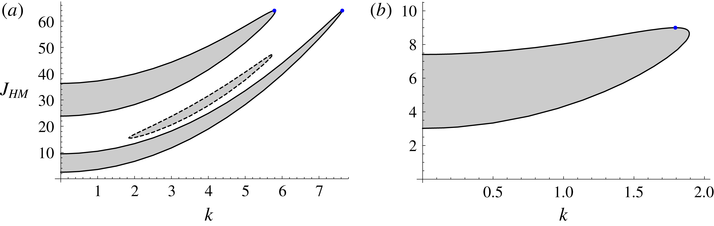
Instability diagrams for two-dimensional waves for (2.4) for cases studied by Howard & Maslowe (Reference Howard and Maslowe1973), i.e.
 $U=y$
and buoyancy profile (2.5). Shaded areas are unstable. Solid neutral curves have
 $c=0$
, and were presented in figure 4 of Howard & Maslowe (Reference Howard and Maslowe1973). The dashed neutral curve has
 $c\neq 0$
. The blue dots show points the minimum of the local Richardson number, which occurs at
 $y=0$
, is
 $1/4$
. (a) is for
 $a=16$
; (b) is for
 $a=6$
.

Instability diagrams for two-dimensional waves (
 $\unicode[STIX]{x1D719}=0$
) with
 $Ri_{0}=0$
. Shaded areas are unstable: (a) is for
 $y_{0}=0$
; (b) is for
 $y_{0}=0.2$
. Solid lines are neutral curves (3.4c
) along which
 $c=y_{0}$
; these are the same in both diagrams. Dashed lines are neutral curves along which
 $c\neq y_{0}$
.

In fact, Howard & Maslowe (Reference Howard and Maslowe1973) only presented neutral curves for
 $c=0$
, and for one of the cases they studied there is another band of unstable waves whose neutral curves have
 $c\neq 0$
. These modes are the continuation of Huppert’s
 $c\neq 0$
modes, and are shown in figure 1 for completeness. Howard & Maslowe’s buoyancy term can be written
 $$\begin{eqnarray}\displaystyle J_{B}N^{2}=J_{B}(1+a^{2}y^{2})=J_{HM}\left(\frac{1}{a^{2}}+y^{2}\right), & & \displaystyle\end{eqnarray}$$
where the second form corresponds more closely to the form (2.8) below that we will investigate in the present paper. The Miles–Howard theorem requires
 $Ri<1/4$
for instability, which is satisfied for this flow when
 $J_{HM}<a^{2}/4$
. The
 $c=0$
neutral curves touch this upper bound, but the
 $c\neq 0$
neutral curves are stabilized below this upper bound.
2.3 Similarities with geophysical flows
The flows described above, while convenient for analysis, and possibly even feasible for a laboratory experiment, might seem remote from flows typically observed in nature. However, there are qualitative similarities between the stability properties described above, and those of stratified mixing layers and boundary layers.
Miles (Reference Miles1963) found an infinite sequence of unstable bands in a rather artificial model of a mixing layer (chosen to facilitate solution in special functions). Miles’ model has the same symmetry as above:
 $U$
is an odd function, and
 $N^{2}$
is an even function, and again
 $c=0$
gives neutral curves. Many mixing layer studies have used models with the same symmetry. For example, Hazel (Reference Hazel1972) obtained numerical stability solutions for a mixing layer with
 $U=\tanh y$
and
 $N^{2}=\text{sech}^{2}(Ry)$
, which, for large enough
 $R$
, undergoes transitions between Kelvin–Helmholtz modes, which have
 $\text{Re}(c)=0$
, like those found by Høiland & Riis (Reference Høiland and Riis1968), and Holmboe modes, which have
 $\text{Re}(c)\neq 0$
, like those found by Huppert (Reference Huppert1973). In fact, Hazel’s flow also has arbitrarily many unstable bands, as shown by Alexakis (Reference Alexakis2005) (Hazel’s numerical study did not extend to large enough
 $J$
to observe multiple instability bands).
In practice, flows are not expected to be exactly symmetric. Even small symmetry breaking terms can act as singular perturbations, and produce qualitatively different behaviour. An immediate consequence is that
 $c=0$
is no longer a neutral curve, and the travelling waves no longer have equal and opposite phase velocities, as soon as symmetry breaking terms are introduced. There is a growing literature on asymmetric mixing layers, e.g. Hazel (Reference Hazel1972), Lawrence, Browand & Redekopp (Reference Lawrence, Browand and Redekopp1991), Lawrence, Haigh & Zhu (Reference Lawrence, Haigh and Zhu1998), Carpenter, Lawrence & Smyth (Reference Carpenter, Lawrence and Smyth2007), Carpenter, Balmforth & Lawrence (Reference Carpenter, Balmforth and Lawrence2010), which are more relevant to experiments and field observations.
Generally speaking, multiple bands of instability should be expected in flows with regions of strong stable stratification, provided there are also regions of weak stratification, where the local Richardson number,
 $Ri<1/4$
, somewhere in the flow. The solutions for
 $v$
are oscillatory in regions where the square bracket in (2.4) is positive. Chimonas (Reference Chimonas1974) uses this property to obtain sufficient conditions for instability for stratified flows without inflexion points. It is a simple extension to argue that as
 $J_{B}$
increases,
 $v$
oscillates over a shorter scale, and then more and more modes appear, which can be unstable if (2.3) still holds. Alexakis (Reference Alexakis2005) makes essentially the same argument by interpreting (2.4) as the Schrödinger equation with potential wells that deepen as
 $J_{B}$
increases. For example, Churilov (Reference Churilov2008) has shown that multiple instability bands occur for a stratified boundary layer flow as well.
In this paper we consider a generalization of the flows described in § 2.2, where an additional parameter is included that breaks the symmetry. This allows us to investigate the effect of asymmetry on flows with multiple instability bands. It can be anticipated that the number of neutral curves will increase because any pairs of neutral modes with equal and opposite phase velocities that exist in the symmetric case, will split apart when the flow becomes asymmetric, and will then have different phase velocities and growth rates.
2.4 Plane Couette flow with an asymmetric, quadratically varying
$N^{2}$

The dimensional profiles for our stably stratified plane Couette flow are
 $$\begin{eqnarray}\displaystyle U=u_{0}\frac{y}{h_{0}},\quad \bar{\unicode[STIX]{x1D70C}}=\unicode[STIX]{x1D70C}_{0}\left\{1-G^{-1}\left[Ri_{0}\frac{y}{h_{0}}+J\frac{(y-y_{0})^{3}}{3h_{0}^{3}}\right]\right\},\quad G=\frac{gh_{0}}{u_{0}^{2}},\quad & & \displaystyle\end{eqnarray}$$
where the plates lie at
 $y=\pm h_{0}$
, and move with velocities
 $\pm u_{0}$
relative to the midplane,
 $\unicode[STIX]{x1D70C}_{0}$
is a reference fluid density,
 $G$
is a dimensionless parameter describing the strength of acceleration due to gravity compared to the length and time scales associated with the shear flow and
 $Ri_{0}$
and
 $J$
are dimensionless parameters describing the density profile. The parameter
 $y_{0}$
gives the location of an inflexion point in the density profile, i.e. an extremum of the stratification, and, for
 $J>0$
,
 $y=y_{0}$
is where stratification is weakest. If
 $y_{0}=0$
we recover the symmetry of the plane Couette flows of § 2.2, and of the symmetric stratified mixing layers of § 2.3. Flows with
 $y_{0}\neq 0$
break this symmetry.
Introduce the following dimensionless variables, indicated by tildes,
 $$\begin{eqnarray}\displaystyle \tilde{v}({\tilde{y}})=\frac{v(y)}{u_{0}},\quad {\tilde{y}}=\frac{y}{h_{0}},\quad {\tilde{y}}_{0}=\frac{y_{0}}{h_{0}}, & & \displaystyle\end{eqnarray}$$
 $$\begin{eqnarray}\displaystyle \tilde{k}\cos \unicode[STIX]{x1D719}=\unicode[STIX]{x1D6FC}h_{0},\quad \tilde{k}\sin \unicode[STIX]{x1D719}=\unicode[STIX]{x1D6FD}h_{0},\quad \tilde{c}=\frac{c}{u_{0}}, & & \displaystyle\end{eqnarray}$$
where
 $\tilde{k}$
is the dimensionless magnitude of the wavevector and
 $|\unicode[STIX]{x1D719}|<\unicode[STIX]{x03C0}/2$
is the wave angle, with
 $\unicode[STIX]{x1D719}=0$
giving two-dimensional waves. Substitute (2.6) and (2.7) into (2.1), take
 $G\gg 1$
, which allows the Boussinesq approximation to be made, and drop the tildes, to give the dimensionless Taylor–Goldstein equation for profiles (2.6)
 $$\begin{eqnarray}\displaystyle v^{\prime \prime }+\left[\frac{N^{2}\sec ^{2}\unicode[STIX]{x1D719}}{(y-c)^{2}}-k^{2}\right]v=0,\quad N^{2}(y)=Ri(y)=Ri_{0}+J(y-y_{0})^{2}. & & \displaystyle\end{eqnarray}$$
Equation (2.8a
) is to be solved subject to
 $v(\pm 1)=0$
.
The minimum local Richardson number is
 $Ri_{0}$
, located at
 $y=y_{0}$
. A bulk Richardson number can be introduced based on the total change in density between the two plates, plate speed and plate separation as
 $$\begin{eqnarray}\displaystyle J_{B}=\frac{[\bar{\unicode[STIX]{x1D70C}}(-h_{0})-\bar{\unicode[STIX]{x1D70C}}(h_{0})]gh_{0}}{\unicode[STIX]{x1D70C}_{0}u_{0}^{2}}=2Ri_{0}+\frac{2}{3}(1+3y_{0}^{2})J & & \displaystyle\end{eqnarray}$$
using (2.6). The effect of considering an oblique wave with
 $\unicode[STIX]{x1D719}\neq 0$
is to increase
 $Ri_{0}$
and
 $J$
, and hence also
 $J_{B}$
, by a factor of
 $\sec ^{2}\unicode[STIX]{x1D719}$
relative to the two-dimensional case. Taking
 $Ri_{0}=y_{0}=0$
gives the case considered by Høiland & Riis (Reference Høiland and Riis1968) and Huppert (Reference Huppert1973). Taking
 $Ri_{0}\neq 0$
and
 $y_{0}=0$
gives the case considered by Howard & Maslowe (Reference Howard and Maslowe1973). Taking
 $y_{0}\neq 0$
breaks the even symmetry of
 $N^{2}$
.
3 Results suggesting fractal behaviour
In this section we present numerical solutions to (2.8) that seem to indicate the presence of a fractal structure to the neutral curves. Numerical solutions can only be used to examine a finite number of generations of the self-similar patterns. Certain features of these patterns are captured by perturbation theories, and these are presented too, confirming that the self-similar behaviour observed in the numerical solutions continues indefinitely to arbitrarily small scales, producing fractal behaviour. In § 4 higher-order perturbation theories are presented that give a more detailed description of the behaviour in the fractal limit beyond regimes accessible to numerical solutions.
The general solution to (2.8) can be expressed in terms of Whittaker functions,
 $$\begin{eqnarray}\displaystyle v=AM_{\unicode[STIX]{x1D705},\unicode[STIX]{x1D707}}(2\text{i}\sqrt{J\sec ^{2}\unicode[STIX]{x1D719}-k^{2}}[y-c])+BW_{\unicode[STIX]{x1D705},\unicode[STIX]{x1D707}}(2\text{i}\sqrt{J\sec ^{2}\unicode[STIX]{x1D719}-k^{2}}[y-c]), & & \displaystyle\end{eqnarray}$$
where
 $A$
and
 $B$
are arbitrary constants, and
 $$\begin{eqnarray}\displaystyle \unicode[STIX]{x1D705}=\frac{\text{i}(y_{0}-c)J\sec ^{2}\unicode[STIX]{x1D719}}{\sqrt{J\sec ^{2}\unicode[STIX]{x1D719}-k^{2}}}, & & \displaystyle\end{eqnarray}$$
 $$\begin{eqnarray}\displaystyle \unicode[STIX]{x1D707}=\sqrt{1/4-[Ri_{0}+J(y_{0}-c)^{2}]\sec ^{2}\unicode[STIX]{x1D719}}=\sqrt{1/4-Ri(y_{c})\sec ^{2}\unicode[STIX]{x1D719}}, & & \displaystyle\end{eqnarray}$$
see Olver et al. (Reference Olver, Lozier, Boisvert and Clark2010); the second form for
 $\unicode[STIX]{x1D707}$
follows from (2.8b
) and
 $y_{c}=c$
is the critical point. A solution satisfying
 $v(-1)=0$
is obtained by choosing
 $$\begin{eqnarray}\displaystyle A=W_{\unicode[STIX]{x1D705},\unicode[STIX]{x1D707}}(-2\text{i}\sqrt{J\sec ^{2}\unicode[STIX]{x1D719}-k^{2}}[1+c]),\quad B=-M_{\unicode[STIX]{x1D705},\unicode[STIX]{x1D707}}(-2\text{i}\sqrt{J\sec ^{2}\unicode[STIX]{x1D719}-k^{2}}[1+c]), & & \displaystyle \nonumber\\ \displaystyle & & \displaystyle\end{eqnarray}$$
and then the dispersion relation is obtained by substituting (3.3) into (3.1) and setting
 $v(1)=0$
. Note that the signs of the square roots in the above have been chosen corresponding to a solution path passing below
 $y_{c}$
in the complex
 $y$
plane, and this dispersion relation can be used to obtain regular roots with
 $\text{Im}(c)>0$
, singular neutral modes with
 $\text{Im}(c)=0$
, for which derivatives of
 $v$
are singular at
 $y_{c}$
when
 $Ri(y_{c})\neq 0$
, and also quasi-modes with
 $\text{Im}(c)<0$
, which are only defined along paths in the complex
 $y$
plane, but which are useful in describing solutions to inviscid initial value problems, and also damped viscous modes, see Briggs, Daugherty & Levy (Reference Briggs, Daugherty and Levy1970), Balmforth, Del-Castillo-Negrete & Young (Reference Balmforth, Del-Castillo-Negrete and Young1997), Shrira & Sazonov (Reference Shrira and Sazonov2001). We use this dispersion relation for the numerical evaluation of eigenvalues, but it does not offer easy insights into their dependence on parameters. For better understanding, we consider special cases and limits.
3.1 The special case
$Ri_{0}=0$

When
 $Ri_{0}=0$
, the trigonometric solutions, and neutral curves, for
 $c=0$
presented by Høiland & Riis (Reference Høiland and Riis1968), still exist in the asymmetric case of
 $y_{0}\neq 0$
, but now with
 $c=y_{0}$
. In this case (2.8) and its solutions are
 $$\begin{eqnarray}\displaystyle v^{\prime \prime }+(J\sec ^{2}\unicode[STIX]{x1D719}-k^{2})v=0,\quad v=\sin [n\unicode[STIX]{x03C0}(y+1)/2],\quad J=\cos ^{2}\unicode[STIX]{x1D719}\left(\frac{n^{2}\unicode[STIX]{x03C0}^{2}}{4}+k^{2}\right), & & \displaystyle \nonumber\\ \displaystyle & & \displaystyle\end{eqnarray}$$
for
 $n=1,2,3,\ldots \,$
. Note that the family of neutral curves (3.4c
) is independent of
 $y_{0}$
. However, the family of
 $c\neq y_{0}$
neutral curves do depend on
 $y_{0}$
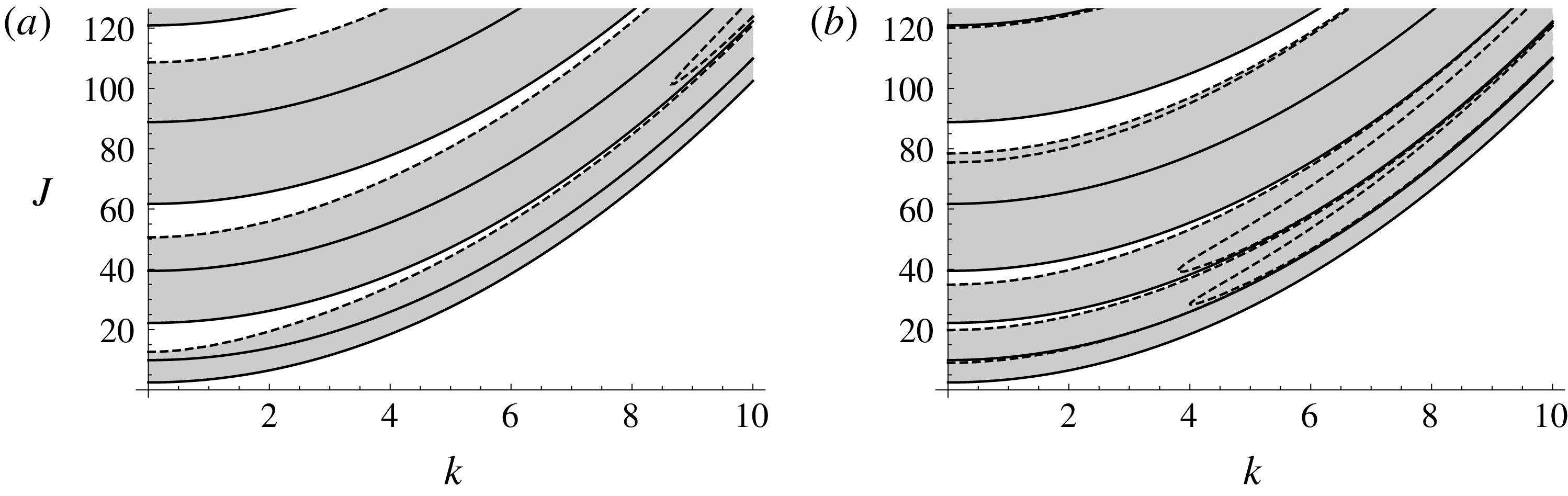
. Figure 2 shows the neutral curves and unstable regions for
 $y_{0}=0$
, which corresponds to figure 2 of Huppert (Reference Huppert1973), and for
 $y_{0}=0.2$
. In the symmetric case of
 $y_{0}=0$
,
 $\pm c$
pairs of
 $c\neq 0$
modes become unstable simultaneously, but when
 $y_{0}\neq 0$
this symmetry is broken, and each member of the pair becomes unstable at different parameter values, producing additional dashed neutral curves in figure 2(b) compared to figure 2(a).
At first sight, (3.4c
) seems to suggest that the effect of changing the wave angle is essentially trivial, in that it leaves the stability diagrams in figure 2 unchanged, except for a re-scaling of the vertical axis by a factor of
 $\cos ^{2}\unicode[STIX]{x1D719}$
. However, an experiment would be carried out at a particular value of
 $J$
, and waves of all wave angles would be present in a physical experiment. Therefore, instead of plotting
 $J$
against
 $k$
for a fixed
 $\unicode[STIX]{x1D719}$
, it may also be useful to present stability diagrams plotting
 $\unicode[STIX]{x1D719}$
against
 $k$
for a fixed
 $J$
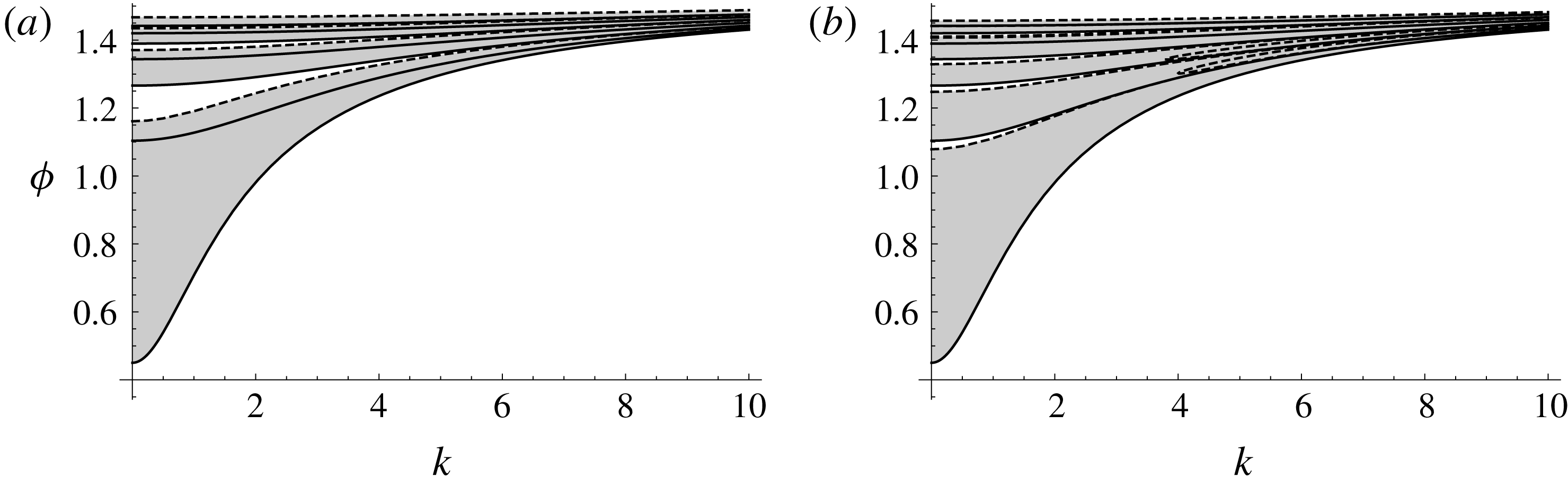
, as in figure 3.
Instability diagrams for
 $J=2$
and
 $Ri_{0}=0$
. Shaded areas are unstable: (a) is for
 $y_{0}=0$
; (b) is for
 $y_{0}=0.2$
. Solid lines are neutral curves (3.4c
) along which
 $c=y_{0}$
; these are the same in both diagrams. Dashed lines are neutral curves along which
 $c\neq y_{0}$
.

Two-dimensional waves are stable for
 $J<\unicode[STIX]{x03C0}^{2}/4$
according to (3.4c
), so for any
 $J$
in this range, as in figure 3, the lowest neutral curve intercepts the vertical axis at
 $\unicode[STIX]{x1D719}=\cos ^{-1}(2J^{1/2}/\unicode[STIX]{x03C0})$
(obtained from solving (3.4c
) for
 $\unicode[STIX]{x1D719}$
with
 $k=0$
and
 $n=1$
), and all waves with
 $|\unicode[STIX]{x1D719}|$
less than this value are stable. In this case, two-dimensional waves are stable, but three-dimensional waves are unstable. If
 $J>\unicode[STIX]{x03C0}^{2}/4$
, then two-dimensional waves are also unstable and the lowest neutral curve intercepts the horizontal axis at
 $k=\sqrt{J-\unicode[STIX]{x03C0}^{2}/4}$
(from solving (3.4c
) for
 $k$
with
 $\unicode[STIX]{x1D719}=0$
and
 $n=1$
).
While figure 2 shows that more and more two-dimensional waves become unstable as
 $J$
increases, i.e. as buoyancy effects become strong, figure 3 shows that even in a flow where buoyancy effects might be assumed to be negligible, buoyancy generates arbitrarily many unstable streamwise vortices with
 $\unicode[STIX]{x1D719}\rightarrow \unicode[STIX]{x03C0}/2$
in the inviscid limit. Thus even weak stray density gradients might destabilize streamwise vortices.
We now consider the dependence of the neutral curves on
 $y_{0}$
in more detail. Although the
 $c=y_{0}$
neutral curves (3.4c
) do not depend on
 $y_{0}$
, the growth and decay rates of modes adjacent to these neutral curves do depend on
 $y_{0}$
. The stability of these adjacent modes can be found using perturbation theory, which shows explicitly how the stability depends on both
 $k$
and
 $y_{0}$
for any integer value of
 $n$
.
Consider a small adjustment,
 $\unicode[STIX]{x1D716}$
, to the value of
 $J$
on the
 $n$
th neutral curve, and expand
 $v$
and
 $c$
in powers of
 $\unicode[STIX]{x1D716}$
,
 $$\begin{eqnarray}\displaystyle J=\cos ^{2}\unicode[STIX]{x1D719}\left(\frac{n^{2}\unicode[STIX]{x03C0}^{2}}{4}+k^{2}\right)+\unicode[STIX]{x1D716},\quad v=v_{0}+\unicode[STIX]{x1D716}v_{1}+\cdots \,,\quad c=y_{0}+\unicode[STIX]{x1D716}c_{1}+\cdots \,.\qquad & & \displaystyle\end{eqnarray}$$
Substitute (3.5) and
 $Ri_{0}=0$
into (2.8), expand for small
 $\unicode[STIX]{x1D716}$
, then equating coefficients of leading-order powers of
 $\unicode[STIX]{x1D716}$
gives
 $$\begin{eqnarray}\displaystyle & \displaystyle v_{0}^{\prime \prime }+\frac{n^{2}\unicode[STIX]{x03C0}^{2}}{4}v_{0}=0, & \displaystyle\end{eqnarray}$$
 $$\begin{eqnarray}\displaystyle & \displaystyle v_{1}^{\prime \prime }+\frac{n^{2}\unicode[STIX]{x03C0}^{2}}{4}v_{1}=-\left[\sec ^{2}\unicode[STIX]{x1D719}+\frac{(n^{2}\unicode[STIX]{x03C0}^{2}+4k^{2})c_{1}}{2(y-y_{0})}\right]v_{0}. & \displaystyle\end{eqnarray}$$
A solution to (3.6a
) satisfying
 $v_{0}=0$
at
 $y=\pm 1$
is
 $$\begin{eqnarray}\displaystyle v_{0}=\sin [n\unicode[STIX]{x03C0}(y+1)/2] & & \displaystyle\end{eqnarray}$$
for any positive integer
 $n$
. Equation (3.6a
) is self-adjoint, so multiplying (3.6b
) by
 $v_{0}$
, integrating the result from
 $y=-1$
to
 $y=1$
and imposing the homogeneous boundary conditions,
 $v_{1}=0$
at
 $y=\pm 1$
, gives the solvability condition
 $$\begin{eqnarray}\displaystyle \sec ^{2}\unicode[STIX]{x1D719}+\frac{(n^{2}\unicode[STIX]{x03C0}^{2}+4k^{2})c_{1}}{2}\int _{-1}^{1}\frac{\sin ^{2}[n\unicode[STIX]{x03C0}(y+1)/2]}{y-y_{0}}\,\text{d}y=0, & & \displaystyle\end{eqnarray}$$
where the integration path is taken into the complex
 $y$
plane below the pole at
 $y=y_{0}$
. The residue from this pole gives the stabilizing or destabilizing contribution from the critical point, and the imaginary part of the integral is
 $$\begin{eqnarray}\displaystyle \unicode[STIX]{x03C0}\sin ^{2}[n\unicode[STIX]{x03C0}(y_{0}+1)/2], & & \displaystyle\end{eqnarray}$$
which, in general, leads to a complex
 $c_{1}$
. The sign of
 $\text{Im}(c_{1})$
then determines whether the flow is stable or unstable for
 $J$
just above (
 $\unicode[STIX]{x1D716}>0$
), or just below (
 $\unicode[STIX]{x1D716}<0$
), its value on the neutral curve for a given
 $n$
.
However, for
 $n\geqslant 2$
there are certain values of
 $y_{0}$
for which (3.9) is zero, and then
 $c_{1}$
is real. In these cases, this leading-order perturbation theory does not determine the stability or instability of the waves near the neutral curve, and a higher-order theory is required (described in § 4.1 below). These special cases indicate parameter values where two or more neutral curves cross in the parameter plane. They occur when
 $$\begin{eqnarray}\displaystyle \frac{n\unicode[STIX]{x03C0}(y_{0}+1)}{2}=m\unicode[STIX]{x03C0}\quad \Rightarrow \quad y_{0}=\frac{2m-n}{n}, & & \displaystyle\end{eqnarray}$$
for any integer
 $m$
such that
 $-1<y_{0}<1$
, i.e.
 $1\leqslant m<n$
, so that the pole lies within the integration domain in (3.8).
A curious feature of (3.10b
), is that neutral curve crossings only occur when
 $y_{0}$
is rational, and they do not occur when
 $y_{0}$
is irrational.
In an experiment, distinctions between the rationality or irrationality of a measured distance, such as
 $y_{0}$
, must be irrelevant, as any distance is only known to within a finite precision. However, the presence of a crossing of neutral curves should be a robust feature of a stability diagram, and (3.10b
) shows that crossings occur each time
 $y_{0}$
changes by
 $2/n$
. Arbitrarily many crossings therefore occur as
 $y_{0}$
varies for large
 $n$
. Large
 $n$
modes correspond either to strong buoyancy (large
 $J$
) for two-dimensional waves, or for highly oblique waves (
 $\unicode[STIX]{x1D719}\rightarrow \unicode[STIX]{x03C0}/2$
) in an experiment at finite
 $J$
.
Figures 2 and 3 show neutral curves as a function of
 $k$
for fixed values of
 $y_{0}$
. We now consider neutral curves as a function of
 $y_{0}$
for fixed values of
 $k$
. In particular, we have selected
 $k=0$
as figures 2 and 3 show this value produces the lowest unstable
 $J$
for two-dimensional waves, and lowest unstable
 $\unicode[STIX]{x1D719}$
for fixed
 $J$
. In fact,
 $k=0$
is of more general interest because results for any fixed finite
 $k$
approach those for
 $k=0$
when either
 $J\rightarrow \infty$
or
 $\unicode[STIX]{x1D719}\rightarrow \unicode[STIX]{x03C0}/2$
.
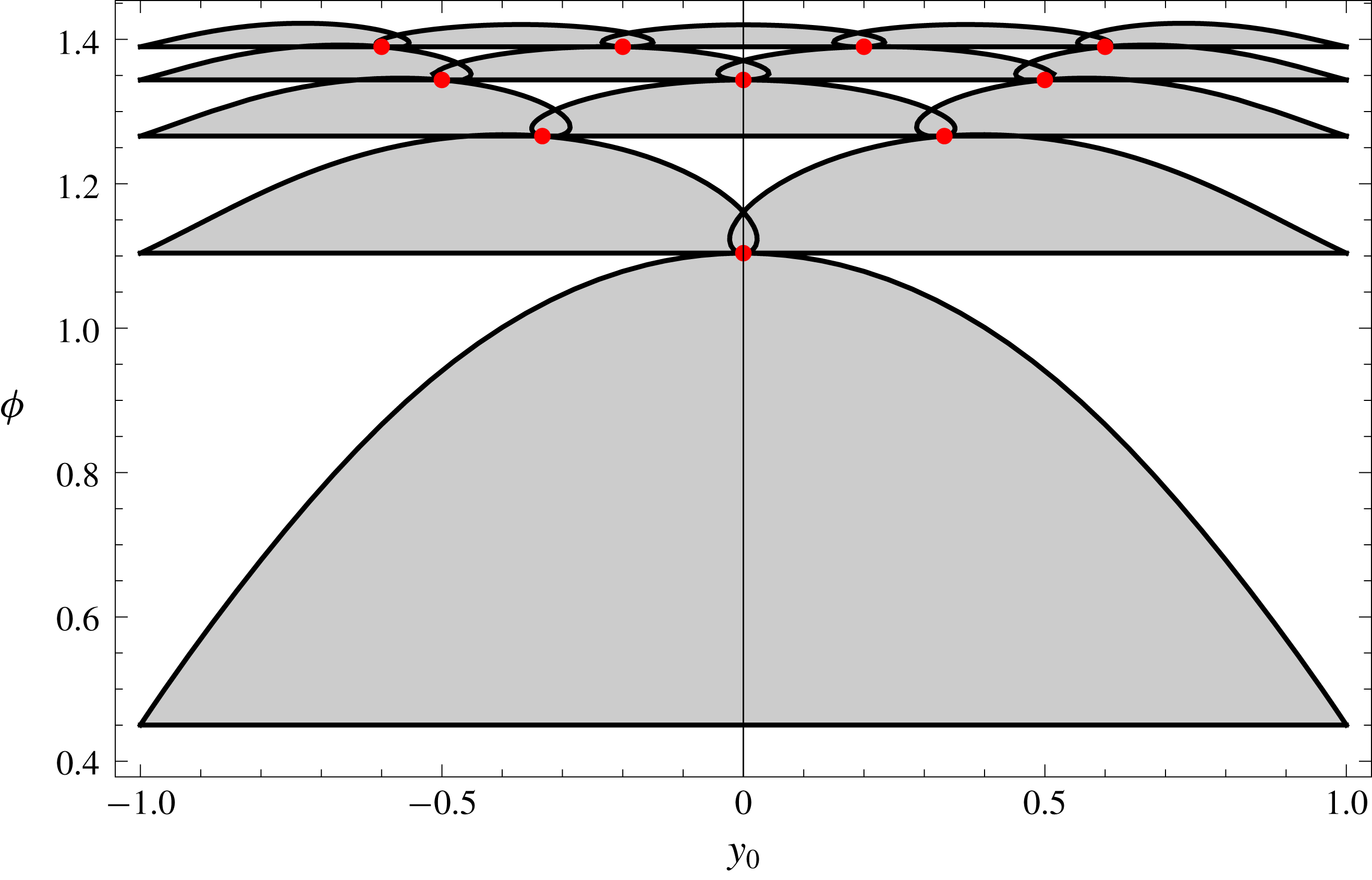
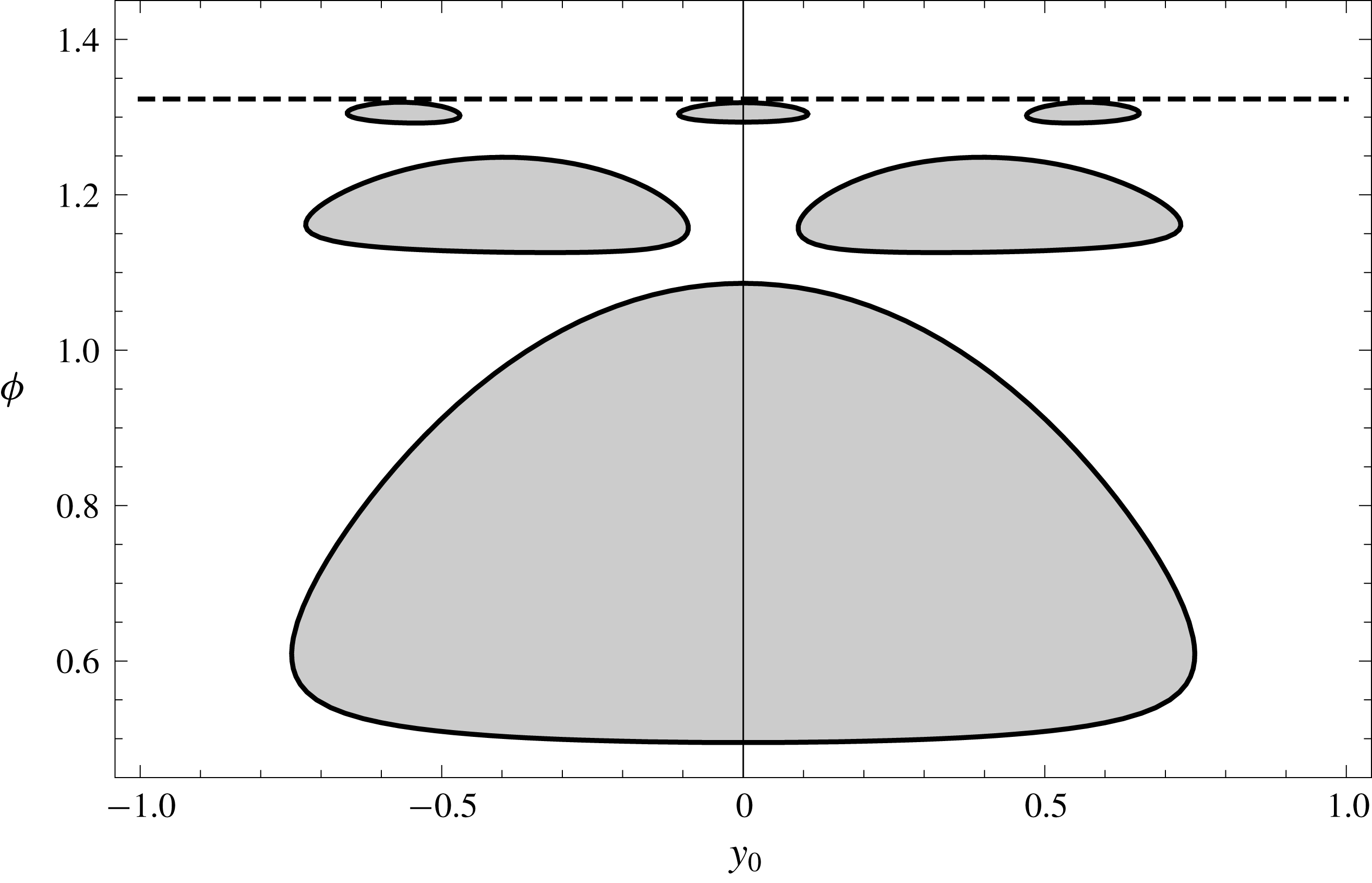
Figure 4 shows neutral curves obtained from numerical evaluation of the exact solutions (3.1). This numerical evidence suggests that three neutral curves cross at each red dot given by (3.10b ), with a larger unstable region below each red dot being joined to two smaller unstable regions above. The asymptotic behaviour near each red dot is analysed in detail in § 4. But here, instead of mapping out further unstable regions numerically, the underlying structure determined by the red dots is easily investigated by plotting just the red dots.
Instability diagram for
 $J=2$
,
 $Ri_{0}=0$
and
 $k=0$
. Shaded areas are unstable. Horizontal lines are the neutral curves (3.4c
) along which
 $c=y_{0}$
; along the curved portions of the neutral curves
 $c\neq y_{0}$
. The red dots are the points along the horizontal neutral curves given by (3.10b
).

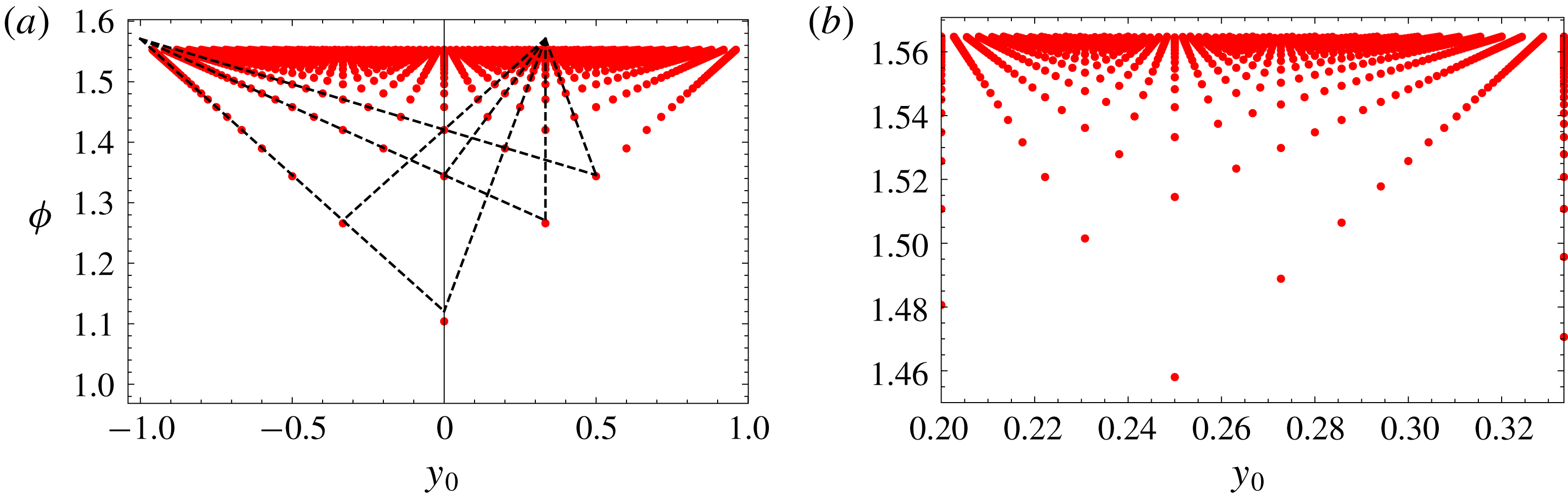
Figure 5 shows that the pattern of red dots produced by (3.10b
) has a self-similar structure repeating on smaller scales as
 $\unicode[STIX]{x1D719}\rightarrow \unicode[STIX]{x03C0}/2$
. This limit is reached as
 $n\rightarrow \infty$
, and then (3.4c
) gives
 $$\begin{eqnarray}\displaystyle \unicode[STIX]{x1D719}\sim \frac{\unicode[STIX]{x03C0}}{2}-\frac{2\sqrt{J}}{\unicode[STIX]{x03C0}n}+O(n^{-3}) & & \displaystyle\end{eqnarray}$$
for fixed finite
 $J$
and
 $k$
. Thus the pattern becomes independent of
 $k$
as
 $\unicode[STIX]{x1D719}\rightarrow \unicode[STIX]{x03C0}/2$
.
Distribution of points where neutral curves cross given by (3.4c
) and (3.10b
), as
 $n\rightarrow \infty$
for
 $J=2$
,
 $Ri_{0}=0$
and
 $k=0$
. (b) is a zoom of (a). Dashed lines in (a) show how points asymptote towards straight lines as
 $\unicode[STIX]{x1D719}\rightarrow \unicode[STIX]{x03C0}/2$
. The dashed lines radiating from
 $(y_{0},\unicode[STIX]{x1D719})=(-1,\unicode[STIX]{x03C0}/2)$
are obtained from (3.12a
) with
 $p=-1$
,
 $q=1$
and
 $r=1,2,3$
; the dashed lines radiating from
 $(y_{0},\unicode[STIX]{x1D719})=(1/3,\unicode[STIX]{x03C0}/2)$
are obtained from (3.12a
) with
 $p=1$
,
 $q=3$
and
 $r=-3,-2,-1,0,1$
.

Another striking feature is that, as
 $\unicode[STIX]{x1D719}\rightarrow \unicode[STIX]{x03C0}/2$
, the red dots lie on families of straight lines that radiate out from points at
 $(y_{0},\unicode[STIX]{x1D719})=(p/q,\unicode[STIX]{x03C0}/2)$
where the integers
 $p$
and
 $q$
have no common factors except 1 (
 $p$
and
 $q$
are relatively prime). The equations of the straight lines passing through
 $(y_{0},\unicode[STIX]{x1D719})=(p/q,\unicode[STIX]{x03C0}/2)$
are given by
 $$\begin{eqnarray}\displaystyle & \displaystyle \frac{\unicode[STIX]{x03C0}r}{q}\left(\unicode[STIX]{x1D719}-\frac{\unicode[STIX]{x03C0}}{2}\right)=-\sqrt{J}\left(y_{0}-\frac{p}{q}\right)\quad \text{for }p+q\text{ even}, & \displaystyle\end{eqnarray}$$
 $$\begin{eqnarray}\displaystyle & \displaystyle \frac{\unicode[STIX]{x03C0}r}{2q}\left(\unicode[STIX]{x1D719}-\frac{\unicode[STIX]{x03C0}}{2}\right)=-\sqrt{J}\left(y_{0}-\frac{p}{q}\right)\quad \text{for }p+q\text{ odd}, & \displaystyle\end{eqnarray}$$
 $r$
is an integer. The form for these equations can be verified by substituting (3.10b
) and (3.11) into (3.12). All the red dots in the limit
 $\unicode[STIX]{x1D719}\rightarrow \unicode[STIX]{x03C0}/2$
are generated by intersections between lines of the form (3.12) radiating from any pair of distinct points of the form
 $(p/q,\unicode[STIX]{x03C0}/2)$
.
Instability diagram for
 $J=2$
,
 $Ri_{0}=0.015$
and
 $k=0$
. Shaded areas are unstable. Horizontal dashed line is at
 $\unicode[STIX]{x1D719}=\cos ^{-1}(2\sqrt{Ri_{0}})$
. All waves above the dashed line are stable by the Miles–Howard theorem.

3.2 Cases with
$Ri_{0}\neq 0$

The fractal behaviour in figures 4 and 5 is truncated if
 $Ri_{0}\neq 0$
. The effective minimum local Richardson number for oblique waves is
 $Ri_{0}\sec ^{2}\unicode[STIX]{x1D719}$
, so all waves with
 $\cos ^{-1}(2\sqrt{Ri_{0}})\leqslant \unicode[STIX]{x1D719}\leqslant \unicode[STIX]{x03C0}/2$
are stable by the Miles–Howard theorem. Figure 6 presents an example of the finite number neutral curves for three-dimensional waves in a flow with a fixed
 $J$
and a non-zero
 $Ri_{0}$
. When
 $Ri_{0}$
is reduced, the dashed line in this figure moves upwards, revealing more and more neutral curves, and the unstable regions grow and approach one-another, until the fractal pattern shown in figure 4 appears at
 $Ri_{0}=0$
.
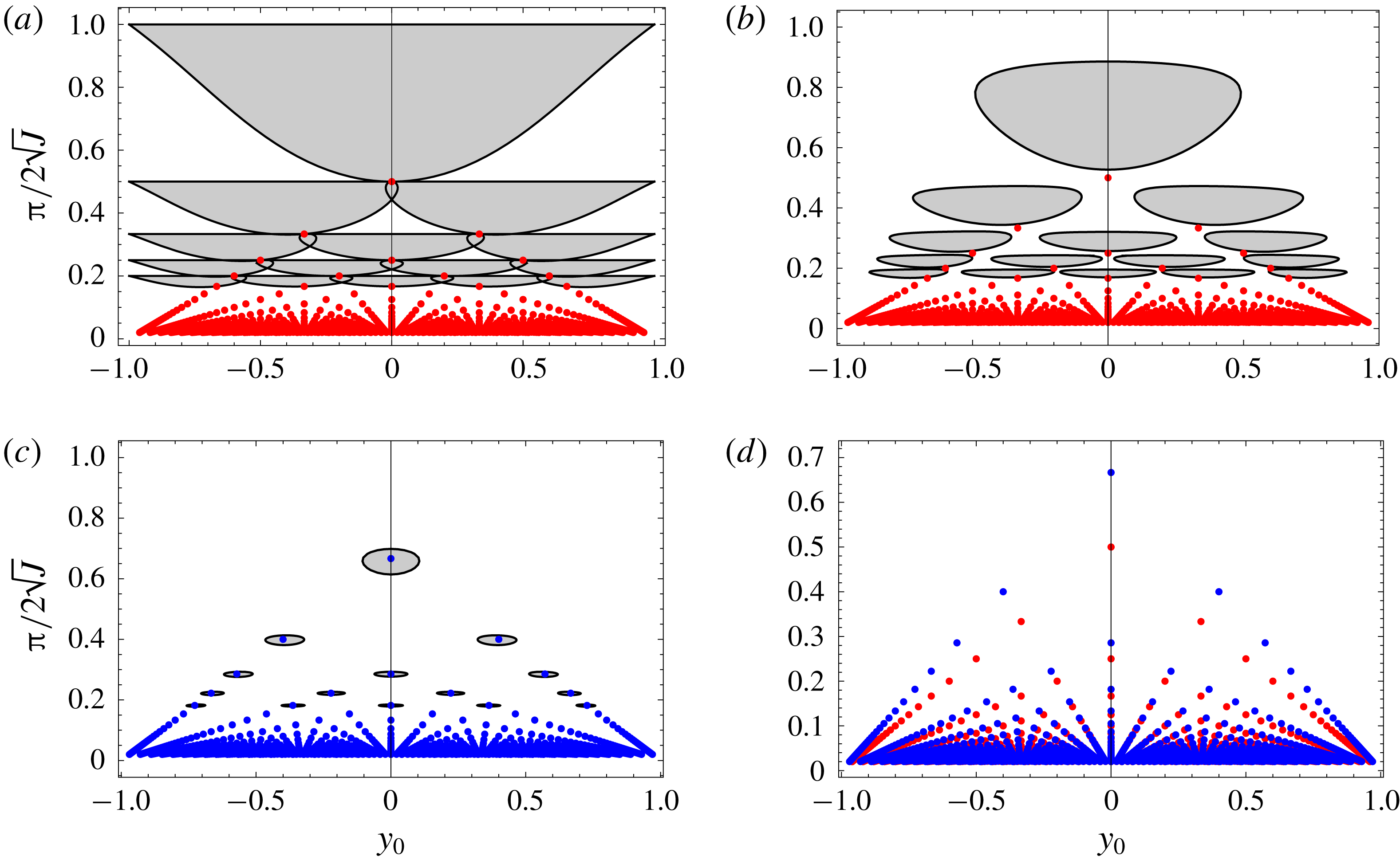
Instability diagrams for two-dimensional waves,
 $\unicode[STIX]{x1D719}=0$
, and
 $k=0$
. Shaded regions are unstable. Red dots are where neutral curves cross according to (3.4c
) and (3.10b
) at
 $Ri_{0}=0$
. Blue dots are neutral points given by (3.17) when
 $Ri_{0}=1/4$
. (a) Neutral curves for
 $Ri_{0}=0$
; (b) neutral curves for
 $Ri_{0}=0.1$
; (c) neutral curves for
 $Ri_{0}=0.24$
; (d) illustration of the relationship between the red dots, defined for
 $Ri_{0}=0$
, and the blue dots, defined for
 $Ri_{0}=1/4$
.

This truncation of the instability regime for non-zero
 $Ri_{0}$
is essentially the same as that found by Howard & Maslowe (Reference Howard and Maslowe1973). In both cases there is a fixed ratio between the constant term and the quadratic coefficient in
 $N^{2}$
. In Howard and Maslowe this ratio is
 $1/a^{2}$
and the magnitude of these terms is controlled by a bulk Richardson number. In our problem this ratio is
 $Ri_{0}/J$
, and the magnitude is controlled by
 $\sec ^{2}\unicode[STIX]{x1D719}$
, see (2.8).
However, this stabilization for
 $Ri_{0}\neq 0$
need not occur if
 $Ri_{0}$
and
 $J$
can be varied independently, such that
 $Ri_{0}<1/4$
. This is possible if we fix
 $\unicode[STIX]{x1D719}$
and vary
 $J$
. The fractal behaviour of figures 4 and 5 occurs as
 $\unicode[STIX]{x1D719}\rightarrow \unicode[STIX]{x03C0}/2$
for any fixed
 $J$
, and the same limit is reached when
 $J\rightarrow \infty$
for any fixed
 $\unicode[STIX]{x1D719}$
. Figure 7 shows the corresponding fractal behaviour for two-dimensional waves for several values of
 $Ri_{0}$
. The choice for the vertical axis was made so that the horizontal neutral curves given by (3.4c
) for
 $\unicode[STIX]{x1D719}=k=0$
are at
 $1/n$
for
 $n=1,2,3,\ldots$
. Note that when, as here, the coordinate chosen for the vertical axis is proportional to
 $J^{-1/2}$
, the red dots given by (3.10b
) lie exactly on straight lines for all
 $J$
; this is not just a limiting behaviour, as occurs in figure 5 when
 $\unicode[STIX]{x1D719}\rightarrow \unicode[STIX]{x03C0}/2$
.
In addition to the fractal behaviour of the red dots in figures 4, 5 and 7, given by (3.10b
) for
 $Ri_{0}=0$
, there is another fractal of points, shown in figure 7 by blue dots, that can be calculated explicitly when
 $Ri_{0}=1/4$
.
When
 $c=y_{0}$
, and
 $\unicode[STIX]{x1D719}=0$
(for simplicity), equation (2.8) reduces to
 $$\begin{eqnarray}\displaystyle v^{\prime \prime }+\left[\frac{Ri_{0}}{(y-y_{0})^{2}}+J-k^{2}\right]v=0, & & \displaystyle\end{eqnarray}$$
with general solution
 $$\begin{eqnarray}\displaystyle & \displaystyle v=A\sqrt{y-y_{0}}\text{J}_{\unicode[STIX]{x1D708}}(\sqrt{J-k^{2}}[y-y_{0}])+B\sqrt{y-y_{0}}\text{Y}_{\unicode[STIX]{x1D708}}(\sqrt{J-k^{2}}[y-y_{0}]), & \displaystyle\end{eqnarray}$$
 $$\begin{eqnarray}\displaystyle & \displaystyle \unicode[STIX]{x1D708}=\sqrt{1/4-Ri_{0}}, & \displaystyle\end{eqnarray}$$
 $\text{J}_{\unicode[STIX]{x1D708}}$
and
 $\text{Y}_{\unicode[STIX]{x1D708}}$
are Bessel functions of order
 $\unicode[STIX]{x1D708}$
, and
 $A$
and
 $B$
are arbitrary constants. Applying the homogeneous boundary conditions,
 $v(\pm 1)=0$
, to (3.14), and choosing
 $y_{0}=0$
, allows Howard & Maslowe’s results to be reproduced, i.e. the solid neutral curves in figure 1, (but not the dashed neutral curves).
Further simplification is possible in the case
 $Ri_{0}=1/4$
. Instability is not possible at this value, but neutral waves with
 $c=y_{0}$
still exist for particular combinations of
 $y_{0}$
and
 $J$
. Neutral waves at
 $Ri_{0}=1/4$
can be constructed using just the
 $\text{J}_{0}$
solution, i.e. setting
 $B=0$
in (3.14). It can be shown using properties of the zeros of the
 $\text{J}_{0}$
and
 $\text{Y}_{0}$
Bessel functions that real solutions are only possible when
 $B=0$
because
 $\text{Y}_{0}$
is complex for negative arguments. Applying the homogeneous boundary conditions to (3.14) with
 $B=0$
and
 $Ri_{0}=1/4$
gives
 $$\begin{eqnarray}\displaystyle 0=\text{J}_{0}(\sqrt{J-k^{2}}[1-y_{0}]),\quad 0=\text{J}_{0}(-\sqrt{J-k^{2}}[1+y_{0}]). & & \displaystyle\end{eqnarray}$$
Let
 $Z_{n}$
be the
 $n$
th zero of
 $\text{J}_{0}$
, i.e.
 $\text{J}_{0}(Z_{n})=0$
, where
 $0<Z_{1}<Z_{2}<Z_{3}<\ldots \,$
. Solutions to (3.15) can then be obtained from
 $$\begin{eqnarray}\displaystyle \sqrt{J-k^{2}}(1-y_{0})=Z_{n},\quad \sqrt{J-k^{2}}(1+y_{0})=Z_{m}, & & \displaystyle\end{eqnarray}$$
giving
 $$\begin{eqnarray}\displaystyle J=\frac{1}{4}(Z_{n}+Z_{m})^{2}+k^{2},\quad y_{0}=\frac{Z_{m}-Z_{n}}{Z_{n}+Z_{m}}. & & \displaystyle\end{eqnarray}$$
The case
 $m=n$
gives
 $y_{0}=0$
and
 $J=Z_{n}^{2}+k^{2}$
, and the blue dots in figure 1(a) are given by
 $n=1$
and
 $n=2$
(
 $Z_{1}=2.405$
,
 $Z_{2}=5.520$
), and the blue dot in figure 1(b) is given by
 $n=1$
.
In the limit
 $n\gg 1$
,
 $$\begin{eqnarray}\displaystyle Z_{n}\sim \unicode[STIX]{x03C0}\left(n-{\textstyle \frac{1}{4}}\right)+O(n^{-1}). & & \displaystyle\end{eqnarray}$$
Using the asymptotic formula (3.18) for both
 $Z_{n}$
and
 $Z_{m}$
in (3.17), and writing
 $n=n_{2}-n_{1}$
and
 $m=n_{1}$
gives
 $$\begin{eqnarray}\displaystyle J\sim \frac{\unicode[STIX]{x03C0}^{2}}{4}(n_{2}-1/2)^{2}+k^{2},\quad y_{0}\sim \frac{2n_{1}-n_{2}}{n_{2}-1/2}, & & \displaystyle\end{eqnarray}$$
which takes a very similar form to the expressions for the red dots, (3.4c
) and (3.10b
). This explains why the red dots and blue dots appear as pairs slightly shifted from one another, and shows that the blue dots lie on the same straight lines as the red dots when
 $k=0$
.
The numerical evidence in figure 7(c) suggests that at
 $Ri_{0}=0.24$
there is a small approximately elliptical neutral curve surrounding each blue dot, though this has only been verified for the top five rows of blue dots in this figure. In the following section we develop asymptotic theories to investigate the behaviour near all blue dots as
 $Ri_{0}\rightarrow 1/4$
, and near all red dots as
 $Ri_{0}\rightarrow 0$
.
4 Higher-order asymptotic theories in the fractal limit
In the previous section infinite sets of points were located in parameter space that have fractal properties, and the numerical evidence suggests that these points play an important role in organizing neutral curves in the parameter plane. The numerical results lead us to the following conjectures:
(i) When
 $Ri_{0}=0$
there are infinitely many pairs of
 $J$
and
 $y_{0}$
, given by (3.4c
) and (3.10b
), where neutral curves cross each other; these points are represented by red dots in figures 4, 5 and 7.
(ii) When
 $Ri_{0}=1/4$
there are infinitely many pairs of
 $J$
and
 $y_{0}$
, given by (3.17), and at each of these points an unstable region bounded by an approximately elliptical neutral curve appears as soon as
 $Ri_{0}$
is reduced below
 $1/4$
; these points are represented by blue dots in figure 7.
Although further numerical solutions can support these conjectures, or could disprove them, they cannot establish whether they are true. Therefore, we develop asymptotic theories valid in small neighbourhoods of the red dots, and in small neighbourhoods of the blue dots. These dots are generated by pairs of integers, and the theories are derived for arbitrary values of these integers, thus allowing us to make statements about all dots simultaneously.
In the following we consider two-dimensional waves; the generalization to three-dimensional waves only requires replacing
 $Ri_{0}$
by
 $Ri_{0}\sec ^{2}\unicode[STIX]{x1D719}$
. Some of the intermediate steps in the calculations generate many terms, and were carried out with a symbolic manipulation package.
4.1 Neutral curve crossing points
Let
 $\unicode[STIX]{x1D716}\ll 1$
be our perturbation parameter, and we expand quantities in powers of
 $\unicode[STIX]{x1D716}$
about their values given by (3.4c
) and (3.10b
) (the red dots in the figures). It turns out that the first non-neutral correction to
 $c$
appears at
 $O(\unicode[STIX]{x1D716}^{3})$
, and we can arrange for the first non-neutral effects of small
 $Ri_{0}$
to also appear at this order if we choose
 $Ri_{0}=O(\unicode[STIX]{x1D716}^{2})$
. Therefore, let
 $$\begin{eqnarray}\displaystyle J=\frac{\unicode[STIX]{x03C0}^{2}n^{2}}{4}+k^{2}+J_{1}\unicode[STIX]{x1D716},\quad y_{0}=y_{00}+y_{1}\unicode[STIX]{x1D716},\quad Ri_{0}=Ri_{00}\unicode[STIX]{x1D716}^{2}, & & \displaystyle\end{eqnarray}$$
 $$\begin{eqnarray}\displaystyle c=y_{00}+c_{1}\unicode[STIX]{x1D716}+c_{2}\unicode[STIX]{x1D716}^{2}+c_{3}\unicode[STIX]{x1D716}^{3},\quad v=v_{0}+v_{1}\unicode[STIX]{x1D716}+v_{2}\unicode[STIX]{x1D716}^{2}+v_{3}\unicode[STIX]{x1D716}^{3},\quad y_{00}=\frac{2m-n}{n}, & & \displaystyle \nonumber\\ \displaystyle & & \displaystyle\end{eqnarray}$$
where
 $n$
and
 $m$
are positive integers and
 $1\leqslant m<n$
. Substitute these expressions into (2.8), then equating coefficients of like powers of
 $\unicode[STIX]{x1D716}$
leads to a sequence of equations for
 $v_{0}$
,
 $v_{1}$
,
 $v_{2}$
and
 $v_{3}$
, which are listed in appendix A, see (A 1).
It is necessary to obtain explicit solutions for
 $v_{0}$
,
 $v_{1}$
and
 $v_{2}$
, and then
 $c_{3}$
can be obtained from applying a solvability condition to the equation for
 $v_{3}$
, (A 1d
). An outline of the main steps is given in appendix A. The neutral curves are found by setting
 $\text{Im}(c_{3})=0$
, which leads to an expression that can be written in the form
 $$\begin{eqnarray}\displaystyle 0=(b_{1}J_{1}+b_{2}y_{1})[(b_{3}J_{1}+b_{2}y_{1})J_{1}+b_{4}Ri_{00}], & & \displaystyle\end{eqnarray}$$
where the coefficients are given in (A 6). When
 $n\gg 1$
,
 $m=O(n)$
and
 $(n-m)=O(n)$
, so that
 $y_{00}=O(1)$
, and
 $y_{00}$
is not close to either
 $-1$
or
 $1$
, we can use (A 8), and when
 $k=O(1)$
, these coefficients are given at leading order by
 $$\begin{eqnarray}\displaystyle & \displaystyle b_{1}\sim 4\left\{m\ln \left(\frac{n}{m}-1\right)+n\ln m+n[\ln (2\unicode[STIX]{x03C0})+\unicode[STIX]{x1D6FE}-1]\right\}, & \displaystyle\end{eqnarray}$$
 $$\begin{eqnarray}\displaystyle & \displaystyle b_{2}\sim \unicode[STIX]{x03C0}^{2}n^{3}\ln \left(\frac{n}{m}-1\right), & \displaystyle\end{eqnarray}$$
 $$\begin{eqnarray}\displaystyle & \displaystyle b_{3}\sim b_{1}-4n, & \displaystyle\end{eqnarray}$$
 $$\begin{eqnarray}\displaystyle & \displaystyle b_{4}\sim -b_{2}\ln \left(\frac{n}{m}-1\right), & \displaystyle\end{eqnarray}$$
 $\unicode[STIX]{x03C0}$
and
 $n$
have been cancelled, and
 $\unicode[STIX]{x1D6FE}$
is Euler’s constant, see (A 7). Note that (4.3) is independent of
 $k$
. We refer to the limit
 $n\gg 1$
as the ‘fractal limit’, which is where the self-similar scaling behaviour occurs in figures 4 and 5 (as
 $\unicode[STIX]{x1D719}\rightarrow \unicode[STIX]{x03C0}/2$
) and in figure 7 (as
 $J^{-1/2}\rightarrow 0$
).
When
 $Ri_{00}=0$
, (4.2) gives three straight-line neutral curves:
 $J_{1}=0$
,
 $J_{1}=-b_{2}y_{1}/b_{1}$
and
 $J_{1}=-b_{2}y_{1}/b_{3}$
, and they all pass through
 $(y_{1},J_{1})=(0,0)$
. Therefore, when
 $Ri_{0}=0$
there is a fractal of points with
 $J$
and
 $y_{0}$
given by (3.4c
) and (3.10b
) respectively, for positive integers
 $n$
and
 $m$
,
 $1\leqslant m<n$
, where three neutral curves cross. This proves conjecture (i) above.
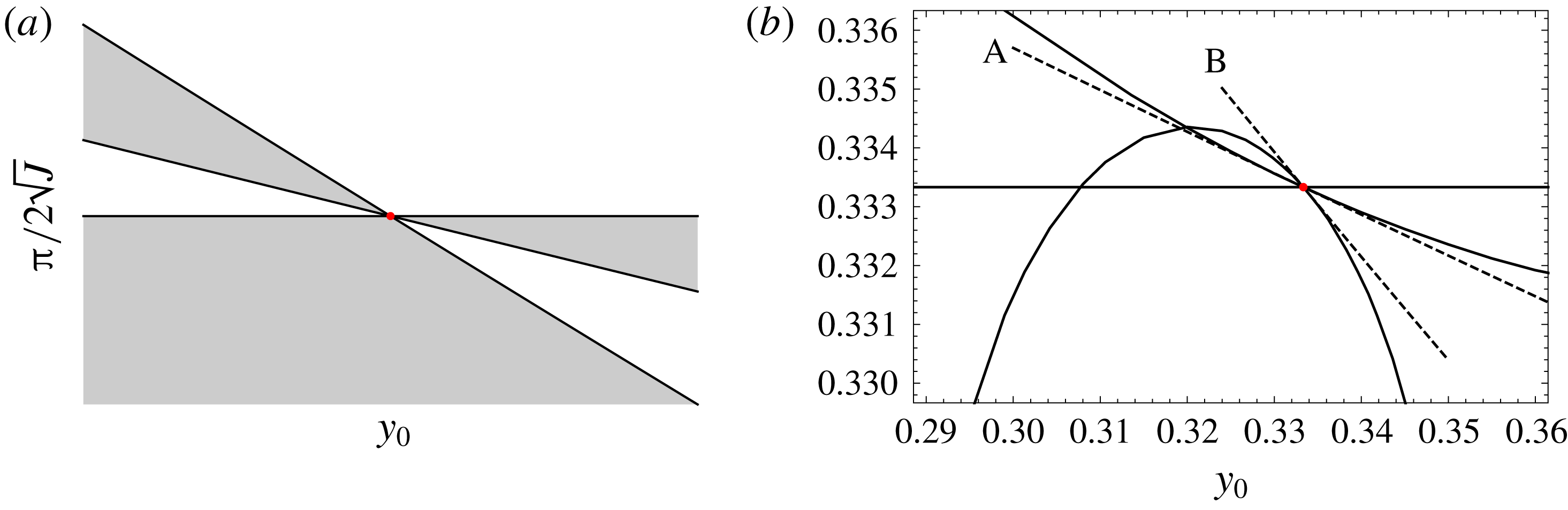
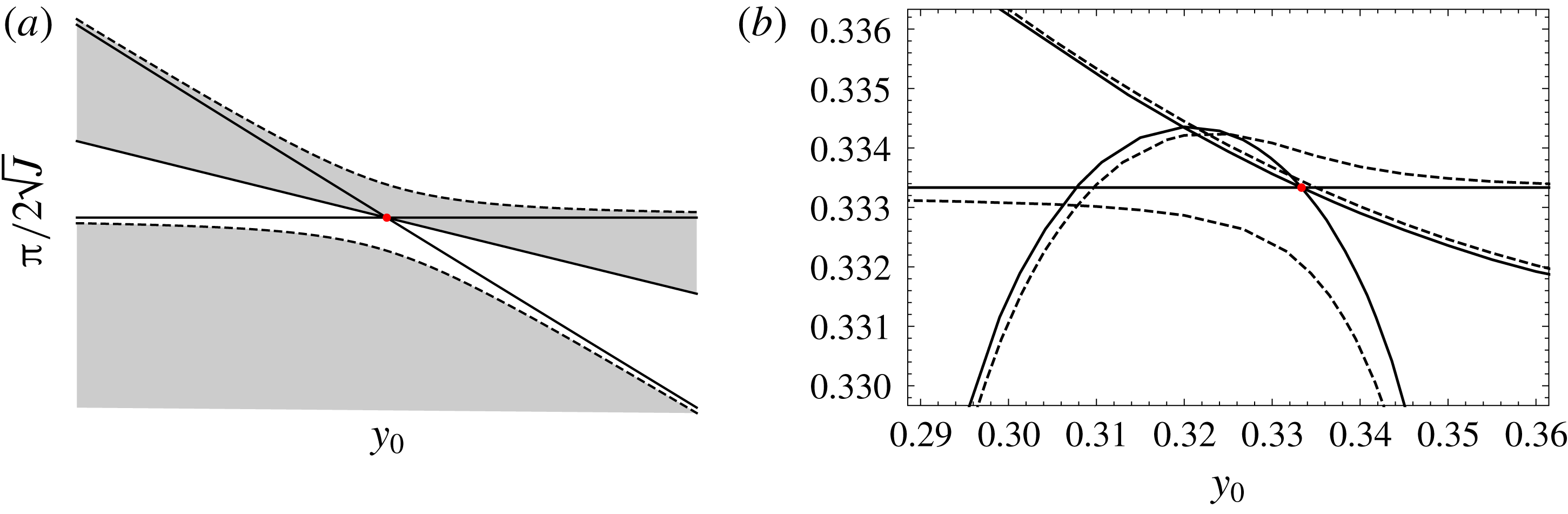
Figure 8(a) shows schematically the neutral curves, and the unstable regions, near a typical neutral curve crossing point, for
 $m>n/2$
, i.e. when
 $y_{00}>0$
. Figure 8(b) shows a quantitative comparison between the neutral curves predicted by (4.2) using the large
 $n$
approximations (4.3) for
 $n=3$
,
 $m=2$
and numerical evaluation of the full dispersion relation obtained from the exact solution (3.1). It can be seen that the asymptotics in the fractal limit can make good predictions even for small values of
 $n$
and
 $m$
.
Neutral curves near a point, marked by a red dot, where
 $J$
and
 $y_{0}$
are given by (3.4c
) and (3.10b
) respectively, for
 $Ri_{0}=Ri_{00}=0$
. (a) Schematic of neutral curves predicted by (4.2) when
 $m>n/2$
, i.e.
 $y_{00}>0$
; shaded areas are unstable. (b) Dashed line A is the neutral curve obtained from the solution
 $J_{1}=-b_{2}y_{1}/b_{1}$
of (4.2); dashed line B is the neutral curve obtained from the solution
 $J_{1}=-b_{2}y_{1}/b_{3}$
of (4.2). Both dashed lines are evaluated using (4.3) for
 $n=3$
,
 $m=2$
. Solid lines in (b) are neutral curves from numerical solutions obtained from the exact solution (3.1).

When
 $Ri_{00}>0$
the pair of neutral curves
 $J_{1}=0$
and
 $J_{1}=-b_{2}y_{1}/b_{3}$
that exist for
 $Ri_{00}=0$
reconnect as shown in figure 9(a), and no longer pass through the red dot. This pair of neutral curves at
 $Ri_{00}>0$
asymptote towards the corresponding straight line neutral curves that exist for
 $Ri_{00}=0$
as distance from the red dot increases. The neutral curve
 $J_{1}=-b_{2}y_{1}/b_{1}$
is independent of
 $Ri_{00}$
at the order of approximation used in (4.1). Qualitatively similar behaviour is seen in the numerical solutions in figure 9(b): one neutral curve is almost independent of
 $Ri_{0}$
and remains close to the red dot; the other two neutral curves move much further away from the red dot, and asymptote towards the
 $Ri_{0}=0$
results far from the red dot.
Neutral curves near a point, marked by a red dot, where
 $J$
and
 $y_{0}$
are given by (3.4c
) and (3.10b
) respectively. Solid lines are neutral curves for
 $Ri_{0}=Ri_{00}=0$
: (a) dashed lines are neutral curves shown schematically for (4.2) and
 $Ri_{00}>0$
, when
 $m>n/2$
, i.e.
 $y_{00}>0$
. Shaded regions are unstable. (b) Neutral curves obtained from numerical solutions of the exact dispersion relation obtained from (3.1). Dashed lines in (b) are neutral curves for
 $Ri_{0}=0.001$
and red dot is for
 $n=3$
,
 $m=2$
.

However, there is a second mode that is unstable near each red dot. The stable and unstable regions indicated in figures 8(a) and 9(a) refer only to the mode with the sinusoidal eigenfunction given in (3.4). When the second mode is included in the analysis, some regions that are stable in figures 8(a) and 9(a) are found to be unstable.
In the following subsection we show that there is a branch point, where the second unstable mode joins the sinusoidal mode, close to every neutral curve crossing point. Each branch point becomes asymptotically close to its associated neutral curve crossing point in the fractal limit. There is thus also a fractal of branch points in the parameter plane.
4.2 Branch points near neutral curve crossing points
There is a case where branch points can be obtained exactly. Consider a neutral curve crossing point at
 $y_{0}=y_{00}=0$
, which occurs when
 $n$
is even and
 $m=n/2$
, see (4.1f
). In this case the coefficient of
 $c_{1}$
in the solvability condition (3.8) is zero (the integrand of the integral is an odd function when
 $y_{0}=0$
and
 $n$
is an even integer). This solvability condition cannot then be satisfied, showing that the perturbation expansion (3.5) is inappropriate in this case. Huppert (Reference Huppert1973) treated this case by analysing the asymptotic form of the exact Whittaker function solutions (3.1). Alternatively, the perturbation expansion (3.5) can be rectified by including
 $O(\unicode[STIX]{x1D716}^{1/2})$
terms in (3.5b
) and (3.5c
), as discussed by Banks & Drazin (Reference Banks and Drazin1973). By either method, the result is that locally the dispersion relation supports two modes, and the two modes coalesce at a branch point when
 $y_{0}=0$
and
 $n$
in (3.7) is an even integer.
In this subsection we consider neutral curve crossing points where
 $y_{00}\neq 0$
. In these cases the integral in the solvability condition (3.8) is non-zero, and so there is not a branch point at the neutral curve crossing point itself. However, when
 $n\gg 1$
, there are branch points close to each neutral curve crossing point. The perturbation expansions are found to involve inverse powers of
 $\ln n$
.
The required form of the expansions will be developed in several stages. We consider the case
 $Ri_{0}=0$
; small
 $Ri_{0}$
could be included but does not affect results qualitatively. Rather than taking a perturbation approach to the governing equation, (2.8), we consider asymptotic forms of the exact solution, (3.1). This is because Whittaker’s equation appears at leading order in the problem, and the approximations are based on large-argument asymptotics of Whittaker functions.
Let
 $$\begin{eqnarray}\displaystyle J=\frac{\unicode[STIX]{x03C0}^{2}n^{2}}{4}+k^{2}+J_{1}n,\quad y_{0}=y_{00}+\frac{y_{1}}{n},\quad c=y_{00}+\frac{c_{1}}{n},\quad y_{00}=\frac{2m-n}{n},\quad m=m_{0}n, & & \displaystyle \nonumber\\ \displaystyle & & \displaystyle\end{eqnarray}$$
where these
 $J_{1}$
,
 $y_{1}$
and
 $c_{1}$
are different from those in § 4.1. Substitute
 $Ri_{0}=\unicode[STIX]{x1D719}=0$
and (4.4) into (3.1) and (3.2), then at leading order when
 $n\gg 1$
, this solution becomes
 $$\begin{eqnarray}\displaystyle v\sim AM_{\unicode[STIX]{x1D705}_{0},\unicode[STIX]{x1D707}_{0}}(Y)+BW_{\unicode[STIX]{x1D705}_{0},\unicode[STIX]{x1D707}_{0}}(Y), & & \displaystyle\end{eqnarray}$$
where
 $$\begin{eqnarray}\displaystyle \unicode[STIX]{x1D705}_{0}=\frac{\text{i}\unicode[STIX]{x03C0}}{2}(y_{1}-c_{1}),\quad \unicode[STIX]{x1D707}_{0}=\frac{1}{2}[1-\unicode[STIX]{x03C0}^{2}(y_{1}-c_{1})^{2}]^{1/2}, & & \displaystyle\end{eqnarray}$$
 $$\begin{eqnarray}\displaystyle Y=\text{i}\unicode[STIX]{x03C0}(y+1-2m_{0})n+\frac{\text{i}}{\unicode[STIX]{x03C0}}[2J_{1}(y+1-2m_{0})-\unicode[STIX]{x03C0}^{2}c_{1}]. & & \displaystyle\end{eqnarray}$$
Applying homogeneous boundary conditions
 $v=0$
at
 $y=\pm 1$
to (4.5) leads to an approximate dispersion relation
 $$\begin{eqnarray}\displaystyle 0=M_{\unicode[STIX]{x1D705}_{0},\unicode[STIX]{x1D707}_{0}}(Y_{+})W_{\unicode[STIX]{x1D705}_{0},\unicode[STIX]{x1D707}_{0}}(Y_{-})-M_{\unicode[STIX]{x1D705}_{0},\unicode[STIX]{x1D707}_{0}}(Y_{-})W_{\unicode[STIX]{x1D705}_{0},\unicode[STIX]{x1D707}_{0}}(Y_{+}), & & \displaystyle\end{eqnarray}$$
where
 $Y_{+}$
is
 $Y$
evaluated at
 $y=1$
, and
 $Y_{-}$
is
 $Y$
evaluated at
 $y=-1$
,
 $$\begin{eqnarray}\displaystyle Y_{+}=2\text{i}\unicode[STIX]{x03C0}(n-m)+\frac{\text{i}}{\unicode[STIX]{x03C0}}[4J_{1}(1-m_{0})-\unicode[STIX]{x03C0}^{2}c_{1}],\quad Y_{-}=-2\text{i}\unicode[STIX]{x03C0}m-\frac{\text{i}}{\unicode[STIX]{x03C0}}[4J_{1}m_{0}+\unicode[STIX]{x03C0}^{2}c_{1}]. & & \displaystyle \nonumber\\ \displaystyle & & \displaystyle\end{eqnarray}$$
Note that
 $Y_{+},Y_{-}=O(n)$
, allowing the following large-argument asymptotic approximations to be used for the Whittaker functions
 $$\begin{eqnarray}\displaystyle & \displaystyle M_{\unicode[STIX]{x1D705}_{0},\unicode[STIX]{x1D707}_{0}}(Y_{\pm })\sim \unicode[STIX]{x1D6E4}(1+2\unicode[STIX]{x1D707}_{0})\left[\frac{\text{e}^{Y_{\pm }/2-\unicode[STIX]{x1D705}_{0}\ln Y_{\pm }}}{\unicode[STIX]{x1D6E4}(\unicode[STIX]{x1D707}_{0}-\unicode[STIX]{x1D705}_{0}+1/2)}+\frac{\text{e}^{-Y_{\pm }/2+\unicode[STIX]{x1D705}_{0}\ln Y_{\pm }\pm \text{i}\unicode[STIX]{x03C0}(\unicode[STIX]{x1D707}_{0}-\unicode[STIX]{x1D705}_{0}+1/2)}}{\unicode[STIX]{x1D6E4}(\unicode[STIX]{x1D707}_{0}+\unicode[STIX]{x1D705}_{0}+1/2)}\right] & \displaystyle\end{eqnarray}$$
 $$\begin{eqnarray}\displaystyle & \displaystyle W_{\unicode[STIX]{x1D705}_{0},\unicode[STIX]{x1D707}_{0}}(Y_{\pm })\sim \text{e}^{-Y_{\pm }/2+\unicode[STIX]{x1D705}_{0}\ln Y_{\pm }}, & \displaystyle\end{eqnarray}$$
 $\unicode[STIX]{x1D6E4}(x)$
is the gamma function. Substituting (4.9) into (4.7) gives
 $$\begin{eqnarray}\displaystyle 0 & = & \displaystyle \unicode[STIX]{x1D6E4}(\unicode[STIX]{x1D707}_{0}-\unicode[STIX]{x1D705}_{0}+1/2)[\text{e}^{\text{i}\unicode[STIX]{x03C0}(\unicode[STIX]{x1D707}_{0}-\unicode[STIX]{x1D705}_{0}+1/2)}-\text{e}^{-\text{i}\unicode[STIX]{x03C0}(\unicode[STIX]{x1D707}_{0}-\unicode[STIX]{x1D705}_{0}+1/2)}]\nonumber\\ \displaystyle & & \displaystyle +\,\unicode[STIX]{x1D6E4}(\unicode[STIX]{x1D707}_{0}+\unicode[STIX]{x1D705}_{0}+1/2)[\text{e}^{Y_{+}-2\unicode[STIX]{x1D705}_{0}\ln Y_{+}}-\text{e}^{Y_{-}-2\unicode[STIX]{x1D705}_{0}\ln Y_{-}}].\end{eqnarray}$$
Note from (4.8) that
 $\text{e}^{Y_{+}}$
and
 $\text{e}^{Y_{-}}$
are both
 $O(1)$
because
 $n$
and
 $m$
are real, but
 $\ln Y_{+}$
and
 $\ln Y_{-}$
are
 $O(\ln n)$
. Therefore, (4.10) can be solved using expansions in inverse powers of
 $\ln n$
. Let
 $$\begin{eqnarray}\displaystyle c_{1}=y_{1}+c_{10}/\ln n,\quad J_{1}=J_{10}/\ln n, & & \displaystyle\end{eqnarray}$$
substitute (4.6a,b
), (4.8) and (4.11) into (4.10), expand for
 $n\gg 1$
, neglect
 $O(1/n)$
terms and equate coefficients of like powers of
 $\ln n$
to give the dispersion relation
 $$\begin{eqnarray}\displaystyle \unicode[STIX]{x1D6E5}=\text{i}\unicode[STIX]{x03C0}^{3}[1-\text{e}^{\text{i}\unicode[STIX]{x03C0}(y_{1}-c_{10})}]c_{10}+\unicode[STIX]{x03C0}^{2}c_{10}\ln \left(\frac{1}{m_{0}}-1\right)+4J_{10}=0. & & \displaystyle\end{eqnarray}$$
The conditions for a branch point, where two solutions for
 $c_{10}$
coincide, are
 $$\begin{eqnarray}\displaystyle \unicode[STIX]{x1D6E5}=0,\quad \frac{\unicode[STIX]{x2202}\unicode[STIX]{x0394}}{\unicode[STIX]{x2202}c_{10}}=0, & & \displaystyle\end{eqnarray}$$
and substituting (4.12) into (4.13b ) gives
 $$\begin{eqnarray}\displaystyle 0=\text{i}\unicode[STIX]{x03C0}[1-\text{e}^{\text{i}\unicode[STIX]{x03C0}(y_{1}-c_{10})}]-\unicode[STIX]{x03C0}^{2}c_{10}\text{e}^{\text{i}\unicode[STIX]{x03C0}(y_{1}-c_{10})}+\ln \left(\frac{1}{m_{0}}-1\right). & & \displaystyle\end{eqnarray}$$
There is one branch point solution to (4.12) and (4.14) that gives a real
 $c_{10}$
, found by setting
 $c_{10}=y_{1}$
, which gives
 $$\begin{eqnarray}\displaystyle c_{10}=y_{1}=\frac{1}{\unicode[STIX]{x03C0}^{2}}\ln \left(\frac{1}{m_{0}}-1\right),\quad J_{10}=-\frac{1}{4}\ln ^{2}\left(\frac{1}{m_{0}}-1\right). & & \displaystyle\end{eqnarray}$$
There is also a second branch point, which can be found by solving (4.12) and (4.14) for
 $J_{10}$
and
 $y_{1}$
,
 $$\begin{eqnarray}\displaystyle J_{10}=-\frac{\unicode[STIX]{x03C0}^{3}c_{10}^{2}[\unicode[STIX]{x03C0}-\text{i}\ln (1/m_{0}-1)]}{4(1-\text{i}\unicode[STIX]{x03C0}c_{10})},\quad y_{1}=c_{10}-\frac{\text{i}}{\unicode[STIX]{x03C0}}\ln \left[\frac{\unicode[STIX]{x03C0}-\text{i}\ln (1/m_{0}-1)}{\unicode[STIX]{x03C0}(1-\text{i}\unicode[STIX]{x03C0}c_{10})}\right],\qquad \quad & & \displaystyle\end{eqnarray}$$
and searching for complex
 $c_{10}$
such that
 $\text{Im}(J_{10})=0$
and
 $\text{Im}(y_{1})=0$
in (4.16). There is no explicit solution for
 $c_{10}$
in this case for general
 $m_{0}$
, but a series solution for
 $c_{10}$
can be found in powers of
 $\ln (1/m_{0}-1)$
when
 $m_{0}\rightarrow 1/2$
,
 $$\begin{eqnarray}\displaystyle J_{10}\sim \frac{1}{64\unicode[STIX]{x03C0}^{2}}\unicode[STIX]{x1D716}^{4}+\frac{1}{128\unicode[STIX]{x03C0}^{4}}\unicode[STIX]{x1D716}^{6},\quad y_{1}\sim -\frac{1}{\unicode[STIX]{x03C0}^{2}}\unicode[STIX]{x1D716}+\frac{1}{12\unicode[STIX]{x03C0}^{4}}\unicode[STIX]{x1D716}^{3}, & & \displaystyle\end{eqnarray}$$
 $$\begin{eqnarray}\displaystyle c_{10}\sim \frac{\text{i}}{4\unicode[STIX]{x03C0}^{3}}\unicode[STIX]{x1D716}^{2}-\frac{1}{8\unicode[STIX]{x03C0}^{4}}\unicode[STIX]{x1D716}^{3},\quad \unicode[STIX]{x1D716}=\ln \left(\frac{1}{m_{0}}-1\right). & & \displaystyle\end{eqnarray}$$
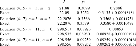
The asymptotic theories for the branch points derived in this subsection are compared to branch points obtained from numerical evaluation of the exact solution (3.1) in table 1. It can be seen that the results for (4.17) are very accurate even when
 $n=3$
, while (4.15) makes good quantitative predictions when
 $n=11$
.
Branch points where two solutions for
 $c$
coalesce, evaluated for
 $\unicode[STIX]{x1D719}=Ri_{0}=k=0$
. The ‘Exact’ results were obtained using (3.1). The asymptotic results labelled (4.15) were obtained from (4.4), (4.11) and (4.15); the asymptotic results labelled (4.17) were obtained from (4.4), (4.11) and (4.17).

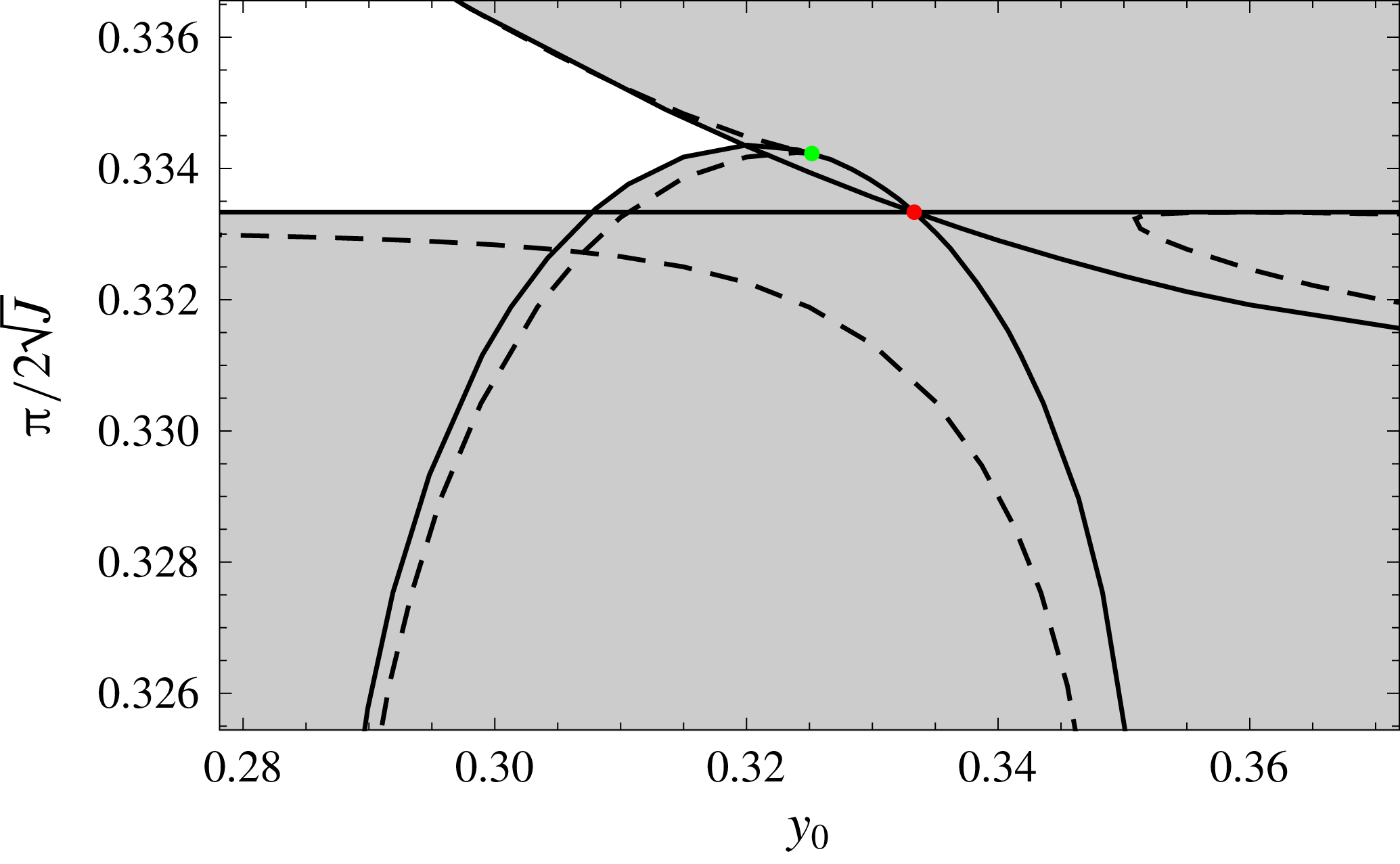
Now that the branch points close to each neutral curve crossing point have been located, we can complete the stability diagrams presented in § 4.1. Figure 10 shows the instability regions in a neighbourhood of the neutral curve crossing point (4.4d
) with
 $n=3$
and
 $m=2$
. The stable and unstable regions radiating out from the neutral curve crossing point in figure 8(a) are associated with the mode with the sinusoidal eigenfunction (3.7), but the mode that coalesces with this one to produce the branch point is unstable in a region completely surrounding the neutral curve crossing point. The only remaining stable region lies beyond the branch point, and (4.15) shows that this branch point moves away from the neutral curve crossing point as
 $m_{0}\rightarrow 0$
and as
 $m_{0}\rightarrow 1$
.
Instability diagram for
 $\unicode[STIX]{x1D719}=Ri_{0}=k=0$
near the neutral curve crossing point (4.4d
) with
 $n=3$
,
 $m=2$
marked by a red dot. Solid lines are neutral curves, shaded regions are unstable. This figure is a zoom of figure 7(a). Dashed lines are contours where
 $\text{Im}(c)=0.0001818$
. Two of these contours form a cusp at the branch point at
 $J=22.09$
,
 $y_{0}=0.3252$
, marked by the green dot, and appearing in table 1.

4.3 Neutral curves near the onset of instability
The flow (2.8) is stable when
 $Ri_{0}\geqslant 1/4$
and
 $J>0$
. In this subsection we show that when
 $Ri_{0}$
is reduced below
 $1/4$
by an arbitrarily small amount, all the blue dots shown in figure 7, which are generated by (3.17), become unstable simultaneously, and we obtain an expression for the neutral curve surrounding each blue dot.
Let
 $$\begin{eqnarray}\displaystyle Ri_{0}=\frac{1}{4}-Ri_{00}\unicode[STIX]{x1D716}^{2},\quad J=J_{00}+k^{2}+J_{1}\unicode[STIX]{x1D716},\quad y_{0}=y_{00}+y_{1}\unicode[STIX]{x1D716}, & & \displaystyle\end{eqnarray}$$
 $$\begin{eqnarray}\displaystyle c=y_{00}+c_{1}\unicode[STIX]{x1D716}+c_{2}\unicode[STIX]{x1D716}^{2},\quad v=v_{0}+v_{1}\unicode[STIX]{x1D716}+v_{2}\unicode[STIX]{x1D716}^{2}, & & \displaystyle\end{eqnarray}$$
where
 $$\begin{eqnarray}\displaystyle J_{00}=\frac{1}{4}(Z_{n}+Z_{m})^{2},\quad y_{00}=\frac{Z_{m}-Z_{n}}{Z_{n}+Z_{m}}, & & \displaystyle\end{eqnarray}$$
in accordance with (3.17), and these
 $v_{0}$
,
 $v_{1}$
,
 $v_{2}$
,
 $Ri_{00}$
,
 $J_{00}$
,
 $J_{1}$
,
 $y_{00}$
,
 $y_{1}$
,
 $c_{1}$
and
 $c_{2}$
are different from those appearing in §§ 4.1 and 4.2. As in § 3.2,
 $Z_{n}$
and
 $Z_{m}$
in (4.19) are the
 $n$
th and
 $m$
th positive zeros of the zero-order Bessel function,
 $\text{J}_{0}(Z_{n})=\text{J}_{0}(Z_{m})=0$
. Substituting (4.18) and
 $\unicode[STIX]{x1D719}=0$
into (2.8), expanding expressions for small
 $\unicode[STIX]{x1D716}$
, and equating coefficients of leading-order powers of
 $\unicode[STIX]{x1D716}$
, leads to a sequence of equations for
 $v_{0}$
,
 $v_{1}$
and
 $v_{2}$
, listed in appendix B, see (B 1). As in § 3.2, the leading-order solution is
 $$\begin{eqnarray}\displaystyle v_{0}=\sqrt{y-y_{00}}\text{J}_{0}(\sqrt{J_{00}}[y-y_{00}]), & & \displaystyle\end{eqnarray}$$
which satisfies homogeneous boundary conditions
 $v_{0}(\pm 1)=0$
when
 $J_{00}$
and
 $y_{00}$
are given by (4.19).
4.3.1 Instability at a blue dot (4.19)
Consider first each point
 $(y_{0},J)=(y_{00},J_{00}+k^{2})$
, at which
 $J_{1}=y_{1}=0$
. In this case, (B 1b
) is satisfied by
 $v_{1}=c_{1}=0$
. Substituting
 $J_{1}=y_{1}=c_{1}=0$
into (B 1c
) gives
 $$\begin{eqnarray}\displaystyle v_{2}^{\prime \prime }+\left[J_{00}+\frac{1}{4(y-y_{00})^{2}}\right]v_{2}=\frac{1}{y-y_{00}}\left[-\frac{c_{2}}{2(y-y_{00})^{2}}+\frac{Ri_{00}}{y-y_{00}}-2(J_{00}+k^{2})c_{2}\right]v_{0}. & & \displaystyle \nonumber\\ \displaystyle & & \displaystyle\end{eqnarray}$$
Equation (B 1a
) is self-adjoint, so the solvability condition for (4.21) is obtained by multiplying (4.21) by
 $v_{0}$
and integrating across the domain, taking a path below the singularities at
 $y=y_{00}$
in the complex
 $y$
plane, to give
 $$\begin{eqnarray}\displaystyle -\frac{c_{2}}{2}I_{1}+Ri_{00}I_{2}-2(J_{00}+k^{2})c_{2}I_{3}=0, & & \displaystyle\end{eqnarray}$$
where
 $$\begin{eqnarray}\displaystyle I_{1}=\int _{-1}^{1}\frac{v_{0}^{2}}{(y-y_{00})^{3}}\,\text{d}y,\quad I_{2}=\int _{-1}^{1}\frac{v_{0}^{2}}{(y-y_{00})^{2}}\,\text{d}y,\quad I_{3}=\int _{-1}^{1}\frac{v_{0}^{2}}{y-y_{00}}\,\text{d}y.\qquad & & \displaystyle\end{eqnarray}$$
Solving (4.22) for
 $c_{2}$
gives
 $$\begin{eqnarray}\displaystyle c_{2}=\frac{2Ri_{00}I_{2}}{I_{1}+4(J_{00}+k^{2})I_{3}}. & & \displaystyle\end{eqnarray}$$
It is shown in appendix B that
 $I_{1}+4(J_{00}+k^{2})I_{3}>0$
for all
 $J_{00},y_{00}$
given by (4.19), and that
 $\text{Im}(I_{2})=\unicode[STIX]{x03C0}$
. Therefore,
 $\text{Im}(c_{2})>0$
for all points (4.19), and so all of these points are unstable for any arbitrarily small
 $1/4-Ri_{0}>0$
. This proves conjecture (ii) above.
Asymptotic estimates for (4.23) can be obtained by substituting the asymptotic expansions (B 3b,d,f
), which are valid for
 $Z_{m},Z_{n}\gg 1$
, into (B 2) to give
 $$\begin{eqnarray}\displaystyle I_{1}\sim -\frac{8\sqrt{J_{00}}}{\unicode[STIX]{x03C0}},\quad I_{2}\sim -\frac{2y_{00}}{\unicode[STIX]{x03C0}(1-y_{00}^{2})\sqrt{J_{00}}}+\text{i}\unicode[STIX]{x03C0},\quad I_{3}\sim \frac{2\unicode[STIX]{x1D6FE}+6\ln 2+\ln [(1-y_{00}^{2})J_{00}]}{\unicode[STIX]{x03C0}\sqrt{J_{00}}}, & & \displaystyle \nonumber\\ \displaystyle & & \displaystyle\end{eqnarray}$$
where
 $\unicode[STIX]{x1D6FE}$
is Euler’s constant, given in (A 7). Substituting (4.25) into (4.24), and expanding for large
 $J_{00}$
, with
 $k=O(1)$
, gives
 $$\begin{eqnarray}\displaystyle c_{2}\sim \frac{\text{i}\unicode[STIX]{x03C0}^{2}Ri_{00}}{2\{2\unicode[STIX]{x1D6FE}+6\ln 2-2+\ln [J_{00}(1-y_{00}^{2})]\}\sqrt{J_{00}}} & & \displaystyle\end{eqnarray}$$
and hence, using (4.18),
 $$\begin{eqnarray}\displaystyle c\sim y_{00}+\frac{\text{i}\unicode[STIX]{x03C0}^{2}(1/4-Ri_{0})}{2\{2\unicode[STIX]{x1D6FE}+6\ln 2-2+\ln [J_{00}(1-y_{00}^{2})]\}\sqrt{J_{00}}}. & & \displaystyle\end{eqnarray}$$
It turns out that (4.27), which was derived under the assumption
 $Z_{m},Z_{n}\gg 1$
, is accurate even for the smallest
 $Z_{n}$
and
 $Z_{m}$
. For example, substituting
 $m=2$
and
 $n=1$
in (4.19) gives
 $J_{00}=15.701$
and
 $y_{00}=0.39310$
, and evaluating the exact solution (3.1) for these values and
 $Ri_{0}=0.23$
and
 $k=\unicode[STIX]{x1D719}=0$
gives
 $c=0.39303+0.00418\text{i}$
, while (4.27) gives
 $c=0.39310+0.00422\text{i}$
. Note that (4.27) is independent of
 $k$
.
Having shown that each point (4.19), i.e. every blue dot in figure 7, becomes unstable as soon as
 $Ri_{0}$
is reduced below
 $1/4$
, we now obtain an asymptotic approximation for the neutral curve that surrounds every such point.
4.3.2 Neutral curves surrounding (4.19)
The details are summarized in appendix B; we give only an outline here. Equations (B 1) are considered when
 $J_{1},y_{1},v_{1},c_{1}\neq 0$
. A solvability condition is required for (B 1b
), which determines
 $c_{1}$
, and
 $c_{1}$
is real, see (B 6). Then an explicit solution for
 $v_{1}$
is obtained in the form of (B 9), satisfying homogeneous boundary conditions, which is substituted into (B 1c
), and a solvability condition is applied to determine
 $c_{2}$
, which is complex. The neutral curve in the neighbourhood of the point (4.19) is then found by setting
 $\text{Im}(c_{2})=0$
, resulting in the equation for an ellipse centred on (4.19), which in the
 $(y_{1},J_{1})$
plane is given by
 $$\begin{eqnarray}\displaystyle d_{1}y_{1}^{2}+d_{2}J_{1}^{2}+d_{3}y_{1}J_{1}=d_{4}. & & \displaystyle\end{eqnarray}$$
In the limit
 $J_{00}\gg 1$
, the coefficients
 $d_{1}$
,
 $d_{2}$
,
 $d_{3}$
and
 $d_{4}$
, are given in (B 11). The term
 $d_{3}y_{1}J_{1}$
produces a rotation of the major and minor axes relative to the
 $y_{1}$
and
 $J_{1}$
axes, but the angle of rotation is small in this limit because
 $|d_{3}|\ll d_{1}$
. Note that
 $d_{1}$
,
 $d_{2}$
and
 $d_{4}$
are invariant when
 $n$
and
 $m$
are interchanged, and are all positive, but
 $d_{3}$
changes sign.
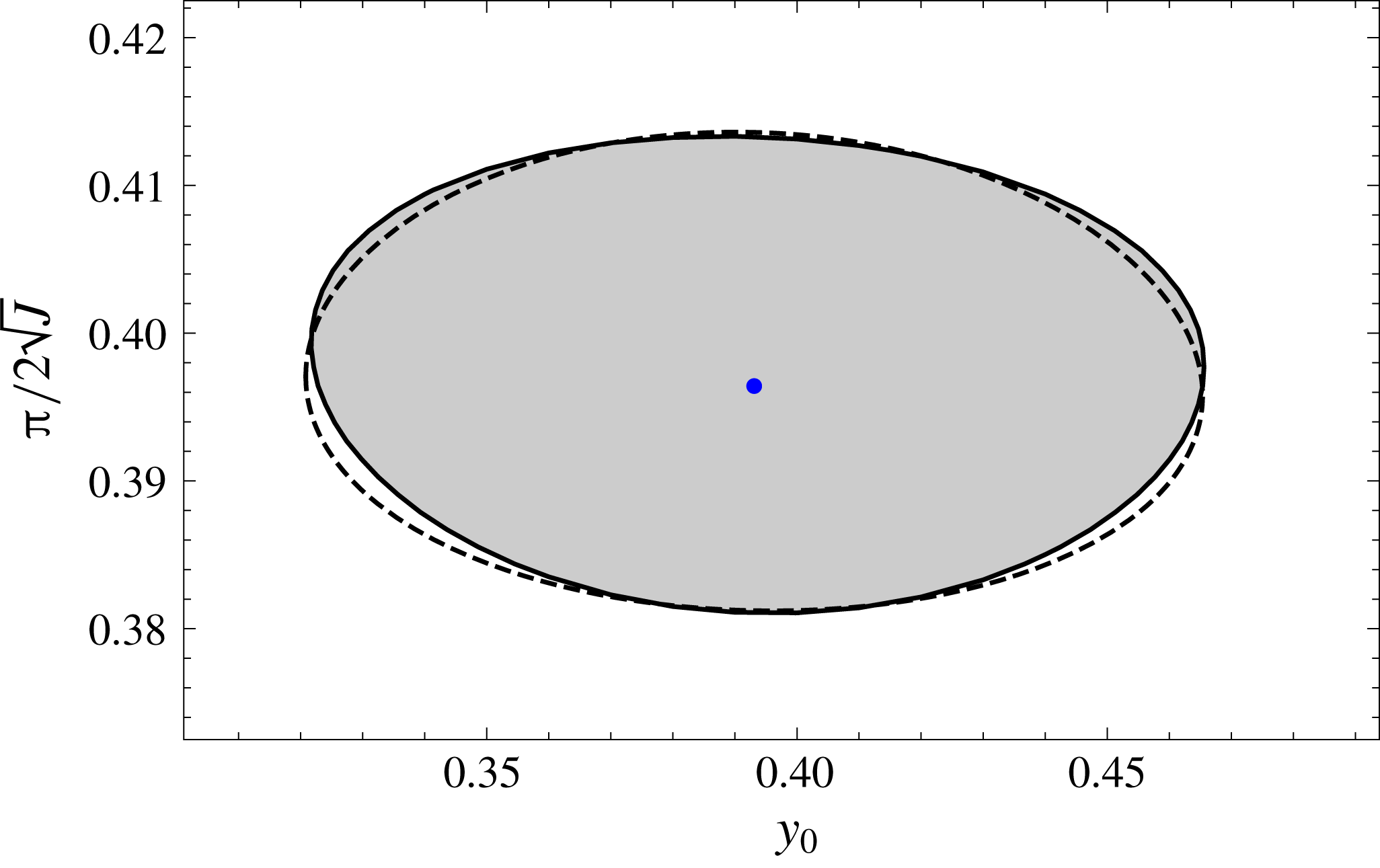
Figure 11 shows a comparison between the neutral curve from the asymptotic theory (4.28), which is based on
 $Ri_{0}\rightarrow 1/4$
and
 $J\gg 1$
, i.e.
 $n,m\gg 1$
, and a neutral curve obtained from the exact solution (3.1). There is excellent agreement even at these modest values of
 $n$
and
 $m$
.
Instability diagram for
 $\unicode[STIX]{x1D719}=k=0$
and
 $Ri_{0}=0.24$
. The blue dot marks the point
 $J=J_{00}$
and
 $y_{0}=y_{00}$
given by (4.19) for
 $m=2$
and
 $n=1$
. The solid line is the neutral curve obtained from the exact solution (3.1); shaded region is unstable; dashed line is the prediction for the neutral curve made by the asymptotic theory (4.28) using the coefficients (B 11), which were derived in the limit
 $m,n\gg 1$
, and evaluated here for
 $m=2$
and
 $n=1$
. This figure is a zoom of figure 7(c).

Note that the coefficients (B 11) take a particularly simple form when
 $m=n$
, which corresponds to an expansion about
 $y_{00}=0$
,
 $$\begin{eqnarray}\displaystyle d_{1}=\unicode[STIX]{x03C0}^{6}(4n-1)^{6},\quad d_{2}=2^{8}(4n-1)^{2}[\ln (4n-1)+\ln (2\unicode[STIX]{x03C0})+\unicode[STIX]{x1D6FE}-1]^{2}, & & \displaystyle\end{eqnarray}$$
 $$\begin{eqnarray}\displaystyle d_{3}=0,\quad d_{4}=2^{4}\unicode[STIX]{x03C0}^{4}(4n-1)^{4}[\ln (4n-1)+\ln (2\unicode[STIX]{x03C0})+\unicode[STIX]{x1D6FE}-1]^{2}Ri_{00}. & & \displaystyle\end{eqnarray}$$
In this case the major and minor axes of the ellipse are aligned with the
 $J_{1}$
and
 $y_{1}$
axes (
 $d_{3}=0$
), and the semi-axes in the
 $J_{1}$
and
 $y_{1}$
directions are
 $$\begin{eqnarray}\displaystyle J_{1}=\frac{\unicode[STIX]{x03C0}^{2}}{4}(4n-1)\sqrt{Ri_{00}},\quad y_{1}=\frac{4[\ln (4n-1)+\ln (2\unicode[STIX]{x03C0})+\unicode[STIX]{x1D6FE}-1]}{\unicode[STIX]{x03C0}(4n-1)}\sqrt{Ri_{00}},\quad & & \displaystyle\end{eqnarray}$$
respectively. It is interesting to compare the width of the ellipses given by (4.30b
) with the separation between adjacent ellipses with almost the same
 $J_{00}$
shown in figure 7(b,c). At
 $Ri_{0}=0.24$
, the ellipses shown are widely separated in
 $y_{0}$
, but at
 $Ri_{0}=0.1$
, the ellipses with larger
 $J$
almost overlap. The centres of each ellipse can be estimated for
 $n,m\gg 1$
by substituting (3.18) for
 $m$
and
 $n$
into (4.19) giving
 $$\begin{eqnarray}\displaystyle J_{00}\sim \frac{\unicode[STIX]{x03C0}^{2}}{16}[2(n+m)-1]^{2},\quad y_{00}\sim \frac{2(m-n)}{2(n+m)-1}. & & \displaystyle\end{eqnarray}$$
The centres at
 $(n,m)=(n_{0},n_{0})$
and at
 $(n,m)=(n_{0}-1,n_{0}+1)$
have almost the same
 $J_{00}$
, and the distance between them is
 $4/(4n_{0}-1)$
in
 $y_{0}$
. Therefore, the neutral curve ellipses have centres that are
 $O(1/n)$
apart in the
 $y_{0}$
direction, and (4.30b
) shows that the width of the ellipses in the
 $y_{0}$
direction is
 $O((\ln n)/n)$
.
It follows that for any fixed
 $Ri_{0}$
just below
 $1/4$
, the unstable regions overlap for large enough
 $n$
. In fact, for fixed
 $Ri_{0}$
, arbitrarily many unstable regions overlap one another as
 $n\rightarrow \infty$
.
5 Conclusions
The linear stability of plane Couette flow of an inviscid fluid between horizontal plates, whose density increases monotonically with depth, has been investigated. Diffusion of the density field has been neglected, and the Boussinesq approximation has been made, so that disturbances are described by the Taylor–Goldstein equation, (2.8a
), a second-order linear ordinary differential equation. The Brunt–Väisälä frequency term,
 $N^{2}$
, varies quadratically, see (2.8b
). There are exact solutions in Whittaker functions, and versions of this flow were studied by a number of authors, including Høiland & Riis (Reference Høiland and Riis1968), Howard & Maslowe (Reference Howard and Maslowe1973), Huppert (Reference Huppert1973), Lindzen & Barker (Reference Lindzen and Barker1985) and Baines & Mitsudera (Reference Baines and Mitsudera1994). The novelty in the present paper is the introduction of the parameter denoted
 $y_{0}$
, such that the point in the flow where the local Richardson number takes its minimum value lies at
 $y=y_{0}$
. The cited previous studies all correspond to
 $y_{0}=0$
(the mid-plane between the two plates).
Choosing
 $y_{0}\neq 0$
breaks a symmetry of the system. Plotting neutral curves as a function of
 $y_{0}$
reveals an underlying fractal structure of the neutral curves. Successive generations of the self-similar structure are encountered when either: (i) the bulk Richardson number is fixed and the wave angle
 $\unicode[STIX]{x1D719}\rightarrow \unicode[STIX]{x03C0}/2$
(
 $\unicode[STIX]{x1D719}=0$
for two-dimensional waves); or (ii) the wave angle is fixed, and the bulk Richardson number becomes large. The equivalence of these two limits is due to a version of Squire’s theorem for stratified flows, see Yih (Reference Yih1955). In case (i) the fractal appears when neutral curves are plotted in the
 $(y_{0},\unicode[STIX]{x1D719})$
plane, see figure 4; in case (ii) the fractal appears when neutral curves are plotted in the
 $(y_{0},J^{-1/2})$
plane, where
 $J$
is related to the bulk Richardson number by (2.9), see figure 7.
The local Richardson number at
 $y=y_{0}$
has been denoted
 $Ri_{0}$
. A relatively straightforward analysis is possible when
 $Ri_{0}=0$
, and also when
 $Ri_{0}=1/4$
.
In the case
 $Ri_{0}=0$
, there are neutral curves that are independent of
 $y_{0}$
, producing horizontal lines in figures 4 and 7(a). Along these lines there are rational values of
 $y_{0}$
, given by (3.10), at which a degeneracy occurs, and, at leading order, waves are neutrally stable within a neighbourhood of these points. Numerical evaluation of the exact dispersion relation near a number of these points suggests that neutral curves cross at these points, shown by red dots in figures 4 and 7. These points have fractal properties, see figure 5. A higher-order asymptotic theory presented in § 4.1 confirms that at every point (3.10) three neutral curves intersect. This theory also shows how the neutral curves pull apart when
 $0<Ri_{0}\ll 1$
.
The stability diagrams are further complicated by the existence of branch points connecting two different unstable modes. It is shown in § 4.2 that there is a pair of branch points that approach asymptotically each neutral curve crossing point as
 $J\rightarrow \infty$
, or as
 $\unicode[STIX]{x1D719}\rightarrow \unicode[STIX]{x03C0}/2$
. Expressions for the locations of these branch points involve inverse powers of
 $\ln n$
, where
 $n$
is a positive integer that labels the horizontal neutral curves in the figures.
In the case
 $Ri_{0}=1/4$
, there is a set of points, given by (3.17) in terms of zeros of the
 $\text{J}_{0}$
Bessel functions, where neutral waves exist. These points, marked by blue dots in figure 7, have the same fractal structure as the neutral curve crossing points (3.10), that exist when
 $Ri_{0}=0$
. The numerical results presented in figure 7(c) show (for a finite number of these points at least) that, a small, approximately elliptical, unstable region appears when
 $Ri_{0}$
is just below
 $1/4$
. A higher-order asymptotic theory developed in § 4.3.1 confirms that every such point is unstable when
 $0<1/4-Ri_{0}\ll 1$
, and in § 4.3.2 the equation for the neutral curves is obtained in this same limit. Consideration of the semi-axes of these elliptical neutral curves, and the distance between their centres, reveals that arbitrarily many neutral curves overlap one another for any fixed
 $Ri_{0}<1/4$
.
Essentially, the fractal of red dots in figure 7 given by (3.10) is associated with zeros of trigonometric functions, and the fractal of blue dots in the same figure is associated with zeros of Bessel functions. Similar fractals may arise in other problems when the eigenfunctions are oscillatory.
The effects of viscosity and diffusion, which are present in practical situations, have not been investigated here. It is expected that they will become important in the limits where the self-similar fractal structures exist. Nonetheless, if viscosity and diffusion are weak, then a number of generations of self-similar structures following the patterns described here might be observed. Of course, viscous effects could be destabilizing, and it is not obvious that viscosity and diffusion will necessarily obliterate the fine structures of the neutral curve fractals; they may produce alternative fractal structures instead. However, diffusion of the density field would require either a quasi-steady approximation to be made, or a treatment of the initial value problem for a time-evolving basic state, as in Smyth & Peltier (Reference Smyth and Peltier1990). For some flows, it may be reasonable to include viscosity while neglecting density diffusion, leading to a steady basic state for plane Couette flow.
Davey & Reid (Reference Davey and Reid1977) carried out stability calculations for viscous plane Couette flow with
 $N^{2}=y^{2}$
, and diffusive terms included in the disturbance equations, though the basic stratification was assumed to be steady. They obtained several neutral curves corresponding to Huppert’s (Reference Huppert1973) inviscid results, and found that instability persists down to relatively low Reynolds numbers. Davey & Reid’s calculations could be readily extended to our case of
 $N^{2}=Ri_{0}+(y-y_{0})^{2}$
, to discover the effects of viscosity and density diffusion on the fractal neutral curves.
The destabilizing effects of stable stratification, and the relationship between strong stable stratification and highly oblique waves, shows that very weak density gradients can destabilize streamwise vortices. Streamwise vortices are known to play important roles in transient growth mechanisms, and also in self-sustaining mechanisms for turbulence. It is possible that weak, stray temperature gradients in experiments on plane Couette flow could destabilize these streamwise vortices. (Similar behaviour could affect experiments on pipe flow.)
A fractal of neutral curves also represents a fractal of bifurcation points, and nonlinear solutions could be continued from these points. There are analogues between the effects of rotation and stratification on the stability of flows. Nagata (Reference Nagata1990) was able to destabilize plane Couette flow by introducing a background rotation, and then to follow nonlinear solutions from the resulting bifurcation points. These solutions persisted when the rotation was reduced to zero. It would be interesting to see if nonlinear solutions arising from the fractals of neutral curves produced here by stratification are related to Nagata’s, or if they give a new family of finite amplitude solutions.
The discovery of this intricate, interlocking, self-similar, fractal set of neutral curves prompts the question of whether similar behaviour could arise in a variety of flows, or whether it is a peculiarity of this particular flow. This issue will be explored in subsequent papers, but there are good reasons to suppose that the fractal behaviour found here should indeed appear in a wide variety of stably stratified flows, provided that they satisfy certain necessary conditions.
It seems that the key ingredients for the appearance of fractals of neutral curves are the presence of shear, and of two regions of strongly stratified fluid separated by a region of weakly stratified fluid where
 $Ri<1/4$
. The flow studied here is just a particularly simple example of this fundamental configuration. The physical mechanism for the instability in such a flow can be interpreted as the interaction between internal gravity waves (IGWs) associated with one stratified region and IGWs associated with the second stratified region. This is the physical interpretation that Baines & Mitsudera (Reference Baines and Mitsudera1994) gave for the instability of the flow studied in the present paper, but the same mechanism should operate in any flow with shear and two distinct, strongly stratified regions. In fact, this instability mechanism was first seen in § 4 of Taylor (Reference Taylor1931), where two step density jumps were placed in an infinite uniform shear. Taylor described how, as the wavenumber is varied, an IGW with real
 $c$
from one density jump coalesces with an IGW with real
 $c$
from the second density jump, to form a complex conjugate pair, and thus produce instability.
However, the step density jumps considered by Taylor each only support a pair of IGWs. The important qualitative difference in behaviour of a stably stratified region of finite extent in the vertical direction, is that it supports arbitrarily many IGWs when buoyancy forces are large. This is because the vertical wavelength then becomes small compared with the vertical size of the stratified region, allowing many IGWs with a highly oscillatory structure within the stratified region. Interactions between IGWs from each stratified region then produce many instabilities, and many neutral curves, with each interaction similar to that seen by Taylor. The final necessary ingredient for producing fractals is then the presence of a parameter that breaks the symmetry between the properties of the two stratified regions (
 $y_{0}$
in the present paper). Varying this parameter then reveals the fractal. Preliminary investigations on very different flows to those studied here, suggest that versions of the fractals seen here, do indeed arise in rather general situations.
There may be dynamical implications for the appearance of fractal neutral curves. On the one hand, the linear theory predicts either exponential growth, or exponential decay (for quasi-modes). But the rich structure of the neutral curves indicates that tiny changes to the density profile parameter
 $y_{0}$
causes a given wave to switch rapidly between stability and instability. This sensitivity resembles features of non-normal systems, where the linear operator is sensitive to small changes, especially in that non-normality is strongest for streamwise vortices, and these correspond to our fractal limit. However, our calculations are inviscid and non-normality is often associated with the viscous terms.
In reality, profiles are only known to some finite precision, and will not be completely steady, and in the presence of a fractal neutral curve the dynamics is extremely sensitive to these unknowable fine details. This suggests a loss of predictability of a wave’s fate analogous to that in chaotic dynamics.
The role of stable stratification played here could just as well be played by some other body force if it also produces a restoring force to displaced streamlines. Such a body force creates neutral modes that can interact to produce instability in the presence of shear. In addition to stratification and rotation, magnetic and electric fields can also produce restoring forces, and in some astrophysical applications all of these mechanisms could be important, with extremely weak diffusive effects, which would satisfy the assumptions made here that lead to the Taylor–Goldstein equation.
The generation of fractals by the iteration of nonlinear maps, and the appearance of fractal basin boundaries at the edge of chaos, and in forced nonlinear oscillators, may have led us to think that nonlinearity in the governing equations is an essential feature of fractal behaviour. Nonetheless, fractal behaviour has been seen in linear partial differential equations before. Billiard problems, in which a particle reflects off the internal boundaries of closed domains of certain shapes can produce chaotic trajectories, see Berry (Reference Berry1981). The wave equation in the Wentzel–Kramers–Brillouin approximation (see Hinch Reference Hinch1991) produces rays that also follow these particle paths, and their reflections at boundaries, producing fractal patterns. This behaviour can arise for internal gravity waves, and Maas & Lam (Reference Maas and Lam1995), Maas (Reference Maas2005) and Maas (Reference Maas2009) have found a number of examples producing fractal patterns. However, these fractals rely on the geometry of the boundary, and usually have constant stratification and no basic flow. The domain for our fractals is an infinite parallel strip, and the stratification varies such that there is ‘tunnelling’ between wave regions, since the disturbances are of exponential type in the region where
 $Ri<1/4$
in between the strongly stratified regions where the solutions are oscillatory.
A linear eigenvalue problem can produce a dispersion relation in which parameters, wavenumbers and the phase velocity are connected by a nonlinear relationship with infinitely many roots, and this can produce fractal behaviour without nonlinearity in the governing equations. If fractal behaviour can be produced by linear ordinary differential equations, then fractal behaviour can also be produced by iterating linear maps. One way of constructing such a map is simply to solve (2.8) using a shooting method based on a Runge–Kutta discretization scheme. Qualitatively similar behaviour should also be possible in suitably constructed simpler linear maps.
When chaos and fractal behaviour were discovered in low-order nonlinear ordinary differential equations, it offered the possibility of using low-order nonlinear models to study complex processes where it had seemed that only stochastic methods were applicable. If linear systems can generate fractals, then there may be greater potential for developing linear models for complex phenomena than had been realized, and some complex behaviour attributed to nonlinearity might have an underlying linear mechanism.
Acknowledgement
This work has benefitted from discussions with my colleague at Keele, Professor Shrira, and was partly supported by EU grant FP7 612610, which is gratefully acknowledged.
Appendix A
Substitute (4.1) and
 $\unicode[STIX]{x1D719}=0$
into (2.8), and equate coefficients of powers of
 $\unicode[STIX]{x1D716}$
to give the sequence of equations
 $$\begin{eqnarray}\displaystyle \displaystyle v_{0}^{\prime \prime }+\frac{n^{2}\unicode[STIX]{x03C0}^{2}}{4}v_{0} & = & \displaystyle 0,\end{eqnarray}$$
 $$\begin{eqnarray}\displaystyle v_{1}^{\prime \prime }+\frac{n^{2}\unicode[STIX]{x03C0}^{2}}{4}v_{1} & = & \displaystyle -\left[J_{1}-\frac{(n^{2}\unicode[STIX]{x03C0}^{2}+4k^{2})(y_{1}-c_{1})}{2(y-y_{00})}\right]v_{0},\end{eqnarray}$$
 $$\begin{eqnarray}\displaystyle \displaystyle v_{2}^{\prime \prime }+\frac{n^{2}\unicode[STIX]{x03C0}^{2}}{4}v_{2} & = & \displaystyle -\left[J_{1}-\frac{(n^{2}\unicode[STIX]{x03C0}^{2}+4k^{2})(y_{1}-c_{1})}{2(y-y_{00})}\right]v_{1}\nonumber\\ \displaystyle & & \displaystyle -\,\frac{1}{2(y-y_{00})}\left[\frac{4Ri_{00}+(n^{2}\unicode[STIX]{x03C0}^{2}+4k^{2})(y_{1}-c_{1})(y_{1}-3c_{1})}{2(y-y_{00})}\right.\nonumber\\ \displaystyle & & \displaystyle \left.+\,(n^{2}\unicode[STIX]{x03C0}^{2}+4k^{2})c_{2}-4J_{1}(y_{1}-c_{1})\right]v_{0},\end{eqnarray}$$
 $$\begin{eqnarray}\displaystyle \displaystyle v_{3}^{\prime \prime }+\frac{n^{2}\unicode[STIX]{x03C0}^{2}}{4}v_{3} & = & \displaystyle -\left[J_{1}-\frac{(n^{2}\unicode[STIX]{x03C0}^{2}+4k^{2})(y_{1}-c_{1})}{2(y-y_{00})}\right]v_{2}\nonumber\\ \displaystyle & & \displaystyle -\,\frac{1}{2(y-y_{00})}\left[\frac{4Ri_{00}+(n^{2}\unicode[STIX]{x03C0}^{2}+4k^{2})(y_{1}-c_{1})(y_{1}-3c_{1})}{2(y-y_{00})}\right.\nonumber\\ \displaystyle & & \displaystyle \left.+\,(n^{2}\unicode[STIX]{x03C0}^{2}+4k^{2})c_{2}-4J_{1}(y_{1}-c_{1})\right]v_{1}\nonumber\\ \displaystyle & & \displaystyle -\,\frac{1}{2(y-y_{00})}\left\{\frac{c_{1}[4Ri_{00}+(n^{2}\unicode[STIX]{x03C0}^{2}+4k^{2})(y_{1}-c_{1})(y_{1}-2c_{1})]}{(y-y_{00})^{2}}\right.\nonumber\\ \displaystyle & & \displaystyle +\,\frac{2J_{1}(y_{1}-c_{1})(y_{1}-3c_{1})-c_{2}(2y_{1}-3c_{1})(n^{2}\unicode[STIX]{x03C0}^{2}+k^{2})}{y-y_{00}}\nonumber\\ \displaystyle & & \displaystyle \left.+\,(n^{2}\unicode[STIX]{x03C0}^{2}+4k^{2})c_{3}+4J_{1}c_{2}\right\}v_{0}.\end{eqnarray}$$
 $v_{0}$
. Therefore, the solvability condition for an inhomogeneous equation of the form
 $$\begin{eqnarray}\displaystyle v^{\prime \prime }+\frac{n^{2}\unicode[STIX]{x03C0}^{2}}{4}v=f(y), & & \displaystyle\end{eqnarray}$$
allowing homogeneous boundary conditions to be satisfied, is
 $$\begin{eqnarray}\displaystyle \int _{-1}^{1}f(t)v_{0}(t)\,\text{d}t=0. & & \displaystyle\end{eqnarray}$$
Applying (A 3) with
 $f$
given by the right-hand side of (A 1b
) gives an equation that determines
 $c_{1}$
, similar to (3.8). Applying (A 3) with
 $f$
given by the right-hand side of (A 1c
), and of (A 1d
), give equations that determine
 $c_{2}$
and
 $c_{3}$
respectively. The equation for
 $c_{2}$
requires explicit solutions for
 $v_{0}$
and
 $v_{1}$
, and the equation for
 $c_{3}$
requires explicit solutions for
 $v_{0}$
,
 $v_{1}$
and
 $v_{2}$
. The solution to an equation of the form (A 2) satisfying
 $v(-1)=0$
can be written
 $$\begin{eqnarray}\displaystyle v=\frac{2}{n\unicode[STIX]{x03C0}}\left(v_{0}\int _{-1}^{y}f(t)\cos [n\unicode[STIX]{x03C0}(t+1)/2]\,\text{d}t-\cos [n\unicode[STIX]{x03C0}(t+1)/2]\int _{-1}^{y}f(t)v_{0}(t)\,\text{d}t\right), & & \displaystyle\end{eqnarray}$$
with
 $v_{0}$
given by (3.7). If (A 3) is satisfied then the solution (A 4) also satisfies the second homogeneous boundary condition,
 $v(1)=0$
, because
 $v_{0}(1)=0$
.
Solutions for
 $v_{1}$
and
 $v_{2}$
can be developed from expressions of the form (A 4) by taking
 $f$
to be the right-hand sides of (A 1b,c
). There is no singularity on the right-hand side of (A 1b
) at
 $y=y_{00}$
because
 $v_{0}(y_{00})=0$
by (3.7) and (4.1f
), and therefore
 $v_{1}$
is non-singular at
 $y=y_{00}$
. The right-hand side of (A 1c
) is singular at
 $y=y_{00}$
, and is
 $O((y-y_{00})^{-1})$
as
 $y\rightarrow y_{00}$
, which produces logarithmic behaviour in
 $v_{2}$
due to the first integral in (A 4). However, the solvability condition for (A 1c
) produces a real
 $c_{2}$
because multiplying the right-hand side of (A 1c
) by
 $v_{0}$
regularizes this right-hand side, and it is this product that appears in (A 3), and in the second integral of (A 4). The right-hand side of (A 1d
) is
 $O((y-y_{00})^{-2})$
as
 $y\rightarrow y_{00}$
, and these terms produce simple poles in the solvability condition, whose residues contribute complex terms to
 $c_{3}$
. In addition, there are complex terms contributed by the logarithmic terms in
 $v_{2}$
.
The solutions for
 $v_{1}$
and
 $v_{2}$
, and the solvability equation for
 $c_{3}$
, can be expressed in terms of the sine and cosine integral functions, and the terms contributing to
 $\text{Im}(c_{3})$
arise just from the cosine integral function
 $$\begin{eqnarray}\displaystyle \text{Ci}(x)=-\int _{x}^{\infty }\frac{\cos t}{t}\,\text{d}t. & & \displaystyle\end{eqnarray}$$
Neutral curves are obtained by setting
 $\text{Im}(c_{3})=0$
, which can be written in the form (4.2), where the coefficients are
 $$\begin{eqnarray}\displaystyle \displaystyle b_{1} & = & \displaystyle 4\{(n^{2}\unicode[STIX]{x03C0}^{2}+4k^{2})[(m-n)\text{Ci}(2\unicode[STIX]{x03C0}m)-m\text{Ci}(2\unicode[STIX]{x03C0}[n-m])+m\ln (n/m-1)\nonumber\\ \displaystyle & & \displaystyle \,+n\ln (2\unicode[STIX]{x03C0}m)+\unicode[STIX]{x1D6FE}n]-\unicode[STIX]{x03C0}^{2}n^{3}\},\end{eqnarray}$$
 $$\begin{eqnarray}\displaystyle \displaystyle b_{2} & = & \displaystyle -\unicode[STIX]{x03C0}^{2}n^{3}(n^{2}\unicode[STIX]{x03C0}^{2}+4k^{2})\{\text{Ci}(2\unicode[STIX]{x03C0}[n-m])-\text{Ci}(2\unicode[STIX]{x03C0}m)-\ln (n/m-1)\},\end{eqnarray}$$
 $$\begin{eqnarray}\displaystyle \displaystyle b_{3} & = & \displaystyle b_{1}-4\unicode[STIX]{x03C0}^{2}n^{3},\end{eqnarray}$$
 $$\begin{eqnarray}\displaystyle \displaystyle b_{4} & = & \displaystyle \{\text{Ci}(2\unicode[STIX]{x03C0}[n-m])-\text{Ci}(2\unicode[STIX]{x03C0}m)-\ln (n/m-1)\}b_{2},\end{eqnarray}$$
 $\unicode[STIX]{x1D6FE}$
is Euler’s constant
 $$\begin{eqnarray}\displaystyle \unicode[STIX]{x1D6FE}=\lim _{x\rightarrow 0}[\text{Ci}(x)-\ln x]\approx 0.577, & & \displaystyle\end{eqnarray}$$
which arises, for example, in the evaluation of
 $v_{1}(y_{00})$
and
 $v_{2}(y_{00})$
. Note that
 $$\begin{eqnarray}\displaystyle \text{Ci}(x)\sim -\frac{1}{x^{2}} & & \displaystyle\end{eqnarray}$$
when
 $x$
is a large, even, multiple of
 $\unicode[STIX]{x03C0}$
.
Appendix B
Substituting (4.18) and
 $\unicode[STIX]{x1D719}=0$
into (2.8), and equating coefficients of like powers of
 $\unicode[STIX]{x1D716}$
gives
 $$\begin{eqnarray}\displaystyle \displaystyle v_{0}^{\prime \prime }+\left[J_{00}+\frac{1}{4(y-y_{00})^{2}}\right]v_{0} & = & \displaystyle 0,\end{eqnarray}$$
 $$\begin{eqnarray}\displaystyle \displaystyle v_{1}^{\prime \prime }+\left[J_{00}+\frac{1}{4(y-y_{00})^{2}}\right]v_{1} & = & \displaystyle -\left[\frac{c_{1}}{2(y-y_{00})^{3}}-\frac{2(J_{00}+k^{2})(y_{1}-c_{1})}{y-y_{00}}+J_{1}\right]v_{0},\qquad\end{eqnarray}$$
 $$\begin{eqnarray}\displaystyle \displaystyle v_{2}^{\prime \prime }+\left[J_{00}+\frac{1}{4(y-y_{00})^{2}}\right]v_{2} & = & \displaystyle -\left[\frac{c_{1}}{2(y-y_{00})^{3}}-\frac{2(J_{00}+k^{2})(y_{1}-c_{1})}{y-y_{00}}+J_{1}\right]v_{1}\nonumber\\ \displaystyle & & \displaystyle +\,\frac{1}{y-y_{00}}\left[-\frac{3c_{1}^{2}}{4(y-y_{0})^{3}}-\frac{c_{2}}{2(y-y_{00})^{2}}\right.\nonumber\\ \displaystyle & & \displaystyle +\,\frac{Ri_{00}-(J_{00}+k^{2})(y_{1}-c_{1})(y_{1}-3c_{1})}{y-y_{00}}\nonumber\\ \displaystyle & & \displaystyle \left.-\,2(J_{00}+k^{2})c_{2}+2(y_{1}-c_{1})J_{1}\right]v_{0}.\end{eqnarray}$$
 $x=\sqrt{J_{00}}(y-y_{00})$
, gives
 $$\begin{eqnarray}\displaystyle I_{1}=\sqrt{J_{00}}\int _{-Z_{m}}^{Z_{n}}\frac{\text{J}_{0}^{2}(x)}{x^{2}}\,\text{d}x,\quad I_{2}=\int _{-Z_{m}}^{Z_{n}}\frac{\text{J}_{0}^{2}(x)}{x}\,\text{d}x,\quad I_{3}=\frac{1}{\sqrt{J_{00}}}\int _{-Z_{m}}^{Z_{n}}\text{J}_{0}^{2}(x)\,\text{d}x,\qquad & & \displaystyle\end{eqnarray}$$
using (4.19). These integrals can be solved in terms of hypergeometric functions, and expanded for
 $|x|\gg 1$
, giving
 $$\begin{eqnarray}\displaystyle \displaystyle \int \frac{\text{J}_{0}^{2}(x)}{x^{2}}\,\text{d}x & = & \displaystyle -\frac{\text{}_{1}F_{2}(-1/2;1,1;-x^{2})}{x}\sim \left\{\begin{array}{@{}ll@{}}\displaystyle -\frac{4}{\unicode[STIX]{x03C0}}-\frac{1}{2\unicode[STIX]{x03C0}x^{2}} & \text{for }x\gg 1\\[10.0pt] \displaystyle \frac{4}{\unicode[STIX]{x03C0}}+\frac{1}{2\unicode[STIX]{x03C0}x^{2}} & \text{for }-x\gg 1,\end{array}\right.\end{eqnarray}$$
 $$\begin{eqnarray}\displaystyle \displaystyle \int \frac{\text{J}_{0}^{2}(x)}{x}\,\text{d}x & = & \displaystyle -\frac{1}{4}x^{2}\,\text{}_{3}F_{4}(1,1,3/2;2,2,2,2;-x^{2})+\ln x\nonumber\\ \displaystyle & {\sim} & \displaystyle \left\{\begin{array}{@{}ll@{}}\displaystyle -\unicode[STIX]{x1D6FE}+\ln 2-\frac{1}{\unicode[STIX]{x03C0}x} & \text{for }x\gg 1\\ \displaystyle -\unicode[STIX]{x1D6FE}+\ln 2+\text{i}\unicode[STIX]{x03C0}+\frac{1}{\unicode[STIX]{x03C0}x} & \text{for }-x\gg 1,\end{array}\right.\end{eqnarray}$$
 $$\begin{eqnarray}\displaystyle \displaystyle \int \text{J}_{0}^{2}(x)\,\text{d}x & = & \displaystyle x\,\text{}_{2}F_{3}(1/2,1/2;1,1,3/2;-x^{2})\nonumber\\ \displaystyle & {\sim} & \displaystyle \left\{\begin{array}{@{}ll@{}}\displaystyle \frac{\ln x}{\unicode[STIX]{x03C0}}+\frac{\unicode[STIX]{x1D6FE}+\ln 8}{\unicode[STIX]{x03C0}} & \text{for }x\gg 1\\[10.0pt] \displaystyle -\frac{\ln (-x)}{\unicode[STIX]{x03C0}}-\frac{\unicode[STIX]{x1D6FE}+\ln 8}{\unicode[STIX]{x03C0}} & \text{for }-x\gg 1.\end{array}\right.\end{eqnarray}$$
There is a simple pole at
 $x=0$
in the integral for
 $I_{2}$
, see (B 2b
), and its residue gives
 $\text{Im}(I_{2})=\unicode[STIX]{x03C0}$
because
 $\text{J}_{0}(0)=1$
(this can also be seen from (B 3c
) because
 $_{3}F_{4}$
is real at the end points of the range of integration, and the imaginary part comes from the
 $\ln x$
term with a path taken below the origin in the complex
 $x$
plane).
The integral
 $I_{3}>0$
because its integrand,
 $\text{J}_{0}^{2}\geqslant 0$
, see (B 2c
). The integrand for
 $I_{1}$
is
 $\text{J}_{0}^{2}(x)/x^{2}\geqslant 0$
for all
 $x\neq 0$
, see (B 2a
). However,
 $I_{1}<0$
for any integration range that includes the singularity at
 $x=0$
, and
 $I_{1}$
becomes more negative the smaller the integration range surrounding the origin becomes. Using (B 3b
) we can place the following bounds on
 $I_{1}$
,
 $$\begin{eqnarray}\displaystyle \int _{-Z_{1}}^{Z_{1}}\frac{\text{J}_{0}^{2}(x)}{x^{2}}\,\text{d}x\leqslant \frac{I_{1}}{\sqrt{J_{00}}}<-\frac{8}{\unicode[STIX]{x03C0}}\quad \Rightarrow \quad -2.5925\leqslant \frac{I_{1}}{\sqrt{J_{00}}}<-2.5465. & & \displaystyle\end{eqnarray}$$
The corresponding bound for
 $I_{3}$
is
 $$\begin{eqnarray}\displaystyle \int _{-Z_{1}}^{Z_{1}}\text{J}_{0}^{2}(x)\,\text{d}x\leqslant \sqrt{J_{00}}I_{3}\quad \Rightarrow \quad 2.2772\leqslant \sqrt{J_{00}}I_{3}. & & \displaystyle\end{eqnarray}$$
It follows from (B 4) and (B 5) that
 $I_{1}+4(J_{00}+k^{2})I_{3}>0$
for all (4.19).
The solvability condition for (B 1b
) is obtained by multiplying (B 1b
) by
 $v_{0}$
(which is the solution of the adjoint problem) and integrating across the domain, taking a path in the complex plane below singularities, to give
 $$\begin{eqnarray}\displaystyle \frac{c_{1}}{2}I_{1}-2(J_{00}+k^{2})(y_{1}-c_{1})I_{3}+J_{1}I_{4}=0, & & \displaystyle\end{eqnarray}$$
to be solved for
 $c_{1}$
, where
 $I_{1}$
and
 $I_{3}$
are given in (B 2), and
 $$\begin{eqnarray}\displaystyle I_{4}=\int _{-1}^{1}v_{0}^{2}\,\text{d}y=\frac{1}{J_{00}}\int _{-Z_{m}}^{Z_{n}}x\text{J}_{0}^{2}(x)\,\text{d}x, & & \displaystyle\end{eqnarray}$$
where
 $x=\sqrt{J_{00}}(y-y_{00})$
, using (4.19) and (4.20). The integrals
 $I_{1}$
,
 $I_{3}$
and
 $I_{4}$
are all real, so
 $c_{1}$
is real.
Multiplying (B 1c
) by
 $v_{0}$
, integrating over the domain and taking a path below singularities in the complex plane, gives the solvability condition for
 $v_{2}$
, and can be used to determine
 $c_{2}$
. This requires an explicit solution for
 $v_{1}$
, which can be obtained in terms of integrals involving the Bessel functions
 $\text{J}_{0}$
and
 $\text{Y}_{0}$
. However,
 $\text{Y}_{0}(x)$
is complex for
 $x<0$
, and it is convenient instead to express
 $v_{1}$
in terms of double integrals involving
 $\text{J}_{0}$
only. This helps in extracting the imaginary parts of complex terms, which are needed to obtain neutral curves. The equation for
 $v_{1}$
, (B 1b
), is in the form
 $$\begin{eqnarray}\displaystyle v_{1}^{\prime \prime }+\left[J_{00}+\frac{1}{4(y-y_{00})^{2}}\right]v_{1}=f(y)v_{0}, & & \displaystyle\end{eqnarray}$$
and we choose a particular solution in the form
 $$\begin{eqnarray}\displaystyle v_{1}=v_{0}\int _{-1}^{y}\frac{1}{v_{0}^{2}(t_{1})}\int _{-1}^{t_{1}}v_{0}^{2}(t_{2})f(t_{2})\,\text{d}t_{2}\,\text{d}t_{1}. & & \displaystyle\end{eqnarray}$$
This solution is singular at
 $y=y_{00}$
, and the singularities need to be extracted from the integrals, e.g.
 $$\begin{eqnarray}\displaystyle \int _{-1}^{t_{1}}\frac{v_{0}^{2}}{(t_{2}-y_{00})^{3}}\,\text{d}t_{2}=\int _{-1}^{t_{1}}\frac{v_{0}^{2}}{(t_{2}-y_{00})^{3}}-\frac{1}{(t_{2}-y_{00})^{2}}\,\text{d}t_{2}-\frac{1}{t_{1}-y_{00}}-\frac{1}{1+y_{00}}, & & \displaystyle\end{eqnarray}$$
where the integrand on the right-hand side is regular, because
 $v_{0}^{2}(t_{2})\sim (t_{2}-y_{00})+O([t_{2}-y_{00}]^{3})$
from (4.20). A similar procedure is applied to the outer integral of (B 9), and repeated for the other two terms on the right-hand side of (B 1b
). This procedure for extracting singular parts of integrals is also applied to the integrals appearing in the solvability condition for (B 1c
).
Setting the imaginary parts to zero of all the complex terms in this solvability condition gives an equation for the neutral curve surrounding the point
 $(y_{0},J)=(y_{00},J_{00}+k^{2})$
given in (4.18). However, this equation (obtained using a symbolic manipulation package), has very many terms and it is not helpful to write it out. We present instead the result in the limit
 $J_{00}\gg 1$
, in which the imaginary parts of the integrals that generate complex terms can be obtained from a combination of residue theory and evaluation in terms of hypergeometric functions with known asymptotic behaviours (like in (B 3)). In this limit the equation for the ellipse giving each neutral curve is (4.28), with coefficients
 $$\begin{eqnarray}\displaystyle \displaystyle d_{1} & = & \displaystyle \unicode[STIX]{x03C0}^{4}[2(n+m)-1]^{6}\left[\unicode[STIX]{x03C0}^{2}+\ln ^{2}\left(\frac{4n-1}{4m-1}\right)\right],\end{eqnarray}$$
 $$\begin{eqnarray}\displaystyle \displaystyle d_{2} & = & \displaystyle 64(\{[4n-1]\ln [4m-1]+[4m-1]\ln [4n-1]+2[2(n+m)-1]\nonumber\\ \displaystyle & & \displaystyle \times \,[\ln (2\unicode[STIX]{x03C0})+\unicode[STIX]{x1D6FE}-1]\}^{2}+4\unicode[STIX]{x03C0}^{2}[n-m]^{2} ),\end{eqnarray}$$
 $$\begin{eqnarray}\displaystyle \displaystyle d_{3} & = & \displaystyle 16\unicode[STIX]{x03C0}^{2}[2(n+m)-1]^{3}\left[2\unicode[STIX]{x03C0}^{2}(m-n)+\ln \left(\frac{4n-1}{4m-1}\right)\right.\nonumber\\ \displaystyle & & \displaystyle \times \,\{2[2(n+m)-1][\ln (2\unicode[STIX]{x03C0})+\unicode[STIX]{x1D6FE}-1]\nonumber\\ \displaystyle & & \displaystyle \left.+\,(4n-1)\ln (4m-1)+(4m-1)\ln (4n-1)\}\right],\end{eqnarray}$$
 $$\begin{eqnarray}\displaystyle \displaystyle d_{4} & = & \displaystyle 4\unicode[STIX]{x03C0}^{2}[2(n+m)-1]^{4}\{\ln [(4n-1)(4m-1)]+2[\ln (2\unicode[STIX]{x03C0})+\unicode[STIX]{x1D6FE}-1]\}^{2}Ri_{00},\nonumber\\ \displaystyle & & \displaystyle\end{eqnarray}$$
 $n$
and
 $m$
correspond to the subscripts of
 $Z_{n}$
and
 $Z_{m}$
in (4.19), and the approximation (3.18) has been used for both
 $n$
and
 $m$
.