





1. Introduction
Thermal convection emerges across diverse geometrical environments in both natural and industrial systems. For convection in barely confined domains, such as atmospheres (Atkinson & Wu Zhang Reference Atkinson and Wu Zhang1996), oceans (Marshall & Schott Reference Marshall and Schott1999), lakes (Bouffard & Wüest Reference Bouffard and Wüest2019), planetary mantles (Schubert Reference Schubert1992) and outer cores (Cheng et al. Reference Cheng, Stellmach, Ribeiro, Grannan, King and Aurnou2015), the lateral constraints are insignificant, regulating their large-scale structures only. However, in most cases, fluids are in contact with no-slip solid matrices enclosing fluid domains laterally. An example of extremely confined convection can be found in porous media (Hewitt, Neufeld & Lister Reference Hewitt, Neufeld and Lister2012; De Paoli Reference De Paoli2023). Since the fluids percolate through pores of solid matrices, the inertial effect is irrelevant and the Darcy law is applicable, simplifying the systems significantly. Between these extremes, we often encounter systems that are compressed only in one lateral direction, namely vertical slots, e.g. geological fractures/faults (Patterson et al. Reference Patterson, Driesner, Matthai and Tomlinson2018), hydrothermal vents (Cherkaoui & Wilcock Reference Cherkaoui and Wilcock2001), ice crevasses (Benn et al. Reference Benn, Gulley, Luckman, Adamek and Glowacki2009), magma ascent in fissures/dykes (Jones & Llewellin Reference Jones and Llewellin2021), and small engineering devices like heat exchangers (Vera & Linan Reference Vera and Linan2010) and microfluidics (Stone, Stroock & Ajdari Reference Stone, Stroock and Ajdari2004; Kuo & Chiu Reference Kuo and Chiu2011). When the confinement is severe, it dramatically influences the convective dynamics, heat and mass transport, and mixing as the need to squeeze three-dimensional (3-D) flow structures within the quasi-two-dimensional (quasi-2-D) gap. It is worth noting that the systems are inherently 3-D, and are not as simple as fully 2-D systems, whereas the domains appear to be 2-D. The extensive knowledge of thermal convection such as heat transport scaling (Ahlers, Grossmann & Lohse Reference Ahlers, Grossmann and Lohse2009) is no longer applicable (Huang et al. Reference Huang, Kaczorowski, Ni and Xia2013; Chong & Xia Reference Chong and Xia2016; Letelier, Mujica & Ortega Reference Letelier, Mujica and Ortega2019). Deepening the comprehension of thermal convection in confined systems is also relevant in understanding mass transport in confined solutal convection for some analogies (Backhaus, Turitsyn & Ecke Reference Backhaus, Turitsyn and Ecke2011; Jha, Cueto-Felgueroso & Juanes Reference Jha, Cueto-Felgueroso and Juanes2011; Liang et al. Reference Liang, Wen, Hesse and DiCarlo2018; Letelier et al. Reference Letelier, Ulloa, Leyrer and Ortega2023), impacting across disciplines, e.g. Earth and planetary science, and thermal/reservoir engineering. Yet it is still far from comprehension, as how the confinement influences convective flows is hardly predictable only from prescribed parameters.
At which condition do the lateral boundaries appear to be ‘confinement’? We can hypothesise that ‘unconfined’ and ‘confined’ convection can be differentiated by considering the dynamical aspect ratio comparing the primordial convective length scale  $\lambda$ in unconfined scenarios and the minimum lateral length scale
 $D$. In the paradigmatic problem of Rayleigh–Bénard (RB) convection – natural convection induced by an unstable temperature gradient imposed between two parallel plates normal to gravity –
 $\lambda$ (the horizontal scale of convective cells or plumes) is naturally chosen for a given combination of fluid properties denoted by the Prandtl number
 $Pr = \nu /\kappa$ and thermal forcing represented by the Rayleigh number
 $Ra = g\alpha \,\Delta T\, H^3/(\kappa \nu )$ (Ahlers et al. Reference Ahlers, Grossmann and Lohse2009), i.e.
 $\lambda = f(Pr,Ra)$, where
 $\nu$ is the kinematic viscosity,
 $\kappa$ is the thermal diffusivity,
 $g$ is the gravitational acceleration,
 $\alpha$ is the thermal expansion coefficient,
 $\Delta T$ is the temperature difference across the fluid, and
 $H$ is the height of the domain. In addition to these essential parameters, the domain geometry has been parametrised as the aspect ratio
 $\varGamma$, i.e. how wide the domain is relative to its height. Although the definition of
 $\varGamma$ is natural, it does not provide a physical meaning from the standpoint of convective flow structures, and takes us to a brute-force excursion of convective regimes in the
 $Pr$–
 $Ra$ domain for a given
 $\varGamma$ (Chong & Xia Reference Chong and Xia2016; Doering Reference Doering2020; Shishkina Reference Shishkina2021). Recently, Noto, Letelier & Ulloa (Reference Noto, Letelier and Ulloa2024) proposed the ‘degree of confinement
 $\varLambda = \lambda _{p}/D$’ – a ratio of the thermal plume thickness
 $\lambda _{p}$ possibly formed in an unconfined domain to the minimum horizontal extent
 $D$ of the confined domain – as a metric characterising the convective regimes under the influence of strong geometrical confinement. This metric, representing how tight the confinement is from the plume's standpoint, integrates all the governing parameters, i.e.
 $\varLambda = f(Pr, Ra, \varGamma )$, and successfully explains all the regime transitions in confined convection explored earlier in Huang et al. (Reference Huang, Kaczorowski, Ni and Xia2013), Chong et al. (Reference Chong, Huang, Kaczorowski and Xia2015) and Chong & Xia (Reference Chong and Xia2016).
However,  $\varLambda$ exerts only when the system is strongly turbulent,
 $Ra \gtrsim 10^7$, as it assumes the presence of thermal plumes. In such conditions for
 $Pr > 1$, the boundary layers control all the dynamics, and it is relatively straightforward to predict plume thickness
 $\lambda _{p}$ from the well-known heat transport scaling
 $Nu \sim Ra^{2/7}$ (
 $Ra \lesssim 10^{10}$) or
 $Nu \sim Ra^{1/3}$ (
 $Ra \gtrsim 10^{10}$), where
 $Nu$ is the dimensionless convective heat transport (Grossmann & Lohse Reference Grossmann and Lohse2000) granted experimentally (Xia, Lam & Zhou Reference Xia, Lam and Zhou2002; Plumley & Julien Reference Plumley and Julien2019), as
 $\lambda _{p}$ is well linked with
 $Nu$ by
 $\lambda _{p} \approx H/(2\,Nu)$ (Zocchi, Moses & Libchaber Reference Zocchi, Moses and Libchaber1990; Ahlers et al. Reference Ahlers, Grossmann and Lohse2009). Unlike turbulent RB convection, in laminar to weakly turbulent RB convection for
 $Ra \lesssim 10^7$, it is rather challenging to predict the convective length scale
 $\lambda$. Here,
 $\lambda$ is not necessarily equal to the plume thickness
 $\lambda _p$, as plumes do not or barely form, and various composite heat transport scalings have been suggested since multiple mechanisms dominate the system (Grossmann & Lohse Reference Grossmann and Lohse2000). Accordingly, we expect unique convective regime transitions that are different from those in high
 $Ra$ ranges, requiring laboratory experiments and numerical simulations.
To unveil convective regimes of confined convection, expected to be laminar to weakly turbulent in unconfined scenarios, we performed laboratory experiments and 3-D direct numerical simulations (DNS) of RB convection utilising Hele-Shaw geometries. This paper is organised as follows. In § 2, we explain the laboratory experiment and the DNS set-ups. Results are reported in § 3, and we focus on describing the flow features illustrating convective regime transitions. In § 4, we discuss the transition mechanisms and heat/momentum transport in confined convection. Finally, we sum up our findings in § 5.
2. Methods
2.1. Laboratory experiment
The apparatus for the laboratory experiments, utilised earlier in Noto, Tasaka & Murai (Reference Noto, Tasaka and Murai2023b), is made of acrylic resin with dimensions of an interior domain that is 200 mm in width, 60 mm in thickness, and  $H = 50$ mm in height (see schematic diagram in figure 1). The lateral size of the fluid layer can be configured arbitrarily by inserting multiple acrylic plates with different thicknesses to achieve target aspect ratios. This also reduces heat loss through the front and back walls, while keeping transparency. The resulting dimensions are
 $W = 50$, 100 and 200 mm in width, and
 $D = 6$, 9 and 12 mm in thickness. The corresponding aspect ratios are
 $\varGamma _x = W/H = 1$, 2 and 4, and
 $\varGamma _y = D/H = 0.12$, 0.18 and 0.24, respectively. Accordingly, the fluid layer is a thin vertical gap, namely, the Hele-Shaw geometry. The fluid layer is sandwiched by top and bottom copper plates embedding a meandering channel for circulating water from a thermostatic bath. The surfaces of the plates are regarded as quasi-isothermal conditions thanks to the high thermal conductivity of the copper plates and the meandering arrangement of the channels. Top and bottom temperatures, monitored by thermocouples embedded in the copper plates, are set so that their mean is equal to a room temperature controlled at
 $20\,^\circ {\rm C}$ to reduce the influence of the heat loss across the side boundaries.
Schematic diagram and dimensions of experimental apparatus, where the embedded image is a typical particle pathline (pseudo-coloured) compiled using particle images for PIV.

Dilute xanthan gum aqueous solution is chosen as the test fluid. Xanthan gum is a typical polysaccharide thickener and can modify the viscosity of the solution even with a small amount of  $O(10^{-2})$ %, with small temperature dependence of viscosity, unlike glycerol (Horn, Shishkina & Wagner Reference Horn, Shishkina and Wagner2013; Weiss et al. Reference Weiss, He, Ahlers, Bodenschatz and Shishkina2018). The solution is usually recognised as a non-Newtonian fluid with shear-thinning viscosity (Whitcomb & Macosko Reference Whitcomb and Macosko1978; Nsengiyumva & Alexandridis Reference Nsengiyumva and Alexandridis2022). But in a low and narrow range of the shear rate,
 $O(0.1)$ s
 $^{-1}$, the non-Newtonian effect does not exhibit (Noto et al. Reference Noto, Ohie, Yoshida and Tasaka2023a), therefore we consider the fluids as Newtonian. In this study, 0.02, 0.04 and 0.06 wt % of the solution are used; their corresponding representative kinematic viscosities evaluated by a rheometer at the reference temperature (20
 $^\circ$C) are
 $\nu = 5.7 \times 10^{-6}$,
 $21.4 \times 10^{-6}$ and
 $108.2 \times 10^{-6}$ m
 $^2$ s
 $^{-1}$, respectively. Most of the experiments are done with the intermediate viscosity fluid, and its
 $Pr$ is estimated at
 $Pr \approx 150$, whereas the others are 40 and 750, respectively.
For velocity field measurement using particle image velocimetry (PIV), resin-made quasi-neutrally buoyant particles with diameter approximately 100  $\mathrm {\mu }$m are dispersed in the degassed solution. A central vertical cross-section of the fluid layer (at
 $y=D/2$) along the
 $x$ axis is illuminated by a 1 mm thick green laser sheet expanded by a cylindrical lens. Particle images are acquired by a digital camera with resolution approximately 0.1 mm pixel
 $^{-1}$. A pseudo-coloured particle pathline image compiled using particle images for PIV is shown in figure 1. The PIV with direct cross-correlation algorithm is performed with
 $40 \times 40$ pixels in interrogation window size and 1.5 mm in grid resolution for most cases.
Each experimental run is conducted independently, initiated from stable temperature stratification,  $\boldsymbol{ u} \approx {\bf 0}$, by imposing
 $\Delta T < 0$ between the top and bottom boundaries to avoid any history effects. The top and bottom temperatures are then varied to achieve
 $\Delta T$ corresponding to the target
 $Ra$, typically achieved in a sufficiently short time for the time scale of the convection development in the fluid layer. All the experiments cover the thermal diffusion time
 $\tau _\kappa \approx H^2/\kappa \approx 5$ h to ensure thermal equilibrium where we focus in this study.
2.2. Direct numerical simulations
We perform 3-D DNS for the same geometries as those in the laboratory experiment to enrich the parameter studies and mostly to capture the information of 3-D flow structure and heat transport precisely, which is difficult to achieve by experiment. We consider a Boussinesq fluid in rectangular vessels by the Cartesian coordinates  $(x, y, z)$ with the
 $z$ axis in the upward direction. The governing equations on non-dimensional velocity
 $\boldsymbol{ u}(u, v, w)$, temperature
 $T$, and pressure
 $p$ are as follows:
 $$\begin{gather} \frac{1}{Pr}\left( \frac{\partial \boldsymbol{ u}}{\partial t}+(\boldsymbol{ u}\boldsymbol{\cdot}\boldsymbol{\nabla})\boldsymbol{ u} \right) =-\boldsymbol{\nabla} p + Ra\,T\,\boldsymbol{ k}_z+\nabla^2\boldsymbol{ u}, \end{gather}$$
 $$\begin{gather}\boldsymbol{\nabla}\boldsymbol{\cdot}\boldsymbol{ u}=0, \end{gather}$$
 $$\begin{gather}\frac{\partial T}{\partial t}+(\boldsymbol{ u}\boldsymbol{\cdot}\boldsymbol{\nabla})\,T = \nabla^2 T, \end{gather}$$
where  $\boldsymbol{ k}_z$ is a unit vector in the
 $z$ direction. The length and time are respectively non-dimensionalised by the layer height
 $H$ and the thermal diffusion time
 $H^2/\kappa$. Accordingly, the velocity is normalised by
 $\kappa /H$. The isothermal boundary conditions are imposed on the top
 $T(z=1) = 0$ and bottom
 $T(z=0) = 1$, while the sidewalls are adiabatic. No-slip boundary conditions for the velocity are used to simulate the laboratory experiment unless specified.
We assume that the fluid is so viscous that  $Pr$ is regarded as infinite. This assumption is reasonable as convective flows in such geometries ultimately approach the Darcy-like flows where
 $Pr$ is irrelevant due to the strong viscous drag on the lateral walls (Letelier et al. Reference Letelier, Mujica and Ortega2019; Ulloa & Letelier Reference Ulloa and Letelier2022; De Paoli Reference De Paoli2023). It is also validated experimentally in § 3.2, i.e.
 $Pr$ is insignificant in the present system. Thus the left-hand side of (2.1) is exactly
 ${\mathbf 0}$, indicating the balance of the terms on the right-hand side. These equations are discretised by the finite-difference method in each direction and solved using the ACuTE algorithm (Kameyama Reference Kameyama2005; Kameyama, Kageyama & Sato Reference Kameyama, Kageyama and Sato2005, Reference Kameyama, Kageyama and Sato2008). This algorithm was originally developed for treating mantle convection of rocky planets like the Earth, where the Stokes flow of highly viscous incompressible fluid is solved in a similar manner as the artificial compressibility method (Chorin Reference Chorin1967). The validity of this numerical code has been successfully benchmarked (Kameyama et al. Reference Kameyama, Kageyama and Sato2005). Here, we treat the viscosity as constant. We employ uniform grid points in each direction, while the grid interval in the
 $y$ direction is set finer than that of
 $x$ and
 $z$ to fully resolve flow structure in a narrow space. In the following results of DNS,
 $Pr$ is infinite and
 $\varGamma _y$ is fixed as 0.12 in every case. In addition, for the study of
 $Ra$ dependence,
 $Ra$ ranges from
 $3 \times 10^4$ to
 $6 \times 10^7$, while
 $\varGamma _x$ is fixed as 4. For the study of width dependence,
 $\varGamma _x$ ranges from 0.12 to 8, while
 $Ra$ is fixed as
 $1 \times 10^6$. The number of grid points for the case
 $\varGamma _x= 4$ and
 $\varGamma _y= 0.12$ is typically
 $512 \times 32 \times 128$. In preliminary tests, we increased the number to
 $1024 \times 64 \times 256$ for higher
 $Ra$ cases, and did not recognise any statistical difference. The initial condition for each run is a linear conduction profile with no motion, and we superposed a small amplitude of random temperature perturbation on it.
3. Results
3.1. Development of flow structures
We first examine the development of convective flow structures for  $\varGamma _x = 4$,
 $\varGamma _y = 0.12$ and
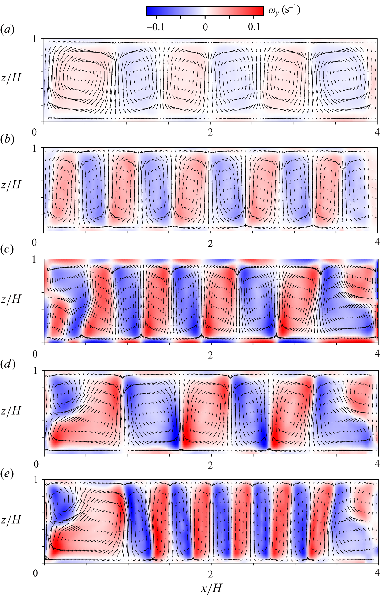
 $Pr \approx 150$. The development is represented by variations of the time-averaged field of 2-D velocity vectors
 $(u, w)$ and vorticity
 $\omega _y = \partial u/\partial z - \partial w/\partial x$ measured experimentally (figure 2). Note that the number of vectors displayed is reduced for better visibility. For small
 $Ra$ (
 $Ra = 1.6 \times 10^5$), fully steady convection rolls emerge (figure 2a), even though
 $Ra$ is sufficiently large to induce unsteady motions in unconfined systems. Increasing
 $Ra$ to
 $4.8 \times 10^5$, the convection rolls reduce horizontal size (or increase the horizontal wavenumber) while keeping the steadiness (figure 2b). Recall that these
 $Ra$ conditions are expected to induce strong unsteadiness for RB convection without tight lateral confinement (Krishnamurti Reference Krishnamurti1970a,Reference Krishnamurtib), suggesting that the confinement suppresses the convective motions to evolve as expected Shishkina (Reference Shishkina2021). Small rolls emerge at the corners of the fluid layer at
 $Ra = 6.7 \times 10^5$ (figure 2c). The corner rolls accompany periodic oscillations in both time and space as a result of competition between upward and downward flows detached from the bottom and top boundaries along both sidewalls. Notably, the rolls in the interior remain steady, and the unsteadiness appears locally as the oscillatory corner rolls (OCRs). We remark that the OCRs sometimes form without entailing unsteadiness, but start oscillating after a sufficiently long time, at least 30 min for all conditions explored in the experiments. The emergence of corner rolls always involves unsteadiness, and neither steady corner rolls nor unsteady vertically elongated rolls were observed. The OCRs widen their horizontal size with the increase of
 $Ra$, and so do the inner steady rolls (figure 2d). The latter is counterintuitive as a wavelength of convective structures usually decreases with the increase of
 $Ra$ irrespective of confinement (Ahlers et al. Reference Ahlers, Grossmann and Lohse2009; Hewitt et al. Reference Hewitt, Neufeld and Lister2012; Ulloa & Letelier Reference Ulloa and Letelier2022; Noto, Ulloa & Letelier Reference Noto, Ulloa and Letelier2023c). With further increase of
 $Ra$, at
 $Ra = 2.4 \times 10^6$ (figure 2e), the OCRs maintain, and the steady rolls in the interior reduce their horizontal size similar to the development at lower
 $Ra$ shown in figures 2(a,b). This widening and shrinking at higher
 $Ra$ is related to the 3-D flow development and will be discussed further in § 4.2.
Time-averaged distributions of velocity vectors and vorticity representing a development of convective flow structures with respect to  $Ra$ values (a)
 $1.6 \times 10^5$, (b)
 $4.8 \times 10^5$, (c)
 $6.7 \times 10^5$, (d)
 $1.3 \times 10^6$, and (e)
 $2.4 \times 10^6$.
To examine the time variation of the OCRs, a spatiotemporal distribution of horizontal velocity component  $u(x)$ at
 $z = 0.75H$ (figure 3), which is extracted from the time series of the 2-D velocity vector field, is shown in figure 2(d). This representation clarifies the coexistence of OCRs at the sidewalls and steady rolls in the interior as mentioned above. The diagram also indicates that the oscillations of both corner rolls do not synchronise and have individual oscillation frequencies. The frequency takes values from 0.005 to 0.01 Hz, and increases with
 $Ra$. The frequency is of the same order as the inverse of the circulation time of the laterally elongated rolls adjoining the corner rolls, and is consistent with values observed in Koster, Ehrhard & Müller (Reference Koster, Ehrhard and Müller1986) and Noto et al. (Reference Noto, Letelier and Ulloa2024). Summarising the results mentioned above, the regime of OCRs is qualitatively the same as that reported by Koster et al. (Reference Koster, Ehrhard and Müller1986).
A spatiotemporal distribution of velocity component  $u$ extracted along the horizontal line at
 $z/H = 0.75$ from figure 2(d).

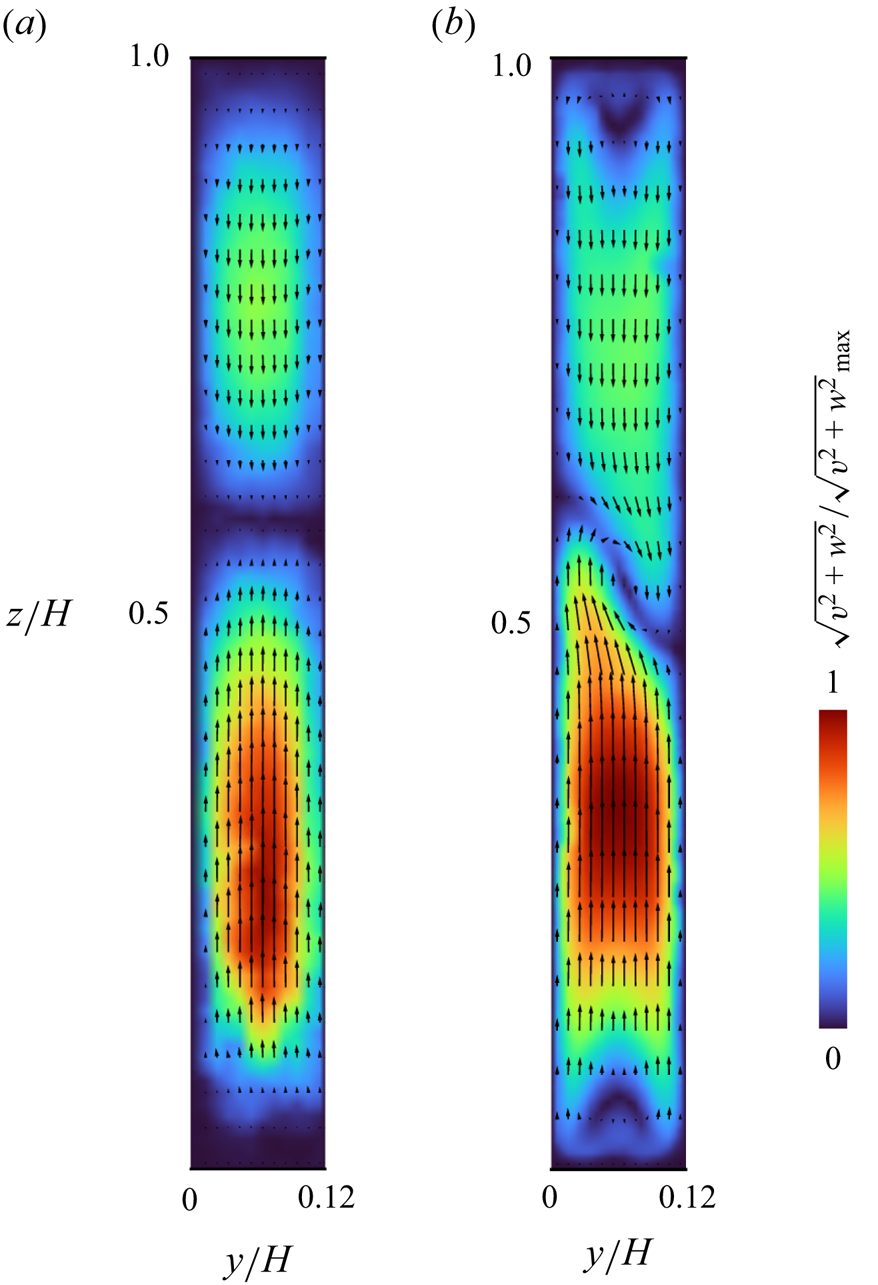
To characterise the flow structures experiencing the aforementioned transitions further, we also perform PIV measurements on a cross-section along the  $y$ direction. Assuming that the confinement is tight enough, Poiseuille flow is expected to form within the Hele-Shaw geometries; otherwise, such a parabolic profile will distort for loose confinement. Instantaneous velocity vector fields shown in figure 4 display the velocity field measured at
 $x/H = 0.08$, with
 $Ra = 6.7\times 10^{5}$ (figure 4a), the same condition as in figure 2(c), i.e. right after the onset of OCR formation, and
 $Ra = 1.7 \times 10^6$ (figure 4b), corresponding to the condition between figures 2(d,e). Note that this cross-section was chosen since the gapwise flow structures are expected to exhibit noticeable differences at the positions of the OCRs as the interior remains steady. The colour contour behind the vectors represents the magnitude of the velocity vectors,
 $(v^2+w^2)^{1/2}$, normalised by its maximum value in the field. The velocity distribution in figure 4(a) illustrates a symmetric, quasi-parabolic distribution,
 $|v| \approx 0$, across the
 $y$ axis at any height, representing the Poiseuille flow though small imperfections due to measurement error recognisable at the bottom wall. Meanwhile, the Poiseuille flow is perturbed at the higher
 $Ra$ as shown in figure 4(b). The velocity distribution seems symmetric in the
 $y$ direction near the top and bottom boundaries. The profile is, however, not entirely parabolic, unlike figure 4(a), exhibiting a skewed 3-D flow structure at the centre. In summary, these results suggest that the OCRs are characteristic features observed in convection in Hele-Shaw geometries, and they can be either quasi-2-D (Poiseuille flow) or 3-D (non-Poiseuille flow), depending on
 $Ra$. This will be discussed further with the results of DNS in § 3.3.
Instantaneous velocity vector fields on a  $y$–
 $z$ cross-section at
 $x/H = 0.08$: (a) at
 $Ra = 6.7 \times 10^5$, (b) at
 $Ra = 1.7 \times 10^6$, where the colour contour represents the absolute value of 2-D velocity vectors
 $(v, w)$ normalised by their maximum value in each field.
The transition from the fully steady roll regime to the OCR regime is also observed in the experiments with different  $\varGamma _y$. All experimental conditions are summarised on a
 $Ra$–
 $\varGamma _y$ parameter space to construct a regime diagram (figure 5). The black solid line indicates the critical condition of RB convection with lateral wall confinement,
 \begin{equation} Ra_{c,\varGamma} \approx (2{\rm \pi})^4 \left(1+\frac{1}{\varGamma_x^2}\right) \left(1+\frac{1}{4 \varGamma_x^2}+\frac{1}{4 \varGamma_y^2}\right), \end{equation}
presented by Shishkina (Reference Shishkina2021) with  $\varGamma _x = 4$. Beneath the line, convection does not occur, and thermal conduction state is maintained. The blue squares indicate the fully steady roll regime, and orange symbols (diamonds and triangles) represent the OCR regime. The labels from (a) to (e) correspond to the conditions shown in figure 2. In the series of plots for the OCR regime, we change the symbols from diamonds to triangles, corresponding to before and after the widening of inner rolls shown respectively in figures 2(c,d). The meaning of this counterintuitive transition will be explained later. The red line in figure 5 is drawn along the criteria of partially 3-D convection proposed by Noto et al. (Reference Noto, Letelier and Ulloa2024),
 \begin{equation} \varGamma_y = (2c\varLambda\,Pr^{\beta}\,Ra^{\gamma})^{-1}, \end{equation}
with the coefficients  $c = 0.14$,
 $\beta =-0.03$ and
 $\gamma = 0.297$ originated from
 $Nu$ scaling (Xia et al. Reference Xia, Lam and Zhou2002) and
 $\varLambda = 1/2$. Leaving from the line towards the bottom left (smaller
 $\varGamma _y$ and
 $Ra$) approaches quasi-2-D convection, where Poiseuille flow is observed across the gap, transitioning from the Hele-Shaw regime to the fully conduction regime through the Darcy regime. On the other end towards the top right (larger
 $\varGamma _y$ and
 $Ra$), the system becomes fully 3-D convection through a partially 3-D regime where the 3-D structures are localised at the horizontal boundaries (Noto et al. Reference Noto, Letelier and Ulloa2024). The star indicates the condition at which Koster et al. (Reference Koster, Ehrhard and Müller1986) observed the OCRs, close to the OCR regime in the present study.
Regime diagram and plots of the present conditions examined on the  $Ra$–
 $\varGamma _y$ plane. Blue squares correspond to the steady rolls, and the orange symbols, both diamonds and triangles, are the OCRs. The diamonds and triangles indicate the regimes without and with widening the inner rolls along the increase of
 $Ra$. The black line indicates critical Rayleigh number
 $Ra_{c, \varGamma }$ depending on
 $\varGamma _y$ in confined RB convection given by Shishkina (Reference Shishkina2021) with
 $\varGamma _x = 4$. Labels (a) to (e) indicate the conditions corresponding to the velocity distributions shown in figure 2. The red line indicates the boundary between quasi-2-D and 3-D flows for turbulent convection proposed by Noto et al. (Reference Noto, Letelier and Ulloa2024), i.e. (3.2) with the degree of confinement
 $\varLambda = 1/2$. The star indicates the condition at which Koster et al. (Reference Koster, Ehrhard and Müller1986) observed the OCRs.

3.2. Influence of width aspect ratio and Prandtl number
The OCRs formed in the fluid layer with  $\varGamma _x = 4$ (figures 2c–e) appear to span up to
 $\approx 0.5H$ in the
 $x$ direction, suggesting that
 $\varGamma _x$ plays a significant role in the formation of the OCRs. We thus examine the influence of width aspect ratio
 $\varGamma _x$. Furthermore, the dynamics may change depending on the strength of the inertial effect in the system. Here, we also investigate
 $Pr$ dependence by changing the test fluid.
Time-averaged distributions of 2-D velocity vectors and vorticity are obtained by the PIV measurements under the common conditions  $Ra = 1.3 \times 10^6$,
 $\varGamma _y = 0.12$ and
 $Pr \approx 150$, for
 $\varGamma _x=2$ in figure 6(a) and
 $\varGamma _x=1$ in figure 6(b). At
 $\varGamma _x = 2$, both the OCRs at the sidewalls and the steady rolls in the interior emerge analogously with
 $\varGamma _x = 4$. In comparison with figure 2(c), no essential difference is observed at
 $\varGamma _x = 2$ besides the difference in the size of the rolls. The flow field shown in figure 6(b) for
 $\varGamma _x = 1$ does not exhibit the inner steady rolls, but the OCRs take place in the entire domain. The latter is consistent with the previous experimental and numerical works (Ozawa et al. Reference Ozawa, Müller, Kimura and Takamori1992; Babushkin et al. Reference Babushkin, Glazkin, Demin, Platonova and Putin2009; Chong et al. Reference Chong, Wagner, Kaczorowski, Shishkina and Xia2018). Positions of the corner rolls vary in each experiment, either at the top or bottom corner, but tend to be the top corner in most of the experiments for
 $\varGamma _x = 4$. Experimental parameters examined for different
 $\varGamma _x$ are organised in the regime diagram shown in figure 6(c). The diagram indicates that the OCRs emerge at the same range of
 $Ra$, i.e.
 $Ra \approx 6.5 \times 10^5$, without strong dependence of
 $\varGamma _x$. These results suggest that the existence of the no-slip sidewalls (more strictly, say, the existence of the corner) is more essential than
 $\varGamma _x$ for the emergence of the OCRs.
Examples of time-averaged velocity vector fields corresponding to the OCR regime at (a)  $\varGamma _x = 2$ and (b)
 $\varGamma _x = 1$ under the common Rayleigh number
 $Ra = 1.3 \times 10^6$. Regime diagrams on (c)
 $\varGamma _x$–
 $Ra$ and (d)
 $Pr$–
 $Ra$ parameter spaces.

The influence of  $Pr$ is examined by varying the concentrations of xanthan gum solutions as described in § 2.1 (
 $Pr = 40$,
 $150$ and
 $750$) for
 $\varGamma _y = 0.12$ and
 $\varGamma _x = 1$. Results based on the PIV measurement are summarised in a regime diagram shown in figure 6(d). For sufficiently large
 $Pr$ (
 $Pr \geq O(10^1)$), although the flow structures are dependent on
 $Pr$, the heat transport characteristics are regardless of
 $Pr$ in unconfined systems (Schmalzl, Breuer & Hansen Reference Schmalzl, Breuer and Hansen2002; Pandey, Verma & Mishra Reference Pandey, Verma and Mishra2014). In confined systems, the diagram shown in figure 6(d) clarifies the negligible contribution of
 $Pr$ even in the flow structures, i.e. the emergence of the OCRs. Such an insensitivity to
 $Pr$ unique in confined systems suggests adequacy for adopting the infinite
 $Pr$ assumption for the DNS described in the next subsection.
3.3. Flow fields represented by numerical simulations
Numerical simulations are performed to support interpretations obtained through the laboratory experiments. Figure 7 shows time-averaged flow fields from the DNS represented in the same manner as in figure 2; in-plane velocity vectors  $(u,w)$ and out-of-plane vorticity
 $\omega _y$ at the middle vertical plane in the
 $y$ direction are superposed. For reference,
 $\omega _y$ of 2000 in the DNS approximately corresponds to 0.08 s
 $^{-1}$ in the experiments. As mentioned in § 2.2 and discussion of its adequacy in § 3.2, infinite
 $Pr$ is assumed. Figures 7(a,b) illustrate the steady roll regime where the number of rolls increases with
 $Ra$. Figure 7(c) is the case with OCRs. Figure 7(d) is also the case with OCRs, while the number of inner rolls is reduced as observed in the experiments. In figure 7(e), there still exist OCRs, but the horizontal size of inner rolls decreases again. All of these features observed in the DNS successfully reproduce the flow patterns in the experiments (figures 2a–e).
(Simulation.) Time-averaged distributions of velocity vectors and vorticity assuming infinite Prandtl number for  $\varGamma _y = 0.12$ at different Rayleigh numbers: (a)
 $1.0 \times 10^5$, (b)
 $4.0 \times 10^5$, (c)
 $6.0 \times 10^5$, (d)
 $2.0 \times 10^6$, and (e)
 $4.0 \times 10^6$.

We investigate higher  $Ra$ conditions that are difficult to attain in the experiments due to the limitation of the imposed temperature difference. The
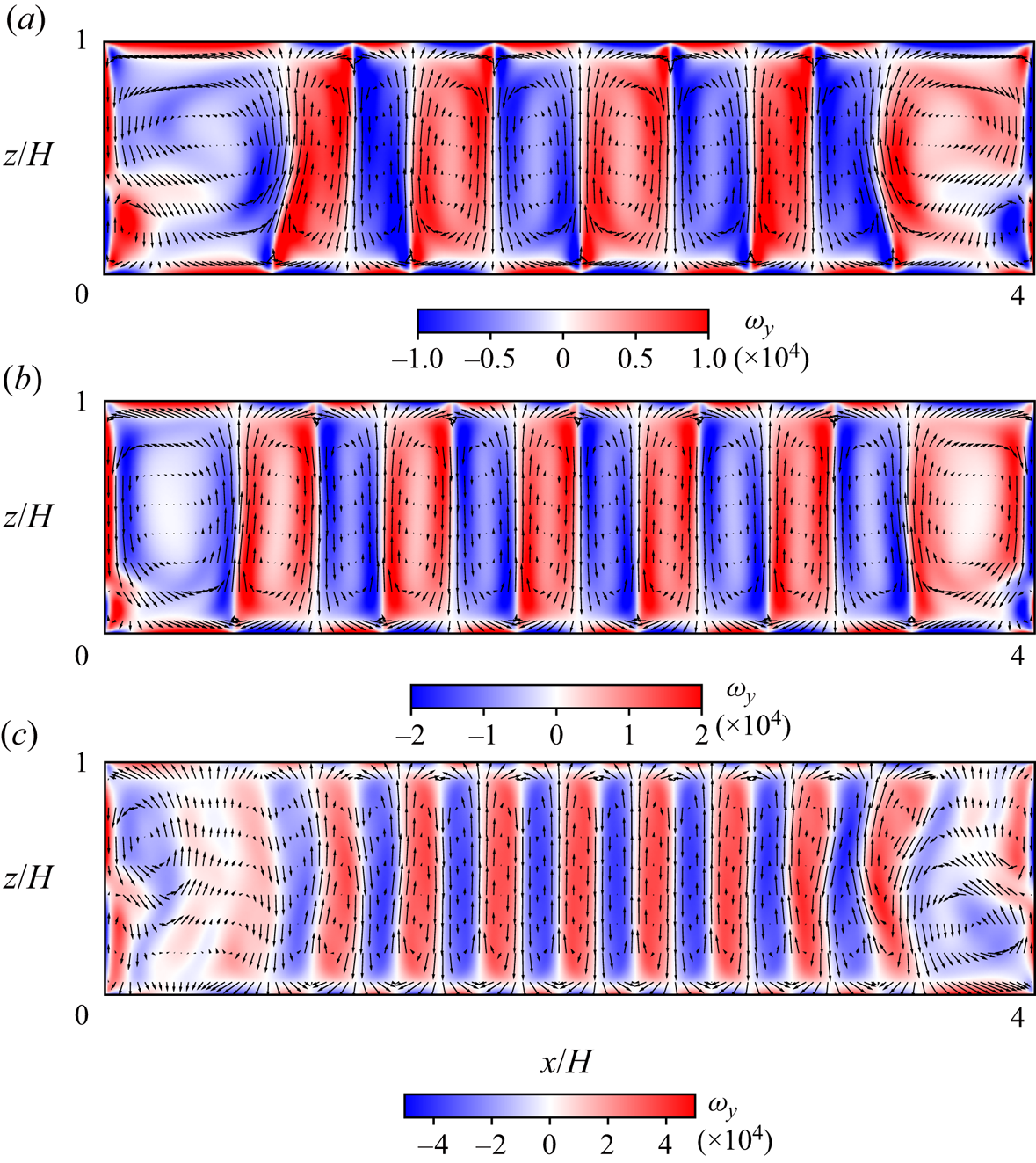
 $Ra = 1.0 \times 10^7$ shown in figure 8(a) is fully steady again even at the corner rolls, and the number of inner rolls is reduced compared to figure 7(e). The latter reappeared steady states are found for
 $Ra \geq 6.0 \times 10^6$, beyond the present experimental limit. For
 $Ra = 2.0 \times 10^7$ (figure 8b), the number of inner rolls increases again, yet the flow remains steady. Figure 8(c) uses the highest
 $Ra$ in our simulation, showing unsteady motions of plumes near the sidewalls with slight movement of inner rolls. This type of time-dependent behaviour is found for
 $Ra \geq 4.0 \times 10^7$.
(Simulation.) Time-averaged distributions of velocity vectors and vorticity assuming infinite Prandtl number for  $\varGamma _y = 0.12$ at different Rayleigh numbers: (a)
 $1.0 \times 10^7$, (b)
 $2.0 \times 10^7$, and (c)
 $6.0 \times 10^7$.
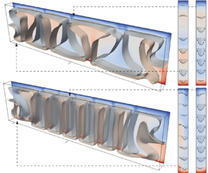
All the conditions illustrated in figures 7 and 8 are now shown altogether as 3-D perspective views in figure 9 to grasp the flow dimensionality. Each plot displays instantaneous non-dimensional temperature isosurfaces  $T = 0.45$ and
 $0.55$, together with the temperature distribution at the back wall. To the right of the 3-D views, velocity vectors and temperature distributions are shown for the
 $y$–
 $z$ cross-sections at
 $x/H = 0.25$ and
 $2.0$, indicated by ticks on the 3-D views. The flow structures are quasi-2-D for figures 9(a–d); the isosurfaces of temperature are flat in the
 $y$ direction, i.e.
 $\partial T/\partial y \approx 0$, and the velocities in the
 $y$–
 $z$ planes are parabolic,
 $|v| \approx 0$. Figures 9(a,b) show fully steady rolls, whereas figures 9(c,d) are cases with OCRs.
(Simulation.) Perspective views of instantaneous temperature isosurfaces of  $T=0.45, 0.55$ for
 $\varGamma _x = 0.12$ at different
 $Ra$: (a)
 $1.0 \times 10^5$, (b)
 $4.0 \times 10^5$, (c)
 $6.0 \times 10^5$, (d)
 $2.0 \times 10^6$, (e)
 $4.0 \times 10^6$, (f)
 $1.0 \times 10^7$, (g)
 $2.0 \times 10^7$, and (h)
 $6.0 \times 10^7$. Extracted
 $y$–
 $z$ cross-sections of temperature at
 $x/H=0.25, 2.0$ are also presented, with velocity vectors on them.

Figures 9(e–h) exhibit 3-D flow structures. The OCRs are still present in figure 9(e), showing counter-currents within the gap that reflect a deviation from the Poiseuille flow. Unlike the asymmetric velocity profile in the corner roll, the inner roll shows a nearly symmetric profile in the  $y$ direction. Figure 9(f) is the reappeared steady state at higher
 $Ra$ where the corner rolls do not oscillate. The 3-D features appear as alternate alignments of cold downward and hot upward flows on the front and back walls, respectively. That is, the quasi-2-D rolls formed at lower
 $Ra$ orient diagonally. As a result, a considerable amount of the flow component in
 $y$ direction is visible in the
 $y$–
 $z$ cross-sections, together with winding temperature distribution. The reappeared steadiness results from the avoidance of collision between upward and downward flows at sidewalls as counter-currents within the gap. If we observe this situation on the middle
 $x$–
 $z$ plane as in figures 2, 7 and 8, then the pattern seems to be compatible with quasi-2-D steady corner rolls, but the substance is the 3-D flow structure in the
 $y$ direction. Figure 9(g) is also the 3-D steady state, while the number of inner rolls increases. The structures formed in these conditions can be understood as 3-D convective cells, rather than quasi-2-D rolls. When
 $Ra$ is increased to
 $4.0 \times 10^7$, the time dependency appears again; figure 9(h) shows the time-dependent 3-D pattern with winding isosurfaces of temperature near sidewalls due to unsteady plumes and slightly swinging inner rolls. The latter is not spontaneous, but a result of lateral propagation of unsteady plumes. Concerning the development of OCRs with respect to
 $Ra$, Koster et al. (Reference Koster, Ehrhard and Müller1986) mentioned that it does not exhibit nonlinear development of the oscillation, unlike usual flow transition along the bifurcation scenario, but restores a steady state. While they did not mention the 3-D development of the pattern, the key mechanism for the transition is the deviation from the Poiseuille flow at higher
 $Ra$, as we elucidated here.
As tested in the experiments (figure 6),  $\varGamma _x$ dependence is examined also in the numerical simulation, with more variations in
 $\varGamma _x$ for
 $\varGamma _y = 0.12$ and
 $Ra = 1.0 \times 10^6$. In figure 10, the flows are expressed by
 $\omega _y$ in the middle
 $x$–
 $z$ cross-section (blue indicates anticlockwise circulation, red indicates clockwise circulation). In figure 10(a), corner rolls having the same intensity exist at each corner while keeping a steady state. Figure 10(b) is the case composed of just pairs of OCRs, while figure 10(c) has the inner region with slender rolls, analogous to those observed in the experiment (figure 6). Common in figures 10(c–e), the horizontal scale of the area under the influence of sidewalls is
 ${\sim } H/2$, and the horizontal scale of each inner roll
 ${\sim } H/4$.
(Simulation.) Time-averaged vorticity fields for  $Ra = 1.0 \times 10^6$ and
 $\varGamma _y = 0.12$ at different width aspect ratios
 $\varGamma _x$: (a)
 $0.5$, (b) 1, (c) 2, (d) 4 and (e) 8. Fields (f) and (g) are also for
 $\varGamma _x = 4$, but with a free-slip boundary at the right-hand side and both sides as indicated by broken lines.

To investigate the influence of the sidewall, we conduct simulations with free-slip boundary condition at the right side (figure 10f), and both left and right sides (figure 10g) as expressed by vertical broken lines. Corner rolls emerge only on the left sidewall in figure 10(f), and do not emerge on both sidewalls in figure 10(g). These results prove that corner rolls are maintained by no-slip sidewalls.
4. Discussions
4.1. Emergence of OCRs
The first regime transition observed in both the experiments and the simulations is from the fully steady roll regime to the OCR regime. We discuss the mechanism of emergence of the OCRs in this subsection. There are two important facts for the discussion: (1) the OCRs appear as quasi-2-D flows; and (2) the channel Reynolds number estimated from the maximum vertical velocity  $Re = w_{max} D / \nu$ is less than unity at the maximum. The former suggests that the emergence of corner rolls is important in causing the unsteadiness in quasi-2-D flows, and the latter indicates that the unsteadiness is not from the inertia effect. The existence of the sidewalls causes a larger velocity gradient near there, and the resulting pressure gradient forms corner rolls even without the inertia effect. Such corner rolls are also observed in other confined RB systems even though these have not been discussed as main issues.
Here, we call governing equations of quasi-2-D confined convection – derived in Letelier et al. (Reference Letelier, Mujica and Ortega2019) by the perturbation method considering Hele-Shaw approximation – the Poiseuille-like velocity profile in the gap with no-slip and adiabatic boundary conditions. The equations below are the vertical components of the equation of motion and heat transport equation:
 $$\begin{gather} \epsilon^2\,\frac{Ra_D}{Pr}\,\frac{\textrm{D}w}{\textrm{D}t} = \frac{\partial p}{\partial z} + T + \frac{\partial^2 w}{\partial y^2} + \epsilon^2\left(\frac{\partial^2 w}{\partial x^2} + \frac{\partial^2 w}{\partial z^2}\right), \end{gather}$$
 $$\begin{gather}\epsilon^2\,Ra_D\,\frac{\textrm{D}T}{\textrm{D}t} = \epsilon^2 \left(\frac{\partial^2 T}{\partial x^2} + \frac{\partial^2T}{\partial z^2}\right) + \frac{\partial^2T}{\partial y^2}, \end{gather}$$
where  $\mathrm {D}/\mathrm {D}t= \partial /\partial t + u\partial /\partial x + v\partial /\partial y + w\partial /\partial z$ denotes material derivative, and
 $Ra_D = g\alpha \,\Delta T\,KH/(\kappa \nu ) = Ra\,\varGamma _y^2/12$ is the Rayleigh–Darcy number with permeability
 $K = D^2/12$. Terms with
 $\epsilon ^2$ (where
 $\epsilon$ is the anisotropy ratio defined by
 $\epsilon = \sqrt {K}/H$) represent perturbation from quasi-2-D convection. Neglecting these terms from the equations above and integrating them in the
 $y$ direction, we recover Darcy equations (Hewitt et al. Reference Hewitt, Neufeld and Lister2012). In the parameter regions that we examined, the inertia term in (4.1) contains
 $\epsilon ^2\,Ra_D \approx 1$ and
 $Pr \gg 1$, so the order of the inertia term is
 $O(Pr^{-1})$. This evaluation is consistent with the small Reynolds number estimated as
 $Re < 1$. This is the reason why the nonlinear development of the oscillatory flow is not exhibited in the present system, unlike the usual flow transitions for RB convection (Krishnamurti Reference Krishnamurti1970a,Reference Krishnamurtib). Meanwhile, in the heat transport equation (4.2), the order of the unsteady term is evaluated as
 $\epsilon ^2\,Ra_D \approx 1$ and is not affected by
 $Pr$. A sufficiently large temperature gradient in the corner rolls may induce unsteadiness via the heat transport equation, like mantle convection that assumes infinite
 $Pr$.
4.2. The 3-D development
The second regime transition is distinguished by the formation of 3-D structures, and here we discuss its details. Summing up the results of the experiments and the numerical simulations describes the transition process of the convection from the quasi-2-D flow. Typical changes observed in the flow field along the flow transition with respect to  $Ra$ are the width variation of the inner convection rolls and the emergence of the OCRs. The width variation with respect to
 $Ra$ is not monotonic; the size tends to decrease, but once increases (figures 2 and 7), unlike the usual RB convection at which the width increases monotonically with respect to
 $Ra$ as a characteristic of supercritical convections in finite fluid layers (e.g. Koschmieder Reference Koschmieder1993; Hartlep, Tilgner & Busse Reference Hartlep, Tilgner and Busse2003). The variation seems to be irrespective of the emergence of the OCRs. Flow field observations in the
 $y$–
 $z$ cross-section (figures 4 and 9) indicate that restoring ‘fat’ inner rolls is followed by 3-D development of the flow deviating from Hele-Shaw approximation. Distinct 3-D development is observed with the second thinning of the inner rolls, as shown in figure 9(e): the flow takes a velocity component in the
 $y$ direction and is no longer the simple Poiseuille flow, thus motions of fluid particles are allowed to take 3-D trajectories.
We revisit the regime diagram shown in figure 5, where the different shape of symbols for the OCR regime, diamonds and triangles, indicate without or with the experience of widening of inner rolls with the increase of  $Ra$. According to the discussion above, the boundaries between the different symbols on the diagram correspond to the deviation from quasi-2-D flow towards 3-D flows. In the figure, the red line indicates the boundary between 2-D and 3-D flows drawn along a criterion
 $\varLambda = 1/2$ proposed by Noto et al. (Reference Noto, Letelier and Ulloa2024). This means that the thickness of plumes formed in ‘unconfined’ RB convection for a given
 $Ra$ and
 $Pr$ condition is half of the layer thickness, resulting in counter-currents within the gap. The predicted line places around the regime borders distinguished from the experiment. This suggests that the applicable range of the criterion is widely spread for relatively smaller
 $Ra$, where no strongly turbulent convection occurs under an unconfined scenario.
In the further development of the 3-D flows with respect to  $Ra$, the convection recovers the steady flow state as explained in § 3.3. This phenomenon was also reported in Koster et al. (Reference Koster, Ehrhard and Müller1986) for
 $Ra \sim 7 \times 10^6$ in the geometry of
 $\varGamma _y = 0.102$. The 3-D development modifies the assumptions of quasi-2-D flow mentioned above, and the upward and downward flows along the side boundaries have sufficient space in the
 $y$ direction to pass each other. Similar OCRs were also found in Noto et al. (Reference Noto, Letelier and Ulloa2024) for higher
 $Ra$ with smaller
 $\varGamma _y$ and
 $Pr$, but they did not report recovering steady state. This difference may be due to the difference in
 $Pr$, which is approximately 7–80 in Noto et al. (Reference Noto, Letelier and Ulloa2024), while Koster et al. (Reference Koster, Ehrhard and Müller1986) employed 235 in their experiments, and we assume infinite in the numerical simulation. The lateral confinement effectively augments
 $Pr$, weakening the inertial effect. The other potential reason may be the range of
 $Ra$. Noto et al. (Reference Noto, Letelier and Ulloa2024) considered
 $Ra$ values higher than those in the present study, and their systems become entirely unsteady, unlike the localised unsteadiness in the present study. Since the localisation does not happen for higher
 $Ra$, the steady 3-D regime does not appear. In other words, the localisation of unsteadiness is the key to the re-emergence of steady 3-D structures.
In summary, the flow transitions observed in the present study are within a ‘quasi-steady’ condition, i.e. unsteadiness appears locally accompanied by corner rolls, but the interior remains steady. The oscillatory motion of the corner rolls can propagate the inner region; however, the inner rolls do not exhibit spontaneous unsteady motions. In addition, the lateral confinement effectively reinforces  $Pr$, suppressing the inertial term yielding global unsteady motions.
4.3. Heat and momentum transport characteristics
Finally, we discuss heat and momentum transport characteristics by investigating variations of the Nusselt number  $Nu$, and the root mean square (r.m.s.) velocities for the entire volume. Time-averaged values of the Nusselt number are calculated both at the top boundary
 $Nu_{top}$ and at the bottom boundary
 $Nu_{bot}$:
 \begin{equation} Nu_{top}=-\left \langle \left (\frac{\partial T}{\partial z} \right)_{z=1} \right \rangle_{S, t}, \quad Nu_{bot}=-\left \langle \left(\frac{\partial T}{\partial z} \right)_{z=0} \right \rangle_{S, t}, \end{equation}
where  $\langle \cdot \rangle _{S, t}$ stands for the time–surface average on the top or bottom boundary. When thermally balanced states are achieved after adequate time integration,
 $Nu_{top} \approx Nu_{bot}$. Hence we use
 $Nu_{top}$ as
 $Nu$. The dependence of
 $Nu$ on
 $Ra$ is shown in figure 11(a) from our numerical simulations for
 $\varGamma _x = 4.0$ and
 $\varGamma _y = 0.12$. First, the plot at the smallest
 $Ra = 3.00 \times 10^4$, which is less than the critical
 $Ra_{c, \varGamma } = 3.04 \times 10^4$ predicted by (3.1), takes value unity (conduction state). At the second smallest value
 $Ra = 4.00 \times 10^4$, convection occurs as indicated by
 $Nu > 1$. The
 $Nu$ value increases with respect to
 $Ra$ by enhancement of the flow and the thinning of convection rolls. The variation changes abruptly, and its slope becomes large at
 $Ra = 3.0 \times 10^6$. This condition corresponds to the boundary between the quasi-2-D flow and the 3-D flow, which can be distinguished by the flow fields in the
 $y$–
 $z$ cross-section (figure 9). The heat transport is therefore reinforced by the 3-D development of the convection. Note that the relationship between
 $Ra$ and
 $Nu$ cannot be expressed by a simple scaling law
 $Nu \propto Ra^\gamma$ due to these transitions. However, it has been shown that the scaling depends on
 $\varGamma _y$, i.e.
 $\gamma = f(\varGamma _y)$, in confined convection (Chong & Xia Reference Chong and Xia2016; Letelier et al. Reference Letelier, Mujica and Ortega2019; Noto et al. Reference Noto, Letelier and Ulloa2024). For reference, we illustrate with a dotted line the slope of
 $Nu \propto Ra^\gamma$ with
 $\gamma = 0.35$ predicted by the empirical formula obtained in Letelier et al. (Reference Letelier, Mujica and Ortega2019),
 $\gamma (\varGamma _y) = 0.66 - 0.34\tanh [1.56\log _{10}(\varGamma _y) + 2.98]$. Overall, the slope accords with the obtained
 $Nu$–
 $Ra$ trend, except for the
 $Ra$ range with the OCRs, where the obtained
 $Nu$ drops from the slope. The empirical scaling exponent was originally acquired for periodic boundary domains in Letelier et al. (Reference Letelier, Mujica and Ortega2019), i.e. no OCR is formed. The drop from the slope is thus explained by inefficient vertical heat transport by the OCRs, as those structures do not carry heat directly from one horizontal boundary to another, but circulate within them. In other words, the vertical heat transport is largely carried by the inner rolls, and the formation of the OCRs effectively shrinks the region with efficient vertical convective heat transport. Such an inefficiency in heat transport diminishes with the increase of
 $Ra$.
Dependence of Nusselt number calculated from numerical simulation on (a)  $Ra$ (
 $\varGamma _x = 4$), and (b)
 $\varGamma _x$ (
 $Ra = 1.0 \times 10^6$) for
 $\varGamma _y = 0.12$. The dotted line in (a) shows the slope of
 $Nu \propto Ra^{0.35}$, obtained by the empirical formula (Letelier et al. Reference Letelier, Mujica and Ortega2019).

Figure 11(b) presents the dependence of  $Nu$ on
 $\varGamma _x$ for
 $\varGamma _y = 0.12$ and
 $Ra = 1.0 \times 10^6$. Some of the points correspond to the flow patterns shown in figure 10; solid diamonds indicate the values for no-slip sidewalls, while an open diamond indicates the free-slip sidewalls as in figure 10(g). The case with the smallest
 $\varGamma _x$ has a square horizontal cross-section (
 $\varGamma _x = \varGamma _y = 0.12$); then
 $Ra$ is lower than critical for the onset of convection, which is consistent with former studies (see (3.1); Zhang & Xia Reference Zhang and Xia2023). The flow pattern for
 $\varGamma _x = 0.25$ is a steady single circulation. For the no-slip conditions (solid diamonds) of
 $\varGamma _x \geq 0.5$, the
 $Nu$ values approximately monotonically increase with
 $\varGamma _x$. As discussed above, the OCRs effectively shrink the region of efficient convective heat transport by the inner rolls, and the increase of
 $\varGamma _x$ diminishes the latter effect as the horizontal size of the OCRs does not change with
 $\varGamma _x$ (see figure 10). Accordingly,
 $Nu$ increases approximately in a monotonic manner, ultimately approaching that of free-slip sidewalls (open diamond) where no OCR forms (figure 10g). Since the total heat flux is simply expressed as a summation of the heat fluxes at the regions of the inner rolls and the OCRs, the laterally averaged
 $Nu(\varGamma _x)$ influenced by the OCRs can be decomposed into that in each region,
 $Nu_{inner}$ and
 $Nu_{corner}$. That is,
 $Nu(\varGamma _x) = (1 - 2c\varGamma _x^{-1})\,Nu_{inner} + 2c\varGamma _x^{-1}\,Nu_{corner}$, where
 $c$ is the ratio of the horizontal size of the OCR region
 $W_{OCR}$ on each sidewall to
 $H$,
 $W_{OCR} = cH$. The least squares fitting for
 $\varGamma _x \geq 2$ provides
 $c = 0.496$,
 $Nu_{inner} = 6.180$ and
 $Nu_{corner} = 4.689$. The former two coefficients agree with the qualitative observation of the horizontal size of the OCRs,
 $W_{OCR} \approx H/2$ (see figure 10), and the
 $Nu$ value obtained for the free-slip boundary,
 $Nu = 6.1985$ (open diamond). Therefore,
 $Nu_{corner}$ is estimated as
 $\approx$75 % compared to
 $Nu_{inner}$. The latter supports our discussion on the decrease in
 $Nu$ due to the OCR formation.
In the statistics of the flow velocity, we calculate the r.m.s. of the total magnitude  $U_{rms}$, and that of each direction
 $u_{rms}$,
 $v_{rms}$,
 $w_{rms}$ as follows:
 \begin{gather} U_{rms}=\sqrt{\langle {u}^2+{v}^2+{w}^2\rangle_{V, t}} , \end{gather}
 \begin{gather} {u_{rms}}=\sqrt{\langle{u}^2\rangle_{V, t}} ,\quad {v_{rms}}=\sqrt{\langle {v}^2\rangle_{V, t}} ,\quad {w_{rms}}=\sqrt{\langle {w}^2\rangle_{V, t}} , \end{gather}
where  $\langle \cdot \rangle _{V, t}$ stands for the time–volume average. As the velocity is normalised by
 $\kappa /H$, the value 100 approximately corresponds to 0.2 mm s
 $^{-1}$ when scaled to the experiment. The
 $Ra$ dependence of these values is presented in figure 12(a). All of these values increase with
 $Ra$; on the other hand,
 $v_{rms}$ is much smaller than
 $w_{rms}$ and
 $u_{rms}$, especially for
 $Ra \leq 2.0\times 10^6$. It is more marked by the ratio of
 $v_{rms}$ to
 $U_{rms}$ as in figure 12(b). An abrupt increase of the value is observed at
 $Ra = 3.0 \times 10^6$, hence we can distinguish 3-D flow from quasi-2-D flow by using this ratio. In the 3-D regime, the kinetic energy in the
 $y$ direction takes up to 1 % of the total kinetic energy as
 $v_{rms}/U_{rms} \approx 10^{-1}$. The latter is too small to consider the system isotropic 3-D, but is large enough to impact the heat transport characteristic (figure 11a).
The  $Ra$ dependence of r.m.s. values of (a) velocity components calculated from numerical simulation, and (b) fraction of r.m.s. values, for
 $\varGamma _x = 4$ and
 $\varGamma _y = 0.12$.

5. Concluding remarks
In this work, we investigated the effect of unidirectional confinement on thermal convection by laboratory experiments and direct numerical simulations (DNS) using Hele-Shaw geometries. The target parameter space of  $Pr$ and
 $Ra$ is relatively high
 $Pr$ (
 $\geq 40$), and from the onset of convection to moderate
 $Ra$,
 $Ra \leq 3 \times 10^6$ in the experiments and
 $Ra \leq 6 \times 10^7$ in the DNS. In the experiments, we quantified the velocity field by particle image velocimetry, and the flow structures are reproduced well by our DNS assuming infinite
 $Pr$. Combining the results of the experiments and DNS, the convective transitions along with the increase of
 $Ra$ can be summarised as follows: (I) quasi-2-D, steady rolls with similar size; (II) quasi-2-D, oscillatory corner rolls (OCRs) at both sidewalls and steady inner rolls; (III) 3-D, OCRs and inner rolls accompanied by weak flow in the
 $y$ (narrow) direction; (IV) 3-D, re-emergence of steady flow by avoiding collision between upward and downward flows at sidewalls; and (V) 3-D, time-dependent flow caused by rise and fall of plumes around sidewalls. In these transitions, unsteadiness is not seen in the entire volume but is limited around the sidewalls characterised by the OCRs. The essence of understanding these transitions is the development of 3-D flow, that is, deviation from Poiseuille flow in the
 $y$ direction. We considered the criterion
 $\varLambda \sim 1/2$ that explains the boundary between quasi-2-D and 3-D flow by Noto et al. (Reference Noto, Letelier and Ulloa2024), and confirmed its validity in the present conditions with higher
 $Pr$ and lower
 $Ra$ where the convective flow is not strongly turbulent. In addition, the re-emergence of the steady flow (IV) can be understood as a phenomenon that features in high-
 $Pr$ situations. Regarding (II), the OCRs around both sidewalls and the slender inner rolls always coexist for wide domains,
 $\varGamma _x \geq 2$. The horizontal scale of the region under the influence of sidewalls is less than the layer height
 $H$, and the number of inner rolls increases with
 $\varGamma _x$. We also found that the OCRs not only are relevant in the regime transitions but also weaken the total heat transport, resulting in a decrease of
 $Nu$, as these structures do not directly carry heat from one horizontal surface to another. This study has explored the complex convective regime transitions of severely confined, but laterally elongated convection of highly viscous fluids as above, deepening the fundamental fluid physics of thermal convection as well as Earth science and thermal engineering.
Acknowledgements
The authors are grateful for the helpful discussions with Dr T. Miyagoshi (JAMSTEC) and Dr H.N. Ulloa (University of Pennsylvania). Numerical simulations were performed on the Earth Simulator at JAMSTEC. This work was supported by the Joint Usage/Research Center PRIUS, Ehime University, Japan.
Funding
This work was supported by the Japan Science and Technology Agency (JST), PRESTO grant no. JPMJPR21O6.
Declaration of interests
The authors report no conflict of interest.



