



1 Introduction
In this paper, we deal with electrohydrodynamic flow (EHD), which studies the flow dynamics of fluids subject to an electric field, cf. Castellanos (Reference Castellanos1998). The flow configuration of EHD resembles Rayleigh–Bénard convection (RBC) except that, instead of a thermal gradient, it is potential difference that is imposed across two infinite plates, see figure 1 for an illustration of EHD. Unipolarly charged ions are issued from the injector towards the collector. Electric Coulomb force, as a result of the imposed potential difference, acting on the charged ions can potentially destabilize the flow and lead to flow motion; the latter in turn affects the charge distribution. As the interaction between flow field and electric field is nonlinear, problems in EHD are notoriously difficult to elucidate. On the other hand, the application potential of EHD is immense in mechanical and biological engineering, including electrostatic precipitators, microscale EHD pumps, EHD drag reduction, heat transfer enhancement by means of EHD and drug delivery systems, to name a few. It is thus interesting and important to study EHD.
In this work, a fundamental EHD problem of a simple geometry is considered; specifically, we study the weakly nonlinear stability of convective motions induced by unipolar charge injection into an insulating dielectric liquid between two parallel rigid plane electrodes, with and without cross-flow. This important problem is yet to be well explored. Moreover, as the flow setting is simple, the essential nonlinear mechanism in EHD can be better untangled, which will be important in understanding the more complicated EHD-related phenomena or designing the more sophisticated EHD-driven devices. In the following sections, stability of EHD flow is discussed.
Illustration of flow configuration for 2-D EHD flow. Black dots represent fluid particles. Circles with a positive sign are unipolarly charged ions subject to an electric field
 $E$
as a result of an imposed potential difference. Dashed grey curves with arrows denote the convection formed in hydrostatic EHD flow due to the electric Coulomb force.

1.1 Instability and bifurcation of electrohydrodynamic flow
The linear stability analysis of electrohydrodynamic flow of dielectric liquids subject to unipolar charge injection has been first studied by Schneider & Watson (Reference Schneider and Watson1970) and Atten & Moreau (Reference Atten and Moreau1972). The linear stability criterion of the stability parameter
 $T$
, the electric Rayleigh number, was established to be
 $T_{c}C^{2}\approx 220.7$
in the case of the weak-injection limit (
 $C\ll 1$
,
 $C$
is charge injection level, defined in (2.2) with
 $T$
) and
 $T_{c}\approx 160.75$
when
 $C\rightarrow \infty$
in the space-charge-limited (SCL) regime. However, the experimentally determined linear stability criterion
 $T_{c}$
was found to be approximately 100 for SCL (Atten & Lacroix Reference Atten and Lacroix1979), significantly lower than the theoretical prediction, suggesting a subcritical nature of the transition to turbulence in EHD. This discrepancy between the theory and the experiment in the SCL regime has recently been examined by Zhang et al. (Reference Zhang, Martinelli, Wu, Schmid and Quadrio2015) using modal and non-modal linear stability analysis tools (Farrell & Ioannou Reference Farrell and Ioannou1996; Schmid Reference Schmid2007) with the charge diffusion effect included. However, the authors find that the perturbation energy growth is limited in the whole linear phase; therefore, the transient growth transition mechanism is probably not the main bifurcation route for the subcritical transition in EHD flow without cross-flow.
The nonlinear stability analysis of EHD flow started with the work by Félici (Reference Félici1971). Even though the author only solved a one-way coupling system with the assumption of a two-dimensional, a priori hydraulic model for the velocity field in the weak-injection case, the subcritical feature of nonlinear EHD flow has been successfully deduced in that there exist two solutions below the linear critical criterion
 $T_{c}$
, a stable state and a finite-amplitude state. This result was further collaborated by the results in Atten & Lacroix (Reference Atten and Lacroix1974), who established the
 $(T_{c}-T)^{1/2}$
relationship of the vertical velocity maximum
 $V_{m}$
near the criticality
 $T_{c}$
and suggested the existence of a hysteresis loop in the transition of EHD to turbulence. Further development in the nonlinear stability analysis of EHD flow, for example, the pattern formation, was then discussed in Lacroix, Atten & Hopfinger (Reference Lacroix, Atten and Hopfinger1975), in which the authors found the formation of hexagonal cells as the main convective pattern in the electroconvetion and also briefly discussed the occurrence of nonlinear instability phenomena. The theoretical explanation of such pattern selection was postponed until Atten & Lacroix (Reference Atten and Lacroix1979), who performed a nonlinear stability analysis of Félici’s hydraulic model in the weak-injection case and a weakly nonlinear stability analysis of EHD flow in the SCL regime using the modal equation approximation method, arriving at the conclusions that the hexagonal cells are more stable than the 2-D rolls and that the flow inside the cells flows towards the injection electrode. The authors also reported the nonlinear stability criterion
 $T_{nl}$
for 3-D, hexagonal cells to be
 $T_{nl}\approx 90$
in the experiments, in contrast to the theoretical results
 $T_{nl}\approx 110$
.
The bifurcation of EHD flow near the linear criticality
 $T_{c}$
has also been studied using the direct numerical simulation (DNS) method, for example, in Chicón, Castellanos & Martin (Reference Chicón, Castellanos and Martin1997), Wu et al. (Reference Wu, Traoré, Vázquez and Pérez2013). In Wu et al. (Reference Wu, Traoré, Vázquez and Pérez2013), the authors investigated the EHD flow bifurcating at criticality in a 2-D finite container without considering the charge diffusion effect. In their results, the reference calculation, in which periodic boundary conditions are imposed on the vertical walls mimicking the infinite electrodes, yields the classical results of the linear stability theory and its subcritical bifurcation; whereas, in a confined container, the bifurcation might switch to a supercritical route in some parameter subspace partially owing to the dissipative effect of the vertical walls. This DNS method for bifurcation analysis is useful and convenient when a DNS solver is ready. In this regard, the more general method of performing bifurcation analysis using DNS, the time stepper method, is discussed thoroughly in Tuckerman & Barkley (Reference Tuckerman and Barkley1999).
1.2 Weakly nonlinear stability analysis
As the amplitude of the linear modes grows to some point, it is not valid any more to neglect the nonlinearity. In the research of nonlinear phenomena, much attention has been devoted to the weakly nonlinear phase around the linear criticality, as analytical modelling of the weak nonlinearity is possible. One of the well-developed theoretical tools for the study of weak nonlinearity is multiple scale analysis, which is the main mathematical tool to be employed in the present work.
In weakly nonlinear stability analysis, expansion of the disturbance terms in the Navier–Stokes (NS) equation leads to the famous Ginzburg–Landau equation (GLE), first proposed by Landau (Reference Landau1944) in the discussion of the origin of turbulence, as a universal governing equation for the disturbance amplitude around the first bifurcation. In the community of fluid mechanics, the first rigorous derivation of GLE was given by Stuart (Reference Stuart1960) for plane Poiseuille flow (PPF); at the same time, Watson (Reference Watson1960) reached the same equation using the amplitude expansion method. The multiple-scale analysis, a more general derivation scheme extending the expansion method in Stuart (Reference Stuart1960), was then proposed by Stewartson & Stuart (Reference Stewartson and Stuart1971). The ambiguity in the values of the Landau coefficients (the coefficients in GLE) obtained in the weakly nonlinear analysis was clarified by Herbert (Reference Herbert1983), Sen & Venkateswarlu (Reference Sen and Venkateswarlu1983), who proposed to fix the amplitude of the disturbance eigenfunction to be unit at the channel centreline, for example, for PPF. These two methods, the amplitude expansion method and multiple-scale analysis, are proved to be equivalent in the work by Fujimura (Reference Fujimura1989). A third alternative, the centre manifold reduction method, has also been shown to be able to arrive at the same GLE by Fujimura (Reference Fujimura1991, Reference Fujimura1997).
Other than the simplest flow configuration PPF, the weakly nonlinear stability analysis has also been applied to other complex fluids. Here, we discuss some of them which are most relevant to EHD flow. The RBC, mentioned above, has been shown to be an excellent model for the derivation of GLE as in this case, analytical expression of the Landau coefficients can be obtained when the boundary conditions are assumed to be free surfaces (also known as Bénard–Marangoni convection), see Cross (Reference Cross1980). The similar geometries and configurations between RBC and EHD tempt one to compare the two flows; however, it is well-known that the bifurcation of RBC, under the linear Oberbeck–Boussinesq approximation, is of a supercritical nature (Cross & Hohenberg Reference Cross and Hohenberg1993), which is different from the subcritical bifurcation of EHD, as discussed above. This makes the bifurcation in EHD flow interesting since the nonlinear terms in EHD flow should behave in a quite different manner than those in RBC, resulting in a different bifurcation route. Another type of fluid subject to electric field, closely related to EHD, is that of nematic liquid crystals. The amplitude equation and the pattern formation for nematic liquid crystals have been discussed by Pesch & Kramer (Reference Pesch and Kramer1986), Kramer & Pesch (Reference Kramer and Pesch1995) and more recently by Plaut et al. (Reference Plaut, Decker, Rossberg, Kramer, Pesch, Belaidi and Ribotta1997). The main dissimilar feature between the two fluids lies in the difference that the nematic liquid crystals are anisotropic with a preferred axis while the EHD flow of non-polar liquids, the working fluids that we are considering, is isotropic in all the wall-parallel directions when a constant potential difference is imposed across the infinite electrodes. Therefore, the pattern formation in nematic liquid crystals adopts more likely the form of normal rolls which is parallel or perpendicular to the preferred axis. Besides the two flow configurations just discussed, electro-thermal hydrodynamics (ETHD) is perhaps the most relevant flow related to EHD. ETHD studies the flow dynamics of fluids subject to at the same time the potential difference and a heat gradient; this combined effect is interesting because proper manipulation of the electric field can lead to increased efficiency of heat transfer, and thus imply various industrial applications. In fact, the weakly nonlinear analysis of ETHD has been performed by Worraker & Richardson (Reference Worraker and Richardson1981) following the linear stability analyses of Turnbull (Reference Turnbull1968). By deriving the Ginzburg–Landau equation until the third order, Worraker & Richardson (Reference Worraker and Richardson1981) successfully described the flow transition of ETHD from a supercritical bifurcation to a subcritical one when an electric potential of increasing strength is imposed across two differentially heated plates. This result has also been recently obtained and discussed in Traoré et al. (Reference Traoré, Párez, Koulova and Romat2010). On the other hand, in the presence of cross-flow, the weakly nonlinear analysis and the pattern selection of a heated fluid with through flow have been studied by Fujimura & Kelly (Reference Fujimura and Kelly1995), Kato & Fujimura (Reference Kato and Fujimura2000). However, there seems to be no study in the literature on weakly nonlinear EHD with cross-flow.
1.3 Present work
To further distil the flow transition and bifurcation mechanism in EHD, it is important to study in detail its nonlinear stability. On one hand, for hydrostatic EHD flow, the weakly nonlinear stability analysis by Atten & Lacroix (Reference Atten and Lacroix1979) only considered the limit of infinite
 $M$
(
 $M$
is the ratio between hydrodynamic mobility and ion mobility, introduced in (2.2) below) and the inertial terms are thus neglected following this assumption. No detailed parametric study was presented in their article. In the ETHD work by Worraker & Richardson (Reference Worraker and Richardson1981), the pure EHD flow in a weakly nonlinear phase is marginally discussed as a special case when the thermal difference
 $k_{1}$
across two plates is zero. On the other hand, EHD with cross-flow was rarely studied in the past. Linear stability of such flow has been documented in Castellanos & Agrait (Reference Castellanos and Agrait1992), Lara, Castellanos & Pontiga (Reference Lara, Castellanos and Pontiga1997), Zhang et al. (Reference Zhang, Martinelli, Wu, Schmid and Quadrio2015), but, to the best of our knowledge, weakly nonlinear stability analysis of EHD-Poiseuille flow has never been reported in the literature.
We are prompted by the consideration that a more comprehensive and accurate analysis of weakly nonlinear EHD is needed for a better understanding of such flow. Therefore, in the present work, we conduct in detail the weakly nonlinear stability analysis of 2-D EHD in the space charge limit, with and without cross-flow, by performing a multiple-scale analysis around the linear critical condition. The effect of charge diffusion, which has long been omitted since the work of Pérez & Castellanos (Reference Pérez and Castellanos1989), is taken into account for the completion of physical modelling. The EHD with cross-flow, rarely studied in the literature, is considered as it is interesting to see how the canonical channel flow can be modified due to the presence of an electric field. This would be essential for the design of certain flow control strategies employing an electric field as the manipulating agent; for example, the modification to the wake flow in a developed Poiseuille flow using the electric field (Mccluskey & Atten Reference Mccluskey and Atten1988) or turbulence modification using EHD (Soldati & Banerjee Reference Soldati and Banerjee1998). In the end, compared to Worraker & Richardson (Reference Worraker and Richardson1981), who obtained the cubic GLE, we derive the GLE until the fifth order; therefore, a stable solution to the GLE can be obtained for the subcritical EHD when the fifth-order nonlinear term stabilizes the flow.
The paper is organized as follows. In § 2, we present the governing equations and the mathematical formulation of the multiple-scale analysis. In § 3, we briefly present the numerical method. The validation and the results of weakly nonlinear EHD with and without cross-flow are shown in § 4. The results are compared to DNS and experiments whenever possible. Finally in § 5, we conclude the paper with a discussion about the results.
2 Problem formulation
2.1 Non-dimensionalized governing equations
The details of the mathematical modelling of EHD flow can be found in the classical books, such as Melcher (Reference Melcher1981), Castellanos (Reference Castellanos1998) or in our previous work Zhang et al. (Reference Zhang, Martinelli, Wu, Schmid and Quadrio2015). We present briefly the non-dimensionalized governing equations as below.
We non-dimensionalize the full system with the characteristics of electric field, i.e.
 $L^{\ast }$
(half distance between the electrodes),
 ${\rm\Delta}{\it\phi}_{0}^{\ast }$
(voltage difference applied to the electrodes) and
 $Q_{0}^{\ast }$
(injected charge density). Accordingly, time
 $t^{\ast }$
is non-dimensionalized by
 $L^{\ast 2}/(K^{\ast }{\rm\Delta}{\it\phi}_{0}^{\ast })$
, velocity
 $\boldsymbol{U}^{\ast }$
by
 $K^{\ast }{\rm\Delta}{\it\phi}_{0}^{\ast }/L^{\ast }$
, pressure
 $P^{\ast }$
by
 ${\it\rho}_{0}^{\ast }K^{\ast 2}{\rm\Delta}{\it\phi}_{0}^{\ast 2}/L^{\ast 2}$
, electric field
 $\boldsymbol{E}^{\ast }$
by
 ${\rm\Delta}{\it\phi}_{0}^{\ast }/L^{\ast }$
and electric density
 $Q^{\ast }$
by
 $Q_{0}^{\ast }$
. Therefore, the non-dimensional EHD-NS equations read
 $$\begin{eqnarray}\displaystyle & \displaystyle \boldsymbol{{\rm\nabla}}\boldsymbol{\cdot }\boldsymbol{U}=0, & \displaystyle\end{eqnarray}$$
 $$\begin{eqnarray}\displaystyle & \displaystyle \frac{\partial \boldsymbol{U}}{\partial t}+(\boldsymbol{U}\boldsymbol{\cdot }\boldsymbol{{\rm\nabla}})\boldsymbol{U}=-\boldsymbol{{\rm\nabla}}P+\frac{M^{2}}{T}{\rm\nabla}^{2}\boldsymbol{U}+CM^{2}Q\boldsymbol{E}, & \displaystyle\end{eqnarray}$$
 $$\begin{eqnarray}\displaystyle & \displaystyle \frac{\partial Q}{\partial t}+\boldsymbol{{\rm\nabla}}\boldsymbol{\cdot }[(\boldsymbol{E}+\boldsymbol{U})Q]=\frac{1}{Fe}{\rm\nabla}^{2}Q, & \displaystyle\end{eqnarray}$$
 $$\begin{eqnarray}\displaystyle & \displaystyle {\rm\nabla}^{2}{\it\phi}=-CQ, & \displaystyle\end{eqnarray}$$
 $$\begin{eqnarray}\displaystyle & \displaystyle \boldsymbol{E}=-\boldsymbol{{\rm\nabla}}{\it\phi}, & \displaystyle\end{eqnarray}$$
 $$\begin{eqnarray}M=\frac{({\it\epsilon}^{\ast }/{\it\rho}_{0}^{\ast })^{1/2}}{K^{\ast }},\quad T=\frac{{\it\epsilon}^{\ast }{\rm\Delta}{\it\phi}_{0}^{\ast }}{K^{\ast }{\it\mu}^{\ast }},\quad C=\frac{Q_{0}^{\ast }L^{\ast 2}}{{\rm\Delta}{\it\phi}_{0}^{\ast }{\it\epsilon}^{\ast }},\quad Fe=\frac{K^{\ast }{\rm\Delta}{\it\phi}_{0}^{\ast }}{D_{{\it\nu}}^{\ast }}.\end{eqnarray}$$
 $K^{\ast }$
stands for ionic mobility,
 ${\it\epsilon}^{\ast }$
represents fluid permittivity,
 $D_{{\it\nu}}^{\ast }$
is the charge diffusion coefficient and
 ${\it\mu}^{\ast }$
denotes dynamic viscosity. In (2.2),
 $M$
is the ratio between the hydrodynamic mobility
 $({\it\epsilon}^{\ast }/{\it\rho}_{0}^{\ast })^{1/2}$
and the true ion mobility
 $K^{\ast }$
.
 $T$
, the electric Rayleigh number, as mentioned in the introduction section, represents the ratio of the Coulomb force to the viscous force.
 $C$
, also appearing in the introduction section, measures the injection level.
 $Fe$
is the reciprocal of the non-dimensionalized charge diffusivity coefficient. Note that our
 $C$
, defined with respect to half-channel distance (the same as the
 $C$
in Zhang et al. (Reference Zhang, Martinelli, Wu, Schmid and Quadrio2015)), is four times the one defined according to full-channel distance, which is the usual definition of
 $C$
in previous research works on EHD (for example, our
 $C=12.5$
is actually equivalent to
 $C=50$
defined with full-channel distance); this convention is not followed here since we will also consider EHD-Poiseuille flow, and in the research of channel flow, the convention is that half-channel distance is used as the reference length. In addition, the above equations are complemented with the non-dimensionalized boundary conditions, which are
 $\boldsymbol{U}(\pm 1)=0$
,
 ${\it\phi}(1)=1$
,
 ${\it\phi}(-1)=0$
,
 $Q(1)=-1$
and
 $(\partial Q/\partial y)(-1)=0$
.
Base states for
 $\bar{{\it\phi}},\bar{E},\bar{Q},\bar{Q}C$
at
 $C=12.5,Fe=10^{5}$
(blue solid line with dots),
 $C=100,Fe=10^{5}$
(red dash-dotted line) and
 $C=12.5,Fe=10^{3}$
(black dashed line). Inset in each figure zooms in part of the figure.

The flow variables are decomposed into base states
 $(\bar{\boldsymbol{U}},\bar{\boldsymbol{E}},\bar{{\it\phi}},\bar{Q})^{\text{T}}$
as a function of
 $y$
and the perturbations
 $(\boldsymbol{u},\boldsymbol{e},{\it\varphi},q)^{\text{T}}$
as a function of
 $t,x,y$
. Superscript
 $^{\text{T}}$
denotes transpose. The base states satisfy the steady EHD-NS coupled system (2.1), which is, though not mathematically rigorous, a common practice in stability theory (Cowley & Wu Reference Cowley and Wu1994). We consider a base electric field only acting in the vertical direction
 $y$
, i.e.
 $\bar{\boldsymbol{E}}=(0,\bar{E}(y))^{\text{T}}$
. The procedure to obtain base states follows Zhang et al. (Reference Zhang, Martinelli, Wu, Schmid and Quadrio2015). Examples of
 $\bar{{\it\phi}},\bar{E},\bar{Q}$
at different
 $C$
and
 $Fe$
are shown in figure 2. It is seen that
 $C$
has a minor effect on the base profiles of
 $\bar{{\it\phi}}$
and
 $\bar{E}$
in the SCL regime, but a noticeable influence on
 $\bar{Q}$
and
 $\bar{Q}C$
; on the other hand,
 $Fe$
, representing the charge diffusion effect, apparently affects all the base profiles in the range of
 $Fe\in [10^{3},10^{5}]$
.
With the above decomposition, and after writing the electric variables in terms of
 ${\it\varphi}$
, we obtain the nonlinear governing equations for the perturbations
 $$\begin{eqnarray}\displaystyle \frac{\partial u_{i}}{\partial x_{i}} & = & \displaystyle 0,\end{eqnarray}$$
 $$\begin{eqnarray}\displaystyle \frac{\partial u_{i}}{\partial t} & = & \displaystyle -\bar{U}\frac{\partial u_{i}}{\partial x}-v\bar{U}^{\prime }{\it\delta}_{i1}-\frac{\partial p}{\partial x_{i}}+\frac{M^{2}}{T}\frac{\partial ^{2}u_{i}}{\partial x_{j}\partial x_{j}}+M^{2}\left(\bar{{\it\phi}}^{\prime \prime }\frac{\partial {\it\varphi}}{\partial x_{i}}+\bar{{\it\phi}}^{\prime }\frac{\partial ^{2}{\it\varphi}}{\partial x_{j}\partial x_{j}}{\it\delta}_{i2}\right)\nonumber\\ \displaystyle & & \displaystyle -\,u_{j}\frac{\partial u_{i}}{\partial x_{j}}+M^{2}\frac{\partial {\it\varphi}}{\partial x_{i}}\frac{\partial ^{2}{\it\varphi}}{\partial x_{j}\partial x_{j}},\end{eqnarray}$$
 $$\begin{eqnarray}\displaystyle \frac{\partial {\rm\nabla}^{2}{\it\varphi}}{\partial t} & = & \displaystyle \bar{{\it\phi}}^{\prime \prime \prime }\left(\frac{\partial {\it\varphi}}{\partial y}-v\right)+\left(\bar{{\it\phi}}^{\prime }\frac{\partial }{\partial y}-\bar{U}\frac{\partial }{\partial x}\right){\rm\nabla}^{2}{\it\varphi}+2\bar{{\it\phi}}^{\prime \prime }{\rm\nabla}^{2}{\it\varphi}+\frac{1}{Fe}{\rm\nabla}^{4}{\it\varphi}\nonumber\\ \displaystyle & & \displaystyle +\,\left(\frac{\partial {\it\varphi}}{\partial x_{i}}-u_{i}\right)\frac{\partial {\rm\nabla}^{2}{\it\varphi}}{\partial x_{i}}+{\rm\nabla}^{2}{\it\varphi}{\rm\nabla}^{2}{\it\varphi},\end{eqnarray}$$
 ${\rm\nabla}^{2}=(\partial ^{2}/\partial x^{2})+(\partial ^{2}/\partial y^{2})$
, prime denotes derivative with respect to
 $y$
and
 ${\it\delta}$
is the Kronecker delta. The Einstein summation convention is assumed in the form above. Since a 2-D problem will be considered, it is possible to express the flow velocities in terms of the streamfunciton
 ${\it\psi}$
, i.e.
 $u=(\partial {\it\psi}/\partial y),v=-(\partial {\it\psi}/\partial x)$
. Consequently, the continuity equation (2.3a
) is automatically satisfied by
 ${\it\psi}$
. Moreover, we can define the transverse vorticity
 ${\it\omega}=(\partial v/\partial x)-(\partial u/\partial y)$
which is related to
 ${\it\psi}$
by
 ${\it\omega}=-{\rm\nabla}^{2}{\it\psi}$
. By these relations, it can be shown that the system as a function of
 $(u,v)^{\text{T}}$
can be recast to one with respect to
 $({\it\omega},{\it\psi})^{\text{T}}$
. So the governing equations for the perturbations (2.3) can now be rewritten as a function of
 ${\it\gamma}=({\it\psi},{\it\varphi})^{\text{T}}$
 $$\begin{eqnarray}\displaystyle \frac{\partial {\rm\nabla}^{2}{\it\psi}}{\partial t} & = & \displaystyle -\bar{U}\frac{\partial {\rm\nabla}^{2}{\it\psi}}{\partial x}+\bar{U}^{\prime \prime }\frac{\partial {\it\psi}}{\partial x}+\frac{M^{2}}{T}{\rm\nabla}^{4}{\it\psi}-M^{2}\left(\bar{{\it\phi}}^{\prime }\frac{\partial {\rm\nabla}^{2}{\it\varphi}}{\partial x}-\bar{{\it\phi}}^{\prime \prime \prime }\frac{\partial {\it\varphi}}{\partial x}\right)\nonumber\\ \displaystyle & & \displaystyle -\,\left(\frac{\partial {\it\psi}}{\partial y}\frac{\partial {\rm\nabla}^{2}{\it\psi}}{\partial x}-\frac{\partial {\it\psi}}{\partial x}\frac{\partial {\rm\nabla}^{2}{\it\psi}}{\partial y}\right)-M^{2}\left(\frac{\partial {\it\varphi}}{\partial y}\frac{\partial {\rm\nabla}^{2}{\it\varphi}}{\partial x}-\frac{\partial {\it\varphi}}{\partial x}\frac{\partial {\rm\nabla}^{2}{\it\varphi}}{\partial y}\right),\end{eqnarray}$$
 $$\begin{eqnarray}\displaystyle \frac{\partial {\rm\nabla}^{2}{\it\varphi}}{\partial t} & = & \displaystyle \bar{{\it\phi}}^{\prime \prime \prime }\left(\frac{\partial {\it\varphi}}{\partial y}+\frac{\partial {\it\psi}}{\partial x}\right)+\left(\bar{{\it\phi}}^{\prime }\frac{\partial }{\partial y}-\bar{U}\frac{\partial }{\partial x}\right){\rm\nabla}^{2}{\it\varphi}+2\bar{{\it\phi}}^{\prime \prime }{\rm\nabla}^{2}{\it\varphi}+\frac{1}{Fe}{\rm\nabla}^{4}{\it\varphi}\nonumber\\ \displaystyle & & \displaystyle +\,\left(\frac{\partial {\it\varphi}}{\partial x}-\frac{\partial {\it\psi}}{\partial y}\right)\frac{\partial {\rm\nabla}^{2}{\it\varphi}}{\partial x}+\left(\frac{\partial {\it\varphi}}{\partial y}+\frac{\partial {\it\psi}}{\partial x}\right)\frac{\partial {\rm\nabla}^{2}{\it\varphi}}{\partial y}+{\rm\nabla}^{2}{\it\varphi}{\rm\nabla}^{2}{\it\varphi}.\end{eqnarray}$$
 ${\it\psi}$
and
 ${\it\varphi}$
are homogeneous
 $$\begin{eqnarray}\displaystyle & \displaystyle {\it\psi}(\pm 1)={\it\psi}^{\prime }(\pm 1)=0, & \displaystyle\end{eqnarray}$$
 $$\begin{eqnarray}\displaystyle & \displaystyle {\it\varphi}(\pm 1)={\it\varphi}^{\prime \prime }(1)={\it\varphi}^{\prime \prime \prime }(-1)=0. & \displaystyle\end{eqnarray}$$
 $$\begin{eqnarray}\unicode[STIX]{x1D648}\frac{\partial {\it\gamma}}{\partial t}=\unicode[STIX]{x1D647}{\it\gamma}+\unicode[STIX]{x1D649}\quad \text{or}\quad \left(\unicode[STIX]{x1D648}\frac{\partial }{\partial t}-\unicode[STIX]{x1D647}\right){\it\gamma}=\unicode[STIX]{x1D649},\end{eqnarray}$$
where the operators
 $\unicode[STIX]{x1D648},\unicode[STIX]{x1D647},\unicode[STIX]{x1D649}$
represent the weight matrix, the linear operator and the nonlinear operator, respectively. Their expressions can be easily deduced according to (2.4).
2.2 Weakly nonlinear stability analysis
To study the weakly nonlinear stability of EHD, we employ the multiple scale analysis first introduced in Stewartson & Stuart (Reference Stewartson and Stuart1971) for fluid dynamists. The procedures begin with expanding the parameters and the disturbance variables in ascending powers of a small dimensionless parameter
 ${\it\epsilon}$
(not to be confused with
 ${\it\epsilon}^{\ast }$
, the fluid permittivity, introduced above). Firstly, we assume that the time and the space scales can be expanded as
 $$\begin{eqnarray}\displaystyle & \displaystyle \frac{\partial }{\partial t}=\frac{\partial }{\partial t_{0}}+{\it\epsilon}\frac{\partial }{\partial t_{1}}+{\it\epsilon}^{2}\frac{\partial }{\partial t_{2}}+{\it\epsilon}^{4}\frac{\partial }{\partial t_{4}}+O({\it\epsilon}^{5}), & \displaystyle\end{eqnarray}$$
 $$\begin{eqnarray}\displaystyle & \displaystyle \frac{\partial }{\partial x}=\frac{\partial }{\partial x_{0}}+{\it\epsilon}\frac{\partial }{\partial x_{1}}+O({\it\epsilon}^{2}). & \displaystyle\end{eqnarray}$$
 ${\it\epsilon}^{2i}(i\in \mathbb{N})$
in the expansion of the time derivative follows Fujimura (Reference Fujimura1989) and the
 ${\it\epsilon}$
scales in both equations are adopted from Stewartson & Stuart (Reference Stewartson and Stuart1971) to examine the group velocity of linear waves at first order.
Secondly, the perturbations of flow variables are expanded as
 $$\begin{eqnarray}{\it\gamma}={\it\epsilon}{\it\gamma}_{1}+{\it\epsilon}^{2}{\it\gamma}_{2}+{\it\epsilon}^{3}{\it\gamma}_{3}+{\it\epsilon}^{4}{\it\gamma}_{4}+{\it\epsilon}^{5}{\it\gamma}_{5}+O({\it\epsilon}^{6}),\end{eqnarray}$$
where
 ${\it\gamma}_{i}$
(
 $i\in \mathbb{N}$
) should satisfy the same boundary conditions as
 ${\it\gamma}$
.
Next, the controlling parameter
 $T$
is perturbed around
 $T_{c}$
, at which the growth rate of the perturbation
 ${\it\mu}_{r}$
is small (
 ${\it\mu}_{r}$
is the real part of
 ${\it\mu}=-\text{i}{\it\omega}$
and
 ${\it\omega}$
is the complex-valued angular frequency in the wave-like assumption (2.12), introduced below)
 $$\begin{eqnarray}T=T_{c}-{\it\epsilon}^{2}+O({\it\epsilon}^{4})\quad \text{or}\quad \frac{1}{T}=\frac{1}{T_{c}}+\frac{1}{T_{c}^{2}}{\it\epsilon}^{2}+O({\it\epsilon}^{4}).\end{eqnarray}$$
These equations can also be seen as a definition of
 ${\it\epsilon}$
. The order
 ${\it\epsilon}^{2}$
is chosen following Stuart (Reference Stuart1960); alternatively, this
 ${\it\epsilon}^{2}$
-scaling can be seen from neutral curves (e.g. Zhang et al. (Reference Zhang, Martinelli, Wu, Schmid and Quadrio2015, figure 3a)), where around the critical
 $T_{c}$
, the shape of the neutral curve takes the form of a parabola. In this work,
 $T$
is perturbed in the case of hydrostatic EHD; for EHD with cross-flow, it is
 $Re$
that is perturbed (
 $Re=T/M^{2}$
). In each case, the other parameters are passive and not perturbed.
Finally, we also apply expansion to the operators
 $$\begin{eqnarray}\displaystyle & \displaystyle \unicode[STIX]{x1D648}=\unicode[STIX]{x1D648}_{0}+{\it\epsilon}\unicode[STIX]{x1D648}_{1}+{\it\epsilon}^{2}\unicode[STIX]{x1D648}_{2}+O({\it\epsilon}^{3}), & \displaystyle\end{eqnarray}$$
 $$\begin{eqnarray}\displaystyle & \displaystyle \unicode[STIX]{x1D647}=\unicode[STIX]{x1D647}_{0}+{\it\epsilon}\unicode[STIX]{x1D647}_{1}+{\it\epsilon}^{2}\unicode[STIX]{x1D647}_{2}+O({\it\epsilon}^{3}), & \displaystyle\end{eqnarray}$$
 $$\begin{eqnarray}\displaystyle & \displaystyle \unicode[STIX]{x1D649}={\it\epsilon}^{2}\unicode[STIX]{x1D649}_{2}+{\it\epsilon}^{3}\unicode[STIX]{x1D649}_{3}+{\it\epsilon}^{4}\unicode[STIX]{x1D649}_{4}+{\it\epsilon}^{5}\unicode[STIX]{x1D649}_{5}+O({\it\epsilon}^{6}). & \displaystyle\end{eqnarray}$$
 $\unicode[STIX]{x1D648}$
and
 $\unicode[STIX]{x1D647}$
contain spatial derivatives since their expansions result from expansion of spatial derivatives (2.7), starting at order
 ${\it\epsilon}^{0}$
. The nonlinear operator
 $\unicode[STIX]{x1D649}$
involves expansions of both spatial derivatives and flow variables, so its lowest order is
 ${\it\epsilon}^{2}$
, dictated by the form of expansion of
 ${\it\gamma}$
in (2.8). The explicit expressions of
 $\unicode[STIX]{x1D648}$
,
 $\unicode[STIX]{x1D647}$
and their sub-scales can be found in appendices A.1 and A.2, respectively. The expressions of
 $\unicode[STIX]{x1D649}$
and its sub-scales are too lengthy, and are thus not shown except
 $\unicode[STIX]{x1D649}_{3}$
in (4.9) below.
The weakly nonlinear analysis then follows by substituting the multiple scale expansions of variables and operators in equations from (2.7) to (2.10) into the governing equations (2.4) and equating the coefficients of various orders of
 ${\it\epsilon}$
. In the following, we elaborate the first three orders: at
 ${\it\epsilon}$
, adjoint equations are formulated; at
 ${\it\epsilon}^{2}$
, the solvability condition is discussed; at
 ${\it\epsilon}^{3}$
, the cubic GLE is derived. Due to space limitations, only general formulae at fourth and fifth orders are given and the quintic GLE is presented without detailed derivation.
2.2.1 Solution at order
 ${\it\epsilon}$

At the first order of
 ${\it\epsilon}$
, we obtain the linearized problem
 $$\begin{eqnarray}\left(\unicode[STIX]{x1D648}_{0}\frac{\partial }{\partial t_{0}}-\unicode[STIX]{x1D647}_{0}\right){\it\gamma}_{1}=0,\end{eqnarray}$$
which has been solved in, for example, Zhang et al. (Reference Zhang, Martinelli, Wu, Schmid and Quadrio2015). We assume that the solutions take the form of
 $$\begin{eqnarray}{\it\gamma}_{1}(x_{0},x_{1},y,t_{0},t_{1},t_{2},t_{4};T)=A_{1}(x_{1},t_{1},t_{2},t_{4})\tilde{{\it\gamma}_{1}}(y)\text{e}^{\text{i}{\it\alpha}x_{0}+{\it\mu}t_{0}}+\text{c.c.},\end{eqnarray}$$
and then (2.11) can be transformed into an eigenvalue problem, in which
 $A_{1}$
is the amplitude of the linear waves and
 ${\it\gamma}_{1}$
,
 $\tilde{{\it\gamma}_{1}}$
is the eigenvector, whose maximum amplitude is normalized to be unit to avoid any ambiguity following Herbert (Reference Herbert1980),
 ${\it\alpha}$
and
 ${\it\mu}=-\text{i}{\it\omega}$
are wavenumber and angular frequency (also the eigenvalue) and
 $\text{c.c.}$
represents the complex conjugate of the preceding term (in the following, we will also use superscript
 $^{\ast }$
to denote the complex conjugate transpose of a tensor). Hereafter, we will denote
 $E_{w}=E_{x}E_{t}=\text{e}^{\text{i}{\it\alpha}x_{0}}\text{e}^{{\it\mu}t_{0}}$
for convenience. It follows that the shape of
 $\tilde{{\it\gamma}_{1}}$
and
 ${\it\mu}$
can be obtained in the temporal linear stability analysis; however,
 $A_{1}$
cannot be determined from the linearized problem since (2.11) is a homogeneous partial differential equation. Nevertheless, in the nonlinear theory we can derive a governing equation for
 $A_{1}$
from order
 ${\it\epsilon}^{3}$
, i.e. the Ginzburg–Landau equation.
For the computations involving nonlinearity, an unambiguous definition of physical norm should be put forward. We define the energy norm as follows
 $$\begin{eqnarray}\langle \,f,g\rangle =\int _{{\it\Omega}_{x_{0}}}\int _{-1}^{1}f\boldsymbol{\cdot }\unicode[STIX]{x1D648}g\,\text{d}y\,\text{d}x_{0}=\langle \,\tilde{f},\tilde{g}\rangle _{s}+\langle \,\tilde{f},\tilde{g}\rangle _{s}^{\ast },\end{eqnarray}$$
where
 ${\it\Omega}_{x_{0}}$
is a periodic domain for the waves (2.12) in the
 $x_{0}$
direction,
 $\unicode[STIX]{x1D648}$
is a weight function and
 $\langle \tilde{f},\tilde{g}\rangle _{s}$
is the energy norm in spectral space. Physically, we define the non-dimensionalized energy density of 2-D EHD as
 $$\begin{eqnarray}{\mathcal{E}}={\mathcal{E}}_{k}+{\mathcal{E}}_{{\it\varphi}}={\textstyle \frac{1}{2}}(u^{2}+v^{2})+{\textstyle \frac{1}{2}}M^{2}e^{2}.\end{eqnarray}$$
In the above,
 ${\mathcal{E}}_{k}$
is kinetic energy density and
 ${\mathcal{E}}_{{\it\varphi}}$
is internal electric energy density. The latter is defined to be equal to the electrical work required to bring charges in a unit volume from infinity to the interested position. For fluids of constant mass density and subject to quasistatic isothermal conditions (which is our case), it can be shown that
 ${\mathcal{E}}_{{\it\varphi}}=(M^{2}e^{2})/2$
, see the derivation in Castellanos (Reference Castellanos1998).
 $\unicode[STIX]{x1D648}$
is thus included in (2.13) to account for the
 $M^{2}$
scaling in
 ${\mathcal{E}}_{{\it\varphi}}$
. Since we work with
 ${\it\gamma}=({\it\psi},{\it\varphi})^{\text{T}}$
, we consider
 $\unicode[STIX]{x1D648}=(\begin{smallmatrix}\unicode[STIX]{x1D644} & \mathbf{0}\\ \mathbf{0} & {\it\kappa}^{2}\unicode[STIX]{x1D644}\end{smallmatrix})$
, where
 ${\it\kappa}=M$
and
 $\unicode[STIX]{x1D644}$
is the identity matrix.
To facilitate the computation, for example, of imposing a solvability condition at higher orders, we resort to the adjoint of (2.11). Based on the norm introduced, the adjoint variable
 ${\it\gamma}^{\dagger }$
and the adjoint operators
 $\unicode[STIX]{x1D648}_{0}^{\dagger }$
and
 $\unicode[STIX]{x1D647}_{0}^{\dagger }$
follow (Luchini & Bottaro Reference Luchini and Bottaro2014)
 $$\begin{eqnarray}\left\langle \left(\unicode[STIX]{x1D648}_{0}\frac{\partial }{\partial t_{0}}-\unicode[STIX]{x1D647}_{0}\right){\it\gamma}_{1},{\it\gamma}_{1}^{\dagger }\right\rangle =\left\langle {\it\gamma}_{1},\left(\unicode[STIX]{x1D648}_{0}^{\dagger }\frac{\partial }{\partial t_{0}}-\unicode[STIX]{x1D647}_{0}^{\dagger }\right){\it\gamma}_{1}^{\dagger }\right\rangle .\end{eqnarray}$$
The adjoint problem could then be solved as
 $$\begin{eqnarray}\left(\unicode[STIX]{x1D648}_{0}^{\dagger }\frac{\partial }{\partial t_{0}}-\unicode[STIX]{x1D647}_{0}^{\dagger }\right){\it\gamma}_{1}^{\dagger }=0,\end{eqnarray}$$
and
 ${\it\gamma}_{1}^{\dagger }$
will be used in imposing the solvability conditions at higher orders. The expressions of the adjoint operators
 $\unicode[STIX]{x1D648}_{0}^{\dagger }$
and
 $\unicode[STIX]{x1D647}_{0}^{\dagger }$
as well as the boundary conditions for
 ${\it\gamma}_{1}^{\dagger }$
are derived and shown in appendix A.3.
2.2.2 Solution at order
${\it\epsilon}^{2}$

Next, at
 ${\it\epsilon}^{2}$
, we have
 $$\begin{eqnarray}\left(\unicode[STIX]{x1D648}_{0}\frac{\partial }{\partial t_{0}}-\unicode[STIX]{x1D647}_{0}\right){\it\gamma}_{2}=-\hspace{-2.0pt}\left(\unicode[STIX]{x1D648}_{1}\frac{\partial }{\partial t_{0}}+\unicode[STIX]{x1D648}_{0}\frac{\partial }{\partial t_{1}}\right){\it\gamma}_{1}+\unicode[STIX]{x1D647}_{1}{\it\gamma}_{1}+\unicode[STIX]{x1D649}_{2}.\end{eqnarray}$$
For the non-homogeneous partial differential equation, attention should be payed to the secular terms on the right-hand side of the equation since these resonant terms will lead the solutions to blow up. Fredholm alternative should thus be applied to ensure that the secular terms are orthogonal to adjoint eigenvectors (Bender & Orszag Reference Bender and Orszag1999). We denote the solution of
 ${\it\gamma}_{2}$
as
 $$\begin{eqnarray}{\it\gamma}_{2}={\it\gamma}_{21}+{\it\gamma}_{22}+{\it\gamma}_{20}+\text{c.c.},\end{eqnarray}$$
which are the particular solutions forced by secular
 $E_{w}$
(
 ${\it\gamma}_{21}$
) and non-secular terms
 $E_{w}^{2}({\it\gamma}_{22})$
,
 $E_{w}^{0}({\it\gamma}_{20})$
, respectively. At the critical condition where the growth rate of the disturbance is vanishing, one should apply a solvability condition to the right-hand side of (2.17). This implies that (2.17) admits periodic solutions with the same boundary conditions as
 ${\it\gamma}_{1}$
if and only if the projections of right-hand side of (2.17) on both
 $\tilde{{\it\gamma}_{1}}^{\dagger }E_{w}$
and
 $\tilde{{\it\gamma}_{1}}^{\dagger \ast }E_{w}^{\ast }$
are zero, that is,
 $$\begin{eqnarray}\displaystyle \left\langle -\hspace{-2.0pt}\left({\it\mu}_{c}\unicode[STIX]{x1D648}_{1}^{\circ }\frac{\partial A_{1}}{\partial x_{1}}+\unicode[STIX]{x1D648}_{0}\frac{\partial A_{1}}{\partial t_{1}}\right)\tilde{{\it\gamma}_{1}}E_{w}+\unicode[STIX]{x1D647}_{1}^{\circ }\tilde{{\it\gamma}_{1}}\frac{\partial A_{1}}{\partial x_{1}}E_{w}+\text{c.c.},\tilde{{\it\gamma}_{1}}^{\dagger }E_{w}\right\rangle & = & \displaystyle 0,\end{eqnarray}$$
 $$\begin{eqnarray}\displaystyle \left\langle -\hspace{-2.0pt}\left({\it\mu}_{c}\unicode[STIX]{x1D648}_{1}^{\circ }\frac{\partial A_{1}}{\partial x_{1}}+\unicode[STIX]{x1D648}_{0}\frac{\partial A_{1}}{\partial t_{1}}\right)\tilde{{\it\gamma}_{1}}E_{w}+\unicode[STIX]{x1D647}_{1}^{\circ }\tilde{{\it\gamma}_{1}}\frac{\partial A_{1}}{\partial x_{1}}E_{w}+\text{c.c.},\tilde{{\it\gamma}_{1}}^{\dagger \ast }E_{w}^{\ast }\right\rangle & = & \displaystyle 0,\end{eqnarray}$$
 $(\partial /\partial x_{1})$
-related derivatives are moved out from the operator; for example, see (A 2) for
 $\unicode[STIX]{x1D648}_{1}^{\circ }$
. In solving the above equations, we find that
 $$\begin{eqnarray}\frac{\partial A_{1}}{\partial t_{1}}=c_{g}\frac{\partial A_{1}}{\partial x_{1}},\quad \text{where}~c_{g}=\frac{\langle (\unicode[STIX]{x1D647}_{1}^{\circ }-{\it\mu}_{c}\unicode[STIX]{x1D648}_{1}^{\circ })\tilde{{\it\gamma}_{1}},\tilde{{\it\gamma}_{1}}^{\dagger }\rangle _{s}}{\langle \unicode[STIX]{x1D648}_{0}\tilde{{\it\gamma}_{1}},\tilde{{\it\gamma}_{1}}^{\dagger }\rangle _{s}}.\end{eqnarray}$$
Thus
 $c_{g}$
can be viewed as the group velocity of the wave train as discussed in Stewartson & Stuart (Reference Stewartson and Stuart1971). With the solvability condition applied, we now could solve safely the equation for
 ${\it\gamma}_{21}$
 $$\begin{eqnarray}{\it\gamma}_{21}=\tilde{{\it\gamma}}_{21}\frac{\partial A_{1}}{\partial x_{1}}E_{w}+\text{c.c.}\end{eqnarray}$$
The non-secular part of (2.17) admits the following forms of solution
 $$\begin{eqnarray}{\it\gamma}_{2ns}=\tilde{{\it\gamma}}_{22}(y)A_{1}^{2}E_{w}^{2}+\tilde{{\it\gamma}}_{20}(y)A_{1}^{\ast }A_{1}E_{w}^{\ast }E_{w}+\text{c.c.}\end{eqnarray}$$
The shape functions
 $\tilde{{\it\gamma}}_{21},\tilde{{\it\gamma}}_{22},\tilde{{\it\gamma}}_{20}$
are not shown. So far, we have the particular solution for
 ${\it\gamma}_{2}$
from (2.21) and (2.22), which will be used in the next order to help in constructing the forcing terms for
 ${\it\gamma}_{3}$
.
2.2.3 Solution at order
${\it\epsilon}^{3}$

At this order, we obtain the equation
 $$\begin{eqnarray}\displaystyle \left(\unicode[STIX]{x1D648}_{0}\frac{\partial }{\partial t_{0}}-\unicode[STIX]{x1D647}_{0}\right){\it\gamma}_{3} & = & \displaystyle -\left(\unicode[STIX]{x1D648}_{2}\frac{\partial }{\partial t_{0}}+\unicode[STIX]{x1D648}_{1}\frac{\partial }{\partial t_{1}}+\unicode[STIX]{x1D648}_{0}\frac{\partial }{\partial t_{2}}\right){\it\gamma}_{1}\nonumber\\ \displaystyle & & \displaystyle -\left(\unicode[STIX]{x1D648}_{1}\frac{\partial }{\partial t_{0}}+\unicode[STIX]{x1D648}_{0}\frac{\partial }{\partial t_{1}}\right){\it\gamma}_{2}+\unicode[STIX]{x1D647}_{2}{\it\gamma}_{1}+\unicode[STIX]{x1D647}_{1}{\it\gamma}_{2}+\unicode[STIX]{x1D649}_{3}.\end{eqnarray}$$
We apply the solvability condition to the right-hand side of above equation to eliminate, for example, its projection on
 $\tilde{{\it\gamma}_{1}}^{\dagger \ast }E_{w}^{\ast }$
 $$\begin{eqnarray}\displaystyle & & \displaystyle \left\langle -({\it\mu}_{c}\unicode[STIX]{x1D648}_{2}^{\circ }+c_{g}\unicode[STIX]{x1D648}_{1}^{\circ })\tilde{{\it\gamma}_{1}}\frac{\partial ^{2}A_{1}}{\partial x_{1}^{2}}E_{w}-\unicode[STIX]{x1D648}_{0}\tilde{{\it\gamma}_{1}}\frac{\partial A_{1}}{\partial t_{2}}E_{w}-({\it\mu}_{c}\unicode[STIX]{x1D648}_{1}^{\circ }+c_{g}\unicode[STIX]{x1D648}_{0})\tilde{{\it\gamma}}_{21}\frac{\partial ^{2}A_{1}}{\partial x_{1}^{2}}E_{w}\right.\nonumber\\ \displaystyle & & \displaystyle \quad \left.+\,\unicode[STIX]{x1D647}_{2}^{\circ }\tilde{{\it\gamma}_{1}}\frac{\partial ^{2}A_{1}}{\partial x_{1}^{2}}E_{w}+\unicode[STIX]{x1D647}_{2MT}\tilde{{\it\gamma}_{1}}A_{1}E_{w}+\unicode[STIX]{x1D647}_{1}^{\circ }\tilde{{\it\gamma}}_{21}\frac{\partial ^{2}A_{1}}{\partial x_{1}^{2}}E_{w}+\unicode[STIX]{x1D649}_{3}^{\circ }A_{1}^{2}A_{1}^{\ast }E_{w}+\text{c.c.},\tilde{{\it\gamma}_{1}}^{\dagger \ast }E_{w}^{\ast }\vphantom{\frac{\partial ^{2}A_{1}}{\partial x_{1}^{2}}}\right\rangle =0.\quad \nonumber\\ \displaystyle & & \displaystyle\end{eqnarray}$$
Nonlinear operator with a circle (such as
 $\unicode[STIX]{x1D649}_{3}^{\circ }$
) means that the
 $A_{1}$
-related terms are moved out from the original operator. By grouping the terms and arranging the above equation, we finally arrive at the Ginzburg–Landau equation
 $$\begin{eqnarray}\frac{\partial A_{1}}{\partial t_{2}}=a_{1}A_{1}+a_{2}\frac{\partial ^{2}A_{1}}{\partial x_{1}^{2}}+a_{3}|A_{1}|^{2}A_{1},\end{eqnarray}$$
where
 $$\begin{eqnarray}\displaystyle a_{1} & = & \displaystyle \frac{\langle \unicode[STIX]{x1D647}_{2MT}\tilde{{\it\gamma}_{1}},\tilde{{\it\gamma}_{1}}^{\dagger }\rangle _{s}}{\langle \unicode[STIX]{x1D648}_{0}\tilde{{\it\gamma}_{1}},\tilde{{\it\gamma}_{1}}^{\dagger }\rangle _{s}},\end{eqnarray}$$
 $$\begin{eqnarray}\displaystyle a_{2} & = & \displaystyle \frac{\langle (-{\it\mu}_{c}\unicode[STIX]{x1D648}_{2}^{\circ }-c_{g}\unicode[STIX]{x1D648}_{1}^{\circ }+\unicode[STIX]{x1D647}_{2}^{\circ })\tilde{{\it\gamma}_{1}}+(-{\it\mu}_{c}\unicode[STIX]{x1D648}_{1}^{\circ }-c_{g}\unicode[STIX]{x1D648}_{0}+\unicode[STIX]{x1D647}_{1}^{\circ })\tilde{{\it\gamma}}_{21},\tilde{{\it\gamma}_{1}}^{\dagger }\rangle _{s}}{\langle \unicode[STIX]{x1D648}_{0}\tilde{{\it\gamma}_{1}},\tilde{{\it\gamma}_{1}}^{\dagger }\rangle _{s}},\end{eqnarray}$$
 $$\begin{eqnarray}\displaystyle a_{3} & = & \displaystyle \frac{\langle \unicode[STIX]{x1D649}_{3}^{\circ },\tilde{{\it\gamma}_{1}}^{\dagger }\rangle _{s}}{\langle \unicode[STIX]{x1D648}_{0}\tilde{{\it\gamma}_{1}},\tilde{{\it\gamma}_{1}}^{\dagger }\rangle _{s}}.\end{eqnarray}$$
The above procedure derives the GLE until third order. We will discuss
 $a_{3}$
, the first Landau coefficient as mentioned in the abstract, shortly.
2.2.4 Solutions at higher orders
${\it\epsilon}^{4}$
and
${\it\epsilon}^{5}$


Seeking solutions to the higher-order equations will be straightforward but quite tedious. Due to space limitations, we only present the general formula
 $$\begin{eqnarray}\left(\unicode[STIX]{x1D648}_{0}\frac{\partial }{\partial t_{0}}-\unicode[STIX]{x1D647}_{0}\right){\it\gamma}_{l}=\mathop{\sum }_{k=0}^{l-2}\left(-\mathop{\sum }_{i=0}^{l-k-1}\unicode[STIX]{x1D648}_{l-k-1-i}\frac{\partial }{\partial t_{i}}+\unicode[STIX]{x1D647}_{l-k-1}\right){\it\gamma}_{k+1}+\unicode[STIX]{x1D649}_{l},\end{eqnarray}$$
in which
 $l$
is the order index in
 ${\it\epsilon}^{l}$
. Setting
 $l=4,5$
will yield the sought equations at these two orders (the formula at
 $l=1,2,3$
also holds for these orders). The quintic GLE can be derived in the same spirit as above. We thus omit the lengthy presentation of derivation and explicit expression of higher-order Landau coefficients. The resultant GLE in our expansion scheme is given directly as below
 $$\begin{eqnarray}\displaystyle \frac{\partial A_{1}}{\partial t_{4}}+\frac{\partial A_{2}}{\partial t_{2}} & = & \displaystyle a_{1}A_{1}+a_{1}^{(1)}A_{2}+a_{3}|A_{1}|^{2}A_{1}+a_{3}^{(1)}A_{1}^{2}A_{2}^{\ast }+a_{3}^{(2)}|A_{1}|^{2}A_{2}+a_{5}|A_{1}|^{4}A_{1}\nonumber\\ \displaystyle & & \displaystyle +\,a_{2}\frac{\partial ^{2}A_{1}}{\partial x_{1}^{2}}+a_{2}^{(1)}\frac{\partial ^{2}A_{2}}{\partial x_{1}^{2}}+a_{2}^{(2)}\frac{\partial ^{4}A_{1}}{\partial x_{1}^{4}}+a_{4}A_{1}^{\ast }\left(\frac{\partial A_{1}}{\partial x_{1}}\right)^{2}\nonumber\\ \displaystyle & & \displaystyle +\,a_{4}^{(1)}A_{1}\frac{\partial A_{1}}{\partial x_{1}}\frac{\partial A_{1}^{\ast }}{\partial x_{1}}+a_{4}^{(2)}A_{1}A_{1}^{\ast }\frac{\partial ^{2}A_{1}}{\partial x_{1}^{2}}+a_{4}^{(3)}A_{1}^{2}\frac{\partial ^{2}A_{1}^{\ast }}{\partial x_{1}^{2}},\end{eqnarray}$$
where
 $A_{2}$
is the amplitude of the wave
 $\tilde{{\it\gamma}_{1}}E_{w}$
introduced in the solution to
 ${\it\gamma}_{3}$
, see Fujimura (Reference Fujimura1989). In fact, the above equation extends (2.20) in Fujimura (Reference Fujimura1989) with the additional spatial derivative terms. This equation might be interesting and relevant for the generic study of GLE in the context of EHD flow. Nevertheless, in this work, we are particularly interested in, among these Landau coefficients, the values of
 $a_{3}$
and
 $a_{5}$
(because their real parts are directly related to the flow bifurcation) and will present and discuss them in the result section (the other parameters will not be mentioned hereafter).
In particular, the real part of the first Landau coefficient
 $a_{3}$
dictates the bifurcation type of a system, as illustrated in figure 3, see Guckenheimer & Holmes (Reference Guckenheimer and Holmes1983). The solid lines represent stable solutions and the dashed lines unstable solutions. The grey dotted circle is the neighbourhood of the critical condition, where our computation is carried out. If we have
 $\text{Re}(a_{3})<0$
(where Re represents the real part), the bifurcation is called supercritical; otherwise if
 $\text{Re}(a_{3})>0$
, it is subcritical. The arrows indicate that unstable solutions will eventually become stable, but via different bifurcation routes. Routes
 $1$
to
 $4$
represent stable spiral, supercritical bifurcation, subcritical bifurcation and finally stable spiral, respectively. For a subcritically bifurcating system, finite-amplitude perturbations are needed to drive the system to a more stable solution, whereas for a system of supercritical bifurcation, infinitesimal perturbations are sufficient. Furthermore, since our calculation is performed around the critical condition, the expansion series (2.28) should converge rapidly (see Herbert Reference Herbert1980; Sen & Venkateswarlu Reference Sen and Venkateswarlu1983), and thus we will not discuss its validity range.
Supercritical bifurcation (a) and subcritical bifurcation (b). The solid lines are the stable solutions and the dashed lines unstable solutions. The arrows indicate that the unstable solution will eventually become stable. The grey dotted circle is the neighbourhood of the critical condition. (a)
 $\text{Re}(a_{3})<0$
, (b)
 $\text{Re}(a_{3})>0$
.

3 Numerical methods
A spectral collocation method (Trefethen Reference Trefethen2000; Weideman & Reddy Reference Weideman and Reddy2000) is used to obtain the values of the Landau coefficients. When imposing boundary conditions, we employ the boundary boarding technique (Boyd Reference Boyd2001), in which selected rows of the linear matrices are replaced directly by the boundary conditions. Specifically, when imposing the Dirichlet boundary conditions of
 ${\it\varphi}_{1}^{\dagger }$
(A 13a
), the first rows of
 $\unicode[STIX]{x1D648}_{0}^{\dagger }$
and
 $\unicode[STIX]{x1D647}_{0}^{\dagger }$
are replaced by the first rows of
 $\unicode[STIX]{x1D644}$
and
 ${\it\chi}\unicode[STIX]{x1D644}$
, respectively, where
 ${\it\chi}$
is a constant not coinciding with the spectrum. Thus, according to (2.16), we should have at the boundary, for instance,
 $y=1$
 $$\begin{eqnarray}{\it\mu}{\it\gamma}_{1}^{\dagger }(1)={\it\chi}{\it\gamma}_{1}^{\dagger }(1)\quad \text{or}\quad ({\it\mu}-{\it\chi}){\it\gamma}_{1}^{\dagger }(1)=0,\end{eqnarray}$$
in which that
 ${\it\mu}-{\it\chi}\neq 0$
would imply
 ${\it\gamma}_{1}^{\dagger }(1)=0$
. For the boundary conditions of Robin type (A 13b,c
) the idea is the same. When imposing, for example, (A 13b
) at
 $y=1$
, we replace the second rows of
 $\unicode[STIX]{x1D648}_{0}^{\dagger }$
and
 $\unicode[STIX]{x1D647}_{0}^{\dagger }$
with the first rows of the resultant matrices of
 $D1-(D2/Fe\bar{{\it\phi}}^{\prime }(1))$
and
 ${\it\chi}(D1-(D2/Fe\bar{{\it\phi}}^{\prime }(1)))$
, respectively.
 $D1$
and
 $D2$
are the discretized differential matrices with respect to
 $y$
direction in the spectral method.
Comparison of present calculation of the Landau coefficients for Poiseuille channel flow with Davey, Hocking & Stewartson (Reference Davey, Hocking and Stewartson1974) and Fujimura (Reference Fujimura1989).
 $N=201$
. The notions for the Landau coefficients are different in their works, but can be easily identified. In Davey et al. (Reference Davey, Hocking and Stewartson1974), there is no data for
 $a_{5}$
and there is a difference of sign convention in
 $c_{g}$
. In Fujimura (Reference Fujimura1989), there is no data for
 $c_{g}$
and
 $a_{2}$
. We deliberately show more significant figures than Fujimura (Reference Fujimura1989) to facilitate the comparison.

The integration is performed using Clenshaw–Curtis quadrature as it is more suitable for the collocation method (Trefethen Reference Trefethen2000). When inversing a matrix, such as the almost singular
 $\unicode[STIX]{x1D648}_{0}(\partial /\partial t_{0})-\unicode[STIX]{x1D647}_{0}$
in (2.17) at the linear criticality, we use the backslash operator in
Matlab.
4 Validation and results
4.1 Validation and assessment of the results
Calculation in stability analysis of EHD poses a great challenge as it seems very hard to obtain accurate results, thus we first present the validation of our calculations.
As the Ginzburg–Landau equation has not been studied extensively for EHD flow subject to unipolar injection, there are no immediate results of the Landau coefficients that we can compare with; therefore, we first partially validate our implementation by computing the Landau coefficients for channel flow
 $\bar{U}=1-y^{2}$
. Our results at
 $Re=5772.2218,{\it\alpha}=1.0205474$
, which is the critical condition for Poiseuille flow, compared to the results of Davey et al. (Reference Davey, Hocking and Stewartson1974) and Fujimura (Reference Fujimura1989), are shown in table 1. Note that when perturbing the channel flow, the expansion of the controlling parameter should be pertaining to
 $Re=T/M^{2}$
, rather than
 $T$
. As can be seen in table 1, the agreement between our results and the two references is excellent (there is a difference of sign convention in
 $c_{g}$
compared to Davey et al. (Reference Davey, Hocking and Stewartson1974)). In particular, when scaled where necessary (e.g.
 $a_{1}$
multiplied by
 $Re^{2}$
) and truncated to have the same significant figures, our results of
 $a_{1},a_{3}$
and the real part of
 $a_{5}$
are exactly the same as those in Fujimura (Reference Fujimura1989); only the imaginary part of
 $a_{5}$
is deviating (unfortunately, the reason for this is unclear). Since we are interested in the trend of the change of the Landau coefficients when varying the parameters, not in the exact value of these coefficients, and also only
 $\text{Re}(a_{5})$
(the real part) will be discussed extensively in the results, this difference in the imaginary part of
 $a_{5}$
will not be problematic.
Besides, we also check the convergence of the results with increasing grid number
 $N$
in table 2 at
 $C=50,M=100,Fe=10^{3},T=140.41884,{\it\alpha}=2.58674$
for hydrostatic EHD. The value of
 $Fe=10^{3}$
is chosen because for real fluids, the value of
 $Fe$
falls within the range of
 $10^{3}{-}10^{4}$
(Pérez & Castellanos Reference Pérez and Castellanos1989). The growth rate under this condition is
 ${\it\omega}_{i}\sim O(10^{-8})$
, close to the critical condition. Table 2 shows that the results of
 $a_{1}$
and
 $a_{2}$
are converging easily, while
 $a_{3}$
and
 $a_{5}$
are slightly more difficult to converge, which is reasonable as the computation of higher-order Landau coefficients is more involved and thus more prone to numerical error. Note that
 $a_{1}$
,
 $a_{2}$
,
 $a_{3}$
and
 $a_{5}$
are almost real (with negligible imaginary part, therefore not shown). We also see that
 $a_{3}>0$
and
 $a_{5}<0$
, which are consistent with the previous result that the bifurcation of hydrostatic EHD is subcritical (Atten & Lacroix Reference Atten and Lacroix1979). It can be said that the results at
 $N=201$
are well converged and thus throughout the paper, we set
 $N=201$
. It is not clear why there is a
 $10^{-5}$
residue in the imaginary part of
 $c_{g}$
, which is probably due to the discretization error. In Kolyshkin & Ghidaoui (Reference Kolyshkin and Ghidaoui2003) the authors found a
 $10^{-7}$
residue in the imaginary part of
 $c_{g}$
in a weakly nonlinear analysis for a shallow wake flow and in Gao et al. (Reference Gao, Sergent, Podvin, Xin, Le Quéré and Tuckerman2013) they reported a
 $10^{-5}$
residue for the group velocity in a weakly nonlinear analysis for natural convection between two infinite vertical plates.
Convergence check for hydrostatic EHD flow at
 $C=50,M=100,Fe=10^{3},T=140.41884,{\it\alpha}=2.58674$
.

Another a posteriori check for the computed coefficients involves examination of the dispersion relation around the critical condition (Stewartson & Stuart Reference Stewartson and Stuart1971), as done, for example, in Kolyshkin & Ghidaoui (Reference Kolyshkin and Ghidaoui2003). On one hand, we have the Landau coefficients at critical condition
 $C=50,M=100,Fe=10^{3},T=140.41884,{\it\alpha}=2.58674,N=201$
for hydrostatic EHD flow in table 2. On the other hand, we can derive the coefficients
 $c_{g}$
and
 $a_{2}$
from the dispersion relation. According to Huerre & Rossi (Reference Huerre and Rossi1998), the dispersion relation near the critical parameters can be approximated by a parabola of
 ${\it\alpha}$
; and additionally, we have the following relation at
 ${\it\alpha}_{c}$
 $$\begin{eqnarray}\left.\frac{\partial {\it\mu}_{r}}{\partial {\it\alpha}}\right|_{{\it\alpha}_{c}}=0,\quad \left.\frac{\partial {\it\mu}_{i}}{\partial {\it\alpha}}\right|_{{\it\alpha}_{c}}=c_{g},\end{eqnarray}$$
where
 ${\it\mu}_{r}={\it\omega}_{i}$
is the growth rate and
 ${\it\mu}_{i}=-{\it\omega}_{r}$
is the minus angular frequency. We plot the relations between
 ${\it\mu}_{r}$
(
 ${\it\mu}_{i}$
) and
 ${\it\alpha}$
in figure 4.
 ${\it\mu}_{r}$
indeed assumes a parabola shape as a function of
 ${\it\alpha}$
and
 ${\it\mu}_{i}$
is zero in the hydrostatic EHD. The latter is consistent with the real part of the calculated
 $c_{g}$
in table 2, i.e.
 $\text{Re}(c_{g})=0$
, according to the above relation. Besides, we also have the following relation linking
 $a_{2}$
with
 $u_{r}$
and
 $u_{i}$
as implied by the dispersion relation near the critical condition (see Stewartson & Stuart (Reference Stewartson and Stuart1971, (2.18)))
 $$\begin{eqnarray}a_{2}=-\frac{1}{2}\frac{\partial ^{2}{\it\mu}}{\partial {\it\alpha}^{2}}=-\frac{1}{2}\frac{\partial ^{2}{\it\mu}_{r}}{\partial {\it\alpha}^{2}}-\text{i}\frac{1}{2}\frac{\partial ^{2}{\it\mu}_{i}}{\partial {\it\alpha}^{2}}.\end{eqnarray}$$
It is found that
 ${\it\mu}_{r}$
, as a discretized function of
 ${\it\alpha}$
, can be fitted by the following parabola as the red curve in figure 4(a)
 $$\begin{eqnarray}{\it\mu}_{rf}=-0.2834202{\it\alpha}^{2}+1.4667256{\it\alpha}-1.8976092.\end{eqnarray}$$
Comparing
 $a_{2}$
in table 2 with the coefficient of
 $-{\it\alpha}^{2}$
in the above relation, we find that there is only a 0.33 % relative error. This small error might be due to either the numerical error of
 ${\it\mu}_{r}$
or different possible fittings for
 ${\it\mu}_{rf}$
. A high value of such relative error signals significant numerical error, and thus those parameters will be avoided. The relative errors of all the results shown below have been checked to be small (mostly
 ${<}$
1 %, rarely
 ${<}$
5 %), indicating that the linearized problem is reliably solved.
Dispersion relation for hydrostatic EHD flow at
 $C=50,M=100,Fe=10^{3},T=140.41884,{\it\alpha}=2.58674,N=201$
. (a)
 ${\it\mu}_{r}$
and
 ${\it\mu}_{rf}$
, see (4.3), (b)
 ${\it\mu}_{i}$
, as a function of
 ${\it\alpha}$
.

Shape of the direct and the adjoint eigenvectors at the critical condition: (a)
 $\tilde{{\it\psi}_{1}}$
(real), (b)
 $\tilde{{\it\varphi}_{1}}$
(imaginary), (c)
 $\tilde{{\it\psi}_{1}}^{\dagger }$
(imaginary) and (d)
 $\tilde{{\it\varphi}_{1}}^{\dagger }$
(real) at
 $C=50,M=100,Fe=10^{3},T=140.41884,{\it\alpha}=2.58674$
.

4.2 EHD without cross-flow
4.2.1 Linear waves and adjoint modes
Shapes of linear waves and adjoint modes are shown in figure 5. To obtain the adjoint eigenvector
 $\tilde{{\it\gamma}_{1}}^{\dagger }$
for hydrostatic EHD flow, we should solve the adjoint eigenvalue problem (2.16) for
 $\bar{U}=0$
. We can solve it directly using an eigenproblem solver; alternatively, the problem can be solved iteratively, as in Zhang et al. (Reference Zhang, Martinelli, Wu, Schmid and Quadrio2015). For the former, the eigenproblem solver may be prone to the numerical errors owing to the high non-normality of the discretized adjoint operator. For the latter, we can take advantage of the fact that the eigenvalues in the direct problem are the complex conjugate of the eigenvalues in the adjoint problem. This is because the spectrum of a matrix is the complex conjugate of the spectrum of its adjoint matrix (Trefethen & Embree Reference Trefethen and Embree2005). Following this, we can obtain the adjoint eigenvector more accurately (provided that the eigenvalues in the direct problem are computed accurately), so we employ the iterative method for solving the adjoint problem. The normalized direct
 $\tilde{{\it\gamma}_{1}}$
and adjoint eigenvectors
 $\tilde{{\it\gamma}_{1}}^{\dagger }$
at the critical condition
 $C=50,M=100,Fe=10^{3},T=140.41884,{\it\alpha}=2.58674$
are computed and shown in the figure. As the least stable eigenvalue is real (stationary mode) for hydrostatic EHD, it can be easily deduced from (2.11) that
 $\tilde{{\it\psi}_{1}}$
is real,
 $\tilde{{\it\varphi}_{1}}$
imaginary,
 $\tilde{{\it\psi}_{1}}^{\dagger }$
imaginary and
 $\tilde{{\it\varphi}_{1}}^{\dagger }$
real.
First-order linear waves and their nonlinear effects added to base flow modify the total flow field. Their effects can be examined by considering the mean electric Nusselt number
 $\overline{\overline{Ne}}=\bar{\bar{I}}/\bar{\bar{I}}_{0}$
, where
 $\bar{\bar{I}}$
is a spatially averaged electric current in a control volume and
 $\bar{\bar{I}}_{0}$
is defined for flow without motion. The definition of electric current density follows
 $$\begin{eqnarray}\boldsymbol{J}^{\ast }=K^{\ast }\boldsymbol{E}^{\ast }Q^{\ast }+\boldsymbol{U}^{\ast }Q^{\ast }-D_{{\it\nu}}^{\ast }\boldsymbol{{\rm\nabla}}^{\ast }Q^{\ast }\quad \text{or}\quad \boldsymbol{J}=\boldsymbol{E}Q+\boldsymbol{U}Q-\frac{1}{Fe}\boldsymbol{{\rm\nabla}}Q,\end{eqnarray}$$
where in the second equation, all the terms are non-dimensionalized by
 $(K^{\ast }{\rm\Delta}{\it\phi}^{\ast }Q_{0}^{\ast })/L^{\ast }$
. As base electric field acts only in the wall-normal direction and periodicity is assumed in the
 $x$
direction for perturbations, the spatially averaged electric current only exists in the
 $y$
direction, defined as
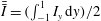 $\bar{\bar{I}}=(\int _{-1}^{1}I_{y}\,\text{d}y)/2$
, where
 $I_{y}$
is the electric current in the
 $y$
direction, i.e.
 $I_{y}=1/(2{\rm\pi}/{\it\alpha})\int _{0}^{2{\rm\pi}/{\it\alpha}}J_{y}\,\text{d}x$
. For calculation of
 $\bar{\bar{I}}$
, we substitute
 $\boldsymbol{E}=\bar{\boldsymbol{E}}+\boldsymbol{e}_{1}+\boldsymbol{e}_{2},Q=\bar{Q}+q_{1}+q_{2},\boldsymbol{U}=\bar{\boldsymbol{U}}+\boldsymbol{u}_{1}+\boldsymbol{u}_{2}$
, where the subscripts
 $_{1},_{2}$
denote first- and second-order waves. In particular, we include the second-order waves to account for the nonlinear interaction of two first-order linear waves
 $E_{w}$
–
 $E_{w}^{-1}$
. By substitution, we obtain
 $$\begin{eqnarray}\displaystyle \bar{\bar{I}} & = & \displaystyle \frac{1}{2}\int _{-1}^{1}\bar{E}\bar{Q}-\frac{1}{Fe}\frac{\partial \bar{Q}}{\partial y}+{\it\epsilon}^{2}|A_{1}|^{2}E_{t}^{\ast }E_{t}\left(\vphantom{\frac{\partial q_{20}}{\partial y}}{e_{1}}_{y}^{\ast }q_{1}+{e_{1}}_{y}q_{1}^{\ast }\right.\nonumber\\ \displaystyle & & \displaystyle \left.+\,v^{\ast }q_{1}+vq_{1}^{\ast }+\bar{E}q_{20}+e_{20}\bar{Q}+v_{20}\bar{Q}-\frac{1}{Fe}\frac{\partial q_{20}}{\partial y}\right)\,\text{d}y+O({\it\epsilon}^{4}|A_{1}|^{4}),\end{eqnarray}$$
where
 $q_{20},e_{20},v_{20}$
are base flow modifications solved in (2.22). Subsequently, after neglecting higher-order corrections, we have
 $$\begin{eqnarray}\displaystyle & \displaystyle \overline{\overline{Ne}}=\frac{\bar{\bar{I}}}{\bar{\bar{I}}_{0}}\approx 1\hspace{318.67078pt} & \displaystyle \nonumber\\ \displaystyle & \displaystyle +\,\frac{\displaystyle \int _{-1}^{1}{\it\epsilon}^{2}|A_{1}|^{2}\left({e_{1}}_{y}^{\ast }q_{1}+{e_{1}}_{y}q_{1}^{\ast }+v^{\ast }q_{1}+vq_{1}^{\ast }+\bar{E}q_{20}+e_{20}\bar{Q}+v_{20}\bar{Q}-\frac{1}{Fe}\frac{\partial q_{20}}{\partial y}\right)\,\text{d}y}{\displaystyle \int _{-1}^{1}\bar{E}\bar{Q}-\frac{1}{Fe}\frac{\partial \bar{Q}}{\partial y}\,\text{d}y}, & \displaystyle \nonumber\\ \displaystyle & & \displaystyle\end{eqnarray}$$
where equation
 $E_{t}^{\ast }E_{t}=1$
has been used since
 ${\it\mu}$
is vanishing at the critical condition. Furthermore, we can define at the critical condition, following Worraker & Richardson (Reference Worraker and Richardson1981)
 $$\begin{eqnarray}r_{el}=\lim _{{\it\epsilon}A_{1}\rightarrow 0}\frac{\overline{\overline{Ne}}-1}{{\it\epsilon}^{2}|A_{1}|^{2}}.\end{eqnarray}$$
With these assumptions made,
 $r_{el}$
can be calculated and we find at
 $C=50,M=100,Fe=10^{3},T=140.41884,{\it\alpha}=2.58674$
that
 $r_{el}=0.7383>0$
, or equivalently
 $\overline{\overline{Ne}}>1$
. It has been calculated that
 $r_{el}>0$
for a large portion of parameter space
 $M\in [5,100],Fe\in [400,10^{5}],C\in [3,100]$
. Thus, it can be said that the first-order waves and their nonlinear effect increase the value of
 $\overline{\overline{Ne}}$
(which is
 $1$
for base states).
We compare this result with the measurement made in Lacroix et al. (Reference Lacroix, Atten and Hopfinger1975). Using scaling arguments, Lacroix et al. (Reference Lacroix, Atten and Hopfinger1975) derived theoretically that
 $Ne$
is proportional to
 $T^{1/2}$
for small
 $MRe$
. Their experiments also showed that in the nonlinearly saturated phase, i.e. when steady turbulent convection is formed,
 $Ne$
in the measurement indeed varies as
 $T^{1/2}$
for small
 $T/T_{c}$
and is always greater than
 $1$
once convection sets in. When we vary
 $T$
, however, the scaling
 $\overline{\overline{Ne}}\sim T^{1/2}$
cannot be found from our data.
To properly interpret these result and comparison, the real physics in the measurements and the assumptions made in our calculation should be stated clearly. First, the definition of the electric Nusselt number is slightly different: in Lacroix et al. (Reference Lacroix, Atten and Hopfinger1975),
 $Ne$
is defined at a horizontal plane since
 $Ne$
is constant along
 $y$
in a statistically steady state as in experiments; for us, the weakly nonlinear flow is far from such a state, thus the mean Nusselt number is used. Besides, the real flow in experiments is 3-D while our calculation is 2-D. Most importantly, the measured flow corresponds to a nonlinearly saturated state of a broadband spectrum, whereas our modal expansion method is based on linear periodic waves of critical frequency and wavenumber with their low-order nonlinear effects. Therefore, it is expected that the more sophisticated scaling
 $Ne\sim T^{1/2}$
, as it describes a highly nonlinear 3-D phenomenon, cannot be reproduced by our modal expansion method (using the first-order waves). Thus, at most, only a qualitative comparison can be made between our results and the measurements. Still, from our calculation
 $\overline{\overline{Ne}}>1$
, we can conclude that the effect of first-order linear wave nonlinearly modifying the steady base flows is to help establish a higher mean electric current. To facilitate the comparison between real flow and weakly nonlinear flow, more spectral analysis of measured EHD flow in future is needed.
4.2.2 Effect of
$M$

The effect of the mobility parameter
 $M$
in the weakly nonlinear phase of hydrostatic EHD is presented as follows. In the linear phase, it has been shown and discussed that changing
 $M$
will not affect the linear stability criterion, even though the transient growth is a function of
 $M$
, see for example Zhang et al. (Reference Zhang, Martinelli, Wu, Schmid and Quadrio2015). In the weakly nonlinear phase, the effect of
 $M$
can be probed by examining the magnitudes of Landau coefficients for different
 $M$
. In Atten & Lacroix (Reference Atten and Lacroix1979), only infinite
 $M$
is considered.
The effect of
 $M$
at
 $C=50,Fe=10^{3},T=140.41884$
,
 ${\it\alpha}=2.58674$
. (a) The growth rate
 ${\it\omega}_{i}$
, (b)
 $a_{3}$
and (c)
 $a_{5}$
.

Figure 6 shows the effect of
 $M\in [5,100]$
on the hydrostatic EHD at
 $C=50,Fe=10^{3},T=140.41884,{\it\alpha}=2.58674$
in the weakly nonlinear phase. It is first checked that the growth rate
 $\text{Re}({\it\mu})={\it\omega}_{i}$
for all the
 $M$
considered here is very small
 ${\sim}O(10^{-8})$
, see panel (a), therefore close to the critical condition. As we can see in panel (b), the value of
 $a_{3}$
is increasing with increasing
 $M$
. This indicates that the subcritical feature of hydrostatic EHD flow is more pronounced as
 $M$
increases, or equivalently, the third-order nonlinear term in GLE destabilizes the flow further when
 $M$
is increased. This increasing destabilization effect is most obvious in the region of
 $M=5{-}20$
. Larger than
 $20$
, the destabilizing effect of increasing
 $M$
is approaching constant. At the higher order of nonlinearity, (c) shows that
 $a_{5}$
is decreasing with increasing
 $M$
; that is, the fifth-order nonlinear term in GLE will stabilize the flow more if
 $M$
increases. Therefore, combining these two results, it can be said that, when
 $M$
is high in hydrostatic EHD, the disturbances will grow faster due to the low-order nonlinearities in an earlier phase; whereas, when their amplitudes are large enough to trigger the higher-order nonlinearities, the disturbances will be abated more by these higher-order nonlinearities. On the other hand, when
 $M$
is small, both the destabilizing and the stabilizing effects will be more moderate.
Regarding the destabilizing effect of the leading-order nonlinearity with increasing
 $M$
as shown in (b), a similar conclusion has been drawn by Wu et al. (Reference Wu, Traoré, Pérez and Vázquez2015a
,Reference Wu, Traoré, Pérez and Zhang
b
), in which the authors studied the relationship between
 $V_{max}$
(maximum vertical velocity appearing in the flow) and
 $M$
using a DNS method. Despite the fact that their
 $T$
is above the critical
 $T_{c}$
, they reported the same trend of
 $V_{max}$
with respect to increasing
 $M$
in the SCL case, especially the trends of the asymptotic constant effect at large
 $M$
and the drastic change of
 $V_{max}$
around
 $M=10{-}20$
, see the Wu et al. (Reference Wu, Traoré, Pérez and Zhang2015b
, figure 7b). Therefore, it is cogent to say that the leading-order nonlinear term in GLE of hydrostatic EHD can predict correctly the nonlinear destabilizing effect of
 $M$
in a qualitative manner.
4.2.3 Effect of
$Fe$

The role of charge diffusion has rarely been discussed in the stability analysis of hydrostatic EHD flow. In the nonlinear stability analysis performed by Atten & Lacroix (Reference Atten and Lacroix1979), the charge diffusion is completely neglected; in the weakly nonlinear stability of ETHD flow by Worraker & Richardson (Reference Worraker and Richardson1981), they did not account for the charge diffusion effect as well.
On one hand, several authors discussed this issue and focused on the cases when the charge diffusion can be safely neglected and when not (Castellanos, Perez & Atten Reference Castellanos, Perez and Atten1989; Pérez & Castellanos Reference Pérez and Castellanos1989). For example, Castellanos et al. (Reference Castellanos, Perez and Atten1989) discussed the nonlinear motion of EHD subject to weak injection of ions in the limit of high
 $M$
with a predetermined self-similar velocity field. They concluded that, in the weak-injection limit (small
 $C$
), the parameter
 $C\sqrt{Fe}$
is indicative of the importance of charge diffusion, that is, higher
 $C\sqrt{Fe}$
indicates negligible diffusion effect and vice versa. On the other hand, few works discussed and defined clearly the effect of charge diffusion on the flow transition of EHD, except a recent example by Zhang et al. (Reference Zhang, Martinelli, Wu, Schmid and Quadrio2015), in which the authors found that the charge diffusion has a non-negligible effect on the linear stability criterion and also affects the transient dynamics of the EHD flow in the initial phase of perturbation development, even though the latter effect is small (the transient growth in hydrostatic EHD flow is generally small). To the best of our knowledge, the weakly nonlinear stability analysis of hydrostatic EHD flow taking into account the charge diffusion effect has not been documented.
In figure 7, we show the effect of
 $Fe$
on the linear stability criterion
 $T_{c}$
in (a), the value of
 $a_{3}$
in (b) and
 $a_{5}$
in (c). The range of
 $Fe$
considered is
 $[400,10^{5}]$
, outside of which significant relative error results in terms of the dispersion relation, so those results are probably contaminated by numerical errors; nevertheless, the considered values of
 $Fe$
are representative, covering a large enough range to investigate the effect of charge diffusion on the flow dynamics. And the physical value of
 $Fe$
lies in
 $[10^{3},10^{4}]$
. As the critical condition around the first bifurcation is investigated here, the critical
 $T_{c}$
changes as
 $Fe$
increases, presented in (a). Higher
 $Fe$
(smaller charge diffusion effect) leads to greater
 $T_{c}$
, thus a more stable flow. In (b), we see that when the charge diffusion effect is significant (smaller
 $Fe$
), the value of
 $a_{3}$
decreases, indicating that the subcritical characteristics of EHD flow becomes smaller. In (c), it shows that the value of
 $a_{5}$
is increasing when
 $Fe$
decreases. Thus, stronger charge diffusion stabilizes the flow less at the fifth-order nonlinearity.
From these results, therefore, a conclusion can be drawn that the charge diffusion destabilizes the linearized EHD flow, but stabilizes the flow in an early phase of the nonlinear development of the disturbance (related to
 $a_{3}$
). This dual effect of charge diffusion in the weakly nonlinear phase is consistent with the results obtained by the DNS method in the earlier works, for example, Castellanos et al. (Reference Castellanos, Perez and Atten1989), in which they have shown a similar trend in that when the charge diffusion effect is intensified (smaller
 $Fe$
), the linear stability criterion decreases and the nonlinear stability criterion (
 $T_{f}$
) increases, resulting in a less subcritical flow. This decrease of the subcritical feature with decreasing
 $Fe$
can be interpreted together with the effect of charge diffusion on the hysteresis loop (Castellanos, Atten & Perez Reference Castellanos, Atten and Perez1987). Smaller
 $T_{f}{-}T_{c}$
corresponds to a smaller hysteresis loop and a smaller area of charge void region as pointed out by Pérez & Castellanos (Reference Pérez and Castellanos1989). In their work, the authors also discussed that the ‘separatrix’ delimiting the charge existing region from the charge void region becomes blurred when the charge diffusion effect is taken into account (this separatrix would be discontinuous if
 $Fe\rightarrow \infty$
).
The effect of
 $Fe$
at
 $C=12.5,M=100$
at the critical condition. (a) The critical
 $T_{c}$
, (b)
 $a_{3}$
and (c)
 $a_{5}$
.

4.2.4 Effect of C
We also investigate the effect of
 $C$
, the injection level, on the nonlinear subcritical bifurcation of hydrostatic EHD flow in the weakly nonlinear phase. Note that, as explained in the problem formulation section, there is a factor of four between our
 $C$
, defined with respect to the half-channel distance, and the
 $C$
defined according to the full-channel distance, which is the usual convention in the EHD community. Thus the interpretation of the quantitative results relevant to
 $C$
should be exercised with this difference kept in mind.
In figure 8(a), the critical value of
 $T_{c}$
solved from the linear stability problem is shown to decrease with increasing
 $C$
. In the linear phase of EHD subject to strong injection level, higher
 $C$
will give rise to a more destabilized flow in both modal and non-modal stability analyses (Zhang et al.
Reference Zhang, Martinelli, Wu, Schmid and Quadrio2015), although the latter effect is not significant. In (b), it describes how the value of
 $a_{3}$
changes with different values of
 $C$
at the critical condition; that is, increasing
 $C$
reduces the destabilizing effect of the third-order nonlinearity in the hydrostatic EHD flow. At the fifth-order nonlinearity, the stabilizing effect is also decreasing at higher
 $C$
. Therefore, the effect of
 $C$
on the nonlinearity is in the opposite sense to that of increasing
 $M$
or
 $Fe$
, which is clear by comparing figure 8 with figure 6 or 7.
The effect of
 $C$
at
 $Fe=10^{3},M=100$
at the critical condition. (a) The critical
 $T_{c}$
, (b)
 $a_{3}$
and (c)
 $a_{5}$
.

Modification of base electric field in hydrostatic EHD.
 $Fe=10^{3},M=100$
. Blue solid lines:
 $C=50,T=140.41884,{\it\alpha}=2.58674$
. Red dashed lines:
 $C=10,T=144.48175,{\it\alpha}=2.57780$
. Black lines with dots:
 $C=3,T=152.62120,{\it\alpha}=2.5575$
. (a) Modification of base potential
 $\tilde{{\it\varphi}}_{20}^{\prime }$
, (b) modification of base charge distribution
 $\tilde{{\it\varphi}}_{20}^{\prime \prime }/(-C)$
.

4.2.5 Modification of base electric field
The term
 $\tilde{{\it\gamma}}_{20}=(\tilde{{\it\psi}}_{20},\tilde{{\it\varphi}}_{20})^{\text{T}}$
represents the leading-order modification of the base flow state by the nonlinear interaction between the first-order linear waves
 $E_{w}$
and
 $E_{w}^{-1}$
. The base flow modification
 $\tilde{{\it\psi}}_{20}^{\prime }$
(note the relation that
 $u={\it\psi}^{\prime }$
) has been discussed in the context of, for example, Poiseuille flow (Plaut et al.
Reference Plaut, Lebranchu, Simitev and Busse2008) and non-Newtonian channel flow (Chekila et al.
Reference Chekila, Nouar, Plaut and Nemdili2011). For hydrostatic EHD flow, the base flow modification
 $\tilde{{\it\psi}}_{20}^{\prime }=0$
as
 $\bar{U}=0$
, thus we will only discuss it below in the cross-flow case.
Here, we present the base potential modification
 $\tilde{{\it\varphi}}_{20}$
due to the
 $E_{w}{-}E_{w}^{-1}$
wave interaction. In figure 9(a), we see that the general modification of the base potential is the decrease of its value around the centreline. When the charge injection level increases in the SCL regime, this decrease is slightly amplified. In (b), it shows the effect of nonlinear modification on the base charge distribution
 $\tilde{{\it\varphi}}_{20}^{\prime \prime }/(-C)$
(see (2.1d
)). The result indicates that the charge distribution at the channel centreline decreases, but increases dramatically close to the injector (
 $y=1$
). The former result is consistent with the formation of charge void region in the finite-amplitude convection motion usually obtained in the DNS results, in which there is almost zero charge density around the centre of the channel, see, for example, Wu et al. (Reference Wu, Traoré, Vázquez and Pérez2013). For the latter result, it is hard to connect it directly with the DNS outcome. However, as the increase of charged ions in this region is quite steep, further nonlinearity might be triggered and should be taken into account.
4.2.6 Nonlinear terms
In order to probe which terms are the most responsible for the subcritical bifurcation of hydrostatic EHD, the contributions of different parts to the resultant value of
 $a_{3}$
are examined. We analyse the nonlinear effects by decomposing
 $a_{3}$
as
 $$\begin{eqnarray}a_{3}=\frac{\langle \unicode[STIX]{x1D649}_{3_{1}}^{\circ },\tilde{{\it\psi}_{1}}^{\dagger }\rangle _{s}+\langle \unicode[STIX]{x1D649}_{3_{2}}^{\circ },\tilde{{\it\varphi}_{1}}^{\dagger }\rangle _{s}}{\langle \unicode[STIX]{x1D648}_{0}\tilde{{\it\gamma}_{1}},\tilde{{\it\gamma}_{1}}^{\dagger }\rangle _{s}}=\{\unicode[STIX]{x1D649}_{3_{1}}^{\circ }\}+\{\unicode[STIX]{x1D649}_{3_{2}}^{\circ }\},\end{eqnarray}$$
where we have used
 $\{\dot{~}\}$
to denote
 $\langle \dot{~},\tilde{{\it\psi}_{1}}^{\dagger }\rangle _{s}/\langle \unicode[STIX]{x1D648}_{0}\tilde{{\it\gamma}_{1}},\tilde{{\it\gamma}_{1}}^{\dagger }\rangle _{s}$
or
 $\langle \dot{~},\tilde{{\it\varphi}_{1}}^{\dagger }\rangle _{s}/\langle \unicode[STIX]{x1D648}_{0}\tilde{{\it\gamma}_{1}},\tilde{{\it\gamma}_{1}}^{\dagger }\rangle _{s}$
. The terms of
 $\unicode[STIX]{x1D649}_{3}=(\unicode[STIX]{x1D649}_{3_{1}},\unicode[STIX]{x1D649}_{3_{2}})^{\text{T}}$
are the nonlinear terms of the order of
 ${\it\epsilon}^{3}$
in (2.3b
) and (2.3c
), respectively. Their expressions are listed below
 $$\begin{eqnarray}\displaystyle \unicode[STIX]{x1D649}_{3_{1}} & = & \displaystyle -\hspace{-2.0pt}\left[\frac{\partial {\it\psi}_{1}}{\partial y}\left(2\frac{\partial ^{2}}{\partial x_{0}^{2}}\frac{\partial {\it\psi}_{1}}{\partial x_{1}}+\frac{\partial }{\partial x_{1}}{\rm\nabla}_{0}^{2}{\it\psi}_{1}+\frac{\partial }{\partial x_{0}}{\rm\nabla}_{0}^{2}{\it\psi}_{2}\right)+\frac{\partial {\it\psi}_{2}}{\partial y}\frac{\partial }{\partial x_{0}}{\rm\nabla}_{0}^{2}{\it\psi}_{1}\right.\nonumber\\ \displaystyle & & \displaystyle -\,\underbrace{\displaystyle \left.\left[\frac{\partial {\it\psi}_{1}}{\partial x_{0}}\left(2\frac{\partial }{\partial y}\frac{\partial }{\partial x_{0}}\frac{\partial {\it\psi}_{1}}{\partial x_{1}}+\frac{\partial }{\partial y}{\rm\nabla}_{0}^{2}{\it\psi}_{2}\right)+\left(\frac{\partial {\it\psi}_{1}}{\partial x_{1}}+\frac{\partial {\it\psi}_{2}}{\partial x_{0}}\right)\frac{\partial }{\partial y}{\rm\nabla}_{0}^{2}{\it\psi}_{1}\right]\right]}_{\unicode[STIX]{x1D649}_{3_{1A}}}\nonumber\\ \displaystyle & & \displaystyle -\,M^{2}\left[\frac{\partial {\it\varphi}_{1}}{\partial y}\left(2\frac{\partial ^{2}}{\partial x_{0}^{2}}\frac{\partial {\it\varphi}_{1}}{\partial x_{1}}+\frac{\partial }{\partial x_{1}}{\rm\nabla}_{0}^{2}{\it\varphi}_{1}+\frac{\partial }{\partial x_{0}}{\rm\nabla}_{0}^{2}{\it\varphi}_{2}\right)+\frac{\partial {\it\varphi}_{2}}{\partial y}\frac{\partial }{\partial x_{0}}{\rm\nabla}_{0}^{2}{\it\varphi}_{1}\right.\nonumber\\ \displaystyle & & \displaystyle -\,\underbrace{\displaystyle \left.\left[\frac{\partial {\it\varphi}_{1}}{\partial x_{0}}\left(2\frac{\partial }{\partial y}\frac{\partial }{\partial x_{0}}\frac{\partial {\it\varphi}_{1}}{\partial x_{1}}+\frac{\partial }{\partial y}{\rm\nabla}_{0}^{2}{\it\varphi}_{2}\right)f+\left(\frac{\partial {\it\varphi}_{1}}{\partial x_{1}}+\frac{\partial {\it\varphi}_{2}}{\partial x_{0}}\right)\frac{\partial }{\partial y}{\rm\nabla}_{0}^{2}{\it\varphi}_{1}\right]\right]}_{\unicode[STIX]{x1D649}_{3_{1B}}},\end{eqnarray}$$
 $$\begin{eqnarray}\displaystyle \unicode[STIX]{x1D649}_{3_{2}} & = & \displaystyle \underbrace{\displaystyle \left(\frac{\partial {\it\varphi}_{1}}{\partial x_{0}}-\frac{\partial {\it\psi}_{1}}{\partial y}\right)\left(2\frac{\partial ^{2}}{\partial x_{0}^{2}}\frac{\partial {\it\varphi}_{1}}{\partial x_{1}}+\frac{\partial }{\partial x_{1}}{\rm\nabla}_{0}^{2}{\it\varphi}_{1}+\frac{\partial }{\partial x_{0}}{\rm\nabla}_{0}^{2}{\it\varphi}_{2}\right)}_{\unicode[STIX]{x1D649}_{3_{2A}}}\nonumber\\ \displaystyle & & \displaystyle +\,\underbrace{\displaystyle \left(\frac{\partial {\it\varphi}_{1}}{\partial x_{1}}+\frac{\partial {\it\varphi}_{2}}{\partial x_{0}}-\frac{\partial {\it\psi}_{2}}{\partial y}\right)\frac{\partial }{\partial x_{0}}{\rm\nabla}_{0}^{2}{\it\varphi}_{1}}_{\unicode[STIX]{x1D649}_{3_{2B}}}+\underbrace{\displaystyle \left(\frac{\partial {\it\varphi}_{1}}{\partial y}+\frac{\partial {\it\psi}_{1}}{\partial x_{0}}\right)\left(\frac{\partial }{\partial y}{\rm\nabla}_{0}^{2}{\it\varphi}_{2}+2\frac{\partial }{\partial y}\frac{\partial }{\partial x_{0}}\frac{\partial {\it\varphi}_{1}}{\partial x_{1}}\right)}_{\unicode[STIX]{x1D649}_{3_{2C}}}\nonumber\\ \displaystyle & & \displaystyle +\,\underbrace{\left(\frac{\partial {\it\varphi}_{2}}{\partial y}+\frac{\partial {\it\psi}_{1}}{\partial x_{1}}+\frac{\partial {\it\psi}_{2}}{\partial x_{0}}\right)\frac{\partial }{\partial y}{\rm\nabla}_{0}^{2}{\it\varphi}_{1}}_{\unicode[STIX]{x1D649}_{3_{2D}}}+\underbrace{2\left(2\frac{\partial ^{2}{\it\varphi}_{1}}{\partial x_{0}\partial x_{1}}+{\rm\nabla}_{0}^{2}{\it\varphi}_{2}\right){\rm\nabla}_{0}^{2}{\it\varphi}_{1}}_{\unicode[STIX]{x1D649}_{3_{2E}}},\end{eqnarray}$$
 ${\rm\nabla}_{0}^{2}=(\partial ^{2}/\partial x_{0}^{2})+(\partial ^{2}/\partial y^{2})$
.
The respective values of these two terms are calculated at the critical condition
 $C=50,M=100,Fe=10^{3},T=140.41884,{\it\alpha}=2.58674$
with the value of
 $a_{3}$
shown in table 2, and we obtain
 $$\begin{eqnarray}\{\unicode[STIX]{x1D649}_{3_{1}}^{\circ }\}=0.09158,\quad \{\unicode[STIX]{x1D649}_{3_{2}}^{\circ }\}=17.09803.\end{eqnarray}$$
This indicates that the subcritical nature of the hydrostatic EHD flow is mainly related to the nonlinear terms in the governing equation for
 ${\it\varphi}$
, the perturbed potential. We can dig further by computing the respective terms
 $\unicode[STIX]{x1D649}_{3_{2A}}^{\circ },\unicode[STIX]{x1D649}_{3_{2B}}^{\circ },\unicode[STIX]{x1D649}_{3_{2C}}^{\circ },\unicode[STIX]{x1D649}_{3_{2D}}^{\circ },\unicode[STIX]{x1D649}_{3_{2E}}^{\circ }$
of
 $\unicode[STIX]{x1D649}_{3_{2}}^{\circ }$
. Our calculation yields
 $$\begin{eqnarray}\{\unicode[STIX]{x1D649}_{3_{2A}}^{\circ }\}=-0.35022,\end{eqnarray}$$
 $$\begin{eqnarray}\{\unicode[STIX]{x1D649}_{3_{2B}}^{\circ }\}=0.53866,\quad \{\unicode[STIX]{x1D649}_{3_{2C}}^{\circ }\}=14.66630,\end{eqnarray}$$
 $$\begin{eqnarray}\{\unicode[STIX]{x1D649}_{3_{2D}}^{\circ }\}=-1.52122,\quad \{\unicode[STIX]{x1D649}_{3_{2E}}^{\circ }\}=3.76452.\end{eqnarray}$$
From the results above, we see immediately that the terms in
 $\unicode[STIX]{x1D649}_{3_{2C}}^{\circ }$
give the maximum destabilizing effect. From (4.9b
),
 $\unicode[STIX]{x1D649}_{3_{2C}}^{\circ }$
is further decomposed as
 $$\begin{eqnarray}\displaystyle \left\{\frac{\partial {\it\varphi}_{1}}{\partial y}\left(\frac{\partial }{\partial y}{\rm\nabla}_{0}^{2}{\it\varphi}_{2}+2\frac{\partial }{\partial y}\frac{\partial }{\partial x_{0}}\frac{\partial {\it\varphi}_{1}}{\partial x_{1}}\right)\right\} & = & \displaystyle -1.19226,\end{eqnarray}$$
 $$\begin{eqnarray}\displaystyle \left\{\frac{\partial {\it\psi}_{1}}{\partial x_{0}}\left(\frac{\partial }{\partial y}{\rm\nabla}_{0}^{2}{\it\varphi}_{2}+2\frac{\partial }{\partial y}\frac{\partial }{\partial x_{0}}\frac{\partial {\it\varphi}_{1}}{\partial x_{1}}\right)\right\} & = & \displaystyle 15.85856.\end{eqnarray}$$
 $(\partial {\it\psi}_{1}/\partial x_{0})$
and the second-order
 $(\partial /\partial y){\rm\nabla}_{0}^{2}{\it\varphi}_{2}+2(\partial /\partial y)(\partial /\partial x_{0})(\partial {\it\varphi}_{1}/\partial x_{1})$
generates the most significant destabilizing effect, helping to form the subcritical bifurcation of hydrostatic EHD.
As these results show that the terms involving the streamfunction perturbation
 ${\it\psi}_{1}$
(see (4.12b
)) are predominating in the determination of the nonlinear destabilizing effect in hydrostatic EHD subject to strong injection (
 $C=50$
), this seems to indicate that a dynamic and accurate model for the velocity field should be provided for a rigorous and formal attempt of conducting weakly nonlinear stability analysis of EHD flow, at least of the order of
 ${\it\epsilon}^{3}$
. In fact, when assuming that the velocity field be approximated by a predetermined self-similar roll structure in several past works, for example, Atten & Lacroix (Reference Atten and Lacroix1979), one loses such a dynamic description of the velocity field and therefore its dynamic interaction with the electric field. This point of view has also been noted in Traoré & Wu (Reference Traoré and Wu2013) in the case of weak injection. Nevertheless, these results should not be interpreted to criticize the velocity-predetermined method. In fact, it is held that the merit of the velocity-predetermined method should not be denied owing to its success in predicting and revealing, for example, the subcritical bifurcation of hydrostatic EHD, for an informal and quick check of the nonlinear effect.
4.3 EHD with cross-flow
The linear stability of EHD with cross-flow has been studied in Atten & Honda (Reference Atten and Honda1982), Castellanos & Agrait (Reference Castellanos and Agrait1992) and more recently Zhang et al. (Reference Zhang, Martinelli, Wu, Schmid and Quadrio2015). It is interesting to see how the 2-D channel flow is influenced by the electric field in the weakly nonlinear phase, which has not been reported in the literature. In this section, we first show the base flow modification in the EHD flow with low-
 $Re$
cross-flow and then we present the various results for the high-
 $Re$
EHD-Poiseuille flow.
4.3.1 Low
$Re$
cross-flow: base flow modification

We focus on how the base flow is modified by the electric field in this case. In hydrostatic EHD, as
 $\bar{U}=0$
, the modification of base flow is also zero, whereas for low-
 $Re$
EHD,
 $\bar{U}\neq 0$
, and thus the nonlinearity will modify the base flow. The base flow modification
 $\tilde{{\it\psi}}_{20}^{\prime }$
is shown in figure 10 for two small different
 $Re$
in (a) and for three different
 $C$
in (b) at the critical condition. From these results, the general modifications of the base flow by the electric field are that the flow is decelerated in the region from the injector electrode (
 $y=1$
) to around the channel centreline, slightly decelerated close to the collector and between these two regions the flow is accelerated. In (a), the effect of the flow rate is examined (base flow of the red curve is
 $\bar{U}=1-y^{2}$
, whereas, that of the blue curve with circles is
 $\bar{U}=(1-y^{2})/2$
); when the
 $Re$
is doubled, the flow modification effect is also amplified. In (b), the effect of the electric field is investigated; with increasing
 $C$
, the base flow modification is strengthened, but since we are in the strong injection limit, the difference among
 $C=3,10$
and
 $50$
is not so exaggerated.
4.3.2 High
$Re$
cross-flow: effect of
$T$


For EHD with high-
 $Re$
cross-flow, we concentrate on the effect of
 $T$
primarily. When
 $Re\in [10^{3},10^{4}]$
and
 $T\in [10^{2},10^{3}]$
,
 $M=\sqrt{T/Re}$
takes the value of
 $[10^{-2},1]$
, implying that the working fluid is a gas and that the weakly nonlinear effect is examined pertaining to the 2-D Tollmien–Schlichting wave.
Modification of base flow
 $\tilde{{\it\psi}}_{20}^{\prime }$
(real part) for EHD with low-
 $Re$
cross-flow. (a)
 $C=10,M=100,Fe=10^{3}$
. Blue line with circles:
 $T=143.5852,{\it\alpha}=2.5628,Re=T/(2M^{2})=0.0071$
. Red solid line:
 $T=142.0188,{\it\alpha}=2.5015,Re=T/M^{2}=0.0142$
; (b)
 $M=100,Fe=10^{3}$
. Blue solid line:
 $C=50,T=138.4069,{\it\alpha}=2.5108,Re=T/M^{2}=0.0138$
. Red dashed line:
 $C=10,T=142.0188,{\it\alpha}=2.5015,Re=T/M^{2}=0.0142$
. Black line with circles:
 $C=3,T=150.3564,{\it\alpha}=2.4765,Re=T/M^{2}=0.0150$
.

In figure 11, we present the change of the Landau coefficients when the electric field is imposed at
 $C=50,Fe=10^{3},M=\sqrt{T/Re}$
compared to conventional channel flow (
 $T\rightarrow 0$
). The constraint of
 $M=\sqrt{T/Re}$
is to enforce the constant flow rate, see Zhang et al. (Reference Zhang, Martinelli, Wu, Schmid and Quadrio2015). Since now there is a cross-flow, the Landau coefficients are complex (travelling wave solutions); we, nevertheless only show the real part in the results below. As we investigate the first bifurcation of the flows around the critical condition,
 $Re_{c}$
and
 ${\it\alpha}$
are changing for increasing
 $T$
; specifically, the critical
 $Re_{c}$
as a function of
 $T$
, shown in (a), decreases when
 $T$
increases, indicating that the flow inertia is smaller when the EHD-Poiseuille flow of the stronger electric effect encounters the first bifurcation, which is consistent with the results obtained in Zhang et al. (Reference Zhang, Martinelli, Wu, Schmid and Quadrio2015) where we have shown that EHD-Poiseuille flow may become more unstable in terms of modal and non-modal linear stability theory compared to canonical channel flow. In (b), with the current probing values of
 $T$
, we can see that with higher electric potential difference imposed, the subcritical characteristics of the EHD-Poiseuille flow becomes more pronounced due to the nonlinear effect, as the real part of
 $a_{3}$
is increasing with higher
 $T$
. The change of the real part of
 $a_{5}$
is shown in (c), according to which we can say that the stabilizing effect of the fifth-order nonlinearity is increasing as
 $T$
increases.
The effect of
 $T$
at the critical condition with
 $C=50,Fe=10^{3},M=\sqrt{T/Re}$
. (a)
 $Re_{c}$
as a function of
 $T$
, (b) the real part of
 $a_{3}$
as a function of
 $T$
and (c) the real part of
 $a_{5}$
as a function of
 $T$
.
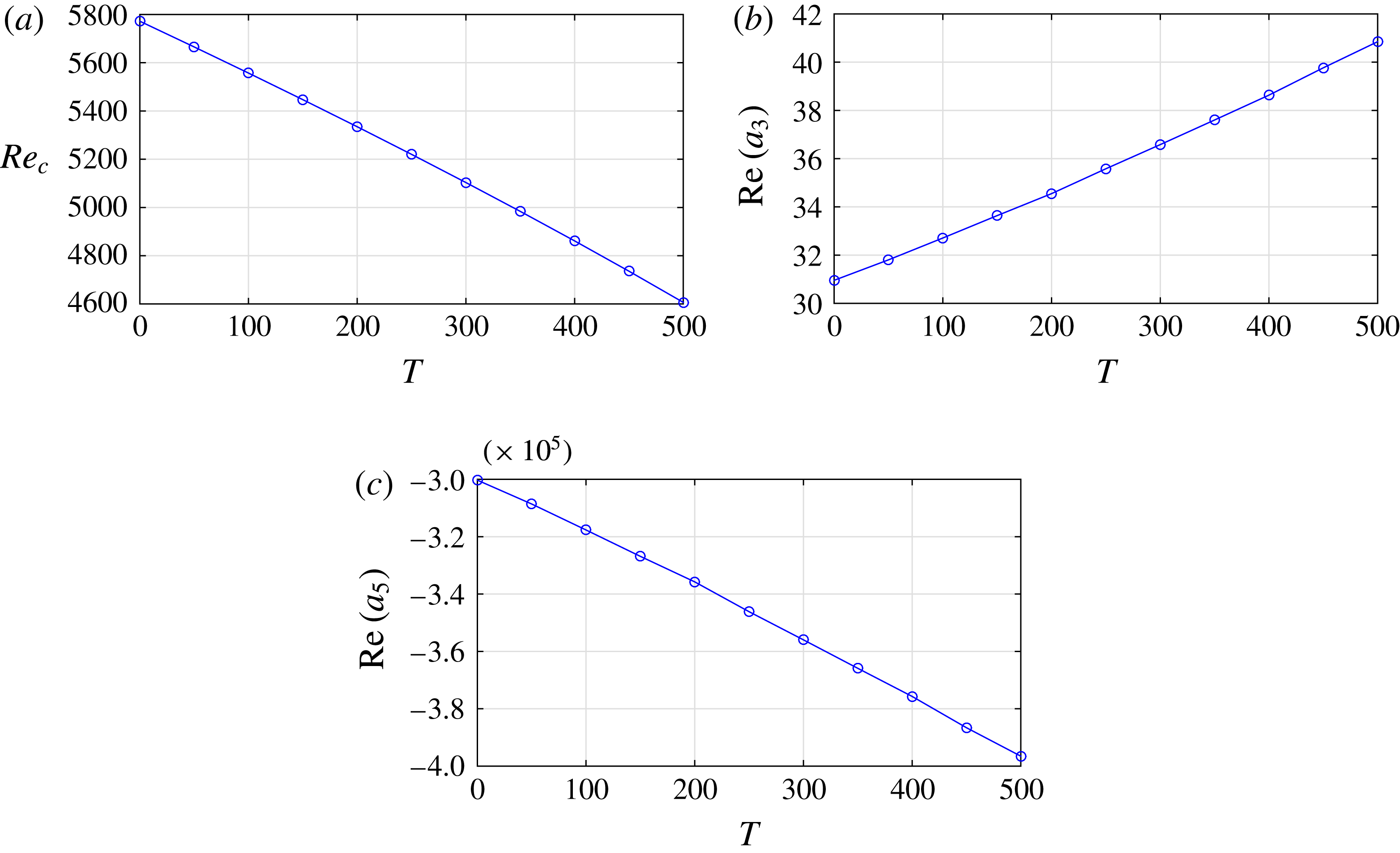
Base flow modification at the critical condition. (a) Real part of
 $\tilde{{\it\psi}}_{20}^{\prime }$
. Blue solid line: canonical Poiseuille flow at
 $Re=5772.2218,{\it\alpha}=1.0205474$
; red dashed line: EHD-Poiseuille flow at
 $T=100,Re=5557.2000,{\it\alpha}=1.0244,C=50,Fe=10^{3},M=\sqrt{T/Re}=0.13414$
; black lines with pluses:
 $T=500,Re=4606.5458,{\it\alpha}=1.0443,C=50,Fe=10^{3},M=\sqrt{T/Re}=0.32946$
. (b) The difference between base flow modifications of EHD-Poiseuille flow (real part of
 $\tilde{{\it\psi}}_{20,EHD\text{-}P}^{\prime }$
) and canonical Poiseuille flow (real part of
 $\tilde{{\it\psi}}_{20,Poiseuille}^{\prime }$
). Red dashed line:
 $T=100$
, black line with pluses:
 $T=500$
with the other parameters the same as in (a).

4.3.3 High
$Re$
cross-flow: base flow modification

The base flow modification
 $\tilde{{\it\psi}}_{20}^{\prime }$
is presented in figure 12 for
 $T=0,100,500$
in the high-
 $Re$
cross-flow case. Our result of the conventional Poiseuille flow (blue solid curve in figure 12(a)) is in very good accordance with that shown in Plaut et al. (Reference Plaut, Lebranchu, Simitev and Busse2008) for Poiseuille flow with fixed flow rate. We see that
 $\tilde{{\it\psi}}_{20}^{\prime }$
for Poiseuille flow is symmetric with respect to the channel centreline and that the nonlinearity mildly accelerates the laminar flow near to the walls, drastically accelerates the flow around the centre of the channel and decelerates the flow in between around
 $y=\pm 0.8$
.
With the imposed electric field, the distortion of the base flow due to the nonlinearity is in general similar to that in canonical channel flow, as it is in the inertia-dominated regime (high
 $Re$
), but clearly reflects the influence from the electric field. For
 $T=100$
, the parameters at the critical condition are
 $Re_{c}=5557.2000,{\it\alpha}=1.0244,C=50,Fe=10^{3},M=\sqrt{T/Re}=0.13414$
and for
 $T=500$
, the parameters are
 $Re_{c}=4606.5458,{\it\alpha}=1.0443,M=\sqrt{T/Re}=0.32946$
and
 $C,Fe$
are the same as
 $T=100$
. It can be seen in (a) that with the electric field imposed, near the injector
 $y=1$
and the receptor
 $y=-1$
, the flow is less accelerated than the plane channel flow; this effect is stronger near the injector. When
 $y$
is around
 $0.8$
, the Poiseuille flow is decelerated most and the electric field reinforces this effect, while near
 $y=-0.8$
, the deceleration is mitigated owing to the presence of the electric field. Furthermore, around the channel centre, the EHD-Poiseuille flow is accelerated further compared to the Poiseuille flow with the highest value of
 $\tilde{{\it\psi}}_{20}$
biased to the receptor. Besides, it is interesting to show the difference between
 $\tilde{{\it\psi}}_{20}$
in the EHD-Poiseuille system and
 $\tilde{{\it\psi}}_{20}$
in the Poiseuille flow, as in (b). Clearly, the general shape of the difference in the base flow modifications is similar to those shown in figure 10 in which the base flow modification almost solely results from the electric effect (
 $Re$
is very small). But, we can also see some influence from the cross-flow in the modification as the profile becomes more wavy compared to that in figure 10.
4.3.4 High
$Re$
cross-flow: nonlinear terms

To study which part in the nonlinear terms contributes most to the subcritical characteristics of the EHD-Poiseuille flow, we show the values of
 ${\it\epsilon}^{3}$
nonlinear terms in (2.4). The terms are listed below
 $$\begin{eqnarray}-\hspace{-2.0pt}\left(\frac{\partial {\it\psi}}{\partial y}\frac{\partial {\rm\nabla}^{2}{\it\psi}}{\partial x}-\frac{\partial {\it\psi}}{\partial x}\frac{\partial {\rm\nabla}^{2}{\it\psi}}{\partial y}\right)\quad \text{and}\quad -\hspace{-2.0pt}M^{2}\left(\frac{\partial {\it\varphi}}{\partial y}\frac{\partial {\rm\nabla}^{2}{\it\varphi}}{\partial x}-\frac{\partial {\it\varphi}}{\partial x}\frac{\partial {\rm\nabla}^{2}{\it\varphi}}{\partial y}\right).\end{eqnarray}$$
The
 ${\it\epsilon}$
expansion of these two terms can also be found in (4.9a
) denoted as
 $\unicode[STIX]{x1D649}_{3_{1A}}$
and
 $\unicode[STIX]{x1D649}_{3_{1B}}$
, representing the nonlinearity due to the pure hydrodynamic part and the electric part, respectively. Obviously, when
 $T=0$
, we have
 $\unicode[STIX]{x1D649}_{3_{1B}}=0$
and all the nonlinear destabilizing effect of
 $a_{3}$
(positive
 $\text{Re}(a_{3})$
) comes from the hydrodynamic part. When
 $T=100,Re=5557.2000,{\it\alpha}=1.0244$
, we obtain the values below (the real part)
 $$\begin{eqnarray}\displaystyle \text{Re}(\{\unicode[STIX]{x1D649}_{3_{1}}^{\circ }\}) & = & \displaystyle 32.71339,\end{eqnarray}$$
 $$\begin{eqnarray}\displaystyle \text{Re}(\{\unicode[STIX]{x1D649}_{3_{1A}}^{\circ }\}) & = & \displaystyle 32.71508,\end{eqnarray}$$
 $$\begin{eqnarray}\displaystyle \text{Re}(\{\unicode[STIX]{x1D649}_{3_{1B}}^{\circ }\}) & = & \displaystyle -0.00169,\end{eqnarray}$$
 $$\begin{eqnarray}\displaystyle \text{Re}(\{\unicode[STIX]{x1D649}_{3_{2}}^{\circ }\}) & = & \displaystyle -0.00286.\end{eqnarray}$$
 $Re$
is high), it appears that the electric effect does not destabilize the flow directly, since the real parts of
 $\unicode[STIX]{x1D649}_{3_{1B}}$
and
 $\unicode[STIX]{x1D649}_{3_{2}}$
are negligible or, in fact, slightly negative. This indirect effect of the electric field on the stability or instability of EHD-Poiseuille has also been seen in the non-modal linear stability results where the transient energy amplification attributed to the electric field is minor, see the appendix in Zhang et al. (Reference Zhang, Martinelli, Wu, Schmid and Quadrio2015). On the other hand, we see that the real part of
 $\unicode[STIX]{x1D649}_{3_{1A}}$
is higher than that of conventional channel flow (the value is
 $30.95616$
at
 $Re=5772.2218,{\it\alpha}=1.0205474$
), indicating that the subcritical feature of the EHD-Poiseuille flow is stronger than that of canonical channel flow at the linear criticality. Note that, in Sen & Venkateswarlu (Reference Sen and Venkateswarlu1983), it is calculated that
 $\text{Re}(a_{3})=28.88$
at
 $Re=5774,{\it\alpha}=1.02$
while
 $\text{Re}(a_{3})=27.31$
at
 $Re=5500,{\it\alpha}=1.02$
for Poiseuille flow of fixed pressure gradient using the Reynolds & Potter method (Reynolds & Potter Reference Reynolds and Potter1967); this indicates that, for canonical Poiseuille flow,
 $\text{Re}(a_{3})$
becomes smaller when
 $Re$
decreases. From the results above, it is clear that the intensified subcritical characteristics of EHD-Poiseuille flow result from the modified flow field of channel flow owing to the imposed electric field, rather than directly from the electric effect.
5 Discussion and conclusions
In this paper, we applied multiple-scale analysis to investigate in detail the weakly nonlinear stability of 2-D EHD, with and without cross-flow, in the limit of strong charge injection. This work follows closely our previous attempt (Zhang et al.
Reference Zhang, Martinelli, Wu, Schmid and Quadrio2015) to understand the flow transition mechanism in EHD using the modal and non-modal linear stability tools. In the present work, we studied the effects of different non-dimensional parameters
 $M,Fe,C,T$
on the Landau coefficients in the quintic Ginzburg–Landau equation and also investigated the base state modifications due to the electric field. We additionally examined which nonlinear terms are the most relevant to the subcritical bifurcation of EHD flow.
5.1 Hydrostatic EHD flow
In the results of hydrostatic EHD flow, its subcritical feature of bifurcation is confirmed by the positive value of
 $a_{3}$
in GLE and negative
 $a_{5}$
, stabilizing the flow. In the parametric study, we find that varying
 $M$
does not change the linear criterion
 $T_{c}$
, however, in the nonlinear phase, greater
 $M$
destabilizes the flow more compared to smaller
 $M$
, when the perturbation amplitude is small and stabilizes the flow more when the disturbance amplitude is large enough. This strengthened subcritical feature, owing to increasing
 $M$
, is consistent with the results obtained in Wu et al. (Reference Wu, Traoré, Pérez and Vázquez2015a
,Reference Wu, Traoré, Pérez and Zhang
b
) using the DNS method.
The charge diffusion effect has long been neglected due to its small value, but we find that the disturbance wave in the weakly nonlinear phase of EHD is significantly influenced by
 $Fe$
, the reciprocal of the non-dimensionalized charge diffusion coefficient. For example, our calculation in figure 7 shows that
 $a_{3}$
decreases from
 $24.74191$
to
 $17.80560$
when
 $Fe$
changes from
 $10^{5}$
to
 $10^{3}$
, the latter lying in the range of the physical values of
 $Fe$
for real fluids (Pérez & Castellanos Reference Pérez and Castellanos1989). Therefore, the effect of charge diffusion is indeed non-negligible and even important for the flow dynamics of weakly nonlinear EHD. This leads us to the suggestion that charge diffusion not be excluded in flow modelling. Besides, as charge diffusion was often neglected in the previous works, it can be deduced that the true nonlinear criterion
 $T_{f}$
should be higher than those values computed in the previous literature excluding the modelling of charge diffusion, as the
 ${\it\epsilon}^{3}$
-order nonlinear destabilizing effect should be smaller if we take into account charge diffusion. Note that this is only a reasonable deduction of our results of the charge diffusion effect, performed around
 $T_{c}$
, to
 $T_{f}$
, probably outside of the validity range of the weakly nonlinear stability analysis near
 $T_{c}$
; nevertheless, this deduction is consistent with the results in Castellanos et al. (Reference Castellanos, Perez and Atten1989).
Besides, various effects of first-order linear waves are discussed in the linear and weakly nonlinear phases. We calculate the mean Nusselt number
 $\overline{\overline{Ne}}$
based on the base states plus the first-order linear waves and their nonlinear effects. The results compare favourably to measurements in a qualitative manner. Its value greater than
 $1$
is consistent with the measured
 $Ne$
in Lacroix et al. (Reference Lacroix, Atten and Hopfinger1975) when convection sets in, indicating that one of the effects of first-order linear waves is to help establish a higher electric current. However, the more sophisticated scaling
 $Ne\sim T^{1/2}$
cannot be reproduced from our results because of the limitation of the approach to represent fully nonlinear phenomena. In addition, we also show how the base electric field can be modified by the interaction between first-order linear waves. The base potential profile around the channel centreline decreases most. The base charge density distribution decreases at the channel centre as well, but increases dramatically near the injector electrode. Another piece of information from our results is that the accurate characterization of the subcritical feature of hydrostatic EHD also involves the first-order wave of streamfunction disturbance (hydrodynamic part) and thus, the assumption of predetermined self-similar velocity field should be avoided for any serious attempt of nonlinear analysis in the SCL regime. We hope that these results are interesting from the point of view of flow physics and flow transition to turbulence mechanism for hydrostatic EHD flow.
5.2 EHD-Poiseuille flow
With the presence of cross-flow, we see that the base flow will be modified by the electric field and the modification is generally similar for low- or high-
 $Re$
cross-flow. The base flow in the region from the injector to the channel centreline is greatly decelerated, the flow close to the collector is decelerated very slightly and in between, the flow is accelerated. In high-
 $Re$
flow, we are in the range of high inertia, thus the modification of the EHD base flow is similar to that in canonical channel flow. Additionally, we also consider the effect of
 $T$
on the bifurcation of EHD-Poiseuille flow. The subcritical feature of Poiseuille flow is intensified by the stronger electric field (greater
 $T$
) as can be seen in figure 11(b). But by scrutinizing the quantitative values of the different components of
 $a_{3}$
, we see that the part of
 $a_{3}$
directly related to the electric field is in fact slightly negative, indicating that the electric field does not participate directly in strengthening the subcritical characteristics of EHD-Poiseuille flow, but rather, it influences the hydrodynamic field to be more subcritical. When applying EHD in flow control, this might provide a new way of thinking in that the electric field needs not to be too intense to achieve the target of, for example, producing a more subcritical flow, as the electric field can influence the flow inertia and lead to a more subcritical flow in an indirect manner, at least in the range of the parameters investigated. It is hoped that by presenting these results, some aspects of the flow modification of channel flow by EHD can be better elucidated, which in turn will help us to understand the more perplexing flow phenomena, such as turbulent drag reduction by EHD.
The present work focuses on the parametric study of EHD flow in two dimensions; therefore, the results shown above are only pertaining to the bifurcation of 2-D rolls, with and without cross-flow. This is a necessary step for the future investigations addressing the more involved questions, such as which 3-D pattern will be favoured around the criticality and how the different patterns compete in certain regions of parameter space. Another powerful energy growth mechanism in the weakly nonlinear phase, the resonant triads of a 2-D wave plus two symmetric oblique waves travelling at the same phase speed (Craik Reference Craik1971), remains to be examined in EHD-Poiseuille flow. To answer these questions, a further analysis of 3-D EHD is needed.
Acknowledgements
The author is very grateful to Dr J. Wu for various useful discussions and for reading the manuscript. Ms Y. Liu is warmly thanked for reading the manuscript. Professor K. Fujimura and Dr Z. Gao are acknowledged for the discussion on multiple-scale analysis. The author would also like to thank Dr P. Jordan. All the referees are acknowledged for their enlightening suggestions which lead to an improved version of the paper.
Appendix A. The operators and their sub-scales
From (2.4), one can easily deduce the expressions for
 $\unicode[STIX]{x1D648}$
,
 $\unicode[STIX]{x1D647}$
,
 $\unicode[STIX]{x1D649}$
and their sub-scales, which are necessary for the derivation of GLE.
 $\unicode[STIX]{x1D648}$
,
 $\unicode[STIX]{x1D647}$
and their sub-scales are shown below in appendices A.1 and A.2, respectively. For brevity, the nonlinear operator and its sub-scales are not presented here, except that
 $\unicode[STIX]{x1D649}_{3}$
is shown in (4.9b
). In addition, the adjoint operators
 $\unicode[STIX]{x1D648}_{0}^{\dagger }$
and
 $\unicode[STIX]{x1D647}_{0}^{\dagger }$
are also shown below. We use the same matrix notation for the physical space and the spectral space.
A.1 The operator
$\unicode[STIX]{x1D648}$

 $$\begin{eqnarray}\unicode[STIX]{x1D648}=\left(\begin{array}{@{}cc@{}}{\rm\nabla}^{2} & \mathbf{0}\\ \mathbf{0} & {\rm\nabla}^{2}\end{array}\right).\end{eqnarray}$$
The sub-scales of
 $\unicode[STIX]{x1D648}$
are
 $$\begin{eqnarray}\unicode[STIX]{x1D648}_{0}=\left(\begin{array}{@{}cc@{}}{\rm\nabla}_{0}^{2} & \mathbf{0}\\ \mathbf{0} & {\rm\nabla}_{0}^{2}\end{array}\right),\quad \unicode[STIX]{x1D648}_{1}=\left(\begin{array}{@{}cc@{}}\displaystyle 2\frac{\partial }{\partial x_{0}}\frac{\partial }{\partial x_{1}} & \mathbf{0}\\ \mathbf{0} & \displaystyle 2\frac{\partial }{\partial x_{0}}\frac{\partial }{\partial x_{1}}\end{array}\right)=\unicode[STIX]{x1D648}_{1}^{\circ }\frac{\partial }{\partial x_{1}},\end{eqnarray}$$
 $$\begin{eqnarray}\unicode[STIX]{x1D648}_{2}=\left(\begin{array}{@{}cc@{}}\displaystyle \frac{\partial ^{2}}{\partial x_{1}^{2}} & \mathbf{0}\\ \mathbf{0} & \displaystyle \frac{\partial ^{2}}{\partial x_{1}^{2}}\end{array}\right)=\unicode[STIX]{x1D648}_{2}^{\circ }\frac{\partial ^{2}}{\partial x_{1}^{2}},\end{eqnarray}$$
where
 ${\rm\nabla}_{0}^{2}=(\partial ^{2}/\partial x_{0}^{2})+(\partial ^{2}/\partial y^{2})$
.
A.2 The operator
$\unicode[STIX]{x1D647}$

 $$\begin{eqnarray}\unicode[STIX]{x1D647}=\left(\begin{array}{@{}cc@{}}\displaystyle -\bar{U}\frac{\partial }{\partial x}{\rm\nabla}^{2}+\bar{U}^{\prime \prime }\frac{\partial }{\partial x}+\frac{M^{2}}{T}{\rm\nabla}^{4} & \displaystyle -M^{2}\left(\bar{{\it\phi}}^{\prime }\frac{\partial }{\partial x}{\rm\nabla}^{2}-\bar{{\it\phi}}^{\prime \prime \prime }\frac{\partial }{\partial x}\right)\\ \displaystyle \bar{{\it\phi}}^{\prime \prime \prime }\frac{\partial }{\partial x} & \displaystyle \bar{{\it\phi}}^{\prime \prime \prime }\frac{\partial }{\partial y}+\left(\bar{{\it\phi}}^{\prime }\frac{\partial }{\partial y}-\bar{U}\frac{\partial }{\partial x}\right){\rm\nabla}^{2}+2\bar{{\it\phi}}^{\prime \prime }{\rm\nabla}^{2}+\frac{1}{Fe}{\rm\nabla}^{4}\end{array}\right).\end{eqnarray}$$
The sub-scales for
 $\unicode[STIX]{x1D647}$
are
 $$\begin{eqnarray}\displaystyle \unicode[STIX]{x1D647}_{0}=\left(\begin{array}{@{}cc@{}}\displaystyle -\bar{U}\frac{\partial }{\partial x_{0}}{\rm\nabla}_{0}^{2}+\bar{U}^{\prime \prime }\frac{\partial }{\partial x_{0}}+\frac{M^{2}}{T_{c}}{\rm\nabla}_{0}^{4} & \displaystyle -M^{2}\left(\bar{{\it\phi}}^{\prime }\frac{\partial }{\partial x_{0}}{\rm\nabla}_{0}^{2}-\bar{{\it\phi}}^{\prime \prime \prime }\frac{\partial }{\partial x_{0}}\right)\\ \displaystyle \bar{{\it\phi}}^{\prime \prime \prime }\frac{\partial }{\partial x_{0}} & \displaystyle \bar{{\it\phi}}^{\prime \prime \prime }\frac{\partial }{\partial y}+\left(\bar{{\it\phi}}^{\prime }\frac{\partial }{\partial y}-\bar{U}\frac{\partial }{\partial x_{0}}\right){\rm\nabla}_{0}^{2}+2\bar{{\it\phi}}^{\prime \prime }{\rm\nabla}_{0}^{2}+\frac{1}{Fe}{\rm\nabla}_{0}^{4}\end{array}\right),\hspace{-10.00002pt} & & \displaystyle \nonumber\\ \displaystyle & & \displaystyle\end{eqnarray}$$
 $$\begin{eqnarray}\unicode[STIX]{x1D647}_{1}=\left(\begin{array}{@{}cc@{}}\unicode[STIX]{x1D647}_{1_{11}} & \unicode[STIX]{x1D647}_{1_{12}}\\ \unicode[STIX]{x1D647}_{1_{21}} & \unicode[STIX]{x1D647}_{1_{22}}\end{array}\right)=\unicode[STIX]{x1D647}_{1}^{\circ }\frac{\partial }{\partial x_{1}},\end{eqnarray}$$
where
 $$\begin{eqnarray}\displaystyle & \displaystyle \unicode[STIX]{x1D647}_{1_{11}}=-\bar{U}\left(2\frac{\partial ^{2}}{\partial x_{0}^{2}}\frac{\partial }{\partial x_{1}}+\frac{\partial }{\partial x_{1}}{\rm\nabla}_{0}^{2}\right)+\bar{U}^{\prime \prime }\frac{\partial }{\partial x_{1}}+\frac{M^{2}}{T_{c}}4\frac{\partial }{\partial x_{0}}\frac{\partial }{\partial x_{1}}{\rm\nabla}_{0}^{2} & \displaystyle\end{eqnarray}$$
 $$\begin{eqnarray}\displaystyle & \displaystyle \unicode[STIX]{x1D647}_{1_{12}}=-M^{2}\left(\bar{{\it\phi}}^{\prime }\frac{\partial }{\partial x_{1}}{\rm\nabla}_{0}^{2}+\bar{{\it\phi}}^{\prime }2\frac{\partial ^{2}}{\partial x_{0}^{2}}\frac{\partial }{\partial x_{1}}-\bar{{\it\phi}}^{\prime \prime \prime }\frac{\partial }{\partial x_{1}}\right) & \displaystyle\end{eqnarray}$$
 $$\begin{eqnarray}\displaystyle & \displaystyle \unicode[STIX]{x1D647}_{1_{21}}=\bar{{\it\phi}}^{\prime \prime \prime }\frac{\partial }{\partial x_{1}} & \displaystyle\end{eqnarray}$$
 $$\begin{eqnarray}\displaystyle & \displaystyle \unicode[STIX]{x1D647}_{1_{22}}=\left(\bar{{\it\phi}}^{\prime }\frac{\partial }{\partial y}+2\bar{{\it\phi}}^{\prime \prime }\right)2\frac{\partial }{\partial x_{0}}\frac{\partial }{\partial x_{1}}-\bar{U}\left(2\frac{\partial ^{2}}{\partial x_{0}^{2}}\frac{\partial }{\partial x_{1}}+\frac{\partial }{\partial x_{1}}{\rm\nabla}_{0}^{2}\right)\displaystyle +\frac{1}{Fe}4\frac{\partial }{\partial x_{0}}\frac{\partial }{\partial x_{1}}{\rm\nabla}_{0}^{2} & \displaystyle\end{eqnarray}$$
 $$\begin{eqnarray}\displaystyle \unicode[STIX]{x1D647}_{2} & = & \displaystyle \left(\begin{array}{@{}cc@{}}\unicode[STIX]{x1D647}_{2_{11}} & \unicode[STIX]{x1D647}_{2_{12}}\\ \unicode[STIX]{x1D647}_{2_{21}} & \unicode[STIX]{x1D647}_{2_{22}}\end{array}\right)\nonumber\\ \displaystyle & = & \displaystyle \unicode[STIX]{x1D647}_{2}^{\circ }\frac{\partial ^{2}}{\partial x_{1}^{2}}+\unicode[STIX]{x1D647}_{2MT}\nonumber\\ \displaystyle & = & \displaystyle \left(\begin{array}{@{}cc@{}}\unicode[STIX]{x1D647}_{2_{11}}^{\circ } & \unicode[STIX]{x1D647}_{2_{12}}^{\circ }\\ \unicode[STIX]{x1D647}_{2_{21}}^{\circ } & \unicode[STIX]{x1D647}_{2_{22}}^{\circ }\end{array}\right)\frac{\partial ^{2}}{\partial x_{1}^{2}}+\left(\begin{array}{@{}cc@{}}\displaystyle -\frac{M^{2}}{T_{c}^{2}}{\rm\nabla}_{0}^{4} & \mathbf{0}\\ \mathbf{0} & \mathbf{0}\end{array}\right),\end{eqnarray}$$
where
 $$\begin{eqnarray}\displaystyle \unicode[STIX]{x1D647}_{2_{11}} & = & \displaystyle -\bar{U}3\frac{\partial }{\partial x_{0}}\frac{\partial ^{2}}{\partial x_{1}^{2}}+\frac{M^{2}}{T_{c}}\left(4\frac{\partial ^{2}}{\partial x_{0}^{2}}\frac{\partial ^{2}}{\partial x_{1}^{2}}+2\frac{\partial ^{2}}{\partial x_{1}^{2}}{\rm\nabla}_{0}^{2}\right)-\frac{M^{2}}{T_{c}^{2}}{\rm\nabla}_{0}^{4}\end{eqnarray}$$
 $$\begin{eqnarray}\displaystyle \unicode[STIX]{x1D647}_{2_{12}} & = & \displaystyle -M^{2}\bar{{\it\phi}}^{\prime }3\frac{\partial }{\partial x_{0}}\frac{\partial ^{2}}{\partial x_{1}^{2}}\end{eqnarray}$$
 $$\begin{eqnarray}\displaystyle \unicode[STIX]{x1D647}_{2_{21}} & = & \displaystyle 0\end{eqnarray}$$
 $$\begin{eqnarray}\displaystyle \unicode[STIX]{x1D647}_{2_{22}} & = & \displaystyle \left(\bar{{\it\phi}}^{\prime }\frac{\partial }{\partial y}+2\bar{{\it\phi}}^{\prime \prime }\right)\frac{\partial ^{2}}{\partial x_{1}^{2}}-\bar{U}3\frac{\partial }{\partial x_{0}}\frac{\partial ^{2}}{\partial x_{1}^{2}}+\frac{1}{Fe}\left(4\frac{\partial ^{2}}{\partial x_{0}^{2}}\frac{\partial ^{2}}{\partial x_{1}^{2}}+2\frac{\partial ^{2}}{\partial x_{1}^{2}}{\rm\nabla}_{0}^{2}\right),\end{eqnarray}$$
 ${\rm\nabla}_{0}^{4}={\rm\nabla}_{0}^{2}{\rm\nabla}_{0}^{2}$
.
A.3 Adjoint operators
$\unicode[STIX]{x1D648}_{0}^{\dagger }$
and
$\unicode[STIX]{x1D647}_{0}^{\dagger }$


The adjoint operator
 $\unicode[STIX]{x1D648}_{0}^{\dagger }$
is self-adjoint under the norm defined, so
 $\unicode[STIX]{x1D648}_{0}^{\dagger }=\unicode[STIX]{x1D648}_{0}$
. The adjoint operator
 $\unicode[STIX]{x1D647}_{0}^{\dagger }$
in the spectral space reads
 $$\begin{eqnarray}\unicode[STIX]{x1D647}_{0}^{\dagger }=\left(\begin{array}{@{}cc@{}}\unicode[STIX]{x1D647}_{0_{11}}^{\dagger } & \unicode[STIX]{x1D647}_{0_{12}}^{\dagger }\\ \unicode[STIX]{x1D647}_{0_{21}}^{\dagger } & \unicode[STIX]{x1D647}_{0_{22}}^{\dagger }\end{array}\right)\end{eqnarray}$$
 $$\begin{eqnarray}\displaystyle & \displaystyle \unicode[STIX]{x1D647}_{0_{11}}^{\dagger }=\text{i}{\it\alpha}\bar{U}{\rm\nabla}^{2}+2\text{i}{\it\alpha}\bar{U}^{\prime }\frac{\partial }{\partial y}+\frac{M^{2}}{T}{\rm\nabla}^{4} & \displaystyle\end{eqnarray}$$
 $$\begin{eqnarray}\displaystyle & \displaystyle \unicode[STIX]{x1D647}_{0_{12}}^{\dagger }=-{\it\kappa}^{2}\bar{{\it\phi}}^{\prime \prime \prime }\text{i}{\it\alpha} & \displaystyle\end{eqnarray}$$
 $$\begin{eqnarray}\displaystyle & \displaystyle \unicode[STIX]{x1D647}_{0_{21}}^{\dagger }=\frac{M^{2}}{{\it\kappa}^{2}}\left[\text{i}{\it\alpha}\frac{\partial ^{2}}{\partial y^{2}}(\bar{{\it\phi}}^{\prime }\cdot )-\text{i}{\it\alpha}^{3}\bar{{\it\phi}}^{\prime }-\text{i}{\it\alpha}\bar{{\it\phi}}^{\prime \prime \prime }\right] & \displaystyle\end{eqnarray}$$
 $$\begin{eqnarray}\displaystyle & \displaystyle \unicode[STIX]{x1D647}_{0_{22}}^{\dagger }=\text{i}{\it\alpha}\bar{U}{\rm\nabla}^{2}+\text{i}{\it\alpha}\left(\bar{U}^{\prime \prime }+2\bar{U}^{\prime }\frac{\partial }{\partial y}\right)-\,\frac{\partial }{\partial y}(\bar{{\it\phi}}^{\prime \prime \prime }\cdot )-{\rm\nabla}^{2}\frac{\partial }{\partial y}(\bar{{\it\phi}}^{\prime }\cdot )+2{\rm\nabla}^{2}(\bar{{\it\phi}}^{\prime \prime }\cdot )+\frac{1}{Fe}{\rm\nabla}^{4}, & \displaystyle \nonumber\\ \displaystyle & & \displaystyle\end{eqnarray}$$
 $\cdot$
means that the variables that
 $\unicode[STIX]{x1D647}_{0}^{\dagger }$
acts upon should be plugged into the parenthesis. Note that in the derivation of the adjoint system, we work in the spectral space, thus the integration is performed only in the
 $y$
direction, see (2.13). The integration in the
 $x$
direction can be taken into account by changing the sign of
 ${\it\alpha}$
under the wave-like assumption. In fact, the wave
 $E_{w}$
has its adjoint counterpart
 $E_{w}^{\ast }$
. The boundary conditions for
 ${\it\psi}_{1}^{\dagger }$
can be easily determined
 $$\begin{eqnarray}{\it\psi}_{1}^{\dagger }(\pm 1)={{\it\psi}_{1}^{\dagger }}^{\prime }(\pm 1)=0.\end{eqnarray}$$
But this does not apply to
 ${\it\varphi}_{1}^{\dagger }$
, since the boundary conditions of
 ${\it\varphi}$
(2.5b
) are not simple and are unsymmetric. We collect below the boundary condition terms related to
 ${\it\varphi}_{1}^{\dagger }$
during the derivation of adjoint operators and equate them to zero
 $$\begin{eqnarray}\displaystyle & & \displaystyle {\it\kappa}^{2}\left[{\it\mu}{\it\varphi}_{1}^{\prime }{\it\varphi}_{1}^{\dagger }-\bar{{\it\phi}}^{\prime }{\it\varphi}_{1}^{\dagger }{\it\varphi}_{1}^{\prime \prime }+(\bar{{\it\phi}}^{\prime }{\it\varphi}_{1}^{\dagger })^{\prime }{\it\varphi}_{1}^{\prime }+\text{i}{\it\alpha}\bar{U}{\it\varphi}_{1}^{\dagger }{\it\varphi}_{1}^{\prime }-2\bar{{\it\phi}}^{\prime \prime }{\it\varphi}_{1}^{\dagger }{\it\varphi}_{1}^{\prime }-\frac{1}{Fe}{\it\varphi}_{1}^{\dagger }{\it\varphi}_{1}^{\prime \prime \prime }\right.\nonumber\\ \displaystyle & & \displaystyle \qquad \left.\left.+\,\frac{1}{Fe}{{\it\varphi}_{1}^{\dagger }}^{\prime }{\it\varphi}_{1}^{\prime \prime }-\frac{1}{Fe}{{\it\varphi}_{1}^{\dagger }}^{\prime \prime }{\it\varphi}_{1}^{\prime }+\frac{2{\it\alpha}^{2}}{Fe}{\it\varphi}_{1}^{\dagger }{\it\varphi}_{1}^{\prime }\right]\right|_{-1}^{1}=0.\end{eqnarray}$$
We choose
 $$\begin{eqnarray}\displaystyle & \displaystyle {\it\varphi}_{1}^{\dagger }(\pm 1)=0, & \displaystyle\end{eqnarray}$$
 $$\begin{eqnarray}\displaystyle & \displaystyle {{\it\varphi}_{1}^{\dagger }}^{\prime }(1)=\frac{1}{Fe\bar{{\it\phi}}^{\prime }(1)}{{\it\varphi}_{1}^{\dagger }}^{\prime \prime }(1), & \displaystyle\end{eqnarray}$$
 $$\begin{eqnarray}\displaystyle & \displaystyle {{\it\varphi}_{1}^{\dagger }}^{\prime }(-1)=\frac{{\it\varphi}_{1}^{\prime }(-1)}{Fe\bar{{\it\phi}}^{\prime }(-1){\it\varphi}_{1}^{\prime }(-1)+{\it\varphi}_{1}^{\prime \prime }(-1)}{{\it\varphi}_{1}^{\dagger }}^{\prime \prime }(-1). & \displaystyle\end{eqnarray}$$



