1 Introduction
Laminar-to-turbulence transition is an intriguing process that juxtaposes features from both the laminar orderly state and turbulence. Its starting point is the amplification of instability waves, and as such it is sensitive to the perturbation environment. Transition is also intrinsically fleeting, taking place over a finite duration or spatial extent in the flow, and is ultimately replaced by a turbulent state. Owing to its importance and complexity, transition has remained a sustained area of research, with important seminal contributions to our understanding of canonical Newtonian flows. However, a change of the working fluid to a non-Newtonian substance can alter the dynamics of transition. In this work, natural transition to turbulence in polymeric channel flow is studied and contrasted to the Newtonian configuration.
1.1 Natural transition in Newtonian channel flow
The literature on transition in Newtonian channel flow is expansive, and the focus here is placed on the key features which are relevant to the present study. Even in this seemingly simple configuration, various transition scenarios are possible depending on the flow parameters and disturbance environment. One general classification of these multitude of breakdown mechanisms is into orderly and bypass transition. The former is observed at supercritical Reynolds numbers only and in the presence of infinitesimal background disturbances. When the Reynolds number is below the critical value, and the background perturbations are appreciable, transition can still take place and is said to bypass the orderly route (see e.g. Zaki Reference Zaki2013). The present work is dedicated entirely to the orderly route to turbulence, starting from its initial linear precursors through the final stage where turbulence takes hold.
Landau (Reference Landau1944) interpreted the onset of turbulence as the superposition of modes with different frequencies which become successively unstable and, one after the other, start growing. The work by Orszag & Patera (Reference Orszag and Patera1983) regarded orderly transition as a three-stage process. In the initial stage, a primary linear instability wave starts to amplify. This phase is followed by nonlinear energy saturation, and the final step involves secondary instability and full nonlinear breakdown to turbulence.
The amplification of the primary instability wave can be explained with reference to linear stability theory. The theory predicts that Poiseuille flow is unstable to small-amplitude disturbances, which amplify exponentially above the critical Reynolds number,
 $Re_{c}$
. In addition, Squire’s theorem proves that the first instance of an unstable wave at
 $Re_{c}$
is two-dimensional. The theoretical prediction of this well celebrated Tollmien–Schlichting (TS) wave dates back to the studies of flat-plate boundary layers by Tollmien (Reference Tollmien1929) and Schlichting (Reference Schlichting1933), and it was first observed experimentally by Schubauer & Skramstad (Reference Schubauer and Skramstad1947). Nishioka, Iida & Ichikawa (Reference Nishioka, Iida and Ichikawa1975) later confirmed the presence of TS wave in channel flow, and successfully matched the velocity perturbation profile to the prediction by linear theory.
While the initial amplification of an infinitesimal-amplitude TS wave can be compared favourably to the growth rate predicted from linear theory, the instability quickly reaches a finite amplitude and nonlinear effects become important. These lead to the generation of higher harmonics, which are also two-dimensional, and to the distortion of the base flow by the Reynolds stresses. In absence of any additional perturbations that can introduce three-dimensionality, a balance can be established between the energy that the perturbation extracts from the distorted mean flow and that it dissipates due to viscosity: a two-dimensional equilibrium saturated state is thus established (Stuart Reference Stuart1958).
In real flows, however, three-dimensional background perturbations are always present and can initiate secondary instabilities of the primary TS wave. Depending on the amplitude of the TS wave and of the background noise, the three-dimensional secondary instability pattern can be fundamental or subharmonic in the streamwise wavenumber. Again linear theory provides an explanation: Herbert (Reference Herbert1988) performed Floquet analysis and predicted these three-dimensional, secondary instabilities and their growth rates.
An effective way to trigger the onset of secondary instability, which does not rely on background white noise, is to introduce coherent oblique waves to interact with the primary TS mode. Klebanoff, Tidstrom & Sargent (Reference Klebanoff, Tidstrom and Sargent1962) studied this interaction in boundary-layer experiments. The oblique waves had the same frequency as the fundamental TS mode, which triggered fundamental parametric resonance. Three-dimensional secondary instability of the TS wave was reported when the disturbance amplitudes grew beyond 1–2 % of the mean-flow velocity. The flow subsequently developed
 $\unicode[STIX]{x1D6EC}$
-shaped structures which consist of two streamwise-elongated legs with opposite streamwise vorticity and a head of spanwise vorticity. The
 $\unicode[STIX]{x1D6EC}$
-structures develop into hairpin-shaped vortices which are looped around spanwise vorticity before ultimately breaking down into turbulence.
The numerical counterpart to the experiments by Klebanoff et al. (Reference Klebanoff, Tidstrom and Sargent1962) was performed by Sandham & Kleiser (Reference Sandham and Kleiser1992). The simulation set-up was a channel flow at Reynolds number
 $Re=5000$
, based on the channel half-height and centreline velocity. The high amplitude of the primary TS wave resulted in K-type transition scenario where the
 $\unicode[STIX]{x1D6EC}$
-vortices appeared in an aligned arrangement. Sandham & Kleiser (Reference Sandham and Kleiser1992) described the final stages of breakdown. They reported the formation of an elevated shear layer at the plane of symmetry of the vortex structure, which roll up and give rise to hairpin vortices. The succession of this process leads to the formation of hairpin packets and eventually the onset of turbulence.
1.2 Instability and transition in polymeric channel flows
Similar to the Newtonian case, transition in polymeric channel flow can be classified as orderly or bypass. However, unlike the Newtonian literature where studies of orderly transition are far more established, much of the focus in the viscoelastic literature has been placed on bypass transition – a choice perhaps intended to shed light on the more complex dynamics of maximum drag reduction.
Hoda, Jovanovic & Kumar (Reference Hoda, Jovanovic and Kumar2008), Hoda, Jovanović & Kumar (Reference Hoda, Jovanović and Kumar2009) studied the linear response of polymeric channel flow to stochastic forcing, and predicted that the largest growing disturbances are streamwise aligned rolls, which lead to the amplification of streaks. Optimal disturbance analysis by Zhang et al. (Reference Zhang, Lashgari, Zaki and Brandt2013) led to a similar result for both Oldroyd-B and FENE-P fluids. They also predicted that the energy amplification of this optimal disturbance increases with elasticity, but the opposite trend was predicted for oblique modes. More recently, Page & Zaki (Reference Page and Zaki2014) demonstrated that the dynamics of the streamwise roll–streak system in polymeric shear flows are governed by a wave equation for vorticity. The ability to sustain the propagation of vorticity waves is unique to viscoelastic fluids. This point underscores how similar empirical observations of elongated structures in Newtonian and polymeric flows can be due to entirely different dynamical processes. The above linear studies were complemented by direct numerical simulations of bypass transition (Agarwal, Brandt & Zaki Reference Agarwal, Brandt and Zaki2014, Reference Agarwal, Brandt and Zaki2015). That work computed the evolution of an initially localized disturbance in polymeric channel flow and examined the effect of elasticity on the linear and nonlinear stages of the disturbance growth. The presence of the polymer led to a resistive torque that opposed the initial, oblique disturbance and suppressed its linear amplification. In the nonlinear regime, transition was delayed in the viscoelastic case which ultimately reached a maximum-drag-reduction state in the turbulent regime.
The influence of viscoelasticity on exponential instability modes, which are relevant to orderly transition, has been examined using linear theory. Porteous & Denn (Reference Porteous and Denn1972) and Ho & Denn (Reference Ho and Denn1977) studied the stability of polymeric Poiseuille flow for various constitutive models. Sadanandan & Sureshkumar (Reference Sadanandan and Sureshkumar2002) examined the change in the critical Reynolds number with fluid elasticity. They demonstrated a dual effect of elasticity on the exponential instability waves: as the Weissenberg number,
 $Wi$
, is increased from zero to a finite value, the growth rate of these modes is increased and the critical Reynolds number shifts to lower values. At progressively higher
 $Wi$
, the growth rate then decreases and the flow becomes more stable. They attributed this trend to two competing contributions of the viscoelastic stress perturbations, a stabilizing shear stress and a destabilizing normal stress. A similar trend was reported in the neutral curve by Zhang et al. (Reference Zhang, Lashgari, Zaki and Brandt2013) who explained the results using the disturbance kinetic energy equation. In the low-
 $Wi$
limit, the polymer viscosity alters the phase relation between the streamwise and wall-normal perturbations in a manner that enhances the production term. A further increase in elasticity leads to a region of negative production that ultimately causes the stabilizing effect.
Atalik & Keunings (Reference Atalik and Keunings2002) studied the nonlinear evolution of instability waves in viscoelastic channel flow. With nonlinearity taken into account, finite-amplitude periodic waves develop from two-dimensional disturbances. Similar to the earlier linear studies, the authors reported that low levels of elasticity are destabilizing while higher levels are stabilizing. The nonlinear stages of orderly transition in viscoelastic channel flow may also be instructive for interpreting results in the fully turbulent regime. For example, the late stages of transition are typically characterized by the formation of
 $\unicode[STIX]{x1D6EC}$
-structures and packets of hairpin vortices. In the turbulent configuration, these structures are subjected to a resistive polymer torque (Kim et al.
Reference Kim, Li, Sureshkumar, Balachandar and Adrian2007), and at higher elasticities the formation of hairpin packets is suppressed (Kim et al.
Reference Kim, Adrian, Balachandar and Sureshkumar2008; Kim & Sureshkumar Reference Kim and Sureshkumar2013). Furthermore, recent experiments and numerical simulations (Dubief, Terrapon & Soria Reference Dubief, Terrapon and Soria2013; Samanta et al.
Reference Samanta, Dubief, Holzner, Schäfer, Morozov, Wagner and Hof2013; Terrapon, Dubief & Soria Reference Terrapon, Dubief and Soria2014) have demonstrated that interactions between elastic effects and inertia can sustain a chaotic flow at lower Reynolds numbers than Newtonian turbulence. The dominant structures in this flow state are sheets of polymer stretch which are extended in the span, and which are strikingly different to Newtonian turbulence.
A simulation of orderly transition, which is analogous to the Newtonian study by Sandham & Kleiser (Reference Sandham and Kleiser1992), is not available for polymeric channel flow and will be reported herein. The numerical study starts from the initial linear stages of amplification of a two-dimensional TS wave, through its saturation, secondary instability and ultimately breakdown to turbulence. At every stage, the influence of the fluid elasticity on the disturbance evolution is compared to the Newtonian counterpart. The governing equations and numerical method are presented in § 2, and the simulation results are discussed in § 3. Concluding remarks are provided in § 4.
2 Computational set-up
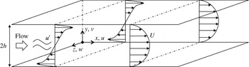
A schematic of the channel-flow configuration is shown in figure 1. The bulk velocity,
 $U_{b}$
, and the channel half-height,
 $h$
, are selected as the reference scales. This yields the definition of the bulk Reynolds number,
 $Re=hU_{b}/\unicode[STIX]{x1D708}$
, where
 $\unicode[STIX]{x1D708}$
is the fluid total kinematic viscosity. In addition, the ratio of the polymer relaxation time
 $\unicode[STIX]{x1D706}$
to the flow time scale
 $h/U_{b}$
defines the Weissenberg number,
 $Wi=\unicode[STIX]{x1D706}U_{b}/h$
. The flow is assumed to be periodic in the streamwise
 $(x)$
and spanwise
 $(z)$
directions, and bounded by no-slip walls in the wall-normal coordinate at
 $y=0$
and
 $y=2$
.
Schematic of flow configuration.

2.1 Governing equations
In order to model the influence of polymer additives, the incompressible Navier–Stokes equations are supplemented by an additional force term,
 $$\begin{eqnarray}\displaystyle & \displaystyle \frac{\unicode[STIX]{x2202}u_{i}}{\unicode[STIX]{x2202}x_{i}}=0, & \displaystyle\end{eqnarray}$$
 $$\begin{eqnarray}\displaystyle & \displaystyle \frac{\unicode[STIX]{x2202}u_{i}}{\unicode[STIX]{x2202}t}+u_{j}\frac{\unicode[STIX]{x2202}u_{i}}{\unicode[STIX]{x2202}x_{j}}=-\frac{\unicode[STIX]{x2202}p}{\unicode[STIX]{x2202}x_{i}}+\frac{\unicode[STIX]{x1D6FD}}{Re}\frac{\unicode[STIX]{x2202}^{2}u_{i}}{{\unicode[STIX]{x2202}x_{j}}^{2}}+\underbrace{\frac{1-\unicode[STIX]{x1D6FD}}{Re}\frac{\unicode[STIX]{x2202}\unicode[STIX]{x1D749}_{ij}}{\unicode[STIX]{x2202}x_{j}}}_{f_{i}}. & \displaystyle\end{eqnarray}$$
In the above equations,
 $\unicode[STIX]{x1D6FD}$
is the ratio of the solvent to the zero shear total viscosity,
 $\unicode[STIX]{x1D6FD}\equiv \unicode[STIX]{x1D707}_{s}/\unicode[STIX]{x1D707}_{0}=\unicode[STIX]{x1D707}_{s}/(\unicode[STIX]{x1D707}_{s}+\unicode[STIX]{x1D707}_{p})$
, where
 $\unicode[STIX]{x1D707}_{s}$
and
 $\unicode[STIX]{x1D707}_{p}$
are the individual contributions to the total viscosity by the Newtonian solvent and the polymer, respectively. The viscosity ratio can also be interpreted as the polymer concentration in the solution. In the current study,
 $\unicode[STIX]{x1D6FD}$
is assumed constant in time and homogeneous in space. In addition to the polymeric effect on viscosity, the polymer force is included in the momentum equation as the divergence of a polymer stress,
 $f_{i}=\unicode[STIX]{x2202}\unicode[STIX]{x1D749}_{ij}/\unicode[STIX]{x2202}x_{j}$
.
The viscoelastic stress is related to the polymer conformation tensor via the FENE-P closure,
 $$\begin{eqnarray}\displaystyle \left.\begin{array}{@{}c@{}}\displaystyle \unicode[STIX]{x1D749}_{ij}=\frac{1}{Wi}\left(\frac{\unicode[STIX]{x1D624}_{ij}}{\unicode[STIX]{x1D713}}-\frac{\unicode[STIX]{x1D6FF}_{ij}}{a}\right),\\ \displaystyle \unicode[STIX]{x1D713}=1-\frac{\unicode[STIX]{x1D624}_{kk}}{L_{max}^{2}},\\ \displaystyle a=1-\frac{3}{L_{max}^{2}},\end{array}\right\} & & \displaystyle\end{eqnarray}$$
where
 $L_{max}$
is the maximum extensibility of the polymer. The conformation tensor
 $\unicode[STIX]{x1D624}_{ij}$
describes the ensemble-averaged deformation of the polymer molecules
 $\langle \boldsymbol{q}_{i}\boldsymbol{q}_{j}\rangle$
, where
 $\boldsymbol{q}_{i}$
is the end-to-end vector of individual chains. The evolution equation for the conformation tensor features the upper convective derivative of
 $\unicode[STIX]{x1D624}_{ij}$
, which accounts for transport and deformation, and stress relaxation,
 $$\begin{eqnarray}\frac{\unicode[STIX]{x2202}\unicode[STIX]{x1D624}_{ij}}{\unicode[STIX]{x2202}t}+u_{k}\frac{\unicode[STIX]{x2202}\unicode[STIX]{x1D624}_{ij}}{\unicode[STIX]{x2202}x_{k}}=\unicode[STIX]{x1D624}_{kj}\frac{\unicode[STIX]{x2202}u_{i}}{\unicode[STIX]{x2202}x_{k}}+\unicode[STIX]{x1D624}_{ik}\frac{\unicode[STIX]{x2202}u_{j}}{\unicode[STIX]{x2202}x_{k}}-\unicode[STIX]{x1D749}_{ij}.\end{eqnarray}$$
Flow variables can be decomposed into their mean value and a perturbation,
 $\unicode[STIX]{x1D703}=\overline{\unicode[STIX]{x1D703}}+\unicode[STIX]{x1D703}^{\prime }$
where overline denotes averaging in the homogeneous streamwise and spanwise directions only. As a result,
 $\overline{\unicode[STIX]{x1D703}}$
is generally time dependent. In the limit of small-amplitude linear perturbations, the decomposition is expressed as
 $\unicode[STIX]{x1D703}=\unicode[STIX]{x1D6E9}+\unicode[STIX]{x1D703}^{\prime }$
, where uppercase denotes the base state which is unchanging in time.
2.2 Numerical method
The Navier–Stokes equations (2.2) are discretized using a control volume formulation (Rosenfeld, Kwak & Vinokur Reference Rosenfeld, Kwak and Vinokur1991), and are advanced using a fractional step algorithm. The temporal discretization of the advection term uses an explicit Adams–Bashforth scheme, while the diffusion and polymer stress terms are treated implicitly using Crank–Nicolson. An intermediate velocity is first evaluated using an estimate of the pressure from the previous time step, and is subsequently projected onto a solenoidal field using the pressure correction. The elliptic equation governing the pressure correction is solved using Fourier transform in the spanwise and streamwise directions, and a tridiagonal inversion in the wall-normal coordinate.
The numerical solution of the conformation tensor equation (2.4) is similar to previous studies (Min et al. Reference Min, Yoo, Choi and Joseph2003; Dubief et al. Reference Dubief, Terrapon, White, Shaqfeh, Moin and Lele2005; Kim et al. Reference Kim, Li, Sureshkumar, Balachandar and Adrian2007). Time integration is performed using a low-storage third-order accurate Runge–Kutta method. Within each Runge–Kutta substep, the advection terms are treated using Adams–Bashforth and both the polymer stretch and relaxation are discretized using Crank–Nicolson.
The hyperbolic nature of the evolution equation of the conformation tensor can give rise to numerical instability (Chilcott & Rallison Reference Chilcott and Rallison1988), particularly at high Weissenberg number. Various methods have been proposed in order to address this issue and to ensure that the conformation tensor remains positive definite. One approach uses slope limiting schemes to discretize the advection term (Vaithianathan & Collins Reference Vaithianathan and Collins2003; Vaithianathan et al.
Reference Vaithianathan, Robert, Brasseur and Collins2006); another adopts a log-conformation representation (Fattal & Kupferman Reference Fattal and Kupferman2005). In the present study, the advection term in (2.4) is discretized using a third-order accurate weighted essentially non-oscillating (WENO) scheme (Shu Reference Shu2009). Following the procedure by Min, Yoo & Choi (Reference Min, Yoo and Choi2001) a local artificial diffusion (LAD) term,
 $\tilde{\unicode[STIX]{x1D705}}\unicode[STIX]{x0394}x_{i}^{2}(\unicode[STIX]{x2202}^{2}\unicode[STIX]{x1D624}_{lm}/\unicode[STIX]{x2202}x_{i}^{2})$
, is introduced on the right-hand side of (2.4) where
 $\unicode[STIX]{x0394}x_{i}$
is the grid spacing in the
 $i$
-direction and
 $\unicode[STIX]{x1D705}\equiv \tilde{\unicode[STIX]{x1D705}}\unicode[STIX]{x0394}x_{i}^{2}$
is the diffusivity. This term selectively acts at grid points where the polymer conformation is no longer positive definite, and hence its effect is minimized (Min et al.
Reference Min, Yoo, Choi and Joseph2003; Dubief et al.
Reference Dubief, White, Terrapon, Shaqfeh, Moin and Lele2004). Use of LAD was favourably contrasted to global diffusion by Li, Sureshkumar & Khomami (Reference Li, Sureshkumar and Khomami2006), and was adopted successfully in simulations of polymeric turbulent flows (e.g. Min et al.
Reference Min, Yoo, Choi and Joseph2003; Dubief et al.
Reference Dubief, White, Terrapon, Shaqfeh, Moin and Lele2004; Dimitropoulos et al.
Reference Dimitropoulos, Dubief, Shaqfeh, Moin and Lele2005), so long as the local effective Schmidt number,
 $Sc\equiv \unicode[STIX]{x1D708}/\unicode[STIX]{x1D705}$
, is larger than unity. This condition is satisfied in all the present simulations.
Two classes of simulations were performed: the first examines the linear growth and nonlinear saturation of two-dimensional Tollmien–Schlichting waves, and the second evaluates their secondary instability and full nonlinear breakdown to turbulence. The LAD term was not active in any of the former simulations. It was only activated in simulations of three-dimensional breakdown, in the very late stages when turbulent spots are formed, and affected less than 6 % of grid points at the highest elasticity and lower percentages for the smaller
 $Wi$
. In the final fully turbulent states, less than 2 % of grid points were affected. These levels are well within the guidelines by Dubief et al. (Reference Dubief, Terrapon, White, Shaqfeh, Moin and Lele2005) who simulated fully turbulent viscoelastic flows at similar Reynolds and Weissenberg numbers, and lower than in previous direct numerical simulations (DNS) of bypass transition (Agarwal et al.
Reference Agarwal, Brandt and Zaki2014).
The computational domains and grid parameters for the two classes of simulations are provided in table 1. In both bases, the grid spacing is uniform in the streamwise and spanwise directions. In the wall-normal direction, a uniform grid was used in the primary simulations and a hyperbolic tangent function was adopted for grid stretching in the transitional simulations. The grid spacings in viscous units are normalized by the friction velocity during the fully turbulent state of a reference Newtonian simulation.
Parameters of the computational domain. Grid resolution is normalized by the Newtonian viscous length scale,
 $\unicode[STIX]{x1D708}/u_{\unicode[STIX]{x1D70F}}$
where
 $u_{\unicode[STIX]{x1D70F}}$
is frictional velocity and
 $\unicode[STIX]{x1D708}$
is kinematic viscosity.

2.3 Initial condition: base flow and Tollmien–Schlichting wave
The initial flow field is a superposition of a laminar base state and an infinitesimal Tollmien–Schlichting perturbation. The former is the viscoelastic Poiseuille flow solution for a FENE-P fluid (see e.g. Cruz, Pinho & Oliveira Reference Cruz, Pinho and Oliveira2005), which is summarized here for completeness.
The base flow profile is given by,
 $$\begin{eqnarray}\displaystyle U(y) & = & \displaystyle \frac{Re}{2\unicode[STIX]{x1D6FD}}\frac{\text{d}P}{\text{d}x}(y^{2}-2y)-\frac{1-\unicode[STIX]{x1D6FD}}{\unicode[STIX]{x1D6FD}}\frac{3}{8J_{0}} [F^{+}(y)G^{-}(y)+F^{-}(y)G^{+}(y)\nonumber\\ \displaystyle & & \displaystyle -\,F^{+}(0)G^{-}(0)-F^{-}(0)G^{+}(0)],\end{eqnarray}$$
 $$\begin{eqnarray}\displaystyle & \displaystyle F^{\pm }(y)=\left(J_{0}(y-1)\pm \sqrt{J_{0}^{2}(y-1)^{2}+K_{0}^{3}}\right)^{1/3}, & \displaystyle\end{eqnarray}$$
 $$\begin{eqnarray}\displaystyle & \displaystyle G^{\pm }(y)=3J_{0}(y-1)\pm \sqrt{J_{0}^{2}(y-1)^{2}+K_{0}^{3}}, & \displaystyle\end{eqnarray}$$
 $$\begin{eqnarray}\displaystyle & \displaystyle J_{0}=\frac{Re}{4\unicode[STIX]{x1D6FD}}\left(\frac{L_{max}}{a\,Wi}\right)^{2}\frac{\text{d}P}{\text{d}x}, & \displaystyle\end{eqnarray}$$
 $$\begin{eqnarray}\displaystyle & \displaystyle K_{0}=\frac{1}{6\unicode[STIX]{x1D6FD}}\left(\frac{L_{max}}{a\,Wi}\right)^{2}. & \displaystyle\end{eqnarray}$$
All components of polymeric stress tensor associated with this parallel base state vanish except
 $\unicode[STIX]{x1D61B}_{xx}$
and
 $\unicode[STIX]{x1D61B}_{xy}$
,
 $$\begin{eqnarray}\unicode[STIX]{x1D61B}_{yy}=\unicode[STIX]{x1D61B}_{zz}=\unicode[STIX]{x1D61B}_{yz}=\unicode[STIX]{x1D61B}_{xz}=0,\end{eqnarray}$$
The shear component of the stress is a solution to the cubic equation,
 $$\begin{eqnarray}T_{xy}^{3}+3K_{0}\unicode[STIX]{x1D61B}_{xy}-2J_{0}(y-1)=0.\end{eqnarray}$$
Finally, the normal stress is computed from the relation,
 $$\begin{eqnarray}\unicode[STIX]{x1D61B}_{xx}=2\,a\,Wi\,T_{xy}^{2},\end{eqnarray}$$
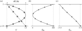
and the conformation tensor is evaluated using (2.3). The base state velocity profiles for Newtonian and non-Newtonian flows are plotted in figure 2, as well as the trace and shear component of the conformation tensor of the latter configuration.
Wall-normal profiles of the base state. (a) Mean velocity,
 $U$
, and its gradient,
 $\text{d}U/\text{d}y$
; (b) trace of the conformation tensor,
 $\unicode[STIX]{x1D60A}_{kk}$
; (c) shear component of the conformation tensor,
 $\unicode[STIX]{x1D60A}_{xy}$
. —○— Newtonian flow; —▵— viscoelastic flow at
 $Re=4667$
,
 $Wi=6.67$
,
 $L_{max}=100$
and
 $\unicode[STIX]{x1D6FD}=0.9$
.

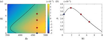
Stability diagram for viscoelastic FENE-P channel flow at
 $\unicode[STIX]{x1D6FD}=0.9$
and
 $L_{max}=100$
. (a) Contours of the maximum, two-dimensional temporal growth rate,
 $\unicode[STIX]{x1D70E}_{i}$
, as a function of
 $Re$
and
 $Wi$
at
 $k_{x}=k_{x,max}$
; (b)
 $\unicode[STIX]{x1D70E}_{i}$
versus
 $Wi$
at
 $Re=4667$
with (— ⋅ —)
 $k_{x}=k_{x,max}$
and (——)
 $k_{x}=1.0$
. Filled circles identify the
 $(Re,Wi)$
pairs for the present simulations.

The initial disturbance is a two-dimensional Tollmien–Schlichting wave, which is an eigenmode of the linear stability equations. The eigenvalue problem and its solution procedure are described in appendix A. For every pair of Reynolds and Weissenberg numbers of interest, the eigenvalue problem was solved over a range of streamwise wavenumbers,
 $k_{x}$
. The two-dimensional mode with the largest temporal growth rate,
 $\unicode[STIX]{x1D70E}_{i}$
, was recorded and the results are plotted in figure 3(a) for elastic parameters
 $\unicode[STIX]{x1D6FD}=0.9$
and
 $L_{max}=100$
. Consistent with previous studies, elasticity has a non-monotonic effect on flow stability (Larson Reference Larson1992; Sadanandan & Sureshkumar Reference Sadanandan and Sureshkumar2002; Zhang et al.
Reference Zhang, Lashgari, Zaki and Brandt2013). The neutral curve is marked by the dark line in the figure. To its left, the flow is asymptotically stable to small-amplitude disturbances and is otherwise unstable.
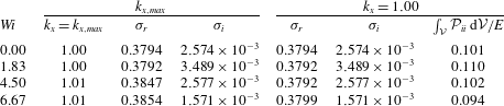
The Reynolds–Weissenberg number pairs of interest are marked on the figure and are also listed in table 2. They are
 $Re=4667$
and
 $Wi=\{0,1.83,4.50,6.67\}$
. The streamwise wavenumber that exhibits maximum amplification,
 $k_{x,max}$
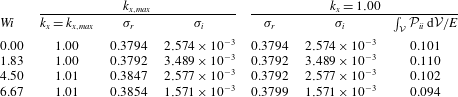
, for each of these conditions is also listed in the table. Since it is inappreciably changed by elasticity, we elected to simulate
 $k_{x}=1.00$
, which unifies the streamwise domain size in all simulations. A comparison of the growth rates associated with
 $k_{x,max}$
and
 $k_{x}=1.00$
is provided in figure 3(b) and table 2.
The effect of elasticity on transition will be through modification of the growth rate of the primary TS wave, and also by altering its secondary instability. Separating these two effects is not straightforward, and motivates the present choice of parameters. The Newtonian condition is in the supercritical regime, and is considered a reference case. The viscoelastic simulations correspond to three unstable growth rates of the primary TS wave: the peak value at the Reynolds number of interest; an equal growth rate to the Newtonian condition; and a lower growth rate than Newtonian. The choice of the second case is aimed to highlight the influence of elasticity on the secondary instability.
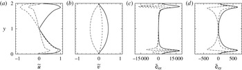
Wall-normal profile of the Tollmien–Schlichting wave at
 $Re=4667$
,
 $Wi=6.67$
,
 $\unicode[STIX]{x1D6FD}=0.9$
,
 $L_{max}=100$
. (a) Streamwise and (b) wall-normal velocity; (c) streamwise and (d) shear components of the conformation tensor. (– – –) Real, (— ⋅ —) imaginary and (——) absolute values are plotted.

Comparison of the maximum temporal eigenvalue,
 $\unicode[STIX]{x1D70E}=\unicode[STIX]{x1D70E}_{r}+\text{i}\unicode[STIX]{x1D70E}_{i}$
, at
 $k_{x}=k_{x,max}$
and
 $k_{x}=1.0$
, for the
 $(Re,Wi)$
pairs of the present simulations.
 $Re=4667$
,
 $\unicode[STIX]{x1D6FD}=0.9$
,
 $L_{max}=100$
.
For each mode of interest, the linear stability analysis provides the velocity profile
 $\tilde{u} _{i}(y)$
, conformation tensor profile
 $\tilde{\unicode[STIX]{x1D624}}_{ij}(y)$
, and complex eigenfrequency
 $\unicode[STIX]{x1D70E}=\unicode[STIX]{x1D70E}_{r}+\text{i}\unicode[STIX]{x1D70E}_{i}$
. The mode shape of the two-dimensional Tollmien–Schlichting wave at
 $Wi=6.67$
is shown in figure 4. The initial condition for the DNS is then constructed from a superposition of the base state and the linear instability mode,
 $$\begin{eqnarray}\displaystyle & \displaystyle u_{i}=U_{i}+u_{i}^{\prime }=U_{i}+\unicode[STIX]{x1D716}\text{Re}\{\tilde{u} _{i}\text{e}^{\unicode[STIX]{x1D70E}_{i}t}\text{e}^{\text{i}(k_{x}x-\unicode[STIX]{x1D70E}_{r}t)}\}, & \displaystyle\end{eqnarray}$$
 $$\begin{eqnarray}\displaystyle & \displaystyle \unicode[STIX]{x1D624}_{ij}=\unicode[STIX]{x1D60A}_{ij}+\unicode[STIX]{x1D624}_{ij}^{\prime }=\unicode[STIX]{x1D60A}_{ij}+\unicode[STIX]{x1D716}\text{Re}\{\tilde{\unicode[STIX]{x1D624}}_{ij}\text{e}^{\unicode[STIX]{x1D70E}_{i}t}\text{e}^{\text{i}(k_{x}x-\unicode[STIX]{x1D70E}_{r}t)}\}, & \displaystyle\end{eqnarray}$$
where
 $\unicode[STIX]{x1D716}$
is the initial disturbance amplitude and
 $t$
is zero at the initial time.
3 Results
In analogy to previous Newtonian studies, we will examine the linear growth of the primary TS wave followed by its nonlinear saturation. These computations will provide the foundation for selecting an appropriate initial condition for the subsequent simulations of secondary instability and breakdown to a fully turbulent state.
3.1 Linear growth and nonlinear energy saturation
The first set of direct numerical simulations start from the laminar base flow profile and a small-amplitude TS wave. In order to ensure that the initial stage is within the linear regime, both the velocity and conformation tensor of the perturbation must be small relative to the mean-flow values. The initial amplitude of TS wave was set to
 $\unicode[STIX]{x1D716}=0.01\,\%$
relative to the bulk velocity, which guarantees the presence of an initial linear regime during the evolution of the disturbance. The ability to reproduce the linear growth rate of a small-amplitude TS wave using a numerical solution of the full Navier–Stokes equations serves as a validation of our numerical method. In addition, it guarantees that a nonlinear state, once reached, is also a solution of the governing equations and an appropriate starting point for the subsequent transition computations.
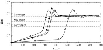
The perturbation energy density was evaluated from each of the four simulations,
 $$\begin{eqnarray}E(t)=\frac{1}{L_{x}\,L_{y}\,L_{z}}\int _{0}^{L_{z}}\int _{0}^{L_{y}}\int _{0}^{L_{x}}\frac{1}{2}({u^{\prime }}^{2}+{v^{\prime }}^{2}+{w^{\prime }}^{2})\,\text{d}x\,\text{d}y\,\text{d}z.\end{eqnarray}$$
Note that the perturbation field is initially monochromatic in
 $k_{x}$
, and has a discrete spectrum in the nonlinear regime due to the generation of higher harmonics. As such, the perturbation field was obtained by subtracting the streamwise–spanwise average from the total signal. Figure 5 shows the evolution of
 $E(t)$
from the initial time and through
 $t=4650$
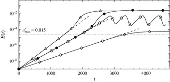
convective time units. The initial linear amplification of
 $\log (E)$
corresponds to the exponential amplification of the TS wave in all four simulations. The slopes of the curves from DNS match the predictions of linear stability theory, which are marked in the figure by dashed lines with slopes equal to
 $2\unicode[STIX]{x1D70E}_{i}$
(values of
 $\unicode[STIX]{x1D70E}_{i}$
are listed in table 2).
Evolution of the perturbation energy at
 $Re=4667$
,
 $\unicode[STIX]{x1D6FD}=0.9$
and
 $L_{max}=100$
. (—●—) Newtonian; (—▵—)
 $Wi=1.83$
; (—○—)
 $Wi=4.50$
; (—♢—)
 $Wi=6.67$
. Dashed lines mark the prediction from linear stability theory.

Zhang et al. (Reference Zhang, Lashgari, Zaki and Brandt2013) examined the change in the growth rate of the primary TS wave by evaluating the various terms in the perturbation energy budget, and a similar analysis can also be instructive in the nonlinear regime. The evolution equation for Reynolds stress is,
 $$\begin{eqnarray}\displaystyle \frac{\unicode[STIX]{x2202}\overline{u_{i}^{\prime }u_{j}^{\prime }}}{\unicode[STIX]{x2202}t} & = & \displaystyle \underbrace{-\overline{u}_{k}\frac{\unicode[STIX]{x2202}\overline{u_{i}^{\prime }u_{j}^{\prime }}}{\unicode[STIX]{x2202}x_{k}}}_{2{\mathcal{A}}_{ij}}\underbrace{-\left(\overline{u_{j}^{\prime }u_{k}^{\prime }}\frac{\unicode[STIX]{x2202}\overline{u}_{i}}{\unicode[STIX]{x2202}x_{k}}+\overline{u_{i}^{\prime }u_{k}^{\prime }}\frac{\unicode[STIX]{x2202}\overline{u}_{j}}{\unicode[STIX]{x2202}x_{k}}\right)}_{2{\mathcal{P}}_{ij}}\nonumber\\ \displaystyle & & \displaystyle \underbrace{-\,\frac{\unicode[STIX]{x2202}\overline{u_{i}^{\prime }u_{j}^{\prime }u_{k}^{\prime }}}{\unicode[STIX]{x2202}x_{k}}}_{2{\mathcal{Q}}_{ij}}\underbrace{-\left(\overline{u_{j}^{\prime }\frac{\unicode[STIX]{x2202}p^{\prime }}{\unicode[STIX]{x2202}x_{i}}}+\overline{u_{i}^{\prime }\frac{\unicode[STIX]{x2202}p^{\prime }}{\unicode[STIX]{x2202}x_{j}}}\right)}_{2\unicode[STIX]{x1D719}_{ij}}+\underbrace{\frac{\unicode[STIX]{x1D6FD}}{Re}\frac{\unicode[STIX]{x2202}^{2}\overline{u_{i}^{\prime }u_{j}^{\prime }}}{\unicode[STIX]{x2202}x_{k}^{2}}}_{2{\mathcal{D}}_{ij}}\nonumber\\ \displaystyle & & \displaystyle \underbrace{-\,2\frac{\unicode[STIX]{x1D6FD}}{Re}\overline{\frac{\unicode[STIX]{x2202}u_{j}^{\prime }}{x_{k}}\frac{\unicode[STIX]{x2202}u_{i}^{\prime }}{x_{k}}}}_{2\unicode[STIX]{x1D716}_{ij}}+\underbrace{\frac{1-\unicode[STIX]{x1D6FD}}{Re}\left(\overline{u_{j}^{\prime }\frac{\unicode[STIX]{x2202}\unicode[STIX]{x1D749}_{ik}^{\prime }}{\unicode[STIX]{x2202}x_{k}}}+\overline{u_{i}^{\prime }\frac{\unicode[STIX]{x2202}\unicode[STIX]{x1D749}_{jk}^{\prime }}{\unicode[STIX]{x2202}x_{k}}}\right)}_{2{\mathcal{W}}_{ij}}.\end{eqnarray}$$
The term
 ${\mathcal{A}}_{ij}$
is mean advection,
 ${\mathcal{P}}_{ij}$
is production,
 ${\mathcal{Q}}_{ij}$
is energy transport by fluctuations,
 $\unicode[STIX]{x1D719}_{ij}$
is pressure redistribution,
 ${\mathcal{D}}_{ij}$
is viscous diffusion,
 $\unicode[STIX]{x1D716}_{ij}$
is dissipation and
 ${\mathcal{W}}_{ij}$
is polymer work. The energy equation is obtained from (3.2) by setting
 $i=j$
,
 $$\begin{eqnarray}\displaystyle \frac{\unicode[STIX]{x2202}k}{\unicode[STIX]{x2202}t}\equiv \frac{\unicode[STIX]{x2202}\frac{1}{2}\overline{u_{i}^{\prime }u_{i}^{\prime }}}{\unicode[STIX]{x2202}t}=({\mathcal{A}}_{ii}+{\mathcal{Q}}_{ii}+\unicode[STIX]{x1D719}_{ii}+{\mathcal{P}}_{ii}+{\mathcal{D}}_{ii}+\unicode[STIX]{x1D716}_{ii}+{\mathcal{W}}_{ii}). & & \displaystyle\end{eqnarray}$$
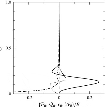
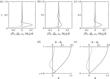
The dominant terms in (3.3) were evaluated at
 $t=1000$
, which is well within the linear regime according to figure 5. Their wall-normal profiles are plotted in figure 6 normalized by the total perturbation energy, for the case with
 $Wi=6.67$
as means of example. The production term is the largest contributor to the energy budget. Its peak is reached at
 $y/h=0.13$
, which is the height of the critical layer, or the location where the base flow speed is equal to the phase speed of the TS wave,
 $\overline{u}(y/h=0.13)=\unicode[STIX]{x1D70E}_{r}/k_{x}$
. As discussed by Zhang et al. (Reference Zhang, Lashgari, Zaki and Brandt2013), the change in the growth rate of the TS wave tracks the change in this peak production term.
Dominant terms in the perturbation kinetic energy budget (3.3) for
 $Wi=6.67$
at
 $t=1000$
, which is within the linear regime. (——)
 ${\mathcal{P}}_{ii}/E$
; (– – –)
 ${\mathcal{Q}}_{ii}/E$
; (— ⋅ —)
 $\unicode[STIX]{x1D716}_{ii}/E$
; (
 $\cdots \cdots$
)
 ${\mathcal{W}}_{ii}/E$
.

The integral of the production term at
 $t=1000$
is reported in table 2 normalized by the total perturbation energy. This quantity increases from the Newtonian to the first viscoelastic case,
 $Wi=1.83$
, which has the highest TS growth rate. Increasing the Weissenberg number further reduces
 $\unicode[STIX]{x1D70E}_{i}$
, and the integrated production also reduces. Note that when the TS growth rates of the Newtonian and viscoelastic flows are equal (
 $Wi=0.00$
and
 $4.50$
), the integrated productions are closest. These trends are therefore in agreement with the results by Zhang et al. (Reference Zhang, Lashgari, Zaki and Brandt2013).
The deviation of the energy curve in figure 5 from the initial linear slope signals the onset of nonlinear effects. In this regime, the perturbation velocities or conformation have reached an appreciable amplitude and, as a result, can generate higher harmonics and distort the base state. The base flow distortion, in turn, alters the growth rate of the TS wave. A saturation of the energy curve in figure 5 signals a balance between the rate at which perturbations extract energy from the distorted base flow and the rate at which they dissipate energy due to viscosity. This argument is based on the Newtonian energy equation which is supplemented by a polymer work term in the polymeric case which can lead to richer behaviour. Indeed only three of the four flow conditions show energy saturation,
 $Wi=\{0.00,1.83,6.67\}$
, while the viscoelastic simulation at
 $Wi=4.50$
reaches a periodic state with cycles of energy amplification and decay.
The energy of the saturated state and, as a result, the amplitude of the velocity perturbation in this regime depend on the Weissenberg number. Of the four conditions, the highest Weissenberg number simulation saturates at the lowest perturbation energy,
 $E=5.59\times 10^{-5}$
. The corresponding maximum amplitudes of the perturbation velocities are
 $u_{max}^{\prime }=1.6\,\%$
and
 $v_{max}^{\prime }=0.7\,\%$
. These peak values should be contrasted to the work by Sandham & Kleiser (Reference Sandham and Kleiser1992) who simulated K-type transition in channel flow starting from a TS wave with amplitude equal to 4.5 % of the bulk velocity. A similar initial condition to Sandham & Kleiser (Reference Sandham and Kleiser1992) is therefore not feasible in the present study, since a primary TS wave with such high peak amplitude is not realizable at the highest elasticity.
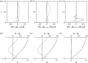
Terms in the perturbation kinetic energy budget and mean-velocity profiles in the nonlinear saturated states. (a,d) Newtonian flow at
 $t=4000$
; (b,e)
 $Wi=1.83$
at
 $t=2980$
; (c,f)
 $Wi=6.67$
at
 $t=4500$
. (a–c) Line types retain the same meaning as in figure 6. (——)
 ${\mathcal{P}}_{ii}/E$
; (– – –)
 ${\mathcal{Q}}_{ii}/E$
; (— ⋅ —)
 $\unicode[STIX]{x1D716}_{ii}/E$
; (
 $\cdots \cdots$
)
 ${\mathcal{W}}_{ii}/E$
. Panels (d–f) show (——) the velocity profile
 $U$
and (— ⋅ —) its distortion from the laminar solution,
 $\overline{u}-\overline{u}_{L}$
.

Terms in the kinetic energy budget were evaluated at the saturated state and are reported in figure 7 which contrasts the Newtonian with the low- and high-
 $Wi$
flows. In the Newtonian and weak elastic case (
 $Wi=1.83$
), the energy transport by the perturbation field becomes significant across the channel, surpassing the production term which is no longer concentrated in the near-wall region. The respective saturated states from these two simulations are qualitatively similar because the relaxation time at
 $Wi=1.83$
is short relative to the time scale of the TS wave, and elastic effects on the saturated states are inappreciable. In contrast, the terms in the kinetic energy budget of the highest
 $Wi$
condition are more akin to the profiles from linear theory, despite the fact that the energy evolution in figure 5 deviates from linear theory. The wall-normal profile of the mean velocity,
 $\overline{u}$
, is also plotted in figure 7 along with the distortion relative to the reference laminar base state,
 $\overline{u}_{L}=U(y)$
. In the Newtonian and low
 $Wi$
cases, the mean-flow distortion is appreciable and switches sign twice, near
 $y=0.2$
and
 $y=0.6$
. In contrast, the mean-flow distortion is very weak for the highest
 $Wi$
condition.
One curious observation in figure 5 is the oscillation of the energy curve when
 $Wi=4.50$
. Terms in the energy budget and the mean velocity profiles in the linear stage and at the peak and trough of the oscillation are compared in figure 8. At the energy peak, the profiles resemble those extracted from the saturated state in the Newtonian and low-
 $Wi$
cases (figure 7
a,b). However, the production term is more pronounced near the wall, and the magnitude of the nonlinear transport term is relatively weaker. The associated mean-flow distortion is also small compared to the Newtonian and lower
 $Wi$
cases. This state is not maintained, but rather gives way to a decay in the kinetic energy and a rapid shift in the budget profiles towards a new configuration that is more akin to the linear stage. For example, the negative polymer work term re-emerges in the near-wall region where the mean-flow distortion vanishes. In addition, the maximum production term increases relative to the remaining terms in the budget and will drive energy amplification at the onset of the subsequent cycle.
That the flow does not reach a constant energy state highlights the rich dynamics that ensues when elasticity is present. As the TS wave amplifies, the mean flow is distorted and, as a result, production, dissipation and polymer work are all modified. At low and high elasticity, similar to the Newtonian case, an equilibrium is reached while at the intermediate
 $Wi$
such equilibrium is not possible and the flow continues in cycles of amplification of decay.
Terms in the perturbation kinetic energy budget and mean-velocity profiles for
 $Wi=4.50$
during the periodic nonlinear state. (a) Results from the linear regime are provided for comparison. The results from the nonlinear state are shown at the local (b,d) peaks and (c,e) troughs. (a–c) Line types retain the same meaning. (——)
 ${\mathcal{P}}_{ii}/E$
; (– – –)
 ${\mathcal{Q}}_{ii}/E$
; (— ⋅ —)
 $\unicode[STIX]{x1D716}_{ii}/E$
; (
 $\cdots \cdots$
)
 ${\mathcal{W}}_{ii}/E$
. Panels (d,e) show (——) the velocity profile
 $U$
and (— ⋅ —) its distortion from the laminar solution,
 $\overline{u}-\overline{u}_{L}$
.

The nonlinear state described above remains two-dimensional and does not break down to turbulence, even though the computational domain is three-dimensional. These simulations are important for two reasons: first, they highlight the propensity of polymers to suppress the disturbance energy in nonlinear regime, which is instrumental to understanding the later stages of transition. Second, these simulations provide an accurate initial base state to which a small-amplitude three-dimensional perturbation can be added in order to study the onset of secondary instability and breakdown to turbulence.
3.2 Secondary instabilities
The simulations of the secondary instability start from the flow fields reported in § 3.1. The flow velocities, pressure and conformation tensor are extracted at
 $t=t^{\ast }$
which is defined as the time where
 $E(t^{\ast })=2.25\times 10^{-5}$
. In all simulations, this state precedes the onset of any appreciable deviation from the linear energy curve, or any pronounced nonlinear effects. In the Newtonian case, this energy level corresponds to
 $u_{max}^{\prime }=0.015U_{b}$
, or
 $u_{max}^{\prime }=0.01U_{c}$
where
 $U_{c}$
is the centreline velocity. The fields are supplemented with a zero-mean uncorrelated velocity perturbation with magnitude less than
 $0.001U_{c}$
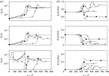
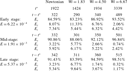
. The evolution of the total perturbation energy is shown in figure 9, and is separated into the contributions of the three components of the velocity vector in figure 10. On figure 9, three energy levels are marked and identified as early, mid- and late stages of transition. The energy level and time associated with each of these stages are detailed in table 3, and will serve as landmarks for the discussion.
The initial evolution of the total energy in figure 9 preserves the linear growth of the primary TS wave due to the choice of
 $t^{\ast }$
and despite the addition of white noise. The same region in figure 10(a) confirms that both the streamwise and wall-normal velocities are amplifying according to linear theory, while the small-amplitude initial white noise that was introduced in the spanwise component simply decays (see inset). After some time, the energy amplification rate in figure 9 increases appreciably, which marks the onset of secondary instability. It is important to note that, while the kinetic energy is lowest for
 $Wi=6.67$
when secondary instability sets in, the perturbation to the conformation tensor is largest for this case.
The increase in the slope of
 $E(t)$
at the point of secondary instability resembles the behaviour at the start of nonlinear saturation (§ 3.1), but there the flow remained two-dimensional. Here, on the other hand, three-dimensionality has set in and
 $E_{z}$
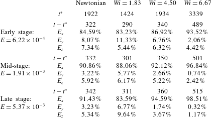
also amplifies as shown in figure 10(a). A helpful way to highlight the change from a two- to three-dimensional perturbation field is to plot the fraction of the total energy due to each velocity component (figure 10
b). In the linear regime, the energy distribution between the streamwise and wall-normal components is constant, as determined by linear theory, and the spanwise component is absent. Once the secondary instability starts to amplify, so does the fraction of the total perturbation energy due to the spanwise velocity. In fact, both
 $E_{x}$
and
 $E_{z}$
amplify, followed by a decay in
 $E_{y}$
, independent of the fluid elasticity. A qualitative difference between the Newtonian and viscoelastic cases is observed at long time, where
 $E_{x}$
in the Newtonian case represents a smaller fraction of the total perturbation energy in the final state. On the other hand, it is a more appreciable fraction in the viscoelastic flows, and this fraction increases with
 $Wi$
. A quantitative comparison of the changes in energy and it distribution among the three components is provided in table 3. These trends will be explained with reference to the flow structures that amplify during the transition process.
Evolution of the perturbation kinetic energy at
 $Re=4667$
,
 $\unicode[STIX]{x1D6FD}=0.9$
and
 $L_{max}=100$
after the addition of background white noise at
 $t-t^{\ast }=0$
. (—●—) Newtonian; (—▵—)
 $Wi=1.83$
; (—○—)
 $Wi=4.50$
; (—♢—)
 $Wi=6.67$
.

Evolution of the perturbation kinetic energy at
 $Re=4667$
,
 $\unicode[STIX]{x1D6FD}=0.9$
and
 $L_{max}=100$
after the addition of background white noise at
 $t-t^{\ast }=0$
. (a) Energy due to each velocity component and (b) the respective fractions of the total energy. (—●—) Newtonian; (—▵—)
 $Wi=1.83$
; (—○—)
 $Wi=4.50$
; (—♢—)
 $Wi=6.67$
.

Fraction of the total perturbation energy due to each component of the velocity vector at the early, mid- and late stages of transition.
Despite being short lived, the development of secondary instabilities has been studied in detail in Newtonian flows. It is characterized by the generation and amplification of near-wall vortical structures which are initially
 $\unicode[STIX]{x1D6EC}$
-shaped and selectively develop into hairpin vortices prior to breakdown to turbulence. In Newtonian flows, these dynamics take place near the peak of the energy evolution curve (see e.g. Sandham & Kleiser Reference Sandham and Kleiser1992; Sayadi, Hamman & Moin Reference Sayadi, Hamman and Moin2013).
Plan views and energy spectra during the early stage of transition. Left panels show contours of
 $-0.01<v^{\prime }<0.01$
at
 $y=0.12$
. Right panels show the streamwise-averaged energy spectra,
 $\overline{E_{x}}$
, as a function of the integer spanwise wavenumber,
 $n_{k_{z}}\equiv k_{z}L_{z}/2\unicode[STIX]{x03C0}$
. (a) Newtonian; (b)
 $Wi=1.83$
; (c)
 $Wi=4.50$
; (d)
 $Wi=6.67$
.

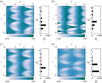
The early stage secondary instability of the TS wave is visualized in figure 11 using contours of the wall-normal velocity perturbation. The two-dimensional waves have been deformed in the span, and their shape already has the appearance of
 $\unicode[STIX]{x1D6EC}$
-shaped structures. Their arrangement demonstrates that transition in the Newtonian and viscoelastic cases is H-type, as inferred from the staggering in the spanwise direction. The streamwise subharmonic nature of the secondary instability is thus preserved independent of
 $Wi$
. The results are consistent with the literature, where H-type breakdown is commonly reported when the two-dimensional instability is moderate (Kleiser & Zang Reference Kleiser and Zang1991; White Reference White2006; Sayadi et al.
Reference Sayadi, Hamman and Moin2013), and in the present case it is approximately
 $1\,\%$
of the mean-flow speed. However elasticity alters the spanwise wavelength of the secondary instability and, as a result, of the width of the
 $\unicode[STIX]{x1D6EC}$
-structures.
Top view of
 $\unicode[STIX]{x1D6EC}$
-shaped vortices during the mid-stage of transition. The vortices are visualized using the
 $\unicode[STIX]{x1D706}_{2}$
vortex-identification criterion with thresholds
 $\unicode[STIX]{x1D706}_{2}=\{-0.1,-0.14,-0.1,-0.05\}$
. (a) Newtonian; (b)
 $Wi=1.83$
; (c)
 $Wi=4.50$
; (d)
 $Wi=6.67$
.

A typical ratio of spanwise to streamwise wavelengths is
 $\unicode[STIX]{x1D706}_{z}/\unicode[STIX]{x1D706}_{x}=0.7$
for H-type transition in Newtonian flow (see e.g. White Reference White2006, and present figure 12). In the present simulations,
 $\unicode[STIX]{x1D706}_{z}/\unicode[STIX]{x1D706}_{x}=0.66$
for the Newtonian flow. As a result three
 $\unicode[STIX]{x1D6EC}$
structures are formed across the span at every streamwise position, and the same spacing also emerges at the intermediate
 $Wi=4.50$
. When elasticity is weak (
 $Wi=1.83$
) the secondary instability is slightly narrower,
 $\unicode[STIX]{x1D706}_{z}/\unicode[STIX]{x1D706}_{x}=0.5$
; and when elasticity is high (
 $Wi=6.67$
) the instability becomes relatively wider,
 $\unicode[STIX]{x1D706}_{z}/\unicode[STIX]{x1D706}_{x}=0.8$
, with only two
 $\unicode[STIX]{x1D6EC}$
structures in the span. The size of the ensuing secondary instability can be clearly identified from the energy spectra,
 $\overline{E}_{x}(n_{k_{z}})$
, where
 $n_{k_{z}}$
is the integer spanwise wavenumber. In figure 11, the spectra were computed from the streamwise velocity perturbation and averaged in the streamwise direction. The peak energy first shifts from the integer wavenumber
 $n_{k_{z}}=3$
to a higher value (
 $n_{k_{z}}=4$
for
 $Wi=1.83$
), and then to lower wavenumbers as the
 $Wi$
is further increased. For
 $Wi=6.67$
, the peak energy is recorded at
 $n_{k_{z}}=2$
and its first harmonic due to the elongation of
 $\unicode[STIX]{x1D6EC}$
-structures in the streamwise direction.
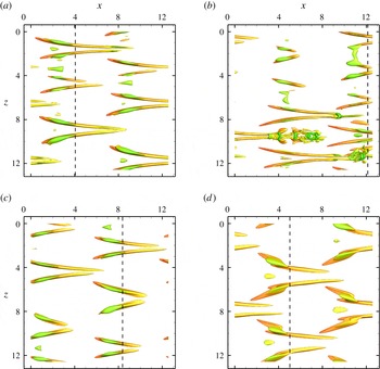
As the secondary instability intensifies,
 $\unicode[STIX]{x1D6EC}$
-shaped vortical structures start to take form during the mid-stage of transition. They are visualized in figure 12 using the
 $\unicode[STIX]{x1D706}_{2}$
vortex identification criterion. The
 $\unicode[STIX]{x1D706}_{2}$
criterion is defined as the second eigenvalue of the tensor,
 $\unicode[STIX]{x1D61A}_{ik}\unicode[STIX]{x1D61A}_{kj}+\unicode[STIX]{x1D619}_{ik}\unicode[STIX]{x1D619}_{kj}$
, where
 $\unicode[STIX]{x1D61A}_{ij}$
and
 $\unicode[STIX]{x1D619}_{ij}$
are the symmetric and antisymmetric parts of the velocity gradient tensor (Jeong & Hussain Reference Jeong and Hussain1995). Elasticity affects both the spanwise scale of the vortices and also their strength. For example, the threshold for the vortex identification criterion in figure 12 was initially increased relative to the Newtonian value when plotting the results for
 $Wi=1.83$
and subsequently reduced at higher elasticities. It is important to note that the perturbation energy level is equal among all four conditions at this stage in the transition process (
 $E=1.91\times 10^{-3}$
), although it is distributed differently among the three velocity components.
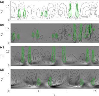
End views of the perturbation velocity field near the
 $\unicode[STIX]{x1D6EC}$
-structures during the mid-stage of transition. The streamwise locations of the planes are marked by dashed lines in figure 12. (a) Newtonian; (b)
 $Wi=1.83$
; (c)
 $Wi=4.50$
; (d)
 $Wi=6.67$
. Thick green line is a cut through the
 $\unicode[STIX]{x1D6EC}$
-structures; flood contours are
 $-0.5\leqslant u^{\prime }\leqslant 0.5$
and arrows denote the in-plane
 $(\boldsymbol{v}^{\prime },\boldsymbol{w}^{\prime })$
vectors.

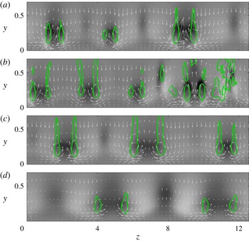
A cross-flow plane which intersects the legs of the
 $\unicode[STIX]{x1D6EC}$
-shaped structures is shown in figure 13. When the legs of the
 $\unicode[STIX]{x1D6EC}$
-structures are wider in the span, the ejection event between the long legs is less intense, as shown by the velocity vectors in the cross-flow plane. Both the
 $\boldsymbol{v}$
- and
 $\boldsymbol{w}$
-vectors are thus shortest at
 $Wi=6.67$
– a trend which is consistent with lower
 $E_{y}$
and
 $E_{z}$
in figure 10(a). The outcome is a weaker negative
 $u$
-perturbation field between the legs of the
 $\unicode[STIX]{x1D6EC}$
-structures, although
 $E_{x}$
reaches a commensurate level among all flow conditions (figure 10
a). Therefore, the positive
 $u$
-perturbation associated with sweep motion is enhanced at the highest Weissenberg number.
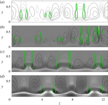
The streamwise conformation field,
 $\unicode[STIX]{x1D624}_{xx}^{\prime }$
, at the same instance as figure 13 is shown in figure 14. A pronounced sheet of positive and negative
 $\unicode[STIX]{x1D624}_{xx}^{\prime }$
is observed near the wall, and undulates in the spanwise direction. The sheet itself is due to the primary Tollmien–Schlichting wave, which is a spanwise vorticity perturbation superimposed onto the mean shear. This connection was explained by Page & Zaki (Reference Page and Zaki2015) in the more canonical setting of a spanwise Gaussian vortex in homogeneous shear. Two key effects lead to this phenomenology: (i) the action of the spanwise vorticity perturbation onto the large mean
 $\unicode[STIX]{x1D60A}_{xx}$
and (ii) the action of the mean shear on the perturbation in the polymer conformation (for details see Page & Zaki Reference Page and Zaki2015). The sheet of
 $\unicode[STIX]{x1D624}_{xx}^{\prime }$
is subsequently distorted by the secondary instability as shown in figure 14, being displaced outward with ejections and closer to the wall with sweep events.
End views of the perturbation in the conformation field,
 $\unicode[STIX]{x1D624}_{xx}^{\prime }$
near the
 $\unicode[STIX]{x1D6EC}$
-structures during the mid-stage of transition. The streamwise locations of the planes are marked by dashed lines in figure 12. (a) Newtonian; (b)
 $Wi=1.83$
; (c)
 $Wi=4.50$
; (d)
 $Wi=6.67$
. Thick green line is a cut through the
 $\unicode[STIX]{x1D6EC}$
-structures; flood contours are
 $-400\leqslant \unicode[STIX]{x1D624}_{xx}^{\prime }\leqslant 400$
and contour lines denote
 $u^{\prime }$
with spacing equal to
 $4\times 10^{-1}$
.

Since the base state and the TS wave are two-dimensional, the only contributions to
 $\unicode[STIX]{x1D624}_{xz}$
and
 $\unicode[STIX]{x1D624}_{yz}$
are due to the secondary instability. For example, figure 15 shows contours of conformation field in the cross-flow plane, and clearly captures the increase in
 $\unicode[STIX]{x1D624}_{yz}^{\prime }$
at the higher Weissenberg number. The anti-symmetry around the legs of the
 $\unicode[STIX]{x1D6EC}$
-structures is consistent with a kinematic interpretation of the sweep event: at the outer boundaries of both legs, the perturbation to the conformation is a sweep towards the wall. However, that sweep is in the negative
 $z$
-direction near the right leg and in the positive direction at the opposite side.
End views of the perturbation in the conformation field,
 $\unicode[STIX]{x1D624}_{yz}^{\prime }$
near the
 $\unicode[STIX]{x1D6EC}$
-structures during the mid-stage of transition. The streamwise locations of the planes are marked by dashed lines in figure 12. (a) Newtonian; (b)
 $Wi=1.83$
; (c)
 $Wi=4.50$
; (d)
 $Wi=6.67$
. Thick green line is a cut through the
 $\unicode[STIX]{x1D6EC}$
-structures; flood contours are
 $-100\leqslant \unicode[STIX]{x1D624}_{yz}^{\prime }\leqslant 100$
and contour lines denote
 $u^{\prime }$
with spacing equal to
 $4\times 10^{-1}$
.

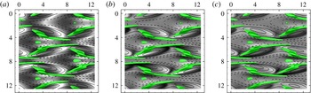
Top views of the perturbation field at
 $Wi=6.67$
are shown in figure 16. The three panels show the contours of
 $\unicode[STIX]{x1D624}_{xx}^{\prime }$
,
 $\unicode[STIX]{x1D624}_{yz}^{\prime }$
and
 $\unicode[STIX]{x1D624}_{xz}^{\prime }$
and are overlaid with the
 $\unicode[STIX]{x1D6EC}$
-structures. The first two components were discussed above, and are included in this figure for completeness. The third component,
 $\unicode[STIX]{x1D624}_{xz}^{\prime }$
, exhibits anti-symmetry relative to each leg and also across the centre of the entire
 $\unicode[STIX]{x1D6EC}$
-structure. At the outer edges, the sign of
 $\unicode[STIX]{x1D624}_{xz}^{\prime }$
mirrors the high-speed streaks which are aligned with the
 $\unicode[STIX]{x1D6EC}$
-structures towards negative-
 $z$
at right and positive-
 $z$
at left. Within the ejection zone, the sign of the conformation field is reversed because it is effected by the local streaks which are low-speed relative to the base flow.
Top views (
 $y=0.12$
) of the perturbation in the conformation field near the
 $\unicode[STIX]{x1D6EC}$
-structures during the mid-stage of transition at the highest elasticity,
 $Wi=6.67$
. Thick green line is a cut through the
 $\unicode[STIX]{x1D6EC}$
-structures, and line contours denote
 $u^{\prime }$
with spacing equal to
 $4\times 10^{-1}$
. Flood contours denote (a)
 $-400\leqslant \unicode[STIX]{x1D624}_{xx}^{\prime }\leqslant 400$
, (b)
 $-100\leqslant \unicode[STIX]{x1D624}_{yz}^{\prime }\leqslant 100$
and (c)
 $-4\leqslant \unicode[STIX]{x1D624}_{xz}^{\prime }\leqslant 4$
.

Since the
 $\unicode[STIX]{x1D6EC}$
-structures become elongated in the streamwise direction, it is important to examine the associated streamwise vorticity,
 $\unicode[STIX]{x1D714}_{x}^{\prime }$
and in the viscoelastic cases the streamwise polymer torque,
 $\unicode[STIX]{x1D712}_{x}^{\prime }$
. The term ‘polymer torque’ refers to the polymeric contribution to the vorticity evolution equation, and is derived by taking the curl of the polymer force in the momentum equation,
 $\unicode[STIX]{x1D712}_{i}^{\prime }\equiv \unicode[STIX]{x1D716}_{ijk}\,\unicode[STIX]{x2202}f_{k}^{\prime }/\unicode[STIX]{x2202}x_{j}$
where
 $f_{k}^{\prime }=\unicode[STIX]{x2202}\unicode[STIX]{x1D749}_{km}^{\prime }/\unicode[STIX]{x2202}x_{m}$
. It is directly proportional to the toque exerted on a fluid element by the polymer forces (Page & Zaki Reference Page and Zaki2015). In the streamwise direction, the evolution equation for
 $\unicode[STIX]{x1D714}_{x}^{\prime }$
is,
 $$\begin{eqnarray}\frac{\unicode[STIX]{x2202}\unicode[STIX]{x1D714}_{x}^{\prime }}{\unicode[STIX]{x2202}t}+\overline{u}_{i}\frac{\unicode[STIX]{x2202}\unicode[STIX]{x1D714}_{x}^{\prime }}{\unicode[STIX]{x2202}x_{i}}=\unicode[STIX]{x1D714}_{i}^{\prime }\frac{\unicode[STIX]{x2202}\overline{u}_{x}}{\unicode[STIX]{x2202}x_{i}}+\overline{\unicode[STIX]{x1D714}}_{i}\frac{\unicode[STIX]{x2202}u^{\prime }}{\unicode[STIX]{x2202}x_{i}}+\frac{\unicode[STIX]{x1D6FD}}{Re}\frac{\unicode[STIX]{x2202}^{2}\unicode[STIX]{x1D714}_{x}^{\prime }}{\unicode[STIX]{x2202}x_{i}\unicode[STIX]{x2202}x_{i}}+\underbrace{\left(\frac{\unicode[STIX]{x2202}f_{z}^{\prime }}{\unicode[STIX]{x2202}y}-\frac{\unicode[STIX]{x2202}f_{y}^{\prime }}{\unicode[STIX]{x2202}z}\right)}_{\unicode[STIX]{x1D712}_{x}^{\prime }},\end{eqnarray}$$
where
 $\overline{\unicode[STIX]{x1D714}}_{i}\equiv \unicode[STIX]{x1D716}_{ijk}\,\unicode[STIX]{x2202}\overline{u}_{k}/\unicode[STIX]{x2202}x_{j}$
is the mean vorticity.
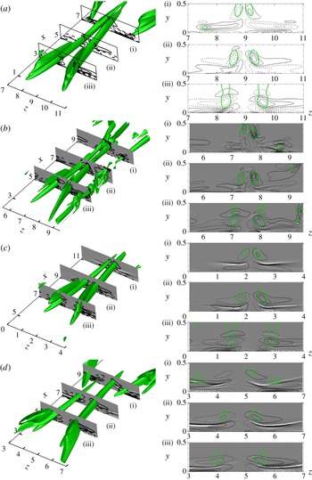
Figure 17(a) shows the results from the Newtonian case. The sign of the streamwise vorticity within the leg of the
 $\unicode[STIX]{x1D6EC}$
structure conforms to the direction of rotation, and an opposite vorticity is induced between the legs and the wall. Also the vorticity contours are concentrated within the
 $\unicode[STIX]{x1D6EC}$
-structure with similar orientation. Figure 17(b–d) show the viscoelastic cases with
 $Wi=\{1.83,4.50,6.67\}$
. The vorticity contours gradually weaken with increasing elasticity, and become less concentrated with the
 $\unicode[STIX]{x1D6EC}$
-structure. The figures are also supplemented with the perturbation polymer torque,
 $\unicode[STIX]{x1D712}_{x}^{\prime }$
, which is shown by the flood contours. The torque is primarily resistive and its sheet-like appearance (Page & Zaki Reference Page and Zaki2015) along the boundary between positive and negative vorticity is responsible for the elongation of the vorticity field in the span.
Another important observation from figure 17 is the formation of the head of the
 $\unicode[STIX]{x1D6EC}$
-structure, which is lifted away from the wall. The same tendency is noted in figure 17 for
 $Wi=4.50$
although to a lesser extent due to the slightly wider spanwise size of the structure. In both cases, however, it is anticipated that the lifted head of the vortex would roll up and generate hairpin vortices, as described by Sandham & Kleiser (Reference Sandham and Kleiser1992) for the Newtonian case. At the highest Weissenberg number, however, the spanwise size of the legs of the
 $\unicode[STIX]{x1D6EC}$
-structure are widely separated and the lifted head that is a prerequisite for roll up and final breakdown is not clear in the figure.
(Left)
 $\unicode[STIX]{x1D6EC}$
-shaped vortices for (a) Newtonian, (b)
 $Wi=1.83$
, (c)
 $Wi=4.50$
, (d)
 $Wi=6.67$
at the mid-stage of transition. (Right) End views at three downstream locations that cut through the
 $\unicode[STIX]{x1D6EC}$
-structures. Thick green line is the outline of the
 $\unicode[STIX]{x1D6EC}$
-structure; flood contours are
 $-1\leqslant \unicode[STIX]{x1D712}_{x}^{\prime }\leqslant 1$
and contour lines denote
 $\unicode[STIX]{x1D714}_{x}^{\prime }$
with spacing equal to
 $4\times 10^{-1}$
.

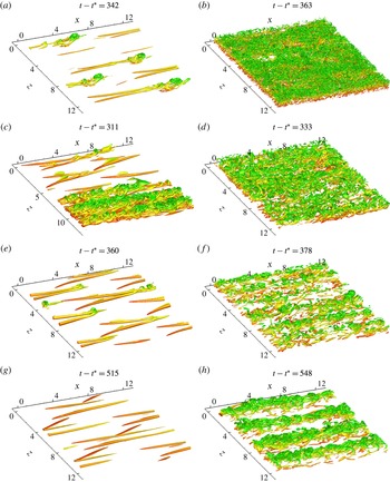
Visualization of vortical structures in (a,c,e,g) late-stage transition and (b,d,f,h) near the onset of fully turbulent flow. (a,b) Newtonian; (c,d)
 $Wi=1.83$
; (e,f)
 $Wi=4.50$
; (g,h)
 $Wi=6.67$
. The vortical structures are identified using (a,c,e,g)
 $\unicode[STIX]{x1D706}_{2}=\{-1.0,-0.2,-0.2,-0.1\}$
and (b,d,f,h)
 $\unicode[STIX]{x1D706}_{2}=\{-10.0,-2.0,-2.0,-1.0\}$
.

3.3 Late stage and breakdown to turbulence
The time shift in transition onset is mirrored by a shift in its final stage when the perturbation energy reaches a peak (figure 9). The slope of the curve
 $E(t)$
does not change appreciably among the various configurations, although the transition process requires longer time at the highest elasticity because it starts at a lower energy level.
In the final stage of transition in the Newtonian case, the spanwise vorticity at the head of the
 $\unicode[STIX]{x1D6EC}$
-structures lifts up thus forming an elevated shear layer that becomes the site of the ultimate breakdown to turbulence. This process starts by spawning an
 $\unicode[STIX]{x1D6FA}$
-shaped structure, known as a hairpin vortex. A series of hairpin vortices are further generated upstream and together form a hairpin packet (Sandham & Kleiser Reference Sandham and Kleiser1992). Figure 18 is a visualization of the vortical structures that are formed during the transition process. The Newtonian flow follows the above description, and the figure shows that the early hairpin structures spread and cover the bottom wall fully, marking the end of intermittency and the onset of the fully turbulence regime. Breakdown to turbulence in the viscoelastic flows at
 $Wi=1.83$
and
 $4.50$
are qualitatively similar. At
 $Wi=1.83$
, the hairpin packets have caused rapid breakdown to turbulence in half of the span, while transition in the rest of the domain lags slightly but ultimately becomes fully turbulent. While breakdown at
 $Wi=4.50$
most closely resembles the Newtonian case, the final state has a lower population density of vortical structures, which suggests a weaker turbulent activity and potentially lower drag.
At the highest Weissenberg number, the final stage of transition is qualitatively different from the Newtonian case. The
 $\unicode[STIX]{x1D6EC}$
-structures from the early stage continue to elongate and become progressively more aligned in the streamwise direction. Since the spanwise separation is large and the ejection event is weaker in this configuration, hairpin vortices are not formed in this case. Instead the elongated vortices and their accompanying streaks undergo secondary instability, akin to the process of streak breakdown in bypass transition (Vaughan & Zaki Reference Vaughan and Zaki2011; Hack & Zaki Reference Hack and Zaki2014). Turbulence is not spawned from localized breakdown packets, but in stripes due to the secondary instability of the entire elongated structure. Also, the strength of the vortical structures within the turbulent regime is weaker than in all the other conditions, again pointing to a weaker turbulence activity and potentially a drag-reduced turbulent state.
The evolution of transitional flow structures can be viewed as a microcosm of the dynamics in the more complex fully turbulent configurations. In a similar vein, Kim et al. (Reference Kim, Adrian, Balachandar and Sureshkumar2008) and Kim & Sureshkumar (Reference Kim and Sureshkumar2013) studied the evolution of isolated, conditionally averaged vortical structures extracted from turbulent fields. While the scales of the transitional and fully turbulent structures are different (the
 $\unicode[STIX]{x1D6EC}$
structures and the hairpin packets in our simulations are much wider than those observed in fully turbulent conditions and the mean shear distribution is different), in both configurations the polymer torque acts to oppose the vorticity perturbation, the disturbance field becomes more elongated in the streamwise direction and the hairpin packets are suppressed. These similarities are beneficial in building our understanding of the influence of elasticity on shear flows.
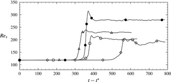
Ultimately all four simulations reach a fully turbulent state. Figure 19 shows the time evolution of the friction Reynolds number,
 $Re_{\unicode[STIX]{x1D70F}}\equiv u_{\unicode[STIX]{x1D70F}}h/\unicode[STIX]{x1D708}$
, where
 $u_{\unicode[STIX]{x1D70F}}\equiv \sqrt{\unicode[STIX]{x1D708}(\unicode[STIX]{x2202}\overline{u}/\unicode[STIX]{x2202}y)_{wall}}$
is the friction velocity evaluated from the streamwise- spanwise-averaged velocity profile. Beyond the sharp rise in
 $Re_{\unicode[STIX]{x1D70F}}$
in the transition region, it levels off to a relatively steady value in the fully turbulent regime. This plateau in
 $Re_{\unicode[STIX]{x1D70F}}$
corresponds to the saturation of the energy curves after secondary instability in figure 9.
Once the statistically stationary state was reached in each simulation, in addition to streamwise and spanwise averaging, sampling was also performed in time during
 $160$
–
 $170$
convective units. Flow quantities are then decomposed as
 $\unicode[STIX]{x1D703}=\langle \unicode[STIX]{x1D703}\rangle +\unicode[STIX]{x1D703}^{\prime }$
, where the angle brackets denote the steady mean. The friction velocity of the fully turbulent stage is therefore
 $u_{\langle \unicode[STIX]{x1D70F}\rangle }\equiv \sqrt{\unicode[STIX]{x1D708}(\text{d}\langle u\rangle /\text{d}y)_{wall}}$
; the corresponding friction Reynolds numbers are
 $Re_{\langle \unicode[STIX]{x1D70F}\rangle }\equiv u_{\langle \unicode[STIX]{x1D70F}\rangle }h/\unicode[STIX]{x1D708}=\{278,230,202,187\}$
for the Newtonian and three viscoelastic cases with increasing
 $Wi$
. A lower drag state is established in the viscoelastic flows relative to the Newtonian case, even at
 $Wi=1.83$
which is more unstable and breaks down to turbulence fastest. The reduction in the turbulent drag is more pronounced at higher elasticity. Expressed in terms of the change in
 $\langle Re_{\unicode[STIX]{x1D70F}}\rangle$
, drag reduction is defined as,
 $$\begin{eqnarray}DR\equiv \frac{u_{\langle \unicode[STIX]{x1D70F}\rangle ,N}^{2}-u_{\langle \unicode[STIX]{x1D70F}\rangle }^{2}}{u_{\langle \unicode[STIX]{x1D70F}\rangle ,N}^{2}}=\left[1-\left(\frac{Re_{\langle \unicode[STIX]{x1D70F}\rangle }}{Re_{\langle \unicode[STIX]{x1D70F}\rangle ,N}}\right)^{2}\right],\end{eqnarray}$$
where subscript ‘
 $N$
’ marks the Newtonian value. For
 $Wi=1.83,4.50$
and
 $6.67$
, the drag reduction is 31.5 %, 47.2 % and 54.7 %. The viscoelastic flows are therefore in the low-, intermediate- and high-drag-reduction regimes, in comparison to the maximum drag-reduction (MDR) state where
 $DR\approx 70\,\%$
(Warholic, Massah & Hanratty Reference Warholic, Massah and Hanratty1999).
Time evolution of the friction Reynolds number,
 $Re_{\unicode[STIX]{x1D70F}}$
, beyond the addition of background white disturbances at
 $t-t^{\ast }=0$
. (—●—) Newtonian; (—▵—)
 $Wi=1.83$
; (—○—)
 $Wi=4.50$
; (—♢—)
 $Wi=6.67$
.

Statistics from fully turbulent state at
 $Re=4667$
,
 $\unicode[STIX]{x1D6FD}=0.9$
and
 $L_{max}=100$
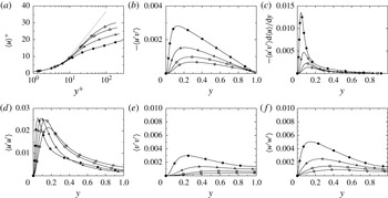
. (a) Mean velocity profiles in wall units and the Virk MDR asymptote in grey; (b) Reynolds shear stress; (c) production of streamwise velocity perturbation; (d–f) Reynolds normal stresses. The lines correspond to the four conditions: (—●—) Newtonian; (—▵—)
 $Wi=1.83$
; (—○—)
 $Wi=4.50$
; (—♢—)
 $Wi=6.67$
.

The mean velocity profile, the Reynolds stresses and turbulence production are plotted in figure 20. As elasticity increases, the mean velocity profile progressively approaches the Virk asymptote, which marks the MDR state (Virk & Mickley Reference Virk and Mickley1970). The peak in the Reynolds streamwise stress,
 $\langle u^{\prime }u^{\prime }\rangle$
, shifts away from the wall, and becomes observably weaker at
 $Wi=6.67$
. Since
 $\langle u^{\prime }u^{\prime }\rangle$
is predominantly due to the streaks, its peak location is determined by the lift-up process, which is encapsulated in the production term,
 $-\langle u^{\prime }v^{\prime }\rangle \text{d}\langle u\rangle /\text{d}y$
. In the Newtonian case, the mean shear is localized in the near-wall region, thus drawing the peak production and
 $\langle u^{\prime }u^{\prime }\rangle$
closer to the wall than in the viscoelastic conditions. It should also be noted that, if normalized by the friction velocity, the streamwise stress appears to increase with elasticity due to the appreciable decrease in
 $u_{\unicode[STIX]{x1D70F}}$
in the drag-reduced state. This trend is consistent with earlier studies of polymer drag reduction (Dimitropoulos, Sureshkumar & Beris Reference Dimitropoulos, Sureshkumar and Beris1998; Warholic et al.
Reference Warholic, Massah and Hanratty1999; Dubief et al.
Reference Dubief, White, Terrapon, Shaqfeh, Moin and Lele2004; Dimitropoulos et al.
Reference Dimitropoulos, Dubief, Shaqfeh, Moin and Lele2005). On the other hand, the cross-flow components,
 $\langle v^{\prime }v^{\prime }\rangle$
and
 $\langle w^{\prime }w^{\prime }\rangle$
, are appreciably suppressed whether scaled by outer or inner units. Their significant attenuation with increasing
 $Wi$
is consistent with viscoelasticity effectively weakening streamwise vortical motions that lead to the amplification of streaks.
4 Conclusion
Breakdown to turbulence in channel flow is generally classified as either orderly or bypass transition. Previous numerical studies have examined the latter route in detail for both Newtonian and polymeric flows. On the other hand, simulations of orderly transition have only been performed for Newtonian conditions. In the present work, direct numerical simulations were performed to examine orderly transition in polymeric channel flow, starting from the amplification of primary Tollmien–Schlichting waves, their secondary instability and ultimately full nonlinear breakdown to turbulence.
Three Weissenberg numbers were selected for this study and were compared to a reference Newtonian case. The Reynolds number in all simulations was
 $Re=4667$
, which is supercritical. The choice of the Weissenberg number was motivated by results from linear stability theory: at a prescribed Reynolds number, the primary Tollmien–Schlichting wave initially becomes more unstable with elasticity and is subsequently stabilized at higher
 $Wi$
. The lowest elasticity condition was
 $Wi=1.83$
, which corresponds to the highest growth rate of the primary TS wave at
 $Re=4667$
. The intermediate elasticity was
 $Wi=4.50$
, where the growth rate of the primary TS wave matches the Newtonian value. Finally,
 $Wi=6.67$
in the stabilized regime where the growth of the primary TS wave is slower than Newtonian.
Beyond the early linear regime, and in the absence of additional background disturbances, the Tollmien–Schlichting wave reaches a saturated state in the Newtonian case. This marks a state where the energy extracted from the distorted base flow equals the dissipation by the saturated instability. The same behaviour is observed in the low and high Weissenberg number cases, even though the governing equations are supplemented by the polymer work term. At
 $Wi=4.50$
, however, a saturated state was not reached. These nonlinear simulations also demonstrated that the maximum possible amplitude of a saturated TS wave decreases with increasing elasticity (e.g.
 $u_{max}^{\prime }=1.6\,\%$
of the mean flow at saturation when
 $Wi=6.67$
). As such, these simulations are a prerequisite for defining a feasible initial condition for transition simulations; it is not physical to start from a linear mode with amplitude of the order of
 $3\,\%$
of the mean flow as customary in simulations of natural transition in Newtonian flows.
An initial nonlinear state was extracted and broadband white noise was added to the velocity field in order to trigger the onset of secondary instability. In all cases, the flow underwent secondary instability and ultimately breakdown to turbulence. Compared to the Newtonian case, the onset of the secondary instability is at higher energy level for the destabilized low elasticity flow, and at lower energy for the stabilized higher
 $Wi$
cases. Of the total energy, the largest fraction is maintained within the streamwise component of velocity.
While all conditions show the emergence of three-dimensional
 $\unicode[STIX]{x1D6EC}$
-structures during the secondary instability stage, the spanwise wavenumbers of the instabilities differ. Relative to the Newtonian case, a narrower spacing is observed at
 $Wi=1.83$
and wider for
 $Wi=6.67$
. The latter configuration is accompanied by a weaker ejection between the legs of the
 $\unicode[STIX]{x1D6EC}$
-structures and, as such, weaker low-speed streaks. Subsequently, all but the highest Weissenberg number case undergo breakdown via the generation of hairpin packets due to the lifted head of the
 $\unicode[STIX]{x1D6EC}$
-structure. For
 $Wi=6.67$
, however, the lack of a strong ejection event disallows this mechanism. Instead, the vortical structures become very long in the streamwise direction and break down to turbulence in a manner similar to streaks in bypass transition.
The ultimate state from all four simulations is fully turbulent flow. Independent of the influence of elasticity, be it destabilizing at
 $Wi=1.83$
or stabilizing at the higher Weissenberg numbers, the turbulent flow reaches a reduced-drag state in all three polymeric conditions. The extent of drag reduction increased with elasticity, with the mean profile progressively approaching the Virk asymptote.
The present simulations demonstrate that elasticity affects not only the linear growth of Tollmien–Schlichting waves and the ultimate turbulent state that emerges at the end of transition, but also the secondary instability. The results thus complement existing studies of linear instability waves in polymeric fluids and the nonlinear simulations and experiments of bypass transition and turbulent drag-reduced flows.
Acknowledgements
The authors thank Dr J. Page for providing the linear stability algorithm, and Dr A. Agarwal and I. Hameduddin for assisting in the validation of the simulations. This work is sponsored by the National Science Foundation under grant no. 1511937.
Appendix A. Linear stability equations
The linear stability equations for laminar channel flow of a FENE-P fluid are provided in this appendix. The starting point is to decompose the total velocity and conformation tensor into a base state and a perturbation,
 $u_{i}=U_{i}+u_{i}^{\prime }$
and
 $\unicode[STIX]{x1D624}_{ij}=\unicode[STIX]{x1D60A}_{ij}+\unicode[STIX]{x1D624}_{ij}^{\prime }$
. The linearized equations governing the evolution of the perturbations are,
 $$\begin{eqnarray}\displaystyle & \displaystyle \frac{\unicode[STIX]{x2202}u_{j}^{\prime }}{\unicode[STIX]{x2202}x_{j}}=0, & \displaystyle\end{eqnarray}$$
 $$\begin{eqnarray}\displaystyle & \displaystyle \left(\frac{\unicode[STIX]{x2202}u_{i}^{\prime }}{\unicode[STIX]{x2202}t}+U_{j}\frac{\unicode[STIX]{x2202}u_{i}^{\prime }}{\unicode[STIX]{x2202}x_{j}}+u_{j}^{\prime }\frac{\unicode[STIX]{x2202}U_{i}}{\unicode[STIX]{x2202}x_{j}}\right)=-\frac{\unicode[STIX]{x2202}p^{\prime }}{\unicode[STIX]{x2202}x_{i}}+\frac{\unicode[STIX]{x1D6FD}}{Re}\frac{\unicode[STIX]{x2202}^{2}u_{i}^{\prime }}{\unicode[STIX]{x2202}x_{j}\unicode[STIX]{x2202}x_{j}}+\frac{(1-\unicode[STIX]{x1D6FD})}{Re}\frac{\unicode[STIX]{x2202}\unicode[STIX]{x1D749}_{ij}^{\prime }}{\unicode[STIX]{x2202}x_{j}}, & \displaystyle\end{eqnarray}$$
 $$\begin{eqnarray}\displaystyle & \displaystyle \frac{\unicode[STIX]{x2202}\unicode[STIX]{x1D624}_{ij}^{\prime }}{\unicode[STIX]{x2202}t}+U_{k}\frac{\unicode[STIX]{x2202}\unicode[STIX]{x1D624}_{ij}^{\prime }}{\unicode[STIX]{x2202}x_{k}}+u_{k}^{\prime }\frac{\unicode[STIX]{x2202}\unicode[STIX]{x1D60A}_{ij}}{\unicode[STIX]{x2202}x_{k}}=\unicode[STIX]{x1D60A}_{ik}\frac{\unicode[STIX]{x2202}u_{j}^{\prime }}{\unicode[STIX]{x2202}x_{k}}+\unicode[STIX]{x1D624}_{ik}^{\prime }\frac{\unicode[STIX]{x2202}U_{j}}{\unicode[STIX]{x2202}x_{k}}+\unicode[STIX]{x1D60A}_{kj}\frac{\unicode[STIX]{x2202}u_{i}^{\prime }}{\unicode[STIX]{x2202}x_{k}}+\unicode[STIX]{x1D624}_{kj}^{\prime }\frac{\unicode[STIX]{x2202}U_{i}}{\unicode[STIX]{x2202}x_{k}}-\unicode[STIX]{x1D749}_{ij}^{\prime }. & \displaystyle\end{eqnarray}$$
 $\unicode[STIX]{x1D749}_{ij}^{\prime }$
, is derived from (2.3) by performing a Taylor series expansion of
 $1/\unicode[STIX]{x1D713}$
, and retaining terms up to
 $O(\unicode[STIX]{x1D624}_{ij}^{\prime })$
only,
 $$\begin{eqnarray}\displaystyle \unicode[STIX]{x1D749}_{ij}^{\prime }=\frac{1}{Wi}\left(1-\frac{\unicode[STIX]{x1D60A}_{kk}}{L_{max}^{2}}\right)^{-1}\left(\unicode[STIX]{x1D624}_{ij}^{\prime }+\frac{\unicode[STIX]{x1D60A}_{ij}\unicode[STIX]{x1D624}_{kk}^{\prime }}{L_{max}^{2}-\unicode[STIX]{x1D60A}_{kk}}\right). & & \displaystyle\end{eqnarray}$$
Assuming a parallel base flow profile along with the associated base state stresses (2.10)–(2.12), a normal modes expansion may be adopted for the perturbation field,
 $$\begin{eqnarray}\unicode[STIX]{x1D719}^{\prime }(\boldsymbol{x},t)=\tilde{\unicode[STIX]{x1D719}}(y)\exp [\text{i}(k_{x}x+k_{z}z-\unicode[STIX]{x1D70E}t)].\end{eqnarray}$$
The focus of the present study is on two-dimensional disturbances, hence the spanwise wavenumber is set to zero,
 $k_{z}=0$
. The linear system (A 1) reduces to,
 $$\begin{eqnarray}\displaystyle & \displaystyle \text{i}k_{x}\tilde{u} +\frac{\text{d}\tilde{v}}{\text{d}y}=0, & \displaystyle\end{eqnarray}$$
 $$\begin{eqnarray}\displaystyle & \displaystyle (-\text{i}\unicode[STIX]{x1D70E}+\text{i}k_{x}U)\tilde{u} +\tilde{v}\frac{\text{d}U}{\text{d}y}=-\text{i}k_{x}\tilde{p}+\frac{\unicode[STIX]{x1D6FD}}{Re}\!\left(\frac{\text{d}^{2}}{\text{d}y^{2}}-k_{x}^{2}\right)\tilde{u} +\frac{(1-\unicode[STIX]{x1D6FD})}{Re}\!\left(\text{i}k_{x}\tilde{\unicode[STIX]{x1D749}}_{xx}+\frac{\text{d}\tilde{\unicode[STIX]{x1D749}}_{xy}}{\text{d}y}\right)\!, & \displaystyle\end{eqnarray}$$
 $$\begin{eqnarray}\displaystyle & \displaystyle (-\text{i}\unicode[STIX]{x1D70E}+\text{i}k_{x}U)\tilde{v}=-\frac{\text{d}\tilde{p}}{\text{d}y}+\frac{\unicode[STIX]{x1D6FD}}{Re}\left(\frac{\text{d}^{2}}{\text{d}y^{2}}-k_{x}^{2}\right)\tilde{v}+\frac{(1-\unicode[STIX]{x1D6FD})}{Re}\left(\text{i}k_{x}\tilde{\unicode[STIX]{x1D749}}_{xy}+\frac{\text{d}\tilde{\unicode[STIX]{x1D749}}_{yy}}{\text{d}y}\right), & \displaystyle\end{eqnarray}$$
 $$\begin{eqnarray}\displaystyle & \displaystyle (-\text{i}\unicode[STIX]{x1D70E}+\text{i}k_{x}U)\tilde{\unicode[STIX]{x1D624}}_{xx}+\tilde{v}\frac{\text{d}\unicode[STIX]{x1D60A}_{xx}}{\text{d}y}+\tilde{\unicode[STIX]{x1D749}}_{xx}=2\text{i}k_{x}\unicode[STIX]{x1D60A}_{xx}\tilde{u} +2\unicode[STIX]{x1D60A}_{xy}\frac{\text{d}\tilde{u} }{\text{d}y}+2\frac{\text{d}U}{\text{d}y}\tilde{\unicode[STIX]{x1D624}}_{xy}, & \displaystyle\end{eqnarray}$$
 $$\begin{eqnarray}\displaystyle & \displaystyle (-\text{i}\unicode[STIX]{x1D70E}+\text{i}k_{x}U)\tilde{\unicode[STIX]{x1D624}}_{xy}+\tilde{v}\frac{\text{d}\unicode[STIX]{x1D60A}_{xy}}{\text{d}y}+\tilde{\unicode[STIX]{x1D749}}_{xy}=\text{i}k_{x}\unicode[STIX]{x1D60A}_{xx}\tilde{v}+\unicode[STIX]{x1D60A}_{yy}\frac{\text{d}\tilde{u} }{\text{d}y}+\frac{\text{d}U}{\text{d}y}\tilde{\unicode[STIX]{x1D624}}_{yy}, & \displaystyle\end{eqnarray}$$
 $$\begin{eqnarray}\displaystyle & \displaystyle (-\text{i}\unicode[STIX]{x1D70E}+\text{i}k_{x}U)\tilde{\unicode[STIX]{x1D624}}_{yy}+\tilde{v}\frac{\text{d}\unicode[STIX]{x1D60A}_{yy}}{\text{d}y}+\tilde{\unicode[STIX]{x1D749}}_{yy}=2\text{i}k_{x}\unicode[STIX]{x1D60A}_{xy}\tilde{v}+2\unicode[STIX]{x1D60A}_{yy}\frac{\text{d}\tilde{v}}{\text{d}y}, & \displaystyle\end{eqnarray}$$
 $$\begin{eqnarray}\displaystyle & \displaystyle (-\text{i}\unicode[STIX]{x1D70E}+\text{i}k_{x}U)\tilde{\unicode[STIX]{x1D624}}_{zz}+\tilde{\unicode[STIX]{x1D749}}_{zz}=0. & \displaystyle\end{eqnarray}$$
 $\unicode[STIX]{x1D70E}$
. The eigenvalue problem (A 4) is discretized using a Chebyshev polynomial expansion in the wall-normal direction along Gauss–Lobatto collocation points. Typically
 $N=128$
polynomials are required to accurately resolve the TS waves. For each axial wavenumber and Reynolds and Weissenberg number pair, a spectrum of eigenmodes is obtained. The most unstable mode is then extracted, and corresponds to the complex frequency with the largest imaginary part,
 $\unicode[STIX]{x1D70E}_{i}$
.