1 Introduction
1.1 The broader context
Surface wave breaking plays an important role in the coupling between the atmosphere and the ocean from local weather to global climate scales. In the absence of wave breaking, the direct transport between the atmosphere and the ocean is through slow molecular diffusion and conduction processes. In contrast, when a wave breaks, the surface may experience dramatic changes, with a jet forming and plunging back to the surface, ejecting spray and entraining air into the ocean. For weaker breaking, the surface may roll over itself down the front of the wave while still entraining bubbles.
Breaking is a transitional flow process from the laminar fluid dynamics of classical surface waves to a two-phase turbulent flow. Thus wave breaking limits the height of surface waves, transfers momentum from waves to currents and significantly enhances the transfer of heat, water vapour, marine aerosols and gases between the atmosphere and the ocean (Memery & Merlivat Reference Memery and Merlivat1985; Farmer, McNeil & Johnson Reference Farmer, McNeil and Johnson1993; Melville Reference Melville1996). Approximately 30 % of the
 $\text{CO}_{2}$
released into the atmosphere is taken up by the ocean (Rhein et al.
Reference Rhein, Rintoul, Aoki, Campos, Chambers, Feely, Gulev, Johnson, Josey, Kostianoy, Stocker, Qin, Plattner, Tignor, Allen, Boschung, Nauels, Xia, Bex and Midgley2013), much from the entrainment and dissolution of bubbles by breaking and the associated mixing (Monahan & Dam Reference Monahan and Dam2001). Once in solution,
 $\text{CO}_{2}$
forms carbonic acid, the source of ocean acidification, which has such an adverse effect on shell-forming marine animals. Breaking impact forms spray and aerosols, while small bubbles may be dissolved into the water column, larger bubbles entrained by breaking rise back to the surface and collapse. This generates spray, which is transported into the atmosphere and ultimately evaporates leaving water vapour, important for the thermodynamics of the atmosphere, and salt crystals that affect the radiative balance of the atmosphere and form cloud condensation nuclei (Andreas et al.
Reference Andreas, Edson, Monahan, Rouault and Smith1995; de Leeuw et al.
Reference de Leeuw, Andreas, Anguelova, Fairall, Lewis, O’Dowd, Schulz and Schwartz2011; Veron Reference Veron2015).
For all these reasons, improvement in our understanding of the ocean, atmosphere and climate systems require a detailed understanding of the physics of air entrainment and subsequent bubble generation. Due to the complex nature of the breaking process, a coupled two-phase turbulent flow, a detailed understanding of the dynamical and statistical properties of the generated bubbles has been elusive.
1.2 Bubble size distribution, models and observations
The bubble size distribution is the most important characteristic of the bubble formation process since one can retrieve the bubble cloud properties, volume, energy and penetration depth from its moments. Garrett, Li & Farmer (Reference Garrett, Li and Farmer2000) introduced the most widely used model for the bubble size distribution. It relies on a steady model of a turbulent break-up cascade, assuming the size distribution per unit volume
 $\mathscr{N}(r)$
, with
 $r$
the bubble radius, to depend only on the local (time-averaged) turbulent dissipation rate
 $\bar{{\it\varepsilon}}$
, the bubble radius
 $r$
and the source of bubbles, i.e. the constant air flow rate per unit volume of water
 $Q$
. The steady assumption requires
 $\mathscr{N}(r)\propto Q$
, then dimensional analysis leads to
 $$\begin{eqnarray}\mathscr{N}(r)\propto Q\bar{{\it\varepsilon}}^{-1/3}r^{-10/3}.\end{eqnarray}$$
Note that Garrett et al. (Reference Garrett, Li and Farmer2000) consider the bubble size distribution per unit volume
 $\mathscr{N}(r)$
, which is physically equivalent to
 $N(r)$
, the bubble size distribution (
 $\mathscr{N}(r)\,\text{d}r$
and
 $N(r)\,\text{d}r$
are respectively the per unit volume, and absolute number of bubbles of radii between
 $r$
and
 $r+\text{d}r$
). If one considers
 $N(r)$
, (1.1) is unchanged, except
 $Q$
is now the absolute air flow rate.
The related turbulent break-up model assumes an inertial subrange and a direct cascade process: air is injected at large scales (large bubbles) by the entrainment process and turbulent fluctuations break them into smaller bubbles. The cascade process ends at the scale where surface tension prevents further bubble break-up, the Hinze scale (Hinze Reference Hinze1955):
 $$\begin{eqnarray}r_{H}=\mathscr{C}({\it\gamma}/{\it\rho})^{3/5}\bar{{\it\varepsilon}}^{-2/5},\end{eqnarray}$$
where
 ${\it\gamma}$
is the surface tension,
 ${\it\rho}$
the water density and
 $\mathscr{C}$
is a dimensionless constant which has a value of approximately 0.5 (Martinez-Bazan, Montanes & Lasheras Reference Martinez-Bazan, Montanes and Lasheras1999; Garrett et al.
Reference Garrett, Li and Farmer2000; Deane & Stokes Reference Deane and Stokes2002).
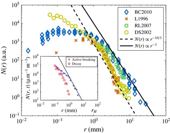
Bubble size distributions
 $N(r)$
, measured during various breaking-wave laboratory experiments in the existing literature. Dashed line is
 $N(r)\propto r^{-10/3}$
and solid line is
 $N(r)\propto r^{-3}$
. Size distributions are given in arbitrary units due to various normalizations in the original papers. (♢) BC2010 stands for Blenkinsopp & Chaplin (Reference Blenkinsopp and Chaplin2010), (
 $\times$
) L1996 for Loewen, O’Dor & Skafel (Reference Loewen, O’Dor and Skafel1996), (▫) RL2007 for Rojas & Loewen (Reference Rojas and Loewen2007) and (○) DS2002 for Deane & Stokes (Reference Deane and Stokes2002). (Inset) Experimental bubble size distributions
 $N(r,t)$
from Deane & Stokes (Reference Deane and Stokes2002), during the active breaking stage (
 $+$
) and later during the decay (○). Solid line is
 $N(r,t)\propto r^{-3}$
.
 $N(r,t)$
is much steeper once the active breaking stage is finished.

Several experimental studies (Loewen et al.
Reference Loewen, O’Dor and Skafel1996; Terrill, Melville & Stramski Reference Terrill, Melville and Stramski2001; Deane & Stokes Reference Deane and Stokes2002; Leifer & de Leeuw Reference Leifer and de Leeuw2006; Rojas & Loewen Reference Rojas and Loewen2007; Blenkinsopp & Chaplin Reference Blenkinsopp and Chaplin2010) have identified a bubble size distribution following a power law of the bubble radius
 $N(r)\propto r^{-m}$
with
 $m\in [2.5:3.5]$
, roughly compatible with (1.1) when considering the difficulty of the experiments. Figure 1 shows the bubble size distribution from various laboratory studies, using different measurement methods: cameras and bubble interface detection technique (Deane & Stokes Reference Deane and Stokes2002), fiber optical probes (Rojas & Loewen Reference Rojas and Loewen2007; Blenkinsopp & Chaplin Reference Blenkinsopp and Chaplin2010) or acoustic instruments (Loewen et al.
Reference Loewen, O’Dor and Skafel1996). From figure 1 it is hard to make a clear statement on the exact value of the power-law exponent
 $m$
. Data from Loewen et al. (Reference Loewen, O’Dor and Skafel1996) and Deane & Stokes (Reference Deane and Stokes2002) are closer to the
 $m=10/3$
value while data from more recent experiments show values closer to
 $m=3$
(Rojas & Loewen Reference Rojas and Loewen2007; Blenkinsopp & Chaplin Reference Blenkinsopp and Chaplin2010). Moreover, the experiments by Deane & Stokes (Reference Deane and Stokes2002) and Blenkinsopp & Chaplin (Reference Blenkinsopp and Chaplin2010) give very different shapes for
 $N(r)$
below the Hinze scale.
One of the difficulties in properly identifying the exponent
 $m$
is the rapid time variations of the bubble size distribution. As discussed by Deane & Stokes (Reference Deane and Stokes2002) and shown in figure 1 (inset), the scaling
 $N(r)\propto r^{-m}$
, with
 $m\in [2.5:3.5]$
, is only valid during the active breaking time, which is approximately one wave period. Later on, the bubble size distribution is found to be much steeper. Therefore, it is possible that the different values for
 $m$
found in the literature are related to the time of observation and the time of averaging used to calculate
 $N(r)$
. Therefore, a more complete description of the time evolution of the bubble size distribution during the breaking event and during the rise of the bubbles is needed.
Indeed, the model from Garrett et al. (Reference Garrett, Li and Farmer2000) (1.1), while undoubtedly correct for constant
 $Q$
, does not describe the temporal evolution in which the bubble size distribution experiences very rapid change (Terrill et al.
Reference Terrill, Melville and Stramski2001; Deane & Stokes Reference Deane and Stokes2002). Moreover, measurements of the volume of entrained air have shown that
 $Q$
is not a constant parameter in this problem (Lamarre & Melville Reference Lamarre and Melville1991; Blenkinsopp & Chaplin Reference Blenkinsopp and Chaplin2007). Finally the dependence on
 $\bar{{\it\varepsilon}}$
and
 $Q$
in (1.1) has never been validated and raises a concern. In breaking waves, even if there were a constant
 $Q$
for some time, it would almost certainly depend on
 $\bar{{\it\varepsilon}}$
, in which case we might expect that
 $Q\bar{{\it\varepsilon}}^{-1/3}\propto \bar{{\it\varepsilon}}^{n}$
, with
 $n>0$
. Thus, understanding the link between these two variables is crucial and will clarify the relationship between the kinematics and dynamics of the flow (e.g. dissipation, air entrainment rate) and the integral quantities, through the moments of the size distribution.
Baldy (Reference Baldy1993) proposed another model for bubble generation by breaking waves, also based on a turbulent break-up scenario, which describes
 $s(r,t)$
the bubble size distribution per unit time, per unit mass per unit ocean surface area, assuming adiabatic evolution, i.e. the time scale of bubble fragmentation is much faster than the other processes at play. Considering that
 $s(r,t)$
is given by the balance of the local time-dependent turbulent dissipation rate
 ${\it\varepsilon}(t)$
and characteristic surface tension energy of a single bubble
 $e_{s}\propto {\it\gamma}r^{2}/{\it\rho}$
, Baldy (Reference Baldy1993) found by dimensional analysis:
 $$\begin{eqnarray}s(r,t)\propto \frac{{\it\varepsilon}(t)}{({\it\gamma}/{\it\rho})r^{2}}\propto {\it\varepsilon}(t)\left(\frac{{\it\gamma}}{{\it\rho}}\right)^{-1}r^{-2}.\end{eqnarray}$$
This model is appealing because it considers only the bubble energy and the turbulent break-up dissipation rate while Garrett et al. (Reference Garrett, Li and Farmer2000) had to introduce the constant air flow rate
 $Q$
to close their dimensional argument. Since this model is adiabatic in time, the measurable time-averaged bubble size distribution
 $N(r)$
is going to be
 $N(r)\propto r^{-2}$
. However, as discussed before, experimental results suggest that
 $N(r)\propto r^{-m}$
, with
 $m\in [2.5:3.5]$
, which is quite different from the above result (1.3). Note also that this model is based on an inertial subrange hypothesis without indications of the scale of the smallest bubble, so the role of the Hinze scale in this description is therefore not clear.
On the other hand, the Garrett et al. (Reference Garrett, Li and Farmer2000) model predicts
 $m=10/3$
, which, within the scatter, is in agreement with experimental data. An important difference between the models from Baldy (Reference Baldy1993) and Garrett et al. (Reference Garrett, Li and Farmer2000) concerns the treatment of surface tension. Baldy (Reference Baldy1993) considers surface tension energy as the key parameter to balance the turbulent break-up of the bubbles within the turbulent inertial subrange, while Garrett et al. (Reference Garrett, Li and Farmer2000) neglect surface tension for bubbles of radius larger than the Hinze scale, assuming that surface tension is the process that stops the turbulent break-up at small scales.
1.3 Numerical simulations
Besides laboratory and field work, numerical simulations of two-phase breaking wave flow have recently become available through improvements in numerical schemes and increases in computational capacity, but they remain very challenging. Two approaches exist: large eddy simulations (LES), with subgrid-scale turbulent and bubbly flow models and direct numerical simulations (DNS). While LES solves the large scales directly, strong assumptions are needed for the subgrid-scale turbulent bubbly flow closures, e.g. by assuming a bubble size distribution (Shi, Kirby & Ma Reference Shi, Kirby and Ma2010; Liang et al. Reference Liang, McWilliams, Sullivan and Baschek2011, Reference Liang, McWilliams, Sullivan and Baschek2012; Derakhti & Kirby Reference Derakhti and Kirby2014). In contrast, DNS is an appealing tool since no parametrizations are used to solve the multiphase flow. DNS has been limited to two-dimensional evolution of periodic unstable waves with relatively small wavelengths, and has provided numerical data on wave dissipation and splashing processes (Chen et al. Reference Chen, Kharif, Zaleski and Li1999; Song & Sirviente Reference Song and Sirviente2004; Iafrati Reference Iafrati2011; Deike, Popinet & Melville Reference Deike, Popinet and Melville2015). Three-dimensional simulations of breaking waves have recently become available through both DNS (Fuster et al. Reference Fuster, Agbaglah, Josserand, Popinet and Zaleski2009) and LES (Derakhti & Kirby Reference Derakhti and Kirby2014; Lubin & Glockner Reference Lubin and Glockner2015). They are indeed necessary to investigate bubble and spray formation, which are fundamentally three-dimensional processes. We present here a DNS study of air entrainment and the bubble statistics in three-dimensional breaking waves, for various breaking intensities. The focus is on air entrainment while predictions of spray formation will be considered in future work.
1.4 Outline
We present novel DNS of the two-phase air–water flow permitting solutions for fully three-dimensional breaking waves including air entrainment and subsequent bubble formation. We investigate both the time evolution of the air entrainment, through the total volume of entrained air, the void fraction and the evolution of the bubble size distribution together with the dependence of these quantities on the turbulent dissipation rate and the initial wave slope. The results are based on ensemble-averaged simulations, allowing a better resolution of the statistical properties of the bubbly flow.
The paper is organized as follows. Section 2 presents the numerical experiment and § 3 the numerical results for both the time-dependent and time-averaged variables of the problem. Section 4 presents an alternative phenomenological model, based on the idea that during the breaking and air entrainment processes the mechanical dissipation scales with the work done against buoyancy forces. Our model is compatible with existing experimental and DNS results, both for the time-dependent and time-averaged bubble size distribution. Finally, this model is tested against available laboratory data and our numerical data and applied to scale the integral quantities of the flow in § 5. Conclusions are presented in § 6.
2 Numerical experiments
2.1 The Gerris flow solver
We solve the three-dimensional two-phase incompressible Navier–Stokes equations accounting for surface tension and viscous effects using the open source solver Gerris (Popinet Reference Popinet2003, Reference Popinet2009), based on a quad/octree adaptive spatial discretization, multilevel Poisson solver. The interface between the high density liquid (water) and the low density gas (air) is reconstructed by a geometric volume of fluid (VOF) method. The multifluid interface is traced by a function
 $\mathscr{T}(\boldsymbol{x},t)$
, defined as the volume fraction of a given fluid in each cell of the computational mesh. The density and viscosity can thus be written as
 ${\it\rho}(\mathscr{T})=\mathscr{T}{\it\rho}_{w}+(1-\mathscr{T}){\it\rho}_{a}$
,
 ${\it\mu}(\mathscr{T})=\mathscr{T}{\it\mu}_{w}+(1-\mathscr{T}){\it\mu}_{a}$
, with
 ${\it\rho}_{w}$
,
 ${\it\rho}_{a}$
and
 ${\it\mu}_{w}$
,
 ${\it\mu}_{a}$
the density and viscosity of the two fluids (water and air), respectively. The incompressible, variable density, Navier–Stokes equations with surface tension can be written as
 $$\begin{eqnarray}\left.\begin{array}{@{}c@{}}\displaystyle {\it\rho}(\partial _{t}\boldsymbol{u}+(\boldsymbol{u}\boldsymbol{\cdot }\boldsymbol{{\rm\nabla}})\boldsymbol{u})=-\boldsymbol{{\rm\nabla}}p+\boldsymbol{{\rm\nabla}}\boldsymbol{\cdot }(2{\it\mu}\boldsymbol{D})+\displaystyle {\it\gamma}{\it\kappa}{\it\delta}_{s}\boldsymbol{n}\\ \displaystyle \partial _{t}{\it\rho}+\boldsymbol{{\rm\nabla}}\boldsymbol{\cdot }({\it\rho}\boldsymbol{u})=0\\ \boldsymbol{{\rm\nabla}}\boldsymbol{\cdot }\boldsymbol{u}=0,\end{array}\right\}\end{eqnarray}$$
with
 $\boldsymbol{u}=(u,v,w)$
the fluid velocity,
 ${\it\rho}\equiv {\it\rho}(\boldsymbol{x},t)$
the fluid density,
 ${\it\mu}\equiv {\it\mu}(\boldsymbol{x},t)$
the dynamic viscosity and
 $\boldsymbol{D}$
the deformation tensor defined as
 $\boldsymbol{D}_{ij}\equiv (\partial _{i}u_{j}+\partial _{j}u_{i})/2$
. The Dirac delta,
 ${\it\delta}_{s}$
, expresses the fact that the surface tension term is concentrated on the interface, where
 ${\it\gamma}$
is the surface tension coefficient,
 ${\it\kappa}$
and
 $\boldsymbol{n}$
the curvature and normal to the interface.
This solver has been successfully used in multiphase problems such as atomization (Fuster et al. Reference Fuster, Agbaglah, Josserand, Popinet and Zaleski2009; Agbaglah et al. Reference Agbaglah, Delaux, Fuster, Hoepffner, Josserand, Popinet, Ray, Scardovelli and Zaleski2011; Chen et al. Reference Chen, Ma, Yang and Popinet2013), the growth of instabilities at the interface (Fuster et al. Reference Fuster, Matas, Marty, Popinet, Hoepffner, Cartellier and Zaleski2013), wave breaking in two (Deike et al. Reference Deike, Popinet and Melville2015) and three dimensions (Fuster et al. Reference Fuster, Agbaglah, Josserand, Popinet and Zaleski2009), capillary wave turbulence (Deike et al. Reference Deike, Fuster, Berhanu and Falcon2014) and splashing (Thoraval et al. Reference Thoraval, Takehara, Etoh, Popinet, Ray, Josserand, Zaleski and Thoroddsen2012).
2.2 Interface reconstruction and bubble counting
In Gerris, the interface between volumes of water (tracer
 $\mathscr{T}=1$
) and air (tracer
 $\mathscr{T}=0$
) is reconstructed by a discrete geometric VOF method (Scardovelli & Zaleski Reference Scardovelli and Zaleski1999). In the geometric VOF formulation, the volume fraction field is the exact integral of the volume fraction in each discretisation element. It is not ‘smeared’ or ‘diffused’, i.e. the volume fraction is one or zero in cells which do not contain an interface and between zero and one in cells which contain an interface. The interface can then be reconstructed unambiguously in each cell with second-order accuracy (using piecewise-linear elements). These reconstructed piecewise-linear elements are displayed graphically in figures 2–4. These images are thus directly representative of the accuracy of the interface representation by the VOF method.
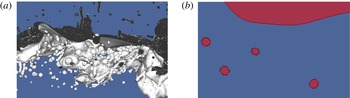
(a) Example of the VOF interface after wave breaking, with numerous visible bubbles in water and droplets in the air. (b) Zoom and cut through the vertical plane, orthogonal to the transverse direction, of (a), showing the principle of the bubble (and droplet) counting method and volume measure. Each closed surface of air in the plane is shown in red, corresponding to
 $\mathscr{T}=0$
with 4 bubbles and the main ambient gas area on top of the water. The area in blue corresponds to the water, with
 $\mathscr{T}=1$
.

The volume of individual bubbles and droplets can then be determined without ambiguity by considering connected regions, separated by interfacial cells. This is done in practice by using an implementation of the classical ‘painter’s algorithm’ which is typically used in bitmap graphics editors to ‘fill’ connected regions of an image with a given colour. This principle is illustrated in figure 2, showing a full three-dimensional (3-D) image of bubbles under a breaking wave together with a 2-D cut in the transverse
 $y$
plane.
The volume of air (water) is then defined by the sum over all closed surfaces corresponding to
 $\mathscr{T}=0$
of volume
 $v_{i}^{a}$
(
 $\mathscr{T}=1$
, of volume
 $v_{i}^{w}$
). Denoting the main volume of air above the water
 $v_{0}^{a}$
(initially half of the numerical domain), the volume of air in the water, i.e. the volume of air entrained by a breaking wave in our case, is then
 $V=\sum _{i\geqslant 1}v_{i}^{a}$
. Symmetrically, the volume of ejected water is
 $V_{w}=\sum _{i\geqslant 1}v_{i}^{w}$
. This method is exact at the order of the resolution of the Navier–Stokes equations and the associated VOF method; each closed surface being detected and counted without ambiguity.
Volume and mass conservation during the breaking process can be investigated by computing the total amount of air (water) in the simulation,
 $V_{a}^{total}=\sum _{i\geqslant 0}v_{i}^{a}$
(
 $V_{w}^{total}=\sum _{i\geqslant 0}v_{w}$
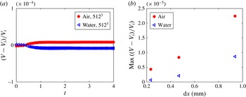
). As shown in appendix A, errors in mass (or volume) conservation are very small in the present numerical method (Popinet Reference Popinet2003, Reference Popinet2009). We have checked here that mass is conserved to better than 0.01 % for both air and water for all resolutions tested and better than 0.001 % in the highest resolution case (equivalent to
 $1024^{3}$
, see appendix A).
2.3 Initial conditions and physical parameters
We study a single breaking wave as was done in a previous 2-D study (Deike et al. Reference Deike, Popinet and Melville2015), but now extending it to three dimensions.
A third-order Stokes wave solution for the interface
 ${\it\eta}(x,y)$
and the velocity potential
 ${\it\phi}(x,y,z)$
in the water are used as initial conditions in a square box of size
 ${\it\lambda}$
on a side (see Deike et al. (Reference Deike, Popinet and Melville2015)). The wave propagates in the
 $x$
direction. Boundary conditions are periodic in
 $x$
and
 $y$
, and the top and bottom walls are free slip (at
 $z=\pm H={\it\lambda}/2$
). The wave slope
 $S=ak$
, with
 $a$
the initial wave amplitude and
 $k=2{\rm\pi}/{\it\lambda}$
the wavenumber, varies from 0.35 to 0.65, i.e. from incipient wave breaking to strongly plunging waves (Deike et al.
Reference Deike, Popinet and Melville2015). Note that since we are using only the third-order Stokes wave solution, slopes higher than the limiting slope for the full Stokes wave solution can be defined.
The density and viscosity ratios of the two phases are those of air and water. The Bond number
 $Bo={\rm\Delta}{\it\rho}g/({\it\gamma}k^{2})$
, with
 ${\rm\Delta}{\it\rho}$
the density difference between the two fluids,
 $g$
the gravity and
 ${\it\gamma}$
the surface tension, gives the ratio between gravity and surface tension forces. Due to computer limitations, related to the range of scales we are able to resolve, we choose
 $Bo=200$
. That corresponds to
 ${\it\lambda}=24$
cm in air–water conditions; large enough to generate a plunging breaker while also including the surface tension effect necessary to correctly resolve bubbles and droplets. The Reynolds number in the liquid is defined by
 $Re=c{\it\lambda}/{\it\nu}$
, with
 $c=\sqrt{g/k}$
the linear deep-water gravity-wave phase speed and
 ${\it\nu}$
the kinematic viscosity of the liquid (water). Again, due to computer limitations, related to spatial resolution constraints, we use
 $Re=40\,000$
, to correctly resolve the viscous boundary layer and still be at a large Reynolds number. This value is smaller than the one for a real
 $24$
cm wave by approximately a factor of 3, but should not affect qualitatively the results since we are at a sufficiently high Reynolds number (Deike et al.
Reference Deike, Popinet and Melville2015).
Adaptive mesh refinement is used to accurately solve for the interface and the vortical structures, with an equivalent grid resolution of
 $512^{3}$
for most of the runs, leading to a mesh size
 ${\it\lambda}/512\approx 0.4$
mm on the interface. This configuration allows accurate solutions for the dissipative scales, as shown by previous two-dimensional simulations (Deike et al.
Reference Deike, Popinet and Melville2015) and all the relevant length scales of the bubble formation problem: the wave scale, the capillary length (
 $l_{gc}=\sqrt{{\it\gamma}/({\rm\Delta}{\it\rho}g)}$
) and the Hinze scale.
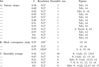
Parameters of the three sets of DNS of three-dimensional breaking waves,
 $Bo=200$
,
 $Re=40\,000$
. The last column indicates in which figures of the paper the data are used.

The energy components of the propagating wave can easily be obtained by integration over the whole volume,
 $\mathscr{V}$
, of air and water and are respectively the kinetic energy,
 $E_{k}=1/2\int _{\mathscr{V}}{\it\rho}\boldsymbol{u}^{2}\,\text{d}\mathscr{V}$
, the gravitational potential energy,
 $E_{g}=\int _{\mathscr{V}}{\it\rho}gz\,\text{d}\mathscr{V}+{\it\lambda}/8$
, where the constant
 ${\it\lambda}/8$
comes from the fact that the bottom of the box,
 $z=-{\it\lambda}/2$
, is used as a vertical datum (Chen et al.
Reference Chen, Kharif, Zaleski and Li1999) and the surface tension potential energy,
 $E_{s}={\it\gamma}(\mathscr{L}-{\it\lambda}^{2})$
, where
 $\mathscr{L}$
is the surface area of the interfaces including those of the bubbles. The total energy is then
 $E=E_{k}+E_{g}+E_{s}$
. In the following, these quantities will be given per unit length of breaking crest, i.e. divided by the width of the simulation box
 ${\it\lambda}$
. Note also that the length of the breaking crest
 $L_{c}$
is the width of the simulation box,
 $L_{c}={\it\lambda}$
.
2.4 Summary of the runs
Three sets of numerical experiments are presented and summarized in table 1. The A set of experiments consists of 12 runs for waves with various initial slopes (from
 $S=0.35$
to
 $S=0.65$
), with no initial perturbation in the transverse
 $y$
direction. The B set of experiments is a mesh size dependence study and is described in appendix A. Three runs are performed with increasing resolutions (and same initial slope,
 $S=0.55$
, corresponding to a plunging breaker) and show that the results are not changed for resolution finer than a grid equivalent to
 $512^{3}$
. Finally, the third set of experiments consists of ensemble averages for 5 different initial slopes
 $S$
in the same range as before. For each slope
 $S$
, between 6 and 10 runs are performed with some initial perturbation in the transverse direction
 $y$
. An example of the obtained data set and the ensemble-averaged results is given in appendix B. It shows good statistical convergence and that small perturbations do not significantly change the wave dissipation and bubble dynamics; however, the ensemble averaging improves the statistical convergence of the bubble size distribution. Table 1 also shows in which figure the various runs are used.
3 Wave breaking dynamics, air entrainment and energy dissipation
3.1 Wave breaking
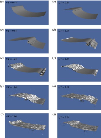
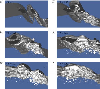
Figure 3 shows the interface
 ${\it\eta}(x,y,t)$
evolution with time for a plunging breaker of initial slope
 $S=0.55$
. The dynamics of a plunging breaker has been described by several authors. A jet forms in front of the wave (a,b), strikes the surface (c) and falls back to the surface due to gravity. Before the jet reconnects, the wave dynamics remains mostly two-dimensional. Air entrainment then occurs through different mechanisms, recently summarized in the review by Kiger & Duncan (Reference Kiger and Duncan2012): the entrapment of an air pocket when the jet reconnects the water, entraining a large cavity and large bubbles; entrainment around the jet impact site entraining smaller bubbles; entrapment by the subsequent splashes events; entrainment by the turbulent breakdown of the forward face of the wave. Indeed, numerous bubbles and droplets are visible (c–e) while the flow has become fully three-dimensional. Entrainment of air also occurs when the jet impacts the surface (c), during the subsequent splashing (d,e), and when high velocity droplets fall back into the water (f,g). As discussed by Deane & Stokes (Reference Deane and Stokes2002), Kiger & Duncan (Reference Kiger and Duncan2012), there are two main steps in bubble formation, first, when the jet impacts the water surface, creating relatively small bubbles and second when the air cavity collapses, creating larger bubbles that are then fragmented by turbulent fluctuations. Up to a thousand bubbles are counted in this simulation (f,g). The bubble cloud is very dense just after impact (f–h), and then bubbles rise to the surface and burst, with the larger bubbles rising faster (i–l). The waves then continue to propagate leaving the bubble cloud behind.
Snapshots of 3-D Gerris DNS solutions for the interface at different times for a plunging breaker,
 $S=0.55$
and a
 $1024^{3}$
equivalent resolution. (a,b) Formation of the jet; (c) impact and entrainment of the initial air pocket; (d,e) splashing and fragmentation of the air pocket; (f,g) splashing and bursting of large bubbles; (h–j) large dense bubble plume with numerous bubbles of various sizes in the water, together with droplets in the air.

Figure 4 shows a view from the bottom of the same simulation, revealing insights on the entrainment and bubble break-up process. After the wave impact, we can see the large air cavity entrained in the water, together with some satellite bubbles of small size (a). Just after the initial entrainment of the cavity, it is connected to the main ambient gas phase by thin filaments of air (b). These filaments of air are commonly observed under breaking waves in surf movies and were recently discussed in detail by Lubin & Glockner (Reference Lubin and Glockner2015). Later on, the cavity starts to collapse, creating both large and small bubbles (c,d). Once the cavity is completely destroyed, we observe a dense bubble plume, with bubble radii varying over more than one order of magnitude.
Bottom view of the simulation, showing the entrainment and collapse of the air cavity during the breaking event. (a) Just after impact, the tube of air is already formed inside the water, with some small satellite bubbles nearby. (b) The air cavity has started to collapse and is connected to the main surface by thin filaments of air. Bubbles of various sizes start to be visible. In (c,d) the cavity continues to collapse, with numerous bubbles of various sizes. In (e,f) the cavity has completely collapsed and a dense bubble plume is visible, with bubbles with radii varying over one order of magnitude.

The evolution of the wave is similar for the various plunging breakers
 $S\gtrsim 0.42$
, with increasing slopes leading to an increase of the entrained air. For smaller slopes, a spilling process is observed (
 $0.35\lesssim S\lesssim 0.42$
), with dynamics similar to that described experimentally by Rojas & Loewen (Reference Rojas and Loewen2010).
3.2 Energy dissipation
The first step is to verify that we correctly capture the wave dissipation properties in the present 3-D work. Wave energy dissipation due to breaking can be written as
 $E_{diss}=\int {\it\epsilon}_{l}{\it\Lambda}(\boldsymbol{c})\,\text{d}\boldsymbol{c}$
, with
 ${\it\epsilon}_{l}$
the dissipation per unit length of breaking crest and
 ${\it\Lambda}(\boldsymbol{c})\,\text{d}\boldsymbol{c}$
the mean length of breaking wave fronts moving at phase velocities in the range
 $(\boldsymbol{c},\boldsymbol{c}+d\boldsymbol{c})$
(Phillips Reference Phillips1985). The breaking distribution
 ${\it\Lambda}(\boldsymbol{c})$
can be measured in the field (Melville & Matusov Reference Melville and Matusov2002; Gemmrich, Banner & Garrett Reference Gemmrich, Banner and Garrett2008; Thomson, Gemmrich & Jessup Reference Thomson, Gemmrich and Jessup2009; Kleiss & Melville Reference Kleiss and Melville2010; Sutherland & Melville Reference Sutherland and Melville2013), while the dissipation
 ${\it\epsilon}_{l}$
is related to the fluid properties and the breaking kinematics (Duncan Reference Duncan1981; Phillips Reference Phillips1985),
 $$\begin{eqnarray}{\it\epsilon}_{l}=b{\it\rho}c^{5}/g,\end{eqnarray}$$
where
 $g$
is gravity,
 ${\it\rho}$
the water density,
 $c$
the characteristic phase speed of the breaking front and
 $b$
the non-dimensional breaking parameter.
The local time-averaged dissipation rate
 $\bar{{\it\varepsilon}}$
is related to the dissipation rate per unit breaking crest length,
 ${\it\epsilon}_{l}$
, by (Drazen, Melville & Lenain Reference Drazen, Melville and Lenain2008)
 $$\begin{eqnarray}{\it\epsilon}_{l}={\it\rho}A\bar{{\it\varepsilon}},\end{eqnarray}$$
with
 $A={\rm\pi}h^{2}/4$
representing the cross-sectional area of the entrained cylinder of air. This assumes that the turbulence is homogenous in the cylinder of cross-sectional area
 $A$
created by the breaking event (Drazen et al.
Reference Drazen, Melville and Lenain2008). The relationship between
 $\bar{{\it\varepsilon}}$
and the wave height at breaking
 $h$
is given by the inertial scaling for breaking waves (Drazen et al.
Reference Drazen, Melville and Lenain2008):
 $\bar{{\it\varepsilon}}={\it\Xi}h^{1/2}(2g)^{3/2}$
, with
 ${\it\Xi}$
an
 $O(1)$
constant. This leads to
 ${\it\epsilon}_{l}={\it\Xi}{\it\rho}g^{3/2}h^{5/2}{\rm\pi}/\sqrt{2}$
which combined with (3.1) gives
 $$\begin{eqnarray}b={\it\Xi}\frac{{\rm\pi}}{\sqrt{2}}(hk)^{5/2},\end{eqnarray}$$
where
 $hk$
is a measure of the wave slope at breaking. Drazen et al. (Reference Drazen, Melville and Lenain2008) have shown that the slope at breaking,
 $hk$
, is approximatively proportional to the linearly predicted maximum slope,
 $S$
, of a focusing packet. Romero, Melville & Kleiss (Reference Romero, Melville and Kleiss2012) derived the following semi-empirical relation for the breaking parameter initially based on laboratory data,
 $$\begin{eqnarray}b=0.4(S-0.08)^{5/2},\end{eqnarray}$$
where
 $S_{0}=0.08$
is a measure of the threshold for breaking and 0.4 an evaluation of the constant
 ${\it\Xi}{\rm\pi}/2$
. This inertial model, based on a simple physical argument for strong plunging waves, has been confirmed through extensive experimental studies and modelling well beyond the region of validity of the initial hypothesis (Romero et al.
Reference Romero, Melville and Kleiss2012; Grare et al.
Reference Grare, Peirson, Branger, Walker, Giovanangeli and Makin2013; Pizzo & Melville Reference Pizzo and Melville2013; Melville & Fedorov Reference Melville and Fedorov2015; Deike et al.
Reference Deike, Popinet and Melville2015). Note that proportionality between the initial slope and the slope at breaking is also true in our DNS of steep Stokes waves, and following the definition of Drazen et al. (Reference Drazen, Melville and Lenain2008) where
 $h$
is the vertical distance the breaking wave toe travels before impact,
 $hk=-0.05+S$
for both the 3-D DNS presented here and the 2-D results presented in Deike et al. (Reference Deike, Popinet and Melville2015). In the following we now consider
 $S$
as our initial wave slope.
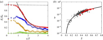
(a) Wave energy as a function of time: (▫) total energy; (○) kinetic energy; (▿) gravitational potential energy; (♢) surface tension potential energy. The solid line is an exponential fit
 $E=E_{0}e^{-{\it\zeta}t}$
for
 $1<t/T<2$
, and the dashed line is the linear viscous decay
 $E=E_{0}e^{-2{\it\nu}k^{2}t}$
. (b) Breaking parameter
 $b$
as a function of the initial wave slope
 $S$
. (▾) DNS data. Solid line: semi-empirical formulation based on a scaling argument, (3.4),
 $b=0.4(S-0.08)^{5/2}$
from Romero et al. (Reference Romero, Melville and Kleiss2012). Black and grey symbols are experimental data; black and grey triangles and grey diamonds are from Drazen et al. (Reference Drazen, Melville and Lenain2008), crosses and circles are from Banner & Peirson (Reference Banner and Peirson2007) and squares are from Grare et al. (Reference Grare, Peirson, Branger, Walker, Giovanangeli and Makin2013). The differences between experiments and DNS at lower values of
 $S$
come from differences in initiating wave breaking.

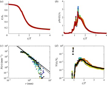
Figure 5(a) shows the evolution with time of the total wave energy
 $E$
per unit length of breaking crest, together with the kinetic and potential components. An abrupt decrease of the total wave energy is observed when the wave breaks, with most of the wave energy lost during the first wave period. The energy decay can be fitted by an exponential during this time period,
 $E=E_{0}\exp (-{\it\zeta}t)$
, with
 ${\it\zeta}$
the observed decay rate and
 $E_{0}$
the initial wave energy per unit length of crest. The dissipation rate per unit breaking crest is then simply given by
 ${\it\epsilon}_{l}=E_{0}{\it\zeta}$
(or by taking
 ${\it\epsilon}_{l}=-{\rm\Delta}E/{\it\tau}_{b}$
, where
 ${\it\tau}_{b}$
is the active breaking time and
 ${\rm\Delta}E$
the energy difference before and after breaking, both estimations being equivalent). The breaking parameter is then
 $b={\it\epsilon}_{l}g/({\it\rho}c^{5})$
, with
 $c$
the linear phase speed of the wave.
Figure 5(b) shows
 $b$
as a function of the initial wave slope
 $S$
in the DNS, and we observe a very good agreement for strong plunging waves with the semi-empirical result given by (3.4) initially derived from laboratory data (Drazen et al.
Reference Drazen, Melville and Lenain2008; Romero et al.
Reference Romero, Melville and Kleiss2012), see also data from Grare et al. (Reference Grare, Peirson, Branger, Walker, Giovanangeli and Makin2013) and 2-D numerical simulations from Deike et al. (Reference Deike, Popinet and Melville2015). This confirms that the present 3-D DNS captures the dissipative scales of the breaking wave process. The total dissipation due to breaking in the 3-D DNS is very similar to the one obtained in 2-D DNS reported by Deike et al. (Reference Deike, Popinet and Melville2015). The difference in the dissipation between experiments and DNS for
 $S$
between 0.35 and 0.4 is most likely related to the route to breaking, i.e. how the initial data are set up. Indeed, as discussed in Deike et al. (Reference Deike, Popinet and Melville2015), the critical slope for wave breaking changes when a steep Stokes wave is used instead of wave focusing packet or modulational instability in the laboratory. In the present case, a slope of
 $0.35$
corresponds to an incipient breaking wave, which has total dissipation less than a spilling breaker of the same slope obtained by a wave focusing technique in the laboratory.
3.3 Air entrainment and void fraction
Experimentally, the local void fraction
 ${\it\alpha}(x,z,t)$
(volume of air per unit volume of air–water mixture) is measured using conductivity (Lamarre & Melville Reference Lamarre and Melville1991) or optical probes (Blenkinsopp & Chaplin Reference Blenkinsopp and Chaplin2007; Rojas & Loewen Reference Rojas and Loewen2007). A spatial map of the void fraction is then obtained by repeating this measure at various locations. In order to compare our simulations with the experimental description of the two-phase air–water flow during the breaking event, we compute an equivalent of this experimentally measured void fraction, by averaging the tracer
 $\mathscr{T}$
over the transverse direction
 $y$
:
 $$\begin{eqnarray}{\it\alpha}(x,z,t)=\frac{1}{L_{c}}\int _{-L_{c}/2}^{L_{c}/2}\mathscr{T}(x,y,z,t)\,\text{d}y,\end{eqnarray}$$
where
 $L_{c}={\it\lambda}$
is the size of the domain in the transverse
 $y$
direction (and corresponds to the length of breaking crest). This measure of the void fraction can then be integrated in space in order to obtain another estimate the amount of air entrained by the breaking wave. The main interface during the breaking process can then be defined by the
 ${\it\alpha}(x,z,t)=50\,\%$
value, as proposed experimentally by several authors (Lamarre & Melville Reference Lamarre and Melville1991; Blenkinsopp & Chaplin Reference Blenkinsopp and Chaplin2007).
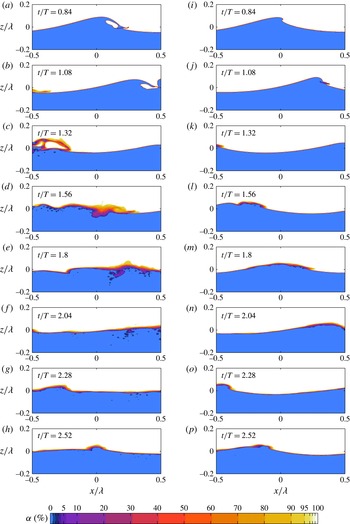
Transversally integrated void fraction
 ${\it\alpha}(x,z,t)=1/L_{c}\int _{-L_{c}/2}^{L_{c}/2}\mathscr{T}(x,y,z,t)\,\text{d}y$
, (in %), from the 3-D data, at different times. (a–h) Plunging breaker (
 $S=0.55$
). (i–p) Spilling breaker (
 $S=0.42$
). Colour scale is nonlinear in order to reveal variations towards the extremes of the range.

Figure 6 shows the evolution of the void fraction (volume of air per unit volume of air–water mixture),
 ${\it\alpha}(x,z,t)$
, during the breaking process, for a plunging breaker (
 $S=0.55$
) and a spilling breaker (
 $S=0.42$
).
In the plunging case, the impact of the jet reveals again the various air entrainment processes, the entrapment of a large air pocket (a,b), as well as the rebound (b,c) and entrainment by the turbulent breakdown of the forward face. Spray generation is observed during the splashing process (c,d). Bubble plumes are formed during these entrainment processes and high void fraction areas are visible (c–f). The bubble plume appears very dense and consists predominantly of large air cavities that collapse into smaller bubbles and are driven down into the water, reaching a maximum penetration depth (d–f). Then the bubble clouds spread horizontally and large bubbles and air cavities rise back to the surface to burst, corresponding to the fast degassing stage (e–g). These events correspond to the active breaking stage. Smaller void fraction features remain for longer times (g,h), corresponding to the small bubbles with low rise velocities. Eventually, even the smaller bubbles rise back to the surface. This stage corresponds to the decay of the breaking event. The bubble cloud dynamics as well as the void fraction observed during the breaking are consistent with previous experimental observations (Lamarre & Melville Reference Lamarre and Melville1991, Reference Lamarre and Melville1994; Blenkinsopp & Chaplin Reference Blenkinsopp and Chaplin2007): the air cavity is first entrained with
 ${\it\alpha}=100\,\%$
, collapses and gives birth to a bubble cloud with
 ${\it\alpha}$
up to
 $30\,\%$
during the active breaking stages.
In the spilling case, the breaking process is started by the appearance of a rough surface or of a small jet at the wave crest (i), then a small region of turbulence forms at the crest of the wave, and this region grows as water spills down the face of the wave (j,k). As the wave spills, air is entrained and spray is ejected at the leading edge of the breaker (k,l) and relatively shallow bubble clouds are formed beneath the surface (l–o). This general scenario is in agreement with experimental observations from Rojas & Loewen (Reference Rojas and Loewen2010). As for the plunging case, larger bubbles rise back to the surface and burst while smaller ones remain longer in the water column (m–p).
3.4 Time evolution of the bubble size distribution and integral quantities
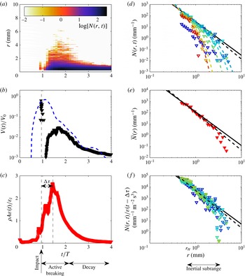
Ensemble-averaged data for a plunging breaker (
 $S=0.55$
) (a) time evolution of the bubble size distribution
 $N(r,t)$
. Colour is in log-scale. (b) Time evolution of the volume of entrained air
 $V(t)/V_{0}$
, with
 $V_{0}=AL_{c}$
, calculated from the closed surfaces (▾) and from the void fraction (blue line). (c) Time evolution of the energy dissipation
 ${\it\rho}A{\it\varepsilon}(t)/{\it\epsilon}_{l}$
(red symbols). A delay between the time
 ${\it\varepsilon}(t)$
and
 $V(t)$
maxima is clearly visible. (d) Bubble size distribution
 $N(r,t)$
at different times
 $t$
. Time is colour coded. Dashed lines are
 $N(r,t)\propto r^{-m}\text{e}^{[-K(r/r_{m}(t))^{2}]}$
, with
 $K=2$
and
 $r_{m}(t)$
decreasing with time. (e) Active breaking time-averaged bubble size distribution
 $\bar{N}(r)$
: the dashed line is
 $\bar{N}(r)\propto r^{-10/3}$
and the solid line is
 $\bar{N}(r)\propto r^{-3}$
. (f) Rescaled bubble size distribution
 $N(r,t)/{\it\varepsilon}(t-{\rm\Delta}{\it\tau})$
during the active breaking stage, from
 $t/T=1.2$
to
 $t/T=2.4$
.
 ${\rm\Delta}{\it\tau}$
is the delay time between the maximum entrained air and the maximum dissipation, corresponding to the turbulent break-up time. Time is colour coded as in (d).

Here we describe the time evolution of the bubble plume properties (volume and size distribution) for the strong plunging wave,
 $S=0.55$
shown in figures 3, 4, 5(a) and 6. The data are obtained from ensemble averaging 6 runs with small initial perturbations in the transverse wave direction
 $y$
. As shown in appendix B, the ensemble averaging improves the bubble statistics.
Figure 7(a) shows the time evolution of the bubble size distribution
 $N(r,t)$
. When the jet reconnects to the water surface (
 $t/T\approx 1$
), a large pocket of air is entrained in the water. This pocket of air collapses and bubbles of various sizes are formed. Bubbles between 2 mm and the mesh size are first created at the impact (
 $t/T\approx 1$
), then a rapid growth of the bubble size distribution is observed (
 $1\lesssim t/T\lesssim 1.6$
), with bubbles as large as 10 mm, corresponding to the collapse of the air cavity. Therefore, bubbles of various sizes are created during the initial impact and entrapment of the air cavity (visible in figure 4), due to entrainment by the jet, and at the edges of the air cavity, as discussed by Deane & Stokes (Reference Deane and Stokes2002) and Kiger & Duncan (Reference Kiger and Duncan2012). The maximum number of bubbles in the system is reached at the end of this growing stage. A fast decay is then observed (
 $1.6\lesssim t/T\lesssim 2.4$
). Large bubbles are the first to disappear, collapsing or rising back to the surface and bursting. These two stages define the active breaking time. Finally, a slower decay of the size distribution is observed (
 $t/T>2.4$
, decay stage) where small bubbles slowly rise to the surface.
Figure 7(b) shows the evolution with time of the entrained volume of air
 $V(t)/V_{0}$
, where
 $V_{0}=AL_{c}={\rm\pi}h^{2}L_{c}/4$
is the reference maximum volume of air that can be entrained during the active breaking process. The volume of air is defined by the sum over all closed surfaces (bubbles of volume
 $v_{i}^{a}$
),
 $V=\sum _{i\geqslant 1}v_{i}^{a}$
, as described in § 2. The first peak observed at
 $t/T\approx 1$
corresponds to the impact of the jet and the entrapment of a large pocket of air, with a cross-sectional area that is almost (
 $V=0.9V_{0}$
) the reference tube of air of surface
 $A$
, visible in figures 2, 4 and 5. The measured volume of air then decreases because of the collapse of the initial tube and its topological reconnection to the water surface during this highly turbulent event (as shown in figure 4(b)).
Then, bubbles are formed and a second maximum of the volume of air, which corresponds to the moment where the largest number of bubbles is present in the system. This second maximum is one order of magnitude smaller than the volume of the initial tube. The fraction of air that remains trapped in the water corresponds to the rapid and continuous increase of
 $V(t)$
for
 $1\lesssim t/T\lesssim 1.6$
. Then
 $V(t)$
decreases, quickly over approximately one wave period
 $1.6\lesssim t/T\lesssim 2.4$
. As described by Lamarre & Melville (Reference Lamarre and Melville1991), the fast decay is exponential, with
 $V=V_{0}\exp (-{\it\kappa}t/T)$
, with
 ${\it\kappa}$
a numerical factor varying from approximately 2.5 to 4 in our DNS, depending on the initial wave slope. These values appear in reasonable agreement with the experimental values, considering the difficulty of the experiments of Lamarre & Melville (Reference Lamarre and Melville1991) and Blenkinsopp & Chaplin (Reference Blenkinsopp and Chaplin2007), who found
 ${\it\kappa}=3.9$
and
 ${\it\kappa}\approx 5$
, respectively. This rapid decay corresponds to the fast degassing of the plume caused by large bubbles rising back to the surface. The growing stage and the fast decay correspond to the active breaking stages, lasting slightly longer than one wave period. It is followed by a slower decay, that was also observed experimentally by Lamarre & Melville (Reference Lamarre and Melville1994).
Note that the abrupt decrease of air is related to the fact that the tube of air collapses and is partially reconnected to the air above the wave (as in figure 4(b)). If we follow the definitions used in laboratory experiments and compute the volume of entrained air based on the void fraction (Lamarre & Melville Reference Lamarre and Melville1991; Blenkinsopp & Chaplin Reference Blenkinsopp and Chaplin2007):
 $$\begin{eqnarray}V_{{\it\alpha}}(t)=L_{c}\int _{-L}^{L}\,\text{d}x\int _{-H}^{{\it\alpha}=50\,\%}{\it\alpha}(x,z,t)\,\text{d}z,\end{eqnarray}$$
with
 ${\it\alpha}(x,z,t)=50\,\%$
considered as the main wavy interface (and
 $L={\it\lambda}$
the size of the numerical domain in the
 $x$
direction), then we observe a monotonic decay after the initial entrainment of the air cylinder at
 $t/T=1$
(as in the experiments). The two measures of the volume give the same result for the maximum volume of entrained air and for the time evolution after
 $t/T=1.6$
.
Figure 7(c) shows the spatially averaged turbulent dissipation rate
 ${\it\varepsilon}(t)$
(normalized by
 ${\it\epsilon}_{l}/({\it\rho}A)$
) as a function of time
 $t$
(normalized by the wave period
 $T$
). Its evolution follows closely the volume of entrained air
 $V(t)$
, with a clear time delay
 ${\rm\Delta}{\it\tau}$
between the maxima of
 ${\it\varepsilon}(t)$
and
 $V(t)$
. The dissipation rate first increases during the air entrainment and splashing processes and then decreases during the degassing process. Note that during the active breaking stages, the instantaneous turbulent dissipation rate
 ${\it\rho}A{\it\varepsilon}(t)$
is of the same order of magnitude as the dissipation rate per unit length of breaking crest
 ${\it\epsilon}_{l}$
obtained from the decay of the wave energy (see figure 5). When averaging in time, we obtain indeed
 ${\it\rho}A\bar{{\it\varepsilon}}={\it\epsilon}_{l}$
. The time lag between the maximum in the volume of entrained air and the peak in the dissipation can be assigned to the fragmentation time of the initial air pocket.
Figure 7(d) shows
 $N(r,t)$
at given times
 $t$
during the active breaking period and the decay stage. The time is colour coded. During this active breaking time (
 $1.2\leqslant t/T\leqslant 2.4$
), the dependence on the radius is adiabatic in time, i.e the size distribution follows
 $N(r,t)\propto r^{-m}$
, with
 $3\leqslant m\leqslant 3.5$
constant with time, within the error bars.
The amplitude of the bubble size distribution first grows (from dark blue to light blue), reaches a maximum (
 $t/T\approx 1.9$
, light blue) and then decays (from light green to red), following, with a time delay, the time evolution of both
 ${\it\varepsilon}(t)$
and
 $V(t)$
. During this stage, the bubble cascade inertial subrange, i.e. the range of scales for which the power law is observed, starts close to the smallest scale resolved in the simulation and ends at approximately 4 mm. The time evolution of
 $N(r,t)$
is in agreement with the experimental results from Blenkinsopp & Chaplin (Reference Blenkinsopp and Chaplin2010), where the bubble size distribution is found to follow a power law with
 $m\approx 3$
roughly constant during the active breaking stage.
After the active breaking stage (
 $t/T>2.4$
, from yellow to red), the bubble size distribution rapidly decays, starting with the large bubbles, and a much steeper bubble size distribution is observed, in agreement with experimental results (Terrill et al.
Reference Terrill, Melville and Stramski2001; Deane & Stokes Reference Deane and Stokes2002). While Deane & Stokes (Reference Deane and Stokes2002) describe a steep power law (finding
 $m_{decay}=6$
), the bubble size distribution can also be described by an empirical decay function; combining the turbulent break-up law
 $N(r,t)\propto r^{-m}$
and an exponential decay, due to the scale-dependent rise of the bubbles that governs the decay of
 $N(r,t)$
. We propose the following empirical function:
 $$\begin{eqnarray}N(r,t)=N_{0}r^{-m}\exp \left[-K\left(\frac{r}{r_{m}(t)}\right)^{2}\right].\end{eqnarray}$$
Here
 $r_{m}(t)$
is the time-dependent variable,
 $K=2$
a constant empirical parameter and
 $m=10/3$
. Here
 $r_{m}(t)$
corresponds physically to a cutoff radius that decreases with time, and quantifies the fact that, due to the rise of the bubbles, the inertial subrange of the bubble cascade is reduced once the active breaking stage is over. The exponent
 $2$
inside the exponential functional form has been chosen to match the one giving the rise velocity of the bubbles (see below). For the times displayed in figure 7(e),
 $r_{m}(t)$
decreases linearly from 4 mm (
 $t/T=2.5$
, light blue) to 1 mm (
 $t/T=3.5$
, red). Thus the cutoff radius decreases until it reaches a value close to the Hinze scale. At this time, the turbulent motion is too weak and no more bubble cascade process is observed. Note that the semi-empirical formulation (3.7) can be applied to the experimental data of Deane & Stokes (Reference Deane and Stokes2002) shown in the inset of figure 1.
Figure 7(e) shows the time-averaged bubble size distribution
 $\bar{N}(r)$
over the active breaking time
 ${\it\tau}_{b}$
.
 $\bar{N}(r)$
is found to follow a power law,
 $\bar{N}(r)\propto r^{-m}$
, with
 $3\leqslant m\leqslant 3.5$
compatible with various experimental results (Terrill et al.
Reference Terrill, Melville and Stramski2001; Deane & Stokes Reference Deane and Stokes2002; Rojas & Loewen Reference Rojas and Loewen2007; Blenkinsopp & Chaplin Reference Blenkinsopp and Chaplin2010). The bubble inertial subrange, i.e. the range of bubble radii for which the power law is observed, starts close to the smallest resolved scale (approximately
 $0.8$
mm) and ends at the radius of the largest bubbles observed in the simulations (between
 $4$
and
 $6$
mm). The scale of the beginning of the bubble cascade corresponds to the Hinze scale (
 $r_{H}\approx 0.8$
mm using (1.2)). However, the mesh resolution is also close to this scale (
 $0.4$
mm) so the Hinze scale might not be fully resolved.
Note that, experimentally, various shapes for
 $r<r_{H}$
have been observed by Deane & Stokes (Reference Deane and Stokes2002), Leifer & de Leeuw (Reference Leifer and de Leeuw2006) and Blenkinsopp & Chaplin (Reference Blenkinsopp and Chaplin2010). We should also remark that it is clear from figure 7(d) that the exact value of the exponent
 $m$
depends on the time chosen to average the bubble size distribution. Indeed, if one averaged over the active breaking and decay stage, one would obtain a steeper size distribution and a higher value for
 $m$
. We believe that this sensitivity in the time of observation is at least partially responsible for the relatively wide range of values observed for
 $m$
in the literature, due to the difficulty in properly identifying the active breaking time.
Finally, we discuss the scaling of
 $N(r,t)$
with
 ${\it\varepsilon}(t)$
during the active breaking stages. Figure 7
f shows the size distribution is indeed well described by
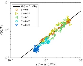
 $N(r,t)\propto {\it\varepsilon}(t-{\rm\Delta}{\it\tau})r^{-m}$
, with
 $3\leqslant m\leqslant 3.5$
independent of time and
 ${\rm\Delta}{\it\tau}$
the time lag related to the fragmentation of the initial air pocket. The time is colour coded as in figure 7(d). This description is valid, within the scatter of the data, for the active breaking stages that last more than one wave period (
 $1.2\leqslant t/T\leqslant 2.4$
).
The time evolution of the entrained air phase can be used to define the active breaking stage; similarly to what was done experimentally using measurement of the noise generated by the bubbles (Drazen et al.
Reference Drazen, Melville and Lenain2008). The active breaking stage starts when the jet impacts the water surface and ends when the adiabatic bubble size distribution is no longer observed, so that its total duration here is
 ${\it\tau}_{b}\approx 1.2T$
.
The overall patterns of evolution of the volume of air, the dissipation rate and the bubble size distribution are similar for all plunging and spilling breakers we have investigated.
3.5 Decay time and rise velocities
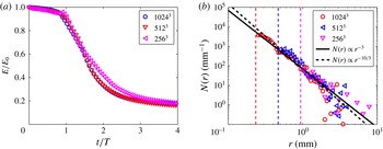
The time evolution of the number of bubbles at a given scale,
 $r$
, is shown in figure 8 normalized by its maximum
 $N(r,t)/N_{0}(r)$
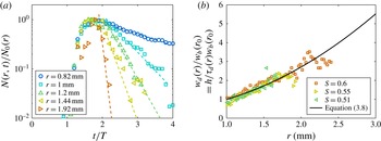
. Large bubbles are created first but the time delay between the maximum number of bubbles for various radii is small, indicating fast bubble break-up processes. Large bubbles are seen to disappear first and much faster than the smaller bubbles. The decay rate
 ${\it\tau}_{d}(r)$
of bubbles of radius
 $r$
can be measured by fitting the decay of the bubble size distribution by
 $N(r,t)=N_{0}(r)e^{-t/{\it\tau}_{d}(r)}$
. This decay rate includes both the rise of the bubbles, and the collapse of the large bubbles into smaller ones. However, since we consider the decay starting at the end of the active breaking stage, the dominant process should be the rise of the bubble. From this decay rate, we can estimate an average bubble velocity by assuming that the path of the bubbles is given by the distance the bubble has to rise to reach the surface, which corresponds to the average penetration depth of the bubble cloud, say
 $h$
. Thus we define the scale-dependent decay velocity of the bubble size distribution by
 $w_{d}(r)=h/{\it\tau}_{d}(r)$
, with
 $w_{d}(r)$
shown in figure 8(b) for three plunging breakers.
(a) Time evolution of
 $N(r,t)$
for
 $S=0.55$
and various radii
 $r$
. Dashed lines are exponential fits,
 $N(r,t)/N_{0}(r)=e^{-t/{\it\tau}_{d}(r)}$
. (b) Decay velocity
 $w_{d}(r)=h/{\it\tau}_{d}(r)$
compared to the rise velocity of bubbles
 $w_{b}$
(solid line) given by (3.8). Velocities are rescaled by
 $w_{b}(r_{0}=1~\text{mm})$
.

The rise velocity of a bubble of radius
 $r$
in clean water (for radius larger than
 $100~{\rm\mu}\text{m}$
) is given by Woolf & Thorpe (Reference Woolf and Thorpe1991) (see also Thorpe (Reference Thorpe1982) for a review of bubble rise velocities),
 $$\begin{eqnarray}w_{b}=\frac{gr^{2}}{{\it\nu}_{w}}\frac{1}{18[1-2/(1+0.091{\it\chi})^{1/2}]},\quad \text{with }{\it\chi}=\frac{gr^{3}}{{\it\nu}_{w}^{2}}.\end{eqnarray}$$
Figure 8 shows that the decay velocity of the bubbles
 $w_{d}(r)=h/{\it\tau}_{d}(r)$
is close to the rise velocity of bubbles in clean water
 $w_{b}$
(3.8). Thus the decay of the bubble plume (for
 $t/T>2$
) is consistent with the bubbles rising back to the surface.
3.6 Time-averaged bubble size distribution
We now discuss the time-averaged (over the active breaking time
 ${\it\tau}_{b}$
) bubble size distribution
 $\bar{N}(r)$
for various wave slopes,
 $S$
, and the relationship with the wave dissipation rate per unit length of breaking crest,
 ${\it\epsilon}_{l}$
.
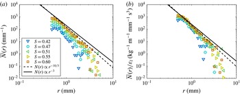
Ensemble-averaged data for 5 breaking waves with initial slopes from
 $S=0.42$
to
 $S=0.6$
. Time-averaged bubble size distribution
 $\bar{N}(r)$
over the active breaking time
 ${\it\tau}_{b}$
. (a)
 $\bar{N}(r)$
,
 $S$
(colour scaled) increasing from bottom to top. The number of bubbles increases with
 $S$
. (b) Rescaled bubble size distribution
 $\bar{N}(r)/{\it\epsilon}_{l}$
. The data collapse significantly between (a) and (b); except for the smaller slopes where the inertial break-up subrange is of limited extent. In both plots, the dashed line is
 $\bar{N}(r)\propto r^{-10/3}$
and the solid line is
 $\bar{N}(r)\propto r^{-3}$
.

Figure 9(a) shows the time-averaged bubble size distribution,
 $\bar{N}(r)$
, for increasing initial wave slope. The bubble size distribution follows a power law,
 $\bar{N}(r)\propto r^{-m}$
with
 $3\leqslant m\leqslant 3.5$
, from the Hinze scale to a cutoff radius,
 $r_{m}$
, that increases with
 $S$
. The amplitude of
 $\bar{N}(r)$
as well as the range of bubble radii for which the power law is observed increase with the wave slope,
 $S$
. Both are related to the increase of total volume of air entrained, the size of the initial air pocket trapped during the overturning and impact of the breaking wave and the increase of turbulence fluctuations with the slope,
 $S$
. For a large amplitude plunging breaker, the bubble break-up cascade subrange goes from approximately 0.8 to 5 mm while for smaller amplitude spilling breakers, the range of validity of the
 $\bar{N}(r)\propto r^{-m}$
relationship is smaller, the cutoff radius being approximately 3 mm, closer to the Hinze scale, due to a smaller amount of entrained air and weaker turbulent fluctuations.
Figure 9(b) shows the bubble size distribution rescaled by the dissipation rate per unit length of breaking crest
 ${\it\epsilon}_{l}$
,
 $\bar{N}(r)/{\it\epsilon}_{l}$
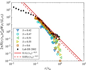
. A significant collapse of the data is observed within the bubble cascade subrange.
To summarize, we find that the dependence of the bubble size distribution on the bubble radius is the same for both the time-averaged data and the time-dependent data during the active breaking stage; both being proportional to
 $\propto r^{-m}$
,
 $3\leqslant m\leqslant 3.5$
for a wide range of initial slopes and for approximately one decade in radii. Moreover, the bubble size distribution scales with the turbulent dissipation rate, both when considering the time-dependent bubble size distribution
 $N(r,t)\propto {\it\varepsilon}$
and the time-averaged data
 $\bar{N}(r)\propto {\it\epsilon}_{l}$
, where
 ${\it\epsilon}_{l}={\it\rho}A\bar{{\it\varepsilon}}$
. While the constant-
 $Q$
model of Garrett et al. (Reference Garrett, Li and Farmer2000) describes the
 $r^{-m}$
scaling, it does not quantify
 $Q$
in terms of the other variables and is independent of time. In the next § 4, we discuss a new model that is consistent with the results of the DNS data.
4 A model for bubble size distribution
Here, we propose a new model to describe both the time-dependent bubble size distribution during the active breaking stage and the time-averaged results, combining ideas from the two models described in the Introduction and the results of the DNS.
4.1 Global balance between turbulent dissipation and work done against buoyancy forces
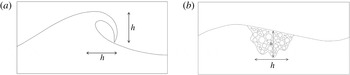
When a wave breaks, it entrains a tube of air of cross-sectional area
 $A\approx {\rm\pi}h^{2}/4$
, displayed in figure 10, creating a turbulent bubble cloud over a similar area for short times after the breaking onset. Here
 $h$
is the vertical distance between the crest of the breaker and its point of impact on the surface below and we assume geometrical similarity for the area
 $A$
across the range of wave slopes. We aim to describe the number of bubbles and their size distribution within this area. The bubble size distribution per unit volume
 $\mathscr{N}(r,t)$
is then related to the absolute bubble size distribution
 $N(r,t)$
by
 $$\begin{eqnarray}N(r,t)=V_{0}\mathscr{N}(r,t)=AL_{c}\mathscr{N}(r,t),\end{eqnarray}$$
with
 $V_{0}=AL_{c}={\rm\pi}h^{2}L_{c}/4$
the maximum volume of entrained air during breaking and
 $L_{c}$
the length of the breaking crest.
Sketch of the cross-sectional area of the air entrainment by a breaking wave: a tube of air of section
 $A\propto h^{2}$
is entrained (a) and creates a turbulent bubble cloud over a similar area (b).

The core of the model is to use the simple assumption based on empirical data (Lamarre & Melville Reference Lamarre and Melville1991; Blenkinsopp & Chaplin Reference Blenkinsopp and Chaplin2007; Lim et al. Reference Lim, Chang, Huang and Na2015) that globally (integrating over space and time of the event) the work done against buoyancy forces in entraining the bubbles is proportional to the mechanical energy dissipated. This statement can be represented by the following equation:
 $$\begin{eqnarray}\int \int \int {\it\rho}g\mathscr{N}(r,\boldsymbol{x},t)\frac{4{\rm\pi}}{3}r^{3}w(\boldsymbol{x},t)\,\text{d}r\,\text{d}\boldsymbol{x}\,\text{d}t=B\int \int {\it\rho}(1-{\it\alpha}(\boldsymbol{x},t)){\it\varepsilon}(\boldsymbol{x},t)\,\text{d}\boldsymbol{x}\,\text{d}t,\end{eqnarray}$$
where
 ${\it\varepsilon}(\boldsymbol{x},t)$
is the local dissipation rate in the water,
 $w(\boldsymbol{x},\boldsymbol{t})$
the local vertical velocity of the bubble cloud and
 ${\it\alpha}(\boldsymbol{x},t)$
the void fraction (volume of air per unit volume), all functions of space
 $\boldsymbol{x}$
and time
 $t$
, and
 $B$
is a dimensionless constant.
Recall that
 ${\it\varepsilon}(\boldsymbol{x},t)$
is the local viscous dissipation rate,
 ${\it\varepsilon}(\boldsymbol{x},t)=2{\it\nu}\unicode[STIX]{x1D60B}_{ij}\unicode[STIX]{x1D60B}_{ij}$
, with
 $\unicode[STIX]{x1D60B}_{ij}\equiv (\partial _{i}u_{j}+\partial _{j}u_{i})/2$
(Pope Reference Pope2000). Therefore the total mechanical energy dissipated in the water is the integral over the volume of water and time
 $\int \int {\it\rho}(1-{\it\alpha}(\boldsymbol{x},t)){\it\varepsilon}(\boldsymbol{x},t)\,\text{d}\boldsymbol{x}\,\text{d}t$
, where the inclusion of the void fraction in the equation ensures the integration in the water only.
We first assume, for simplicity, that
 ${\it\alpha}\ll 1$
, and that the density of water
 ${\it\rho}$
is constant, so that (4.2) becomes
 $$\begin{eqnarray}\int \int \int g\mathscr{N}(r,\boldsymbol{x},t)\frac{4{\rm\pi}}{3}r^{3}w(\boldsymbol{x},t)\,\text{d}r\,\text{d}\boldsymbol{x}\,\text{d}t=B\int \int {\it\varepsilon}(\boldsymbol{x},t)\,\text{d}\boldsymbol{x}\,\text{d}t.\end{eqnarray}$$
Now let us assume that locally, the bubble size distribution is proportional to the turbulent dissipation rate, i.e.
 $\mathscr{N}\propto {\it\varepsilon}$
, which is supported by the DNS data (figure 7). The time lag between air entrainment and dissipation observed in the DNS results can be incorporated at this stage by setting,
 $\mathscr{N}\propto {\it\varepsilon}(t-{\rm\Delta}{\it\tau})$
; cf. figure 7.
With
 $\mathscr{N}\propto {\it\varepsilon}(t-{\rm\Delta}{\it\tau})$
, we now assume separation of variables to give
 $$\begin{eqnarray}\mathscr{N}(r,\boldsymbol{x},t)=R(r,r_{m}){\it\varepsilon}(\boldsymbol{x},t-{\rm\Delta}{\it\tau}),\end{eqnarray}$$
where
 $r_{m}$
is the maximum bubble size, then (4.3) becomes
 $$\begin{eqnarray}\int ^{r_{m}}gR(r,r_{m})\frac{4{\rm\pi}}{3}r^{3}\,\text{d}r\int \int {\it\varepsilon}(\boldsymbol{x},t-{\rm\Delta}{\it\tau})w(\boldsymbol{x},t)\,\text{d}\boldsymbol{x}\,\text{d}t=B\int \int {\it\varepsilon}(\boldsymbol{x},t)\,\text{d}\boldsymbol{x}\,\text{d}t.\end{eqnarray}$$
Therefore,
 $$\begin{eqnarray}\int ^{r_{m}}gR(r,r_{m})\frac{4{\rm\pi}}{3}r^{3}\,\text{d}r=BW^{-1},\quad \text{with }W=\frac{\int \int w(\boldsymbol{x},t){\it\varepsilon}(\boldsymbol{x},t-{\rm\Delta}{\it\tau})\,\text{d}\boldsymbol{x}\,\text{d}t}{\int \int {\it\varepsilon}(\boldsymbol{x},t)\,\text{d}\boldsymbol{x}\,\text{d}t},\end{eqnarray}$$
where
 $W$
is the dissipation-weighted vertical mean velocity of the bubble plume over the active breaking period. For any breaking event,
 $W$
and
 $r_{m}$
are constants and play parametric roles in further development of the model.
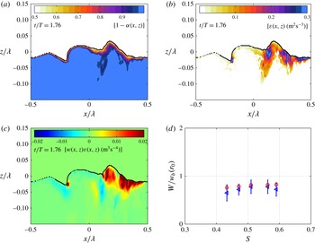
Here
 $W$
is the weighted vertical velocity of the bubble cloud and corresponds to an average rise velocity of the bubble plume, so that together with gravity, it can be interpreted as the variable corresponding to the bubble buoyancy forces. Taking into account
 $r_{m}$
in the dimensional analysis corresponds to considering the role of the maximum bubble size in the fragmentation process.
Now, equation (4.6) dimensionally constrains the scaling with respect to
 $W$
and
 $g$
, so that
 $$\begin{eqnarray}\mathscr{N}(r,\boldsymbol{x},t)\propto B\frac{{\it\varepsilon}(\boldsymbol{x},t-{\rm\Delta}{\it\tau})}{Wg}f(r,r_{m}),\end{eqnarray}$$
where
 $R(r,r_{m})\propto Bf(r,r_{m})/(Wg)$
. Seeking power-law solutions, with
 $f(r,r_{m})$
having the dimensions of
 $\mathscr{N}$
,
 $[L^{-4}]$
, we have
 $$\begin{eqnarray}\mathscr{N}(r,\boldsymbol{x},t)=B\frac{3(4-m)}{4{\rm\pi}}\frac{{\it\varepsilon}(\boldsymbol{x},t-{\rm\Delta}{\it\tau})}{Wg}r^{-m}r_{m}^{m-4},\end{eqnarray}$$
with
 $m<4$
to avoid divergence of (4.6). The
 $(4-m)$
constant is introduced to be consistent with the initial equation, (4.2) and cancels the numerical constant when integrating over all bubble radii. Note also that available experimental data and our numerical data suggest
 $3<m<4$
. At this point, we have a constraint on the prefactor of the bubble size distribution, i.e. on the total volume of air, but we need information on the statistics to determine
 $m$
.
Equation 4.8 can be justified by a dimensional analysis. Say
 $\mathscr{N}$
depends on the bubble scales, i.e. the radius
 $r$
and the radius of the initial largest bubble
 $r_{m}$
; the buoyancy forces, i.e. gravity
 $g$
and the weighted bubble rise velocity
 $W$
; and the turbulent dissipation rate
 ${\it\varepsilon}$
that is responsible for the break-up. At this point we neglect the surface tension, since we consider only bubbles that can be fragmented by turbulence and therefore are larger than the Hinze scale (following Garrett et al. (Reference Garrett, Li and Farmer2000) and Deane & Stokes (Reference Deane and Stokes2002)).
Thus we have six variables and two dimensions, so a relationship can be written between four dimensionless variables:
 $$\begin{eqnarray}\mathscr{N}r_{m}^{4}=G\left(\frac{r}{r_{m}},\frac{{\it\varepsilon}}{gW},\frac{W^{2}}{gr_{m}}\right).\end{eqnarray}$$
Within the turbulent inertial subrange of the bubble cascade, experimental and numerical data show that
 $0.1\leqslant r/r_{m}\leqslant 1$
(see § 5). The ratio between turbulence and buoyancy forces can be estimated using the numerical data and is typically
 $0.1\leqslant {\it\varepsilon}/gW\leqslant 1$
(see § 5). The last dimensionless number can be estimated as follows. As discussed in § 5,
 $W$
is
 $O(10)~\text{cm}~\text{s}^{-1}$
, and available experimental data suggest
 $r_{m}$
is
 $O(1{-}10)$
cm, so that
 $W^{2}/(gr_{m})$
is
 $O(10^{-2}{-}10^{-1})$
. Therefore
 $W^{2}/(gr_{m})\ll 1$
, reaching the smallest values of the dimensionless variables. Following the common assumption of asymptotic independence, we neglect this variable in the subsequent analysis and ultimately test its neglect in the comparison with the available data and our numerical results (see § 5). Note that other dimensionless numbers could have been proposed, but they all are combinations of those in (4.9). For example,
 $W^{3}/({\it\varepsilon}r_{m})=({\it\varepsilon}/gW)^{-1}\times W^{2}/(gr_{m})$
and we also find
 $W^{3}/({\it\varepsilon}r_{m})$
is
 $O(10^{-2}-10^{-1})$
, and can be neglected in the same way.
Seeking power-law solutions, this leads to
 $$\begin{eqnarray}\mathscr{N}r_{m}^{4}\propto \left(\frac{r}{r_{m}}\right)^{-m}\left(\frac{{\it\varepsilon}}{gW}\right)^{p}.\end{eqnarray}$$
Now
 $p=1$
is determined experimentally, equivalent to
 $\mathscr{N}\propto {\it\varepsilon}$
. It leads to
 $$\begin{eqnarray}\mathscr{N}\propto \frac{{\it\varepsilon}}{gW}\left(\frac{r}{r_{m}}\right)^{-m}r_{m}^{-4},\end{eqnarray}$$
which is equivalent to (4.8).
Note that we can relax our assumption that
 ${\it\alpha}\ll 1$
, so that
 $W$
becomes
 $$\begin{eqnarray}W=\frac{\int \int {\it\varepsilon}(\boldsymbol{x},t-{\rm\Delta}{\it\tau})w(\boldsymbol{x},t)\,\text{d}\boldsymbol{x}\,\text{d}t}{\int \int (1-{\it\alpha}(\boldsymbol{x},t)){\it\varepsilon}(\boldsymbol{x},t)\,\text{d}\boldsymbol{x}\,\text{d}t},\end{eqnarray}$$
which is a slightly more complicated dissipation-weighted vertical velocity characterizing the active breaking event. This does not change the dimensional analysis and the bubble size distribution per unit volume is still given by (4.8).
4.2 Adapting the dimensional analysis from Garrett et al. (Reference Garrett, Li and Farmer2000)
To determine the value of
 $m$
, we recall the dimensional analysis from Garrett et al. (Reference Garrett, Li and Farmer2000). As discussed in the Introduction, it considers that air is initially injected into large bubbles, and these are then broken up into smaller ones by turbulent velocity fluctuations. Then, it assumes that the inflow of air has no influence on the turbulence, so that the bubble size distribution is proportional to the average air flow rate
 $Q$
(per unit time and per unit volume of water), and only depends on the bubble radius
 $r$
and the turbulence dissipation rate
 ${\it\varepsilon}$
. Dimensional analysis leads to
 $$\begin{eqnarray}\mathscr{N}(r)\propto Q{\it\varepsilon}^{-1/3}r^{-10/3}.\end{eqnarray}$$
Note that the
 $r^{-10/3}$
scaling can also be justified by a mechanistic sequential break-up argument (Garrett et al.
Reference Garrett, Li and Farmer2000).
We now need to connect the average air flow rate
 $Q$
to the other variables of the problem. The time of air injection can be estimated by the time to create the bubble cascade, i.e. the time to fragment bubbles from the largest bubbles in the system
 $r_{m}$
to bubbles close to the Hinze scale. The fragmentation time, or lifetime of a bubble of radius
 $r$
,
 ${\it\tau}(r)$
, is given by the ratio of the size of the bubble
 $r$
and the turbulent velocity fluctuations at this scale
 ${\rm\Delta}v\sim ({\it\varepsilon}r)^{1/3}$
(Martinez-Bazan et al.
Reference Martinez-Bazan, Montanes and Lasheras1999; Garrett et al.
Reference Garrett, Li and Farmer2000)
 $$\begin{eqnarray}{\it\tau}(r)\sim r({\it\varepsilon}r)^{-1/3}\sim r^{2/3}{\it\varepsilon}^{-1/3}.\end{eqnarray}$$
Say
 $q$
successive fragmentations are needed, each bubble giving
 $n$
bubbles (as in the sequential mechanistic break-up argument used in Garrett et al. (Reference Garrett, Li and Farmer2000)), then the total time to create the cascade is
 $$\begin{eqnarray}\displaystyle {\it\tau}_{c} & = & \displaystyle {\it\tau}_{1}+{\it\tau}_{2}+\cdots ={\it\tau}(r_{m})+\mathop{\sum }_{i=2}^{q}{\it\tau}_{i}(r_{i})\nonumber\\ \displaystyle & = & \displaystyle r_{m}^{2/3}{\it\varepsilon}^{-1/3}+\mathop{\sum }_{i=2}^{q}r_{i}^{2/3}{\it\varepsilon}^{-1/3}\nonumber\\ \displaystyle & = & \displaystyle r_{m}^{2/3}{\it\varepsilon}^{-1/3}\left(1+\mathop{\sum }_{j=1}^{q-1}\left(n^{-1/3}\right)^{j-1}\right),\quad \text{where }j=i-1,\nonumber\\ \displaystyle & = & \displaystyle r_{m}^{2/3}{\it\varepsilon}^{-1/3}c_{q,n},\quad \text{with }c_{q,n}=\left(1+\frac{n^{-(q-1)/3}-1}{n^{-1/3}-1}\right),\end{eqnarray}$$
which scales as
 $r_{m}^{2/3}{\it\varepsilon}^{-1/3}$
, so that different values of
 $q$
and
 $n$
only change the numerical constant in (4.15),
 $c_{q,n}$
. Typically, for binary break-up (
 $n=2$
), starting with
 $r_{m}\approx 10$
mm,
 $q\approx 12$
successive break-ups are needed to reach the Hinze scale of
 ${\approx}1$
mm, leading to a numerical prefactor of
 $c_{q,n}\approx 6$
, whereas for a cubic cleavage of bubbles,
 $q=8$
the prefactor would be
 $c_{q,n}\approx 4$
. Note that
 ${\it\tau}_{c}$
gives a reasonable estimation of the time lag
 ${\rm\Delta}{\it\tau}$
observed between the time of the maximum air entrainment and the time of the maximum observed dissipation rate.
This defines
 $Q$
as
 $$\begin{eqnarray}Q=\frac{V_{a}}{V_{w}}\frac{1}{{\it\tau}_{c}}=c_{q,n}\frac{V_{a}}{V_{w}}r_{m}^{-2/3}{\it\varepsilon}^{1/3},\end{eqnarray}$$
where
 $V_{a}$
is the volume of air and
 $V_{w}$
the volume of water, it leads to
 $$\begin{eqnarray}\mathscr{N}(r)\propto \frac{V_{a}}{V_{w}}r_{m}^{-2/3}r^{-10/3}.\end{eqnarray}$$
This above argument provides information on the bubble statistics but it does not constrain the volume of air injected by the breaking wave.
Now, we insert the
 $m=10/3$
solution from (4.8), and we obtain
 $$\begin{eqnarray}\mathscr{N}(r,\boldsymbol{x},t)=B\frac{1}{2{\rm\pi}}\frac{{\it\varepsilon}(\boldsymbol{x},t-{\rm\Delta}{\it\tau})}{Wg}r^{-10/3}r_{m}^{-2/3}.\end{eqnarray}$$
Once integrated in space and time over the breaking event, equations (4.18) and (4.17) should be equivalent, and an encouraging point is that the scaling for
 $r_{m}$
is indeed the same in both formulations, so finally we arrive at the following balance
 $$\begin{eqnarray}\frac{V_{a}}{V_{w}}\propto \frac{{\it\varepsilon}}{Wg},\end{eqnarray}$$
which can be written as
 $V_{a}Wg\propto V_{w}{\it\varepsilon}$
, meaning that the spatially averaged mechanical turbulent dissipation scales with the averaged buoyancy force, which was our initial assumption.
4.3 Volume integrated bubble size distribution
Starting from (4.18), we can now consider the absolute bubble size distribution,
 $N(r,t)$
, over the control volume of breaking,
 $V_{0}=AL_{c}$
, which leads to
 $$\begin{eqnarray}N(r,t)=AL_{c}\langle \mathscr{N}(r,\boldsymbol{x},t)\rangle =B\frac{AL_{c}}{2{\rm\pi}}\frac{{\it\varepsilon}(t-{\rm\Delta}{\it\tau})}{Wg}r^{-10/3}r_{m}^{-2/3},\end{eqnarray}$$
where
 $\langle \cdot \rangle$
denotes spatial averaging and
 ${\it\varepsilon}(t)=\langle {\it\varepsilon}(\boldsymbol{x},t)\rangle$
the time dependent but spatially averaged dissipation rate.
The time (and space) averaged bubble size distribution
 $\bar{N}(r)$
is then
 $$\begin{eqnarray}\bar{N}(r)=B\frac{1}{2{\rm\pi}}\frac{L_{c}A\bar{{\it\varepsilon}}}{Wg}r^{-10/3}r_{m}^{-2/3}=B\frac{1}{2{\rm\pi}}\frac{L_{c}{\it\epsilon}_{l}}{{\it\rho}Wg}r^{-10/3}r_{m}^{-2/3},\end{eqnarray}$$
with
 $\bar{{\it\varepsilon}}=\bar{{\it\varepsilon}}(t)$
the space- and time-averaged dissipation rate over the active breaking event, and we recall that
 ${\it\epsilon}_{l}={\it\rho}A\bar{{\it\varepsilon}}$
is the dissipation rate per unit length of breaking crest.
The time- and space-averaged bubble size distribution
 $\bar{N}(r)$
is equivalent to the bubble size distribution considered by Garrett et al. (Reference Garrett, Li and Farmer2000) and measured experimentally by various authors (Loewen et al.
Reference Loewen, O’Dor and Skafel1996; Deane & Stokes Reference Deane and Stokes2002; Rojas & Loewen Reference Rojas and Loewen2007; Blenkinsopp & Chaplin Reference Blenkinsopp and Chaplin2010) if one assumes the bubble plume to be homogeneous over the volume
 $V_{0}$
. Note that the adiabatic size distribution (4.20) is valid during the active breaking stage, and interestingly is a way to experimentally quantify the active time of breaking
 ${\it\tau}_{b}$
.
Note that, following Garrett et al. (Reference Garrett, Li and Farmer2000), we have assumed that the bubble break-up process is independent of surface tension. Therefore, the model is valid until surface tension prevents further bubble break-up, i.e. up to the Hinze scale (1.2), and is valid only during the active breaking stages. At later stages, once the turbulence becomes weaker, we expect the bubble distribution to decay due to bubbles rising back to the surface and bursting, and through bubble dissolution.
The model uses the dimensionally constrained power law
 $\bar{N}(r)\propto r^{-10/3}$
which is consistent with experimental observations, together with
 $N(r,t)\propto {\it\varepsilon}(t-{\rm\Delta}{\it\tau})$
and
 $\bar{N}(r)\propto {\it\epsilon}_{l}$
which is consistent with our previous conjecture: when the breaking strength increases,
 ${\it\varepsilon}$
increases and so does the number of bubbles.
This formulation gives information on the time evolution of the bubble plume (growth and decay) in the sense that it says that it follows the time evolution of the turbulent dissipation rate. We believe that this should be of significant interest for field measurements since it could be tested if the bubble size distribution and
 ${\it\varepsilon}$
could be measured in dense bubble clouds.
As shown in § 3, DNS results are in good agreement with this model (based in part on the DNS) for both the time-dependent and time-averaged formulations and justify the assumption that the bubble size distribution is linearly proportional to the turbulent dissipation rate
 ${\it\varepsilon}$
.
4.4 Derivation of the volume
We will now use the model to scale the total volume of entrained air during the breaking process as a function of the external parameters of the waves, the initial wave slope
 $S$
and the related dissipation. Indeed, the model can be used to predict such scaling, since the volume of air entrained is related to the bubble size distribution by
 $$\begin{eqnarray}V(t)=\int _{0}^{r_{m}}\frac{4{\rm\pi}}{3}r^{3}N(r,t)\,\text{d}r,\end{eqnarray}$$
for the time-dependent volume of entrained air and
 $$\begin{eqnarray}\bar{V}=\int _{0}^{r_{m}}\frac{4{\rm\pi}}{3}r^{3}\bar{N}(r)\,\text{d}r,\end{eqnarray}$$
for the time-averaged volume of air.
Using (4.20) and (4.22), the time-dependent volume of air entrained is then given by
 $$\begin{eqnarray}V(t)=\int _{0}^{r_{m}}\frac{4{\rm\pi}}{3}r^{3}B\frac{AL_{c}}{2{\rm\pi}}\frac{{\it\varepsilon}(t-{\rm\Delta}{\it\tau})}{Wg}r^{-10/3}r_{m}^{-2/3}\,\text{d}r=B\frac{{\rm\pi}h^{2}L_{c}}{4}\frac{{\it\varepsilon}(t-{\rm\Delta}{\it\tau})}{Wg}.\end{eqnarray}$$
The complete equations from our model for the time-averaged volume of entrained air as a function of the slope or the dissipation rate per unit length of breaking crest is then obtained from (4.23), and (4.21), so that
 $$\begin{eqnarray}\bar{V}=B\frac{{\it\epsilon}_{l}L_{c}}{{\it\rho}Wg}.\end{eqnarray}$$
then using the inertial scaling from Drazen et al. (Reference Drazen, Melville and Lenain2008),
 ${\it\epsilon}_{l}={\it\Xi}{\it\rho}g^{3/2}h^{5/2}{\rm\pi}/\sqrt{2}$
, with
 ${\it\Xi}$
an order one constant, and the linear phase speed for gravity waves,
 $c=\sqrt{g/k}$
, we obtain
 $$\begin{eqnarray}\bar{V}=B\frac{{\rm\pi}{\it\Xi}}{\sqrt{2}}\frac{L_{c}g^{1/2}h^{5/2}}{W}.\end{eqnarray}$$
The latter equation can also be written using the relationship for
 ${\it\epsilon}_{l}=b{\it\rho}c^{5}/g$
, and leads to
 $$\begin{eqnarray}\bar{V}=Bb\frac{L_{c}c^{5}}{Wg^{2}},\end{eqnarray}$$
and the breaking strength
 $b$
is then given by the semi-empirical formulation from Romero et al. (Reference Romero, Melville and Kleiss2012) ((3.4):
 $b=0.4(S-0.08)^{5/2}$
)
 $$\begin{eqnarray}\bar{V}=0.4(S-0.08)^{5/2}B\frac{L_{c}c^{5}}{Wg^{2}}.\end{eqnarray}$$
We will now test our model against our numerical data and existing laboratory experiments.
5 Discussion on the scaling of the volume and estimation of the bubble cloud constant
 $B$

In this section we test our model against our DNS results and available laboratory data. We have to take into account the other variables in (4.25), i.e. mainly the weighted velocity since the gravity and the liquid density will remain constant in the breaking water wave problem.
5.1 Weighted velocity of the bubble plume
Now, we estimate the last unknown in our model, the weighted velocity
 $W$
: the weighted velocity of the bubble plume that can be calculated explicitly in our DNS from (4.12).
Example of transversally averaged maps (in the water) of (a) [
 $1-{\it\alpha}(x,z,t)$
], (b)
 ${\it\varepsilon}(x,z,t)$
and (c)
 $w(x,z,t){\it\varepsilon}(x,z,t)$
at
 $t/T=1.76$
as a function of
 $x$
and
 $z$
, for
 $S=0.55$
. These are used to calculate the weighted velocity
 $W=\int w(x,z,t){\it\varepsilon}(x,z,t)\,\text{d}t\,\text{d}x\,\text{d}z/(\int {\it\varepsilon}(x,z)(1-{\it\alpha}(x,z,t))\,\text{d}t\,\text{d}x\,\text{d}z)$
(4.12). (d) Weighted velocity as a function of the initial wave slope, normalized by
 $w_{b}(r_{0}=1~\text{mm})$
the rise velocity in clean water of a bubble of radius
 $r_{0}=1~\text{mm}$
: (◃) direct calculation of
 $W$
from (4.12); (○)
 $\bar{w}_{b}=w_{b}(\bar{r})$
, the rise velocity in clean water from (3.8) of a bubble with a radius given by
 $\bar{r}=\int r\bar{N}(r)\,\text{d}r/\int \bar{N}(r)\,\text{d}r$
.

Figure 11 shows an example at a given time of 2-D maps (data have been averaged over
 $y$
(i.e. for a field
 ${\it\psi}(x,y,z,t)$
, we obtain the transversally integrated field
 ${\it\psi}(x,z,t)=1/L_{c}\int _{-L_{c}/2}^{L_{c}/2}{\it\psi}(x,y,z,t)\,\text{d}y$
), of the variables necessary to calculate
 $W$
.
Figure 11(a) shows
 $[1-{\it\alpha}(x,z,t)]$
, figure 11(b) shows
 ${\it\varepsilon}(x,z,t)$
and figure 11(c) shows
 $w(x,z,t){\it\varepsilon}(x,z,t)$
. It is clear that regions of high local dissipation
 ${\it\varepsilon}$
correspond to regions with high void fraction, which qualitatively corroborates our assumption of local proportionality between the dissipation and the bubble population. Note that similar features are described in a recent laboratory study, that measured both the void fraction and the velocity fields under a breaking wave (Lim et al.
Reference Lim, Chang, Huang and Na2015).
Figure 11(d) shows the weighted velocity, calculated from (4.12)
 $$\begin{eqnarray}W=\frac{\int w(x,z,t){\it\varepsilon}(x,z,t-{\rm\Delta}{\it\tau})(1-{\it\alpha}(x,z,t))\,\text{d}t\,\text{d}x\,\text{d}z}{\int {\it\varepsilon}(x,z,t)\,\text{d}t\,\text{d}x\,\text{d}z}\end{eqnarray}$$
as a function of the wave slope. Small variations in the value of
 $W$
are observed for our range of parameters.
Now, we want to compare
 $W$
with the rise velocity of a bubble of typical size in the bubble plume during the active breaking stage. The typical bubble radius
 $\bar{r}$
in the bubble plume is estimated by
 $$\begin{eqnarray}\bar{r}=\frac{\int r\bar{N}(r)\,\text{d}r}{\int \bar{N}(r)\,\text{d}r},\end{eqnarray}$$
within the bubble inertial subrange.
The typical rise velocity is then obtained from (3.8),
 $\bar{w}_{b}=w_{b}(\bar{r})$
and is approximatively the weighted velocity
 $W$
obtained from (4.12), as shown by figure 11(d). Note that we also find a linear relation between
 $W$
and the typical velocity
 $h/{\it\tau}_{b}$
built from the height of the breaker
 $h$
and the active breaking time
 ${\it\tau}_{b}$
.
To summarize, the weighted velocity corresponds to a spatially integrated rise velocity of the bubble plume that can be successfully estimated from the rise velocity of a bubble of mean size in the plume.
5.2 Time-dependent volume of entrained air and the dissipation rate
We have seen in figure 7
f that
 $N(r,t)\propto {\it\varepsilon}(t-{\rm\Delta}{\it\tau})$
and used that result to build our model in § 4. Now, figure 12 shows the rescaled volume of air entrained by the breaking wave,
 $V(t)/V_{0}$
, as a function of the rescaled time-dependent dissipation,
 ${\it\varepsilon}(t-{\rm\Delta}{\it\tau})/Wg$
, as suggested by (4.24), during the active breaking time. Within the scatter of the data, we observe the expected linear relation between the volume of air and the turbulent dissipation rate,
 $V/V_{0}=B{\it\varepsilon}(t-{\rm\Delta}{\it\tau})/Wg$
. It leads to a first estimate of the constant,
 $B\approx 0.05$
.
 $V(t)/V_{0}$
as a function of
 ${\it\varepsilon}(t-{\rm\Delta}{\it\tau})/Wg$
. Colour symbols are for the various initial slopes, as in figure 9. Solid line shows the linear relation
 $V/V_{0}=B{\it\varepsilon}(t-{\rm\Delta}{\it\tau})/Wg$
, with
 $B=0.05$
.

5.3 Normalized bubble size distribution and bubble cloud constant
We can now test our model for the bubble size distribution, given by (4.21). Figure 13 shows the DNS data rescaled according to (4.21). The maximum bubble size
 $r_{m}$
for each bubble size distribution is estimated by applying the semi-empirical formulation
 $\bar{N}(r)=N_{0}r^{-10/3}\exp (-2(r/r_{m})^{2})$
already used for the time-dependent bubble size distribution (figure 7 and (3.7)). We find that
 $r_{m}$
increases with the strength of the breaking wave,
 $S$
. We obtain a good collapse of the data, as already shown in figure 9, which was expected since the weighted velocity varies little for the range of parameters tested here (as shown in figure 11).
Rescaled bubble size distribution, according to (4.21):
 $\bar{N}(r/r_{m})r_{m}^{4}gW{\it\rho}/{\it\epsilon}_{l}$
, as a function of the rescaled bubble radius
 $r/r_{m}$
. Solid line shows
 $B(r/r_{m})^{-10/3}$
, with
 $B=0.1$
and dashed line is
 $B(r/r_{m})^{-10/3}$
, with
 $B=0.05$
; Colour symbols are the ensemble-averaged DNS data for various slopes, as in figure 9, with the initial slope
 $S$
colour coded as in figure 9. Black diamonds are laboratory experiments from Deane & Stokes (Reference Deane and Stokes2002).

We now want to compare our model with the available data from Deane & Stokes (Reference Deane and Stokes2002). To rescale the data from Deane & Stokes (Reference Deane and Stokes2002), we need to estimate the maximum bubble radius
 $r_{m}$
, the vertical weighted velocity
 $W$
and the dissipation rate
 ${\it\epsilon}_{l}$
.
 $r_{m}=10$
mm is estimated directly from the data as the end of the bubble cascade.
 ${\it\epsilon}_{l}$
can be estimated from the wave packet parameters used by Deane & Stokes (Reference Deane and Stokes2002), the wave slope
 $S$
, the central wavenumber and frequency and then using the semi-empirical relationship from Romero et al. (Reference Romero, Melville and Kleiss2012), (3.4).
The remaining unknown variable is the weighted bubble plume velocity
 $W$
. As shown by figure 11(d),
 $W$
can be estimated by the rise velocity of the mean bubble size of the plume using the bubble size distribution of Deane & Stokes (Reference Deane and Stokes2002) within the bubble cascade and the definition of the typical bubble size defined by (5.2). We obtain a typical bubble size
 $\bar{r}_{DS}\approx 1.5~\text{mm}$
. Note that while we have compared
 $W$
to the rise velocity in clean water, we have here to consider the rise velocity in dirty water. The rise velocity is then given by the formula from Thorpe (Reference Thorpe1982) and Woolf & Thorpe (Reference Woolf and Thorpe1991) for a bubble rising in dirty water
 $$\begin{eqnarray}\displaystyle w_{b}^{dirty}(r)=\frac{2r^{2}g}{9{\it\nu}_{w}}(({\it\upsilon}^{2}+2{\it\upsilon})^{1/2}-{\it\upsilon}),\end{eqnarray}$$
with
 $$\begin{eqnarray}\displaystyle {\it\upsilon}=10.82/{\it\chi}\quad \text{and}\quad {\it\chi}=\frac{gr^{3}}{{\it\nu}_{w}^{2}},\end{eqnarray}$$
which leads to
 $w_{b}^{dirty}(r_{DS})\approx 13~\text{cm}~\text{s}^{-1}$
. The uncertainty in the velocity
 $W$
in the laboratory data is then estimated by considering the variation of
 $\bar{r}_{DS}$
within the bubble cascade, i.e. radii between 1 and 5 mm, leading to values of
 $w_{b}^{dirty}(r)$
between 10 and
 $20~\text{cm}~\text{s}^{-1}$
.
The rescaled experimental data are then shown on figure 13 together with the DNS data. A reasonable collapse of all data is observed within the bubble inertial subrange
 $0.1\leqslant r/r_{m}\leqslant 1$
. The solid and dashed lines are
 $B(r/r_{m})^{-10/3}$
, with respectively
 $B=0.1$
and
 $B=0.05$
, providing an estimation of the bubble cloud constant
 $B$
.
5.4 Volume scaling of the DNS and available experimental data
Now we can test our model prediction for the entrained volume of air.
Figure 14 shows the DNS data for the total volume entrained during the breaking event, where all the variables are measured, together with the available laboratory data. As discussed in the review by Kiger & Duncan (Reference Kiger and Duncan2012), only a few measurements of the entrained air exist: Lamarre & Melville (Reference Lamarre and Melville1991) and Blenkinsopp & Chaplin (Reference Blenkinsopp and Chaplin2007). The measurements from Blenkinsopp & Chaplin (Reference Blenkinsopp and Chaplin2007) cannot be used here since wave breaking is obtained when the wave propagates over a shoal. Together with the data from Lamarre & Melville (Reference Lamarre and Melville1991) and Deane & Stokes (Reference Deane and Stokes2002), we also consider the data from Duncan (Reference Duncan1981), who studied breaking waves produced by a towed hydrofoil and measured the breaking volume, i.e. the volume of the bubble plume, which is not directly the volume of air.
(a) Volume of entrained air
 $\bar{V}$
as a function of
 ${\it\epsilon}_{l}L_{c}({\it\rho}Wg)^{-1}$
. (b) Normalized volume of air
 $\bar{V}Wg^{2}/(L_{c}c^{5})$
as a function of the initial wave slope
 $S$
. In (a) and (b): (▾) are
 $V=\int V(t)dt/{\it\tau}_{b}$
, the total volume of air during the active breaking process for the 12 single runs and (○) for the 5 ensemble average runs; (▪) are the experimental data from Lamarre & Melville (Reference Lamarre and Melville1991); (
 $\blacklozenge$
) are data from Duncan (Reference Duncan1981); and
 $(\diamondsuit )$
are the data from Deane & Stokes (Reference Deane and Stokes2002). In (a), solid line is
 $V=B{\it\epsilon}_{l}{\it\rho}^{-1}L_{c}(Wg)^{-1}$
, with
 $B=0.1$
, while dashed lines indicate the range of confidence of the constant
 $B$
, ranging from
 $0.04$
to
 $0.2$
. In (b) solid line describes the DNS data only and
 $VWg^{2}/(L_{c}c^{5})=0.12(S-0.36)^{5/2}$
. The dashed line is (4.28):
 $VWg^{2}/(L_{c}c^{5})=0.06\times 0.4(S-0.08)^{5/2}$
.

However, while all the variables are measured in the present numerical study, this is not the case in the experiments from Duncan (Reference Duncan1981), Lamarre & Melville (Reference Lamarre and Melville1991) and Deane & Stokes (Reference Deane and Stokes2002), and some assumptions are needed for the missing variables. First, for all sets of laboratory data, we use the weighted velocity estimated using the bubble size distribution from Deane & Stokes (Reference Deane and Stokes2002) and discussed above. The volume of air entrained in the case of Deane & Stokes (Reference Deane and Stokes2002) is obtained by integration of the bubble size distribution.
Lamarre & Melville (Reference Lamarre and Melville1991) measured the volume of entrained air together with the properties of the wave packet. While the values of
 ${\it\epsilon}_{l}$
are not given in the original paper, it can be retrieved from the given initial parameters of the waves (slope
 $S$
, central frequency and wavelength) and the semi-empirical formula from Romero et al. (Reference Romero, Melville and Kleiss2012) (3.4).
In the case of Duncan (Reference Duncan1981),
 ${\it\epsilon}_{l}$
is measured, together with the volume of active breaking, i.e. the volume of the air–water bubble plume observed during the spilling breaking events. To obtain the volume of air entrained, we have to multiply this measured volume by the typical average void fraction in a spilling breaker,
 $\bar{{\it\alpha}}=0.23\pm 0.06$
, according to recent laboratory measurements from Rojas & Loewen (Reference Rojas and Loewen2010). Note that, in our DNS, we find a similar average void fraction within the breaking area and during the active breaking stage of a spilling breaker. The uncertainty in the mean void fraction is used as error bar in the volume of air entrained. However, while the slope at breaking could be evaluated (from the measured wave height at breaking and the wave phase speed), it would be difficult to compare with the initial slope of our DNS or the slope of the packet from Lamarre & Melville (Reference Lamarre and Melville1991) due to the differences in the route to breaking.
When comparing the DNS, the laboratory experiments and the model, we have to keep in mind the various assumptions made to estimate the missing variables in the experiments and the related (large) error bars associated with these estimations. In the DNS, the error bars on the volume are estimated from the ensemble-average data (see appendix B) and from the two ways to estimate the total volume (direct measure
 $V$
and estimation through the void fraction
 $V_{{\it\alpha}}$
).
Figure 14(a) shows the total volume of air
 $\bar{V}=\int V(t)\,\text{d}t/{\it\tau}_{b}$
entrained during the breaking process as a function of
 ${\it\epsilon}_{l}L_{c}({\it\rho}Wg)^{-1}$
, as suggested by (4.25). As already discussed, the volume of entrained air increases with the strength of the breaking wave, i.e.
 ${\it\epsilon}_{l}$
. Reasonable agreement is found between the DNS data and the theoretical scaling derived above (4.25) and also with the available laboratory data from Duncan (Reference Duncan1981), Lamarre & Melville (Reference Lamarre and Melville1991) and Deane & Stokes (Reference Deane and Stokes2002). The reasonable agreement with the linear relationship predicted by our model spans several orders of magnitude, which is very encouraging, especially regarding the remaining uncertainties in the estimation of
 $W$
in the laboratory data. We obtain an evaluation of the bubble cloud constant,
 $B\approx 0.1\pm 0.05$
.
Figure 14(b) shows the total volume of air normalized according (4.27), as a function of the wave slope
 $S$
. A reasonable agreement is found between our model and the DNS data, if one includes a different breaking threshold in (4.28),
 $\bar{V}Wg^{2}/(L_{c}c^{5})=B^{\prime }(S-S_{0})^{5/2}$
, with
 $B^{\prime }=0.5$
a constant related to
 $B$
, the constant
 ${\it\Xi}$
(related to
 $b$
) and the breaking threshold
 $S_{0}$
, where
 $S_{0}=0.36$
in our breaking configuration. On the other hand, using the semi-empirical relation for the breaking strength
 $b=0.4(S-0.08)^{5/2}$
, where
 $0.08$
is the experimental breaking threshold, leads to
 $\bar{V}Wg^{2}/(L_{c}c^{5})=0.4B(S-0.08)^{5/2}$
, with
 $B=0.1$
describing reasonably well the laboratory data and the DNS data for high plunging breakers only.
The differences in the entrained volume of air between the DNS data and the laboratory data are related to two effects. First, the critical slope to trigger breaking depends on the initial conditions and the route to breaking (e.g. wave focusing, modulation instability), and the Stokes waves used here have a breaking threshold higher than the one observed in laboratory experiments using focusing wave packets. Second, the low values of the entrained air in the DNS for small slopes can also be related to the relatively short wavelength of our breaking wave,
 ${\it\lambda}=0.24$
, and the influence of surface tension in the shape of the breaking wave, which reduces the amount of entrained air, as discussed in Song & Sirviente (Reference Song and Sirviente2004), Liu & Duncan (Reference Liu and Duncan2003, Reference Liu and Duncan2006) and Kiger & Duncan (Reference Kiger and Duncan2012).
We obtain a value for
 $B$
between 0.05 and 0.15, which corresponds to an estimation of the ratio between the totally dissipated energy by breaking and the potential energy in the bubbles being between 5% and 15%. This covers the latest estimation from the laboratory by Blenkinsopp & Chaplin (Reference Blenkinsopp and Chaplin2007) who obtain values between 5 % and 10 %, and close to Lim et al. (Reference Lim, Chang, Huang and Na2015) who reports a value of 18 % for a strong plunging breaker; while earlier measurements by Lamarre & Melville (Reference Lamarre and Melville1991) discussed values between 30 % and 50 %.
6 Conclusions
We have performed novel DNS of the two-phase air–water flow in 3-D breaking waves to investigate the time evolution of the entrained air. The DNS results regarding the energy budget of the breaking wave, the void fraction values during the active breaking stages, the time-averaged bubble size distribution and the time evolution of the total volume of air, when compared with the available data, support the use of the DNS to reproduce accurately the physics of air entrainment by breaking waves.
Based on the DNS results, we propose a phenomenological model for the bubble size distribution based on the assumption that the dissipated energy during breaking scales with the work done against buoyancy forces to entrain air, as well as turbulent break-up model from Garrett et al. (Reference Garrett, Li and Farmer2000). This extended model describes the time evolution of the bubble cloud during the active breaking stage in that it relates the bubble size distribution to the instantaneous turbulent dissipation rate. In the same spirit, it describes the time-averaged bubble size distribution for one breaking event. From the bubble size distribution, the total volume of air entrained can be physically scaled to the energy dissipated due to breaking and to the characteristic wave slope at breaking. Within the scatter of the data, the model is consistent with the DNS and the available experimental data.
This numerical modelling study of entrainment by breaking waves has shown that the prospects are strong for being able to follow the example of Romero et al. (Reference Romero, Melville and Kleiss2012) who modelled the dynamics of breaking using the inertial scaling of dissipation due to breaking (Drazen et al. Reference Drazen, Melville and Lenain2008) along with field measurements of the kinematics to improve ocean wave modelling. In this case, we foresee the possibility of using the results of this paper, along with field measurements of breaking, to improve the models of air entrainment, and ultimately air–sea gas transfer (cf. Liang et al. (Reference Liang, McWilliams, Sullivan and Baschek2011, Reference Liang, McWilliams, Sullivan and Baschek2012)).
Extensive experimental investigations of the bubble size distribution for various initial wave slopes, and therefore a broad range of turbulent dissipation rates, are now required to further test the model presented here and the semi-empirical formulation for the volume of entrained air.
Acknowledgements
We are indebted to an anonymous reviewer for bringing to our attention an error in our model in the first version of the paper. We thank N. Statom for figure 10 and N. Pizzo for helpful discussions. Computations were partially performed using allocation TG-OCE140023 to L.D from the Extreme Science and Engineering Discovery Environment (XSEDE), which is supported by NSF grant no. ACI-1053575. This research was supported by grants to W.K.M from NSF (OCE) and ONR (Physical Oceanography).
Appendix A. Convergence of the numerical results with the mesh size
In this section, we discuss the convergence of the numerical results with mesh size. Three simulations are considered, with effective resolution equivalent to
 $256^{3}$
,
 $512^{3}$
and
 $1024^{3}$
on a regular grid. The physical parameters of the simulations are
 $Re=40\,000$
and
 $Bo=200$
, as in the rest of the paper and we consider a plunging breaker with an initial slope of
 $S=0.55$
.
Convergence study for three mesh sizes,
 $1024^{3}$
(○),
 $512^{3}$
(◃) and
 $256^{3}$
(▿), for a plunging breaker (
 $S=0.55$
,
 $Bo=200$
,
 $Re=40\,000$
). (a) Normalized energy as a function of time. The energy evolution converges with the resolution between the grid size
 $512^{3}$
and
 $1024^{3}$
. (b) Time-averaged bubble size distribution
 $\bar{N}(r)$
. Vertical dashed lines indicate the minimum grid size for each case. For bubbles larger than the grid scale,
 $\bar{N}(r)$
is unchanged.

Mass (volume) conservation. (a) Time evolution of the relative error in volume of air and water in the numerical domain, for
 $S=0.55$
and the
 $512^{3}$
resolution. The error always remain below 0.01 %. (b) Maximum error for the three tested resolutions. Error is below 0.001 % in the
 $1024^{3}$
case.

Figure 15(a) shows the evolution of the normalized energy
 $E/E_{0}$
for the three grid sizes. While significant differences are seen between the coarse grid
 $256^{3}$
and the two finer grids, the
 $512^{3}$
and
 $1024^{3}$
resolutions are almost identical except for the initial decrease during breaking although the final values are almost identical. As a consequence, the dissipation rate
 ${\it\epsilon}_{l}$
does not depend on the resolution for grid size larger than
 $512^{3}$
. This shows, together with the comparison of the breaking parameter in the simulations with the available laboratory data on figure 2, that we are correctly resolving the dissipative scales involved in the breaking process and that results such as the dissipation rate per unit length of breaking crest are not changed when the grid resolution is increased and finer scales are resolved.
Figure 15(b) shows the time-averaged bubble size distribution
 $\bar{N}(r)$
for the three grid sizes and shows that for bubbles larger than the mesh size, all three bubble size distributions are very close, with only small differences in the large bubble statistics. Thus for
 $r>1$
mm, the observation that
 $N(r)\propto r^{-m}$
with
 $m\in [3:3.5]$
is independent of the mesh resolution. This turbulent break-up cascade goes to
 $r\approx 5$
mm. Moreover, working with a finer grid gives access to smaller bubbles created by further break-up. This fact is expected since experimentally, bubbles smaller than 0.1 mm can be observed (Deane & Stokes Reference Deane and Stokes2002). The change of the shape of
 $\bar{N}(r)$
reported by Deane & Stokes (Reference Deane and Stokes2002) and Blenkinsopp & Chaplin (Reference Blenkinsopp and Chaplin2010) is not clearly observed in our simulations since the Hinze scale, given by (1.2),
 $r_{H}\approx 0.8$
mm is too close to the size of the mesh for the two higher resolution cases (and is not reached in the low resolution case). We also have to keep in mind that the expected shape below the Hinze scale is not completely known since experimental results give different shapes (see Figure 1) and no theoretical framework exists.
In summary, while the shape around and below the Hinze scale is difficult to confirm in our simulations due to the resolution, the
 $r^{-m}$
power law for
 $r>r_{H}$
is not affected by the grid resolution we used. Moreover, variations of the total volume are within the statistical errors found when investigating various runs with small perturbations, that are discussed in appendix B.
In conclusion, the observation of
 $N(r)\sim r^{-m}$
with
 $m\in [3:3.5]$
for
 $r>0.8$
mm and within a bubble cascade inertial subrange is independent of the simulation mesh for a resolution of
 $512^{3}$
or better. Moreover, in the present DNS, using a
 $512^{3}$
mesh equivalent, we are resolving the dissipation in this two-phase turbulent flow. This validates our choice to work with a
 $512^{3}$
equivalent grid.
Finally, we have checked that the errors in mass (and therefore volume) conservation in both the air and water are not significant. Mass conservation is usually very good in Gerris simulations as discussed by Popinet (Reference Popinet2009). In our simulations, errors in mass conservation are below
 $0.01\,\%$
, as shown in figure 16. Figure 16(a) shows the relative error of the volume of air and water as a function of time for a simulation (
 $S=0.55$
) with the
 $512^{3}$
resolution. The error remains below
 $0.01\,\%$
for mass conservation of both the air and the water. Finally, figure 16(b) shows the maximum error for the three resolutions tested (
 $256^{3}$
,
 $512^{3}$
,
 $1024^{3}$
). As expected, the error decreases when the resolution is increased, and is always smaller than 0.01 %, becoming as small as 0.001 % in the
 $1024^{3}$
cases.
Appendix B. Statistical noise and ensemble average
In this section we present the details of an ensemble average of 6 plunging breakers. The physical parameters of the simulations are
 $Re=40\,000$
and
 $Bo=200$
, as in the rest of the paper, and the initial slope is
 $S=0.6$
. As discussed in § 2, we introduce transverse perturbations in the initial conditions to obtain this ensemble of realisations of the breaking wave. The perturbation of the interface is
 ${\it\eta}_{p}=a_{p}\cos (k_{p}y)$
, with
 $a_{p}\ll a$
and
 $k_{p}\in [2:8]k$
with the corresponding perturbation in the velocity potential of the initial third-order Stokes waves.
Ensemble-average study of seven runs for a plunging breaker (
 $S=0.6$
,
 $Bo=200$
,
 $Re=40\,000$
). (a) Normalized energy as a function of time. There are no visible differences is the global energy decay for the various perturbations investigated here. Black dashed lines indicate the ensemble averages in (a,b). (b) Normalized spatially averaged dissipation rate
 ${\it\varepsilon}(t)/({\it\rho}A{\it\epsilon}_{l})$
as a of function time. (c) Time-averaged bubble size distribution
 $\bar{N}(r)$
. Black symbols correspond to the ensemble average. Solid line is
 $\bar{N}(r)\propto r^{-3}$
and dashed line is
 $\bar{N}(r)\propto r^{-10/3}$
. (d) Time evolution of the entrained volume of air. Black symbols correspond to the ensemble average.

Figure 17(a) shows the evolution of the total wave energy as a function of time for the 7 realisations. There are no visible differences between the runs, showing that a small transverse perturbation has no effect on the global energy budget. Figure 17(b) shows the time evolution of the instantaneous dissipation rate (averaged over space) for the different runs. Differences of up to 20 % are observed in the amplitude of the maximum dissipation, together with small time lags between the runs.
Figure 17(c) shows the time-averaged bubble size distribution for each run and the ensemble-averaged one. As expected, the scatter around the ensemble average increases with increasing bubble size and decreasing bubble number density. Figure 17(d) shows the time evolution of the entrained air. Again, differences appear between the runs, showing that the transverse perturbations of the breaking wave influence the air entrainment process. Typical variations of the maximum amount of air entrained and the total averaged volume of entrained air during the breaking process can be up to 50 %. Note that the runs with higher values of the volume also correspond to the one with higher values of the dissipation rate. Note that such variations between multiple runs in laboratory experiments are also to be expected.
Thus, multiple realisations of the same breaking wave numerical experiment show that the mean dynamical properties of the breaking wave are not too sensitive to the transverse perturbations and display the accuracy of our simulations. However, as expected, the use of ensemble-averaged data significantly reduces the statistical noise in the estimation of the bubble size distribution.