
1. Introduction
Submarine granular flows not only can devastate submarine infrastructure (Hsu et al. Reference Hsu, Kuo, Lo, Tsai, Doo, Ku and Sibuet2008), but also can cause large waves threatening the affected coastal zone (McSaveney et al. Reference McSaveney, Goff, Darby, Goldsmith, Barnett, Elliott and Nongkas2000). Further, these flows contribute to constructing deep-sea fans and deltas (Mulder & Alexander Reference Mulder and Alexander2001). Because of their importance in ocean engineering and geoscience, much effort has been made to investigate their flow properties, e.g. rheological characteristics (Cassar, Nicolas & Pouliquen Reference Cassar, Nicolas and Pouliquen2005; Trulsson, Andreotti & Claudin Reference Trulsson, Andreotti and Claudin2012). At present, simulating such flows is still a challenge, owing to their complicated granular dynamics and the coupling thereof with fluid dynamics. For example, the shear-induced volume change (occurring in the quasi-static state) and the resultant pore-pressure feedback (Iverson et al. Reference Iverson, Reid, Iverson, LaHusen, Logan, Mann and Brien2000) have strong effects on submarine granular flows (Hampton, Lee & Locat Reference Hampton, Lee and Locat1996).
When a packed granular material is sheared, the particles are rearranged (Sun & Sundaresan Reference Sun and Sundaresan2011). The volume concentration of the material changes until the material's critical state is reached. Shear causes a densely packed granular material to dilate (Campbell Reference Campbell2006). The consequent relative motion between particles and the surrounding fluid decreases the pore pressure (Pailha, Nicolas & Pouliquen Reference Pailha, Nicolas and Pouliquen2008), enhancing the solid pressure as well as the friction force. The fluidity of the granular material then diminishes. In contrast, when sheared, a loosely packed granular material contracts; its pore pressure increases as well as its fluidity. The shear-induced volume change and the pore-pressure feedback together lead to several interesting phenomena, for example: (i) the time delay of initiating granular flows (Pailha et al. Reference Pailha, Nicolas and Pouliquen2008) and (ii) the different collapse processes for differently packed granular columns (Rondon, Pouliquen & Aussillous Reference Rondon, Pouliquen and Aussillous2011).
Several studies have been devoted to incorporating the effects of shear-induced volume change and the pore-pressure feedback into depth-integrated models (Pailha & Pouliquen Reference Pailha and Pouliquen2009; George & Iverson Reference George and Iverson2014; Bouchut et al. Reference Bouchut, Fernández-Nieto, Mangeney and Narbona-Reina2016). The improved models can produce the time delay of initiating granular flows (Bouchut et al. Reference Bouchut, Fernández-Nieto, Mangeney and Narbona-Reina2016). All these studies characterise the shear-induced volume change by the angle of dilatation, relating it to the ratio of volume strain to shear strain (Roux & Radjai Reference Roux, Radjai, Hermann, Hovi and Luding1997), but use different treatments to determine the angle of dilatation. Pailha & Pouliquen (Reference Pailha and Pouliquen2009) and George & Iverson (Reference George and Iverson2014) adopted the theory of Roux & Radjai (Reference Roux, Radjai, Hermann, Hovi and Luding1997) to linearise the tangent of the angle of dilatation using the deviation of current concentration from the critical concentration (the concentration in the critical state). Bouchut et al. (Reference Bouchut, Fernández-Nieto, Mangeney and Narbona-Reina2016) suggest that the angle of dilatation is a function of solid pressure from a thermodynamic perspective. Mathematically, the theory of Bouchut et al. (Reference Bouchut, Fernández-Nieto, Mangeney and Narbona-Reina2016) is equivalent to that of Roux & Radjai (Reference Roux, Radjai, Hermann, Hovi and Luding1997) because of the relationship between the solid pressure and concentration. In all these models (Pailha & Pouliquen Reference Pailha and Pouliquen2009; George & Iverson Reference George and Iverson2014; Bouchut et al. Reference Bouchut, Fernández-Nieto, Mangeney and Narbona-Reina2016), the changes in pore pressure are determined by the Darcy law and the bed friction is given by the Coulomb friction law.
The depth-integrated models are conventionally used for real-world large-scale problems, but they cannot provide accurate vertical flow structures. Hence, various multiphase depth-resolved models have been developed in the last decade based on an Eulerian–Eulerian framework (Lee, Low & Chiew Reference Lee, Low and Chiew2016; Chauchat et al. Reference Chauchat, Cheng, Nagel, Bonamy and Hsu2017; Lee & Huang Reference Lee and Huang2018; Si, Shi & Yu Reference Si, Shi and Yu2018). These models treat fluids and solids (particles) as two interpenetrating continuum media. The models have been applied to sheet flows (a mode of sediment transport) (Lee et al. Reference Lee, Low and Chiew2016), scours (Lee et al. Reference Lee, Low and Chiew2016) and underwater landslides (Lee & Huang Reference Lee and Huang2018; Lee, Huang & Yu Reference Lee, Huang and Yu2018).
However, these depth-resolved models adopt simple elastic relationships to determine the static solid pressure (resulting from the enduring contact between particles), leading to overly rapid dilatation and excessively large negative pore pressure in the case with densely packed granular material (Lee & Huang Reference Lee and Huang2018). The simple elastic relationships are obtained only in the critical state (Chialvo, Sun & Sundaresan Reference Chialvo, Sun and Sundaresan2012), so it is not surprising that the depth-resolved model (Lee & Huang Reference Lee and Huang2018) cannot properly describe the shear-induced volume change that occurs in the non-critical state.
This study aims to develop a two-phase depth-resolved model that can properly reflect the shear-induced volume change and pore-pressure feedback. The main contribution of this study is the proposal of a new evolution equation to determine the static solid pressure, covering both the critical and non-critical states. The relaxation of static solid pressure and the shear-induced volume change produced by the evolution equations are examined analytically. To verify the ability of the present model to simulate the pore-pressure feedback, the present model is applied to simulate two benchmark cases: (i) the initiation of uniform submarine granular flows (Pailha et al. Reference Pailha, Nicolas and Pouliquen2008) and (ii) the collapse of submerged granular columns in both densely and loosely packed conditions (Rondon et al. Reference Rondon, Pouliquen and Aussillous2011).
2. Model formulae
2.1. Governing equations
The equations governing the fluid and solid phases are obtained by taking ensemble averages over the microscopic governing equations for both phases. The resultant equations governing the conservation of mass and momentum are (review the appropriate chapter in Huang & Lee (Reference Huang, Lee and Kim2018))
 \begin{gather} \frac{\partial \rho_{f} (1-c)}{\partial t}+ \boldsymbol{\nabla} \boldsymbol{\cdot} [{\rho_{f}(1-c) \boldsymbol{u}^{f}}] = 0, \end{gather}
 \begin{gather} \frac{\partial \rho_f (1-c) \boldsymbol{u}^f}{\partial t} + \boldsymbol{\nabla} \boldsymbol{\cdot} [\rho_f (1-c) \boldsymbol{u}^f \boldsymbol{u}^f ] = -(1-c)\boldsymbol{\nabla} p_f +\boldsymbol{\nabla} \boldsymbol{\cdot}[(1-c) {\boldsymbol{\mathsf{T}}}^f] - c\rho_s \frac{\boldsymbol{u}^f-\boldsymbol{u}^s}{\tau_p } \end{gather}
for the fluid phase and
 \begin{gather} \frac{\partial \rho_{s} c}{\partial t}+ \boldsymbol{\nabla} \boldsymbol{\cdot} ({\rho_{s} c \boldsymbol{u}^{s}}) = 0, \end{gather}
 \begin{gather} \frac{\partial \rho_s c \boldsymbol{u}^s}{\partial t}+\boldsymbol{\nabla} \boldsymbol{\cdot} (\rho_s c \boldsymbol{u}^s \boldsymbol{u}^s ) = (\rho_s-\rho_f) c \boldsymbol{g}- c \boldsymbol{\nabla} p_f-\boldsymbol{\nabla}(cp_s ) +\boldsymbol{\nabla} \boldsymbol{\cdot} (c {\boldsymbol{\mathsf{T}}}^s)+ c \rho_s \frac{(\boldsymbol{u}^f - \boldsymbol{u}^s)}{\tau_p} \end{gather}
for the solid phase.
In these equations, superscript and subscript  $f/s$ indicate the fluid/solid phase,
 $\rho$ is the mass density,
 $c$ is the solid volume fraction (i.e. concentration),
 $\boldsymbol {u}$ is the mean velocity,
 $\boldsymbol {g}$ is the acceleration due to gravity,
 $p$ is the pressure,
 ${\boldsymbol{\mathsf{T}}}$ is the stress and
 $\tau _p$ is the particle response time used to parametrise the inter-phase drag force. Here,
 $p_f$ accounts for the hydrodynamic pressure (the difference between the total pressure and the hydrostatic pressure), so the gravity term does not appear in (2.2). The Newtonian fluid model is applied to determine
 ${\boldsymbol{\mathsf{T}}}^f$; see appendix A. The approach proposed by Lee & Huang (Reference Lee and Huang2018) to compute
 $\tau _p$ is adopted herein and is summarised in appendix B. The following two subsections elaborate upon determining
 $p_s$ and
 ${\boldsymbol{\mathsf{T}}}^s$.
2.2. Solid pressure
Key in the modelling of submarine granular flows is how to compute  $p_s$, which determines the friction force and volume change. Inter-particle collisions (dynamic effect) and enduring contact (static effect) contribute to
 $p_s$. To consider both effects, this study divides
 $p_s$ into two components:
 \begin{equation} p_{s} = p_{sd}+p_{ss}, \end{equation}
where  $p_{sd}$ results from dynamic effects and depends on the strain rate, and
 $p_{ss}$ results from the static effect and is independent of the strain rate.
According to the discrete-element method (DEM) simulations of Chialvo et al. (Reference Chialvo, Sun and Sundaresan2012),  $p_{sd}$ has two components:
 $p_{sei}$ and
 $p_{si}$. They are due to inertial-elastic and inertial effects, respectively. The DEM tracks the motion of each particle and analyses contact forces. The results of the DEM simulations can be linked to the solid pressure using an averaging process (Sun & Sundaresan Reference Sun and Sundaresan2011; Chialvo et al. Reference Chialvo, Sun and Sundaresan2012). Based on Chialvo et al. (Reference Chialvo, Sun and Sundaresan2012),
 $p_{sei}$ is determined using
 \begin{equation} p_{sei} = a_{ei}{\rho_s^{1/4} E^{3/4} d^{1/4}}{D^{s\,1/2}}, \end{equation}
where  $E$ represents Young's modulus,
 $d$ is the particle diameter,
 $a_{ei}$ is a model parameter, and
 $D^s=(D^s_{ij}D^s_{ij}/2)^{1/2}$ with
 $D^s_{ij}$ being the strain rate
 ${\boldsymbol{\mathsf{D}}}^s=(\boldsymbol {\nabla } \boldsymbol {u}^s + (\boldsymbol {\nabla } \boldsymbol {u}^s)^\textrm {T})/2$ in tensor notation. The relationship
 $E = 4 k/{\rm \pi} d$, with
 $k$ being the stiffness of a particle for a linear contact model (Ji & Shen Reference Ji and Shen2008), has been used in (2.6). Chialvo et al. (Reference Chialvo, Sun and Sundaresan2012) suggest
 $a_{ei}\approx 0.1$. Using
 $a_{ei}\approx 0.1$ yields excessively rapid dilatation in the present simulations; this study uses
 $a_{ei}= 0.015$.
Based on previous experimental (Boyer, Guazzelli & Pouliquen Reference Boyer, Guazzelli and Pouliquen2011) and simulation (Trulsson et al. Reference Trulsson, Andreotti and Claudin2012) results for submarine granular flows, this study adopts the formula suggested by Lee et al. (Reference Lee, Low and Chiew2016) to determine  $p_{si}$:
 \begin{equation} p_{si} = \frac{2 b_i^2 c}{(c_{j}-c)^2} (\rho_{f}\nu_{f}+2a_i\rho_{s}d^2D^s)D^s, \end{equation}
where  $a_i=0.11$ and
 $b_i=1$, and
 $c_j$ is the concentration at the jamming point. When
 $c$ is larger or smaller than
 $c_j$, the granular material behaves like a solid or fluid, respectively (Chialvo et al. Reference Chialvo, Sun and Sundaresan2012). The
 $c_j$ value depends on inter-particle friction;
 $c_j=0.576$ is taken in this study. In addition to inter-particle interaction, (2.7) also accounts for the fluid effect; this formula has been used to study sediment transport (Lee et al. Reference Lee, Low and Chiew2016) and submarine landslides (Lee & Huang Reference Lee and Huang2018). It is noted that (2.6) works near
 $c=c_j$. Equation (2.7) holds for
 $c < c_j$ and has a singularity at
 $c_j$. To avoid this singularity, the blending approach suggested by Chialvo et al. (Reference Chialvo, Sun and Sundaresan2012) is adopted here to combine (2.6) with (2.7):
 \begin{equation} p_{sd} = \left\{ \begin{array}{@{}ll} p_{sei}, & c \geq c_{j}, \\ \dfrac{1}{{1}/{p_{si}}+{1}/{p_{sei}}}, & c < c_{j} . \end{array} \right. \end{equation}
Because  $E$ is a very high value,
 $p_{sd}\approx p_{si}$ at
 $c \ll c_j$. The value of
 $p_{sd}$ gradually approaches
 $p_{sei}$ when
 $c$ approaches
 $c_j$.
The main contribution of this study is a new evolution equation to determine  $p_{ss}$. Previous studies (Lee et al. Reference Lee, Low and Chiew2016; Chauchat et al. Reference Chauchat, Cheng, Nagel, Bonamy and Hsu2017) adopted one-to-one
 $p_{ss}$–
 $c$ relationships, revealed in the critical state (Chialvo et al. Reference Chialvo, Sun and Sundaresan2012). Outside of the critical state,
 $p_{ss}$ depends not only on
 $c$, but also on the microstructural arrangement (Sun & Sundaresan Reference Sun and Sundaresan2011). The
 $p_{ss}$–
 $c$ relationship is no longer one-to-one. Considering the microstructural arrangement when determining
 $p_{ss}$ may yield more reasonable results, but invokes more coupled nonlinear equations. For example, Sun & Sundaresan (Reference Sun and Sundaresan2011) used 10 coupled equations to describe microstructural evolutions. Here, the microstructure near its critical state is considered and the particle arrangement does not vary largely. The DEM results of
 $p_{ss}$ reveal a relaxation process (Sun & Sundaresan Reference Sun and Sundaresan2011). Accordingly, a new equation is proposed to determine
 $p_{ss}$:
 \begin{equation} \frac{\partial p_{ss}}{\partial t} + \boldsymbol{u}^s \boldsymbol{\cdot} \boldsymbol{\nabla} p_{ss} =2 d_{p1} c \sqrt{|II_{D^{s}}|}(p_{ssc}-p_{ss}) - d_{p2} c \boldsymbol{\nabla} \boldsymbol{\cdot} \boldsymbol{u}^s-\mathcal{H} (c_o-c) d_{p3} p_{ss}, \end{equation}
where  $II_D^{s}=(D_{ii}^2-D_{ij}D_{ij})/2$ is the second main invariant of
 ${\boldsymbol{\mathsf{D}}}^s$,
 $\mathcal {H}$ is the Heaviside function and
 $c_o$ is the random loose packing (the minimum concentration of packed particles). Here
 $c_o=0.55$ is considered owing to the study by Rondon et al. (Reference Rondon, Pouliquen and Aussillous2011). In the above,
 $p_{ssc}$ is what
 $p_{ss}$ relaxes to after shearing a granular material with the current concentration not changing with time;
 $d_{p1}$ is the model parameter associated with the dilatancy angle (see § 3.2); and
 $d_{p2}$ and
 $d_{p3}$ are also model parameters, which will be discussed further in this section.
The first term on the right-hand side of (2.9) describes the relaxation of  $p_{ss}$ due to shear. In the critical state,
 $p_{ss}$ approaches
 $p_{ssc}$. For simulating simple shear flows,
 $p_{ssc}$ can be approximated by (Sun & Sundaresan Reference Sun and Sundaresan2011)
 \begin{equation} p_{ssc} = \left\{ \begin{array}{@{}ll} a_{e}E(c-c_j), & c \geq c_{j}, \\ 0, & c < c_{j} , \end{array} \right. \end{equation}
where  $a_e \approx 0.1$. The second term on the right-hand side of (2.9) includes the change in
 $p_{ss}$ due to compression. When slow compression is considered, (2.9) becomes
 $\partial p_{ss}/\partial t = d_{p2} c \boldsymbol {\nabla } \boldsymbol {\cdot } \boldsymbol {u}^s$ and
 $\partial p_{ss}/\partial t = d_{p2} \partial c/\partial t$ (as
 $-c\boldsymbol {\nabla } \boldsymbol {\cdot } \boldsymbol {u}^s = \partial c/\partial t +\boldsymbol {u}^s \boldsymbol {\cdot } \boldsymbol {\nabla } c$, according to (2.3)), which, together with (2.10), suggests that
 $d_{p2}=a_e E$. When
 $c$ is smaller than
 $c_o$, particles do not contact each other and compression does not affect
 $p_{ss}$. Therefore,
 $d_{p2}=a_e E$ is applicable only for
 $c\geq c_j$, and
 $d_{p2}=0$ for
 $c<c_o$. Within
 $c_j>c>c_o$, the linear relationship is adopted:
 $d_{p2}=a_e E (c-c_o)/(c_j-c_o)$. In summary,
 $d_{p2}$ is given by
 \begin{equation} d_{p2} = \left\{ \begin{array}{@{}ll} a_e E, & c \geq c_{j}, \\ a_e E \dfrac{c-c_o}{c_j-c_o}, & c_{o}\leq c < c_{j}, \\ 0, & c < c_{o} . \end{array} \right. \end{equation}
The third term on the right-hand side of (2.9) describes the decline in  $p_{ss}$ to zero because the granular material cannot have static packing under gravity for
 $c<c_o$. A rapid decline is expected, and
 $d_{p3}=100~\mathrm {s}^{-1}$ is taken.
Equation (2.9) considers the relaxation of  $p_{ss}$ and is the main novelty of this study. The relaxation process of
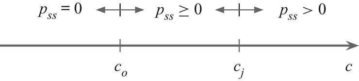
 $p_{ss}$ has not been considered in previous studies (Lee et al. Reference Lee, Low and Chiew2016; Chauchat et al. Reference Chauchat, Cheng, Nagel, Bonamy and Hsu2017; Lee & Huang Reference Lee and Huang2018; Si et al. Reference Si, Shi and Yu2018). Figure 1 presents
 $p_{ss}$ in different concentration regions. For
 $c<c_o$, the granular material cannot be packed randomly;
 $p_{ss}$ is zero. For
 $c_o \leq c < c_j$, the granular material flows or can be packed, and
 $p_{ss} \geq 0$. For
 $c\geq c_j$, the granular material behaves like a solid, suggesting
 $p_{ss}> 0$.
Static component of the solid pressure in the different concentration regions.

2.3. Solid stress
The shear stress tensor for the sediment phase is computed by
 \begin{equation} {\boldsymbol{\mathsf{T}}}^{s} = - (\tfrac{2}{3}\rho_{s}\nu_{s}\boldsymbol{\nabla} \boldsymbol{\cdot} \boldsymbol{u}^s ) {\boldsymbol{\mathsf{I}}} + 2 \rho_{s}\nu_{s} {\boldsymbol{\mathsf{D}}}^s, \end{equation}
where  $\nu _s$ is the viscosity of the solid phase. To consider the friction and dilatancy effects,
 $\nu _{s}$ is given by
 \begin{equation} \nu_{s}=\frac{p_{sd} \eta_d +p_{ss} \eta_s }{2\rho_s D^s} [1-\exp{(-2D^s/m)}], \end{equation}
where  $m$ is a constant with a small value (
 $m=10^{-5}$ is used here) and
 $\eta _{d/s}$ represents the dynamic/static friction coefficient. The regularisation scheme of Papanastasiou (Reference Papanastasiou1987) has been adopted in (2.13). As
 $m$ approaches zero, equation (2.13) is reduced to
 $\nu _{s}=(p_{sd} \eta _d +p_{ss} \eta _s )/(2\rho _s D^s)$, where
 $p_{sd}\eta _d+p_{ss}\eta _s$ is considered a yield stress. Physically, when
 $|{\boldsymbol{\mathsf{T}}}^s| < p_{sd}\eta _d+p_{ss}\eta _s$, the granular material does not yield and remains static. Numerically, the regularisation scheme treats the non-yielded granular material as a highly viscous fluid, which avoids the discontinuity problem near the yield point.
The formula of Trulsson et al. (Reference Trulsson, Andreotti and Claudin2012) is adopted to determine  $\eta _d$:
 \begin{equation} \eta_{d} = \eta_1+\frac{\eta_2-\eta_1}{1+I_o / I^{1/2}}, \end{equation}
where  $I_o=0.1$,
 $\eta _{1} = \tan \theta _s$ with angle of repose
 $\theta _s$,
 $\eta _{2}$ is the maximum friction coefficient and
 $I$ is a dimensionless parameter. The
 $\eta _{1}$ and
 $\eta _2$ values vary with different particle types. The dimensionless parameter
 $I$ is a combination of the viscous number
 $I_v$ and inertial number
 $I_i$:
 $I=I_v+aI_i^2$. The viscous number is the ratio of the viscous stress to the quasi-static shear stress associated with the weight (due to enduring contact) and is defined by
 $I_v=2\rho _f\nu _fD^s/cp_s$. The inertial number, defined by
 $I_i=2dD^s/\sqrt {cp_s/\rho _s}$, is the ratio of the inertial stress to the quasi-static stress. The formula of Trulsson et al. (Reference Trulsson, Andreotti and Claudin2012) considers the effects of both the particle inertia and fluid viscosity on the friction coefficient; other formulae consider either the particle inertia (Jop, Forterre & Pouliquen Reference Jop, Forterre and Pouliquen2006) or the fluid viscosity (Cassar et al. Reference Cassar, Nicolas and Pouliquen2005).
This study uses the following formula to determine  $\eta _s$:
 \begin{equation} \eta_s = \eta_1+\left(c-c_c\right)d_{p1}, \end{equation}
where  $c_c$ is the critical concentration and is determined by
 \begin{equation} c_c=p_{ss}/a_eE+c_j \end{equation}
without considering the dynamic effects on the critical concentration. The second term on the right-hand side of (2.15) accounts for the effect of the dilatancy angle, as in previous studies (Pailha & Pouliquen Reference Pailha and Pouliquen2009). When  $c$ is larger (smaller) than
 $c_c$, the dilatancy angle is positive (negative), thus increasing (decreasing) the friction coefficient. When
 $c$ is very small,
 $\eta _s$ becomes negative. In this case,
 $p_{ss}$ must be zero, so the negative friction force does not occur. Equation (2.14) does not incorporate the effect of the dilatancy angle to avoid the negative friction force.
2.4. Numerical scheme
The equations listed in § 2 are solved using OpenFOAM, an open-source computational fluid dynamics toolbox based on the finite-volume method (Jasak Reference Jasak2009). OpenFOAM supports three-dimensional (3-D) unstructured meshes and provides several discrete schemes and linear algebra solvers. There exists a challenge to solving those equations: an instability issue due to the sensitivity of the solid pressure to the concentration (see (2.7)). To address this issue, the numerical procedure proposed by Lee et al. (Reference Lee, Low and Chiew2016) is adopted, which is a combination of the PIMPLE scheme (OpenCFD 2014) and a prediction–correction scheme proposed by Lee, Huang & Chiew (Reference Lee, Huang and Chiew2015). The PIMPLE scheme is a combination of the ‘pressure implicit with splitting of operator’ and ‘semi-implicit method for pressure-linked equations’ schemes to determine the hydrodynamic pressure ( $p_f$). In the prediction–correction scheme proposed by Lee et al. (Reference Lee, Huang and Chiew2015), the discrete mass-balance equation for the sediment phase (2.3) is an advection–diffusion equation instead of an advection equation. The diffusion behaviour increases the numerical stability.
2.5. Comments
The physics behind the closures to compute  $p_s$ and
 ${\boldsymbol{\mathsf{T}}}^s$ corresponds to interactions in the granular mixture. The model parameters depend on the particle shape, friction and other properties. The present model is not limited to the submarine granular flows. With appropriate modifications, such as including the turbulence effect, the present model can be applied to simulate sediment transport in river and marine environments.
3. Simple shear flows of a dry granular material
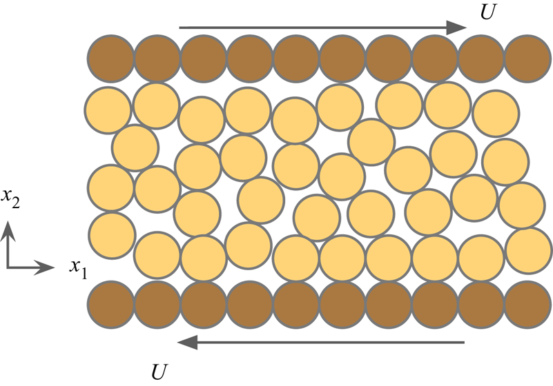
To examine the abilities of (2.9) to capture the solid pressure relaxation and shear-induced volume change, two tests are conducted concerning simple shear of a dry granular material with  $c>c_j$ (yielded amorphous solid), as presented in figure 2. In such flows, the granular material is sheared by the upper and lower plates with velocity
 $U$. The pore pressure is ignored in this section, and the strain rate is sufficiently small that
 $p_{sd}$ can be neglected. The flow fields are uniform in the
 $x_1$ direction. In the
 $x_2$ direction,
 $p_{ss}$,
 $c$ and
 $\partial u^s_1 / \partial x_2$ are uniform. Either the applied pressure on the plates or the volume between the two plates are fixed. The first test, with confined volume, is used to investigate the relaxation process. The other case, with confined pressure, is applied to examine the shear-induced volume change. The first test is less relevant with respect to other tests in the present study; however, it validates (2.9) directly.
Simple shear flows of a dry granular material.

3.1. Confined-volume test
For the confined-volume system, where  $u^s_2=0$, (2.9) reduces to
 \begin{equation} \frac{\partial p_{ss}}{\partial t}= c {d_{p1}} \frac{\partial u_1^s}{\partial x_2} (p_{ssc} - p_{ss}). \end{equation}
The solution to (3.1) is
 \begin{equation} p_{ss}(t) = p_{ssc} + [p_{ssc}-p_{ss}(0)]\exp \left(-c {d_{p_1}}\frac{\partial u_1^s}{\partial x_2}t\right). \end{equation}
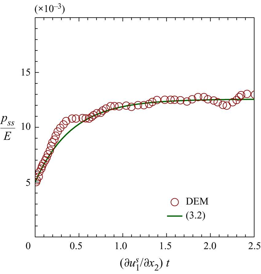
Equation (3.2) suggests an exponential decay of  $p_{ss}$ from
 $p_{ssi}$ to
 $p_{ssc}$, which is presented in figure 3 with
 $c=0.6$,
 $d_{p1}=4$,
 $p_{ssc}/E=1.26\times 10^{-2}$ and
 $p_{ss}/E=5\times 10^{-3}$. For validation, figure 3 also includes the DEM result of Sun & Sundaresan (Reference Sun and Sundaresan2011), which was obtained in the simple shear configuration with a sudden change in the shear direction. Strong particle rearrangement occurred when the shear velocity suddenly changed. Then, the particle arrangement approached another equilibrium state with the fabric tensor (associated with the inter-particle contact vector) approaching a constant. Figure 3 presents the DEM result close to the equilibrium state with a left shift by
 $(\partial u_1^s/\partial x_2) t = 2.5$. To the author's knowledge, there have been no DEM results of the solid pressure published for a planar shear flow with constant
 $U$. Referring to figure 3, (2.9) can properly reflect the relaxation process of
 $p_{ss}$. In reality, submarine granular flows are driven by gravity or water flows; in general, a submarine granular flow does not change its direction suddenly and (2.9) is applicable. For some cases with a sudden change in flow direction, (2.9) may be inapplicable; in those cases, more equations to describe the microstructural evolutions (Sun & Sundaresan Reference Sun and Sundaresan2011) should be solved.
Evolution of solid pressure for the confined-volume system.

3.2. Confined-pressure test
For the confined-pressure system, the shear-induced flow is not only in the  $x_1$ direction, but also in the
 $x_2$ direction, leading to a volume change. In this system, (2.9) is reduced to
 \begin{equation} \frac{\partial c}{\partial t}+\frac{d_{p1}}{ d_{p2}} \frac{\partial u_1^s}{\partial x_2} c (p_{ssc}-p_{ss}) =0. \end{equation}
Equation (2.3) has been used in (3.3). In this case,  $p_{ss}$ is constant and determines the critical concentration. By application of (2.10), (3.3) becomes
 \begin{equation} \frac{\partial c}{\partial t}+{d_{p1}}\frac{\partial u_1^s}{\partial x_2}c(c-c_{c}) =0. \end{equation}
Equation (3.4) suggests that  $c$ tends towards
 $c=c_c$. Equation (3.4) is identical to the theory of Roux & Radjai (Reference Roux, Radjai, Hermann, Hovi and Luding1997) describing the volume change:
 \begin{equation} \frac{\partial c}{\partial t}+ K \frac{\partial u^s_1}{\partial x_2}c(c - c_c)=0, \end{equation}
where  $K$ is a model parameter used in the linearisation of the dilatancy angle,
 $K(c - c_c)=\tan {\psi }$. A comparison of (3.4) and (3.5) suggests
 $K=d_{p1}$. Previous studies used
 $K=3.4$ (Pailha et al. Reference Pailha, Nicolas and Pouliquen2008) and
 $K=4.09$ (Pailha & Pouliquen Reference Pailha and Pouliquen2009). This study adopts
 $d_{p1}=K=4$.
The solution to (3.4) is
 \begin{equation} c(t)= \frac{c_{c}}{1+\dfrac{c_c-c(0)}{c(0)} \exp\left({- {d_{p1}} c_{c} \dfrac{\partial u_1^s}{\partial x_2} t}\right)}. \end{equation}
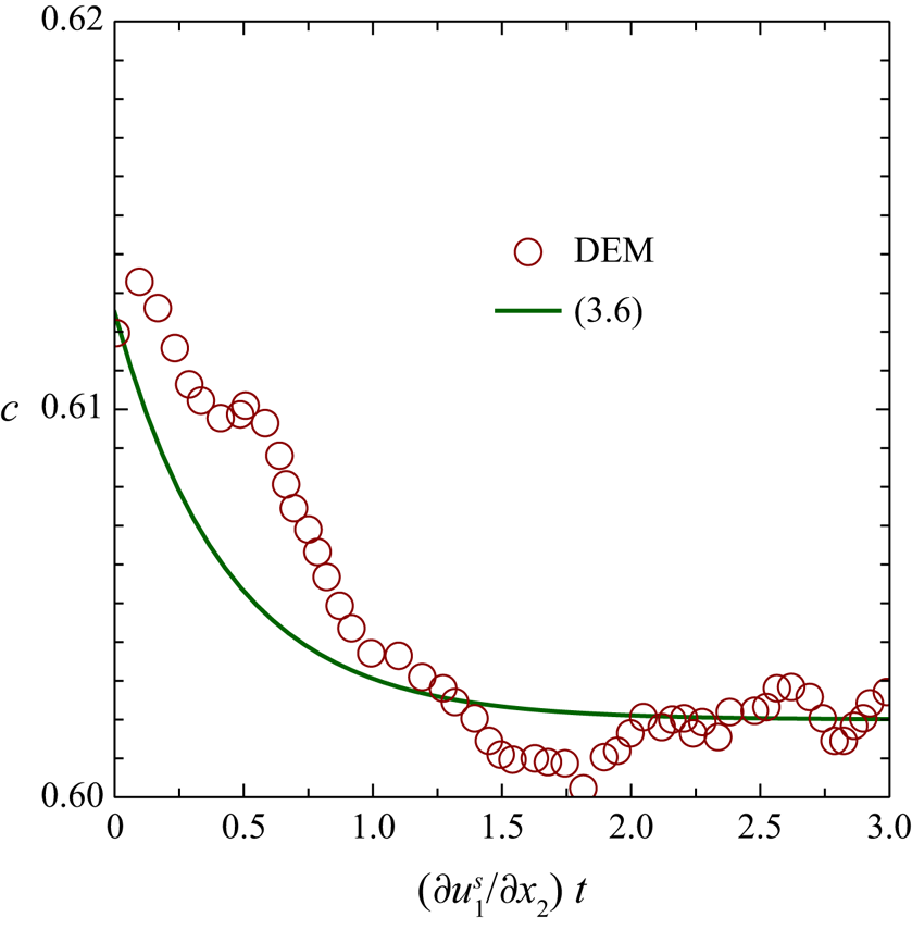
Figure 4 shows the evolution of the concentration for a densely packed (over-compacted) case. The DEM result of Sun & Sundaresan (Reference Sun and Sundaresan2011) with a steady shear is also superposed in figure 4 for comparison. It can be seen in figure 4 that (2.9) can effectively capture the shear-induced volume change in general. Nevertheless, there exist some discrepancies. For example, the DEM result shows an initial contraction behaviour (increasing  $c$), but the analytical result does not.
Evolution of concentration for the confined-pressure system.

3.3. Discussion
It has been shown in figures 3 and 4 that the evolution equation (2.9) can effectively describe the relaxation of the solid pressure and the shear-induced volume change in the quasi-static state. Elastic formulae (e.g. (2.10)) have one-to-one relationships between the static solid pressure and the concentration; hence, the elastic formulae cannot reflect the relaxation of the static solid pressure and volume change in plane-shear configurations.
Section 3.2 shows that the present evolution equation can be simplified to the theory of Roux & Radjai (Reference Roux, Radjai, Hermann, Hovi and Luding1997) (see (3.4) and (3.5)) in the extreme scenario with a fixed solid pressure (§ 3.1). The present evolution equation can also be applied to another extreme scenario with a fixed concentration but varying solid pressure; the theory of Roux & Radjai (Reference Roux, Radjai, Hermann, Hovi and Luding1997) cannot. Therefore, the present evolution equation has broader applicability than that of Roux & Radjai (Reference Roux, Radjai, Hermann, Hovi and Luding1997).
The evolution equation has certain limitations. For the densely packed granular material, a short-term contraction occurs before the dilatation (see figure 4). The evolution model, as well as the theory of Roux & Radjai (Reference Roux, Radjai, Hermann, Hovi and Luding1997), cannot capture this phenomena. Additionally, the evolution equation reflects a linear  $c$–
 $\tan \psi$ relationship across
 $c_c$ in the extreme scenario with a fixed solid pressure. Previous studies have usually focused on the densely packed granular material (Bolton Reference Bolton1986); the contraction behaviour for the loose-packing case is not well understood. The
 $c$–
 $\tan \psi$ relationship might be more complex.
4. Initiation of submarine granular flow
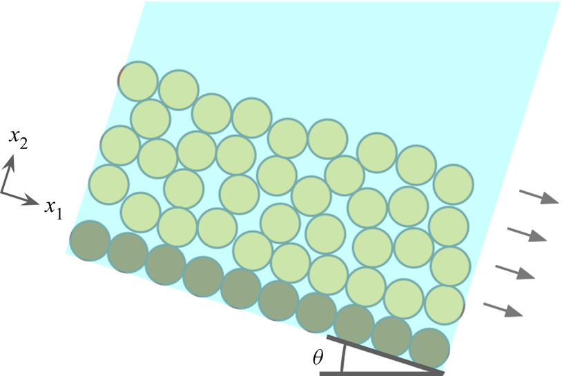
This section further examines the ability of the present model to simulate the initiation of a submarine granular flow, as shown in figure 5. This case is a benchmark to study the pore-pressure feedback (Pailha et al. Reference Pailha, Nicolas and Pouliquen2008), which involves coupling between the particle and fluid dynamics. The particle dynamics, fluid dynamics and their interactions should be described in a model so that good simulation results can be obtained for this case. A layer of glass particles with height of 6 cm on slopes with incline angles of  $\theta = 28^\circ$ and
 $30^\circ$ is considered. The particles with
 $d=0.16$ mm and
 $\rho _s = 2500$ kg m
 $^{-3}$ are immersed in the fluid with
 $\rho _f = 1016$ kg m
 $^{-3}$ and
 $\nu _f=9.5516\times 10^{-6} \ {\rm m}^{2} \ {\rm s}^{-1}$. In the simulations,
 $\eta _1=0.41$ and
 $\eta _2=0.62$ are used. Young's modulus of
 $E=10^6$ Pa is taken, which is less than the value of
 $E=10^{10}$ Pa for glass; using an excessively high
 $E$ causes numerical instability. Concerning the two parameters affecting
 $\tau _p$ (
 $a_E$ and
 $b_E$; see appendix B),
 $a_E=780$ and
 $b_E=1.8$ are used. In the
 $x_1$ direction, only one grid is used, and a periodic boundary condition is imposed. In the
 $x_2$ direction, uniform grids of length
 ${\rm \Delta} x = 0.2$ cm are used;
 ${\rm \Delta} x = 0.2$ and
 ${\rm \Delta} x = 0.1$ cm yields only 2.7 % difference in the surface velocity for
 $c_{init}=0.576$. The time step of
 ${\rm \Delta} t = 10^{-5}$ is adopted. No-slip conditions for both phases are imposed on the boundary. In the simulations, mass conservation is satisfied; the relative variation in the total sediment volume is observed to be within
 $10^{-6}$.
Initiation of underwater granular avalanche.

4.1. Validation
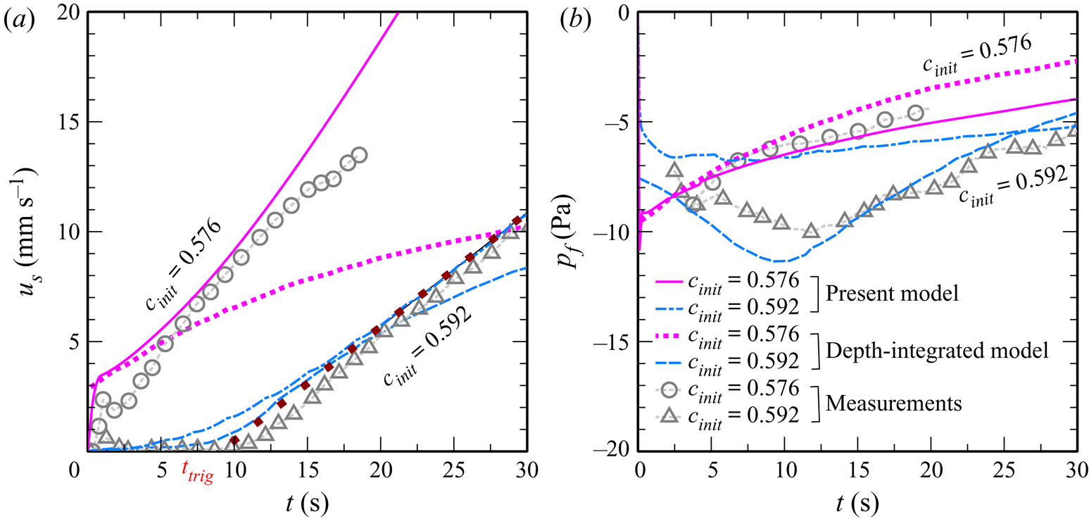
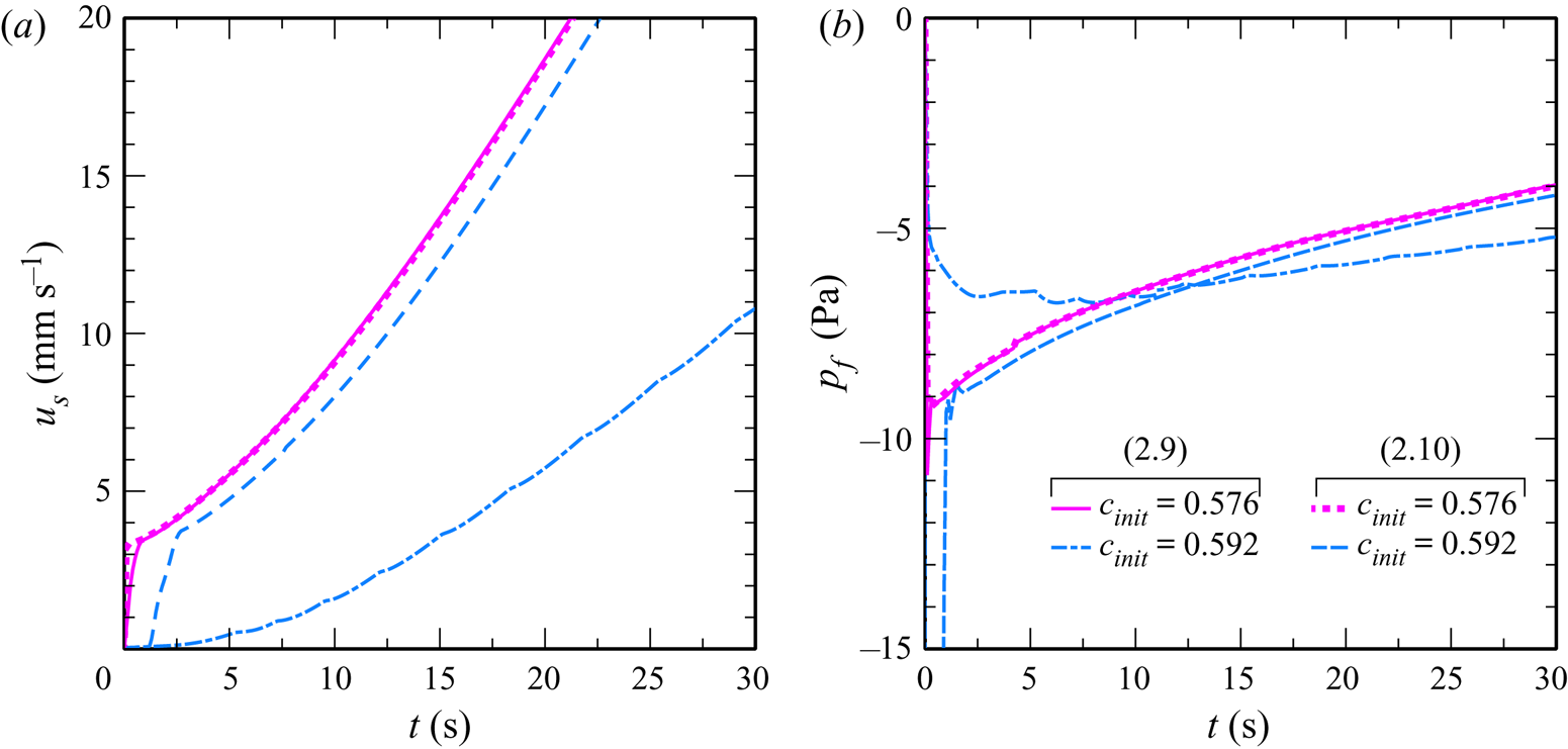
Figure 6(a) presents a comparison between the top-surface velocities,  $u_s$, obtained using three different approaches: (i) a physical model (Pailha et al. Reference Pailha, Nicolas and Pouliquen2008), (ii) the present numerical model, and (iii) a previous depth-integrated model (Bouchut et al. Reference Bouchut, Fernández-Nieto, Mangeney and Narbona-Reina2016). The comparisons of basal pore pressures obtained using these approaches are shown in figure 6(b). The initial concentrations of
 $c_{init}=0.576$ and
 $c_{init}=0.592$ are used. The incline angle (
 $\theta$) is
 $28^\circ$. The top-surface velocity is defined at the location with
 $c=0.5$ in the present simulation. The physical model (Pailha et al. Reference Pailha, Nicolas and Pouliquen2008) uses a box filled with liquid and particles; the submarine granular flows are initiated by suddenly tilting the box. The effects of the ends of the box and the sudden tilt are not considered in either numerical model.
Comparison of the top-surface velocities and basal pore pressures between different approaches. The solid line represents the present numerical results, the circles represent the experimental results (Pailha et al. Reference Pailha, Nicolas and Pouliquen2008), and the dashed line represents the numerical results using two-layer models (Bouchut et al. Reference Bouchut, Fernández-Nieto, Mangeney and Narbona-Reina2016). The dotted line is the line of best fit to the computed  $u_s$ in the acceleration stage using the present model.

Referring to figure 6, the loose case ( $c_{init} = 0.576$) and dense case (
 $c_{init} = 0.592$) have different flow features. For the loose case (
 $c_{init} = 0.576$), the particles have an initial rapid acceleration (
 $t<1$ s for the measured results), and then the acceleration becomes milder (
 $t>1$ s); the pore pressure increases in the mild acceleration stage. For the dense case (
 $c_{init} = 0.592$), the sediment dynamics are characterised by a creeping motion (
 $t<11$ s for the measured results), followed by an acceleration motion (
 $t>11$ s); the pore pressure decreases in the creeping stage, then increases in the acceleration stage. The computed top-surface velocities and basal pore pressures using the present model and the depth-integrated model (Bouchut et al. Reference Bouchut, Fernández-Nieto, Mangeney and Narbona-Reina2016) generally agree with the experimental ones, but some inconsistencies exist. The negative pore pressure computed by the present model is lower than that measured for the dense case. The depth-integrated model underestimates the acceleration in the mild acceleration stage of the loose case. The boundary between the creep and acceleration stages is clear in the measured results, but not in both computed results.
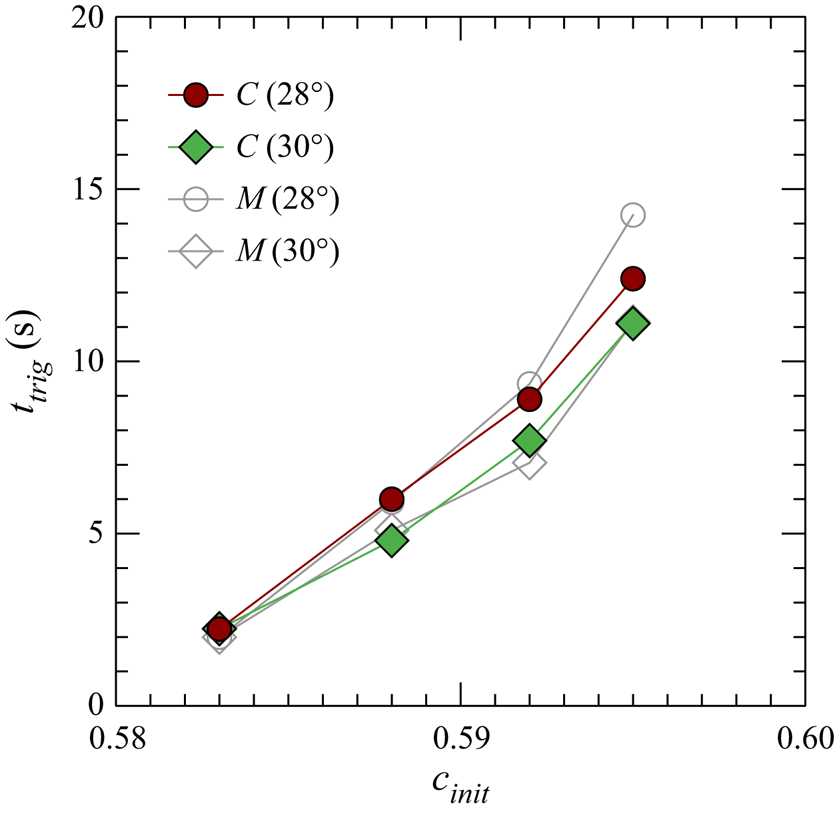
To compare the experiments and the present model more systematically, the computed triggering time (time delay or creeping-motion duration),  $t_{trig}$, and the measured ones (Pailha et al. Reference Pailha, Nicolas and Pouliquen2008) are plotted in figure 7 against different
 $\theta$ and
 $c_{init}$. The triggering time is determined by the intersection between the fitting line to
 $u_s$ in the acceleration stage and the time axis. Both the measured and computed results reveal (i) a positive relationship between
 $t_{trig}$ and
 $c_{init}$ and (ii) the negative effect of
 $\theta$ on
 $t_{trig}$. The reasonable, quantitative agreement between the computed
 $t_{trig}$ and the measured one is observed in figure 7, indicating that the present model can capture the dynamics of the initiation of submarine granular flows.
Triggering time versus  $c_{init}$ for different
 $\theta$. The closed symbols represent the numerical results and the open ones the measured results (Pailha et al. Reference Pailha, Nicolas and Pouliquen2008).

4.2. Depth-resolving flow fields
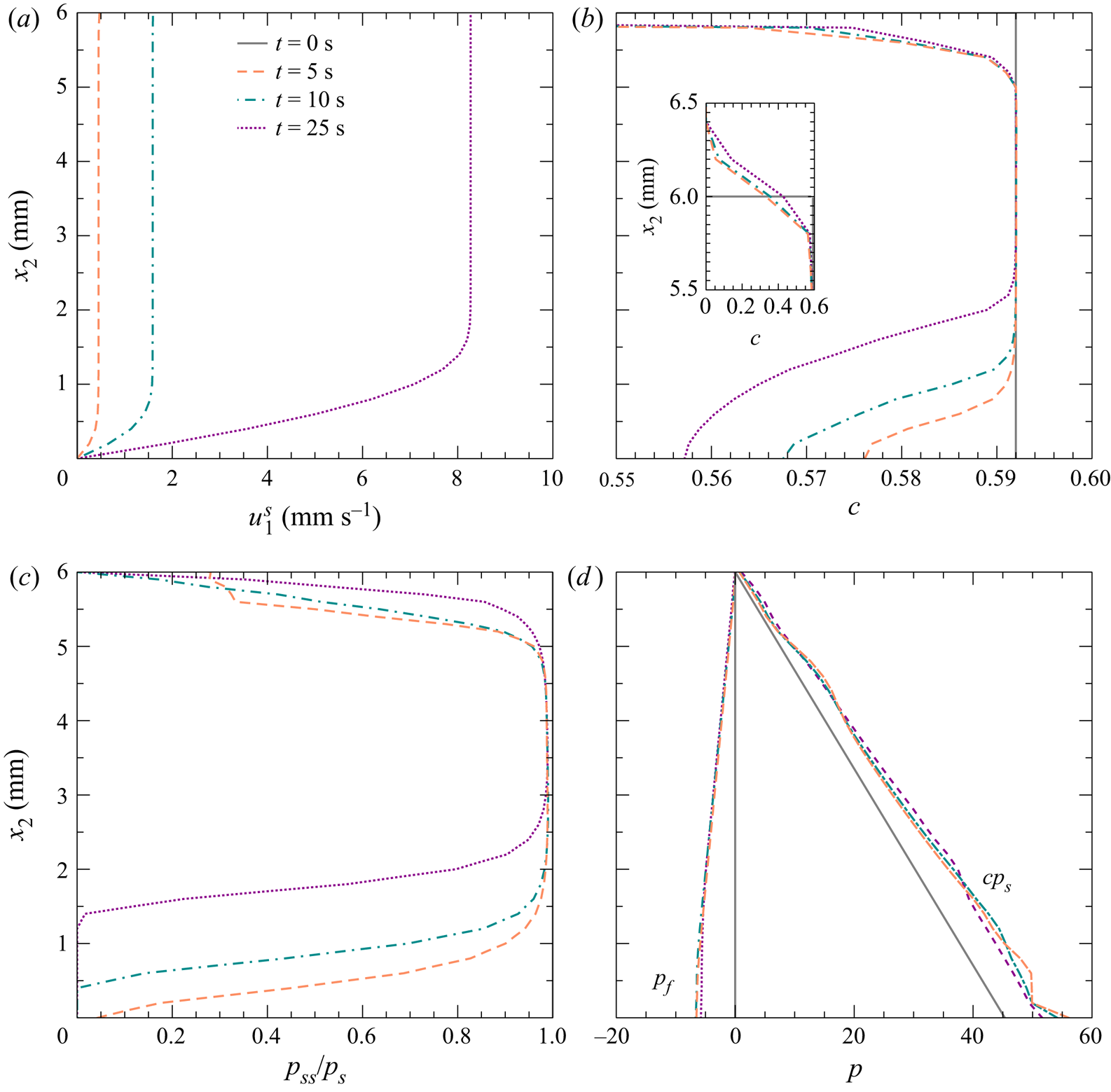
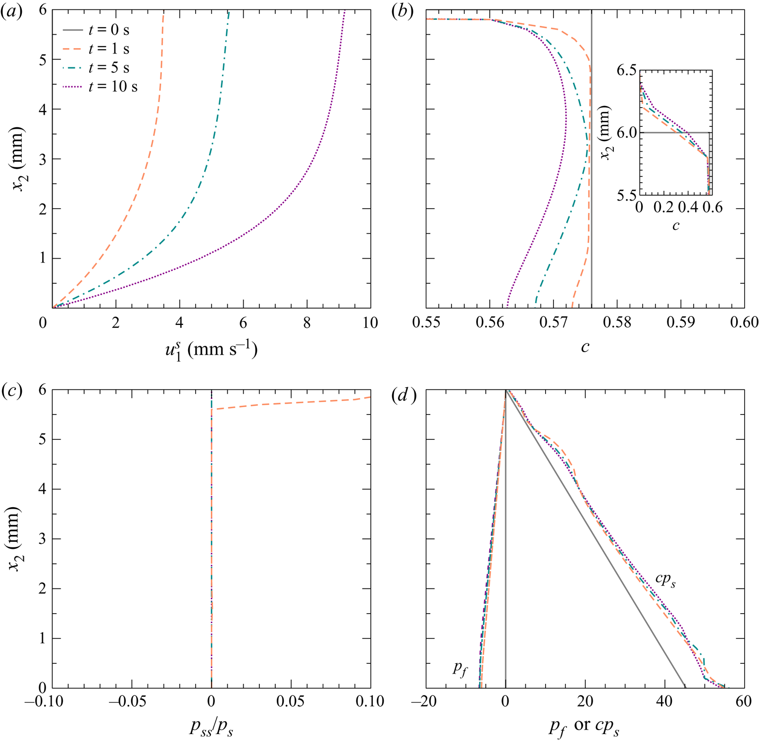
To further examine the computed submarine granular flows, the profiles of the velocity, the concentration, the ratio of static solid pressure to the solid pressure, and the pressures for both phases are shown in figures 8 and 9 for the dense and loose cases, respectively. The flows presented in figures 8 and 9 are in the transition state. The two cases have similar profiles when the flows have fully developed, which are not shown in figures 8 and 9.
(a) Computed velocity, (b) concentration, (c) ratio of the static component to the total solid pressure, and (d) pore pressure at  $t= 0$, 5, 10 and 25 s for the dense case with
 $c_{init} = 0.592$ and
 $\theta =28^\circ$. The inset in panel (b) is an enlarged view of concentration profiles around
 $x_2=6$ mm.

(a) Computed velocity, (b) concentration, (c) ratio of the static component to the total solid pressure, and (d) pore pressure at  $t= 0$, 1, 5 and 10 s for the loose case with
 $c_{init} = 0.576$ and
 $\theta =28^\circ$. The inset in panel (b) is an enlarged view of concentration profiles around
 $x_2=6$ mm.

The velocity profiles in both cases are significantly different: a plug flow over a shear band in the dense case (figure 8a) and the shear distributed over the flow in the loose case (figure 9a). According to (2.15), the dense case has  $\eta _s \approx 0.474$, but the loose case has
 $\eta _s \approx 0.41$ at
 $t=0$ s. The higher friction coefficient of the dense case causes a lower dispersion rate of shear compared to that of the loose case. Therefore, the plug region exists after
 $t=25$ s in the dense case, but the shear has been distributed over the flow before
 $t=1$ s in the loose case.
In both cases, the dilatation occurs in the shear regions near the beds (figures 8b and 9b). The sign of  $c_{init}-c_c$ suggests the direction of the volume change. According to (2.16),
 $c_c$ should be slightly larger than
 $c_j=0.576$ due to gravity and the very large value of
 $E$. Dilatation is expected for the dense case with
 $c_{init}=0.592$ (
 $c_{init}-c_c>0$) and contraction is expected for the loose case with
 $c_{init}=0.576$ (
 $c_{init}-c_c<0$). However, the numerical result reveals dilatation in the loose case. In this study,
 $c_c$ is computed without considering its dynamic effects on
 $c_c$. In the loose case, the static solid pressure (
 $p_{ss}$) disappears rapidly (see figure 9c); the shear can cause the dynamic solid pressure (
 $p_{sd}$) to increase locally (see (2.6) and (2.7)) and is responsible for the dilatation in the loose case. In the dense case, the static and dynamic solid pressures suggest dilatation. Because of the dilatation in both cases, the downward buoyancy (the positive pressure gradient of the fluid phase in figure 8d) at
 $t>0$ s is observed in both cases, increasing the solid pressure and friction compared to those at
 $t=0$ s.
4.3. Shear-induced volume change
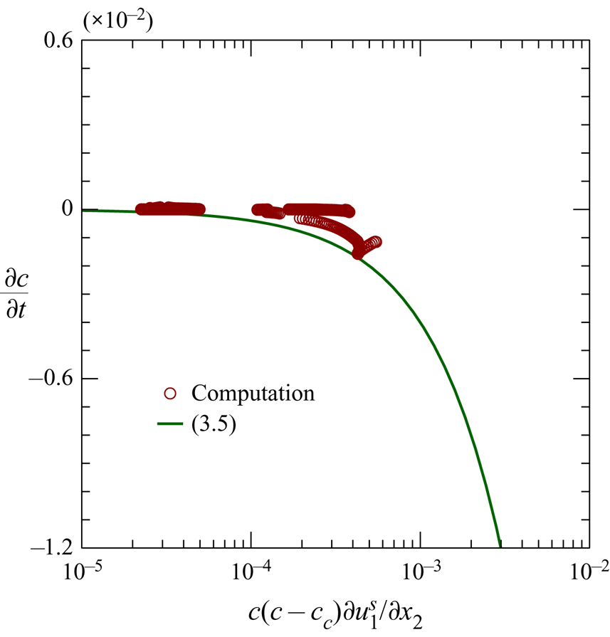
Figure 10 shows the rate of concentration change ( $\partial c / \partial t$) against
 $c (c-c_c)\partial u^s_1/\partial x_2$ obtained in the simulations. Only the result of the dense case is presented, in which the static effect inducing the volume change is significant. The theory of Roux & Radjai (Reference Roux, Radjai, Hermann, Hovi and Luding1997) is also included in figure 10 for comparison. It can be seen in figure 10 that the magnitude of the concentration change rate,
 $|\partial c/\partial t|$, obtained in the present simulation is smaller than that predicted by (3.5). The theory of Roux & Radjai (Reference Roux, Radjai, Hermann, Hovi and Luding1997) is applicable for the extreme scenario with variable concentration and fixed solid pressure. In the dense case, the concentration and solid pressure are variable; therefore, the rate of concentration change determined by the present model is smaller than that found using (3.5), as observed in figure 10.
Rate of concentration change induced by shear for the dense case  $c_{init} = 0.592$ and
 $\theta =28^\circ$.

4.4. Comparison with the flows computed using the elastic formula
To understand how much better the evolution equation is than the elastic formula to compute the static solid pressure ( $p_{ss}$), figure 11 compares the computed top-surface velocities and the basal pore pressures using the evolution equation (2.9) and elastic formula (2.10). When using the elastic formula,
 $p_{ss}=p_{ssc}$ is taken. The primary difference between the two approaches is the relaxation of pressure. It can be seen in figure 11 that using the elastic formula yields similar results (including top-surface velocities and the basal pore pressure) to using the evolution equation for the loose case but very different results for the dense case. For the loose case, the contribution of the static solid pressure disappears quickly (presented in § 4.2), leading to similar results using the two approaches. For the dense case, using the elastic formula yields a sudden dilatation (
 $c\approx 0.576$ through the flow at
 $t=1$) to reflect the excessive static solid pressure, leading to huge negative pore pressure. Creep motion obtained using the elastic formula is short due to the rapid dissipation of pore pressure. After the sudden dilatation produced by the elastic formula, the material (originally in the dense state) becomes loose with
 $c\approx 0.576$. Therefore, using the elastic formula provides similar results for the dense and loose cases, except for the creep motion of the dense case.


4.5. Discussion
The present model predicts an unclear boundary between the creep motion and acceleration, and the negative pore pressure is underestimated in the dense case. Considering the non-local effect in the evolution equation may provide a clearer boundary and larger negative pore pressure more correctly. The non-local effect is due to the stress fluctuations helping the granular material to yield (Pouliquen & Forterre Reference Pouliquen and Forterre2009). Considering the non-local effect might broaden the dilatation area, increasing the negative pore pressure and friction; the resultant creep motion can be slower than the original (without considering the non-local effect). The non-local effect is not well understood at present, and is not included in the present model. The depth-integrated model of Bouchut et al. (Reference Bouchut, Fernández-Nieto, Mangeney and Narbona-Reina2016) does not include the non-local effect, but it can predict the top-surface velocity and basal pore pressure for the dense case. The model determines the depth-averaged properties based on empirical formulae; it may contain the non-local effect through these empirical formulae.
In this study,  $E$ and
 $a_{ei}$ are tuning parameters. Sensitive analyses of the top-surface velocity and basal pore pressure of the two parameters can be found in appendix C. Sensitive analysis of
 $a_E$ and
 $b_E$ is included in appendix C; the two parameters determine the interfacial forces and may play significant roles in the pore-pressure feedback.
5. Collapse of submerged granular column
Rondon et al. (Reference Rondon, Pouliquen and Aussillous2011) performed the experiments on the collapse of submerged granular columns using a 70 cm long, 15 cm wide and 30 cm high perspex tank filled with liquid. A vertical wall was positioned on an end of the tank to create a reservoir for the granular material. A collapse is initiated by removing the vertical wall. They used glass beads with  $d = 0.225$ mm,
 $\rho _s = 2500$ kg m
 $^{-3}$ and a fluid with
 $\rho _f = 1010 \ {\rm kg} \ {\rm m}^{-3}$, as well as
 $\nu _f=1.2\times 10^{-5} \ {\rm m}^{2} \ {\rm s}^{-1}$, in their experiments. They reported the collapse processes of a densely packed column and a loosely packed column. The former is 6 cm wide and 4.2 cm high with the initial concentration of
 $c_{init}=0.6$; the latter, with
 $c_{init}=0.55$, is 6 cm wide and 4.2 cm high. High/low pore pressure was experimentally observed at the centre of the bottom of the loosely/densely packed column. The loosely packed column has a more rapid collapse process than the densely packed one. These phenomena are typical results of the pore-pressure feedback (Rondon et al. Reference Rondon, Pouliquen and Aussillous2011).
This section applies the present model to reproduce the experiments of Rondon et al. (Reference Rondon, Pouliquen and Aussillous2011). In the simulations,  $\eta _1=0.41$,
 $\eta _2=0.62$,
 $E=10^6$ Pa,
 $a_E=1500$ and
 $b_E=1.8$ are used. The rectangular computational domain is 0.4 m long and 0.3 m high. A uniform grid with square cells (
 ${\rm \Delta} x = 1$ mm) is adopted. The convergence tests are performed using the loose case. A comparison of the flow-front location obtained using
 ${\rm \Delta} x =1$ mm and
 ${\rm \Delta} x = 2$ mm shows that the difference was less than 0.1 %. No-slip conditions for both phases are imposed on the bottom and two sides. On the top,
 $p=0$ Pa is taken and the fluid velocity is determined according to the mass balance. In all numerical simulations, the Courant–Friedrichs–Lewy (CFL) number did not exceed 0.1. In high-concentration regions (
 $c > 0.55$), the CFL number used in the simulations was less than 0.005. The relative variation in the total sediment volume is within
 $2\times 10^{-5}$ in the simulations.
5.1. Validation
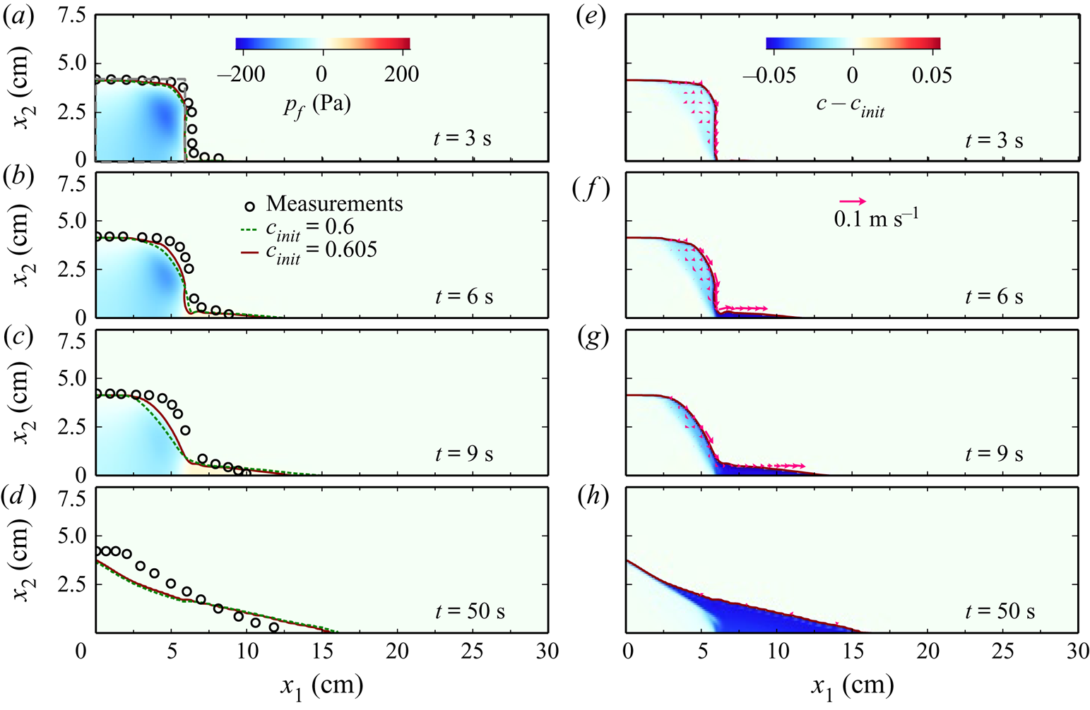
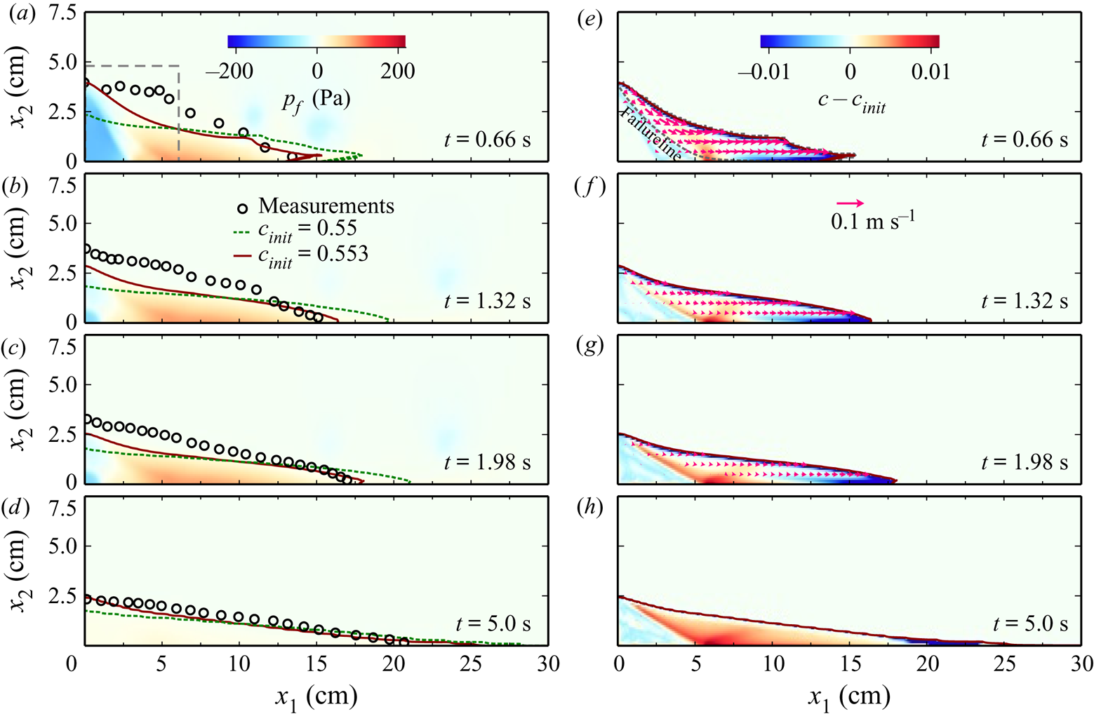
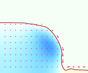
Figures 12 and 13 present the computed collapse process of the densely and loosely packed columns, respectively. The pressure fields, the shape of the columns (contour lines of  $c=0.5$), the velocity fields of the solid phase, and the concentration deviation from the initial concentration (
 $c-c_{init}$) are included in figures 12 and 13. The concentration deviation can be used to evaluate the dilatation (or contraction) that occurs in the sliding part in the early stage, but not in the deposition part in the final stage. Owing to the uncertainty in measuring the initial concentration (approximately 0.9 %) (Rondon et al. Reference Rondon, Pouliquen and Aussillous2011),
 $c_{init} = 0.6$ and 0.605 are used for the dense case;
 $c_{init} = 0.55$ and 0.553 are applied for the loose case. For the simulation results with
 $c_{init}=0.6$ and
 $c_{init}=0.55$, only the shapes of the columns at different instants are presented. The measured results by Rondon et al. (Reference Rondon, Pouliquen and Aussillous2011) are superposed in these two figures for comparison. The computed and measured basal pore pressures at
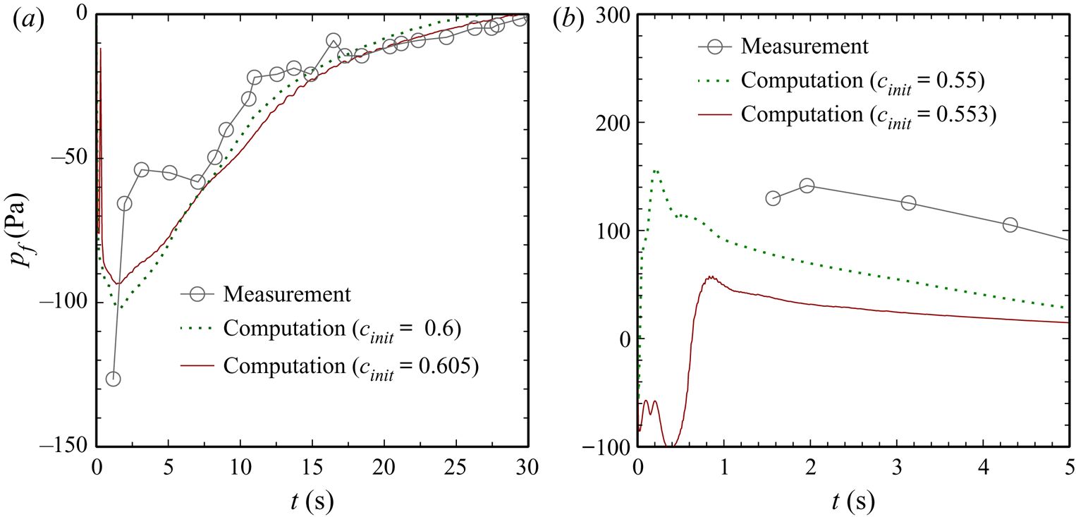
 $x_1 = 3$ cm are plotted in figure 14.
Sequences of the collapsing process for the densely packed column. The lines present contours of  $c=0.5$ for different
 $c_{init}$. The colour maps present the pore pressure (a–d) and the concentration deviating from
 $c_{init}$ (e–h) for
 $c_{init}=0.605$. The arrow, applying to (e–h), shows the solid velocity. The circles in (a–d) are experimental data from Rondon et al. (Reference Rondon, Pouliquen and Aussillous2011).

Sequences of the collapsing process for the loosely packed column. The lines present contours of  $c=0.5$ for different
 $c_{init}$. The colour maps present the pore pressure (a–d) and the concentration deviating from
 $c_{init}$ (e–h) for
 $c_{init}=0.553$. The arrow, applying to (e–h), shows the solid velocity. The circles in (a–d) are experimental data from Rondon et al. (Reference Rondon, Pouliquen and Aussillous2011).

Basal pore pressure at  $x_1=3$ cm for the loosely packed column (a) and the densely packed column (b).

A breaching process can be identified in figure 12 for the densely packed column, where the particles are spalled near the vertical face and the front of the column retreats slowly (Houssais & Jerolmack Reference Houssais and Jerolmack2017). The released particles move along the surface of the column and are finally deposited at the front of the column. The moving mass (e.g. the upper right corner at  $t=3$ s) goes through a dilatation process (
 $c-c_{init} < 0$) initially. The negative pore pressure is observed in the column, and its maximum occurs in the moving mass within
 $t=3$–
 $6$ s. The negative pore pressure dissipates completely before
 $t=50$ s. The computed results are consistent with the measured ones, including the shape (figure 12) and basal pore pressure (figure 14).
Figure 13 displays a slumping process for the loose case, where a granular mass (in the upper right part) slides down along a concave-upward failure surface (the isovalue line of  $|\boldsymbol {u}^s| = 0.5$ cm s
 $^{-1}$). At
 $t=0.66$ s, the moving mass, over the failure line, generally contracts with high pore pressure inside. Because the moving mass leaves the column, the failure line (the interface between the moving and non-moving parts) has lower
 $c$ than
 $c_{init}$. In other words, dilatation occurs along the failure line, leading to negative pore pressure there. Overall, the computed results with
 $c_{init}=0.553$ are consistent with the measured ones. For the loose case, the computed pore pressure with
 $c_{init}=0.553$ is smaller than the measured one (figure 14), but they are still of the same order of magnitude. It is noted that the experiments used a gate lifting upwards to initiate the collapse, which has a strong effect in the early stage of collapse (Ionescu, Mangeney & Roche Reference Ionescu, Mangeney and Roche2015). The gate effect is not considered in the computations, which may be the main reason for the minor discrepancy between the computed and measured results.
Previous studies (Rondon et al. Reference Rondon, Pouliquen and Aussillous2011) indicate that the initial concentration has important effects on the collapse due to shear-induced volume change and the resultant pore-pressure feedback. The present model can produce the collapse process for the densely and loosely packed columns with reasonable accuracy, including the shape and pore pressure; this suggests that the present model can effectively capture the submarine collapses.
It can be seen in figures 12–14 that the results including the collapse process and pore pressure are sensitive to  $c_{init}$ for the loose case but not for the dense case. Considering the loose case where
 $c_{init}$ is close to
 $c_o$ (random loose packing), the concentration near the failure line decreases. When
 $c$ becomes lower than
 $c_o$, the column loses support from the particle contact. The value of
 $c_{init}-c_o$ determines when the column loses support. Therefore, the collapse process is sensitive to
 $c_{init}$ for the loose case. The third term on the right-hand side of (2.9) reflects the loss of the support from the particle contacts when
 $c$ suddenly drops below
 $c_o$. For the dense case,
 $c_{init}$ is far from
 $c_o$; the sudden drop of
 $c$ to below
 $c_o$ does not usually occur. The collapse process is not sensitive to
 $c_{init}$ for the dense case.
5.2. Comparison with the collapses computed using the elastic formula
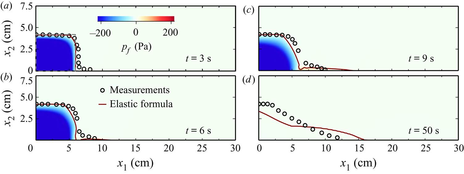
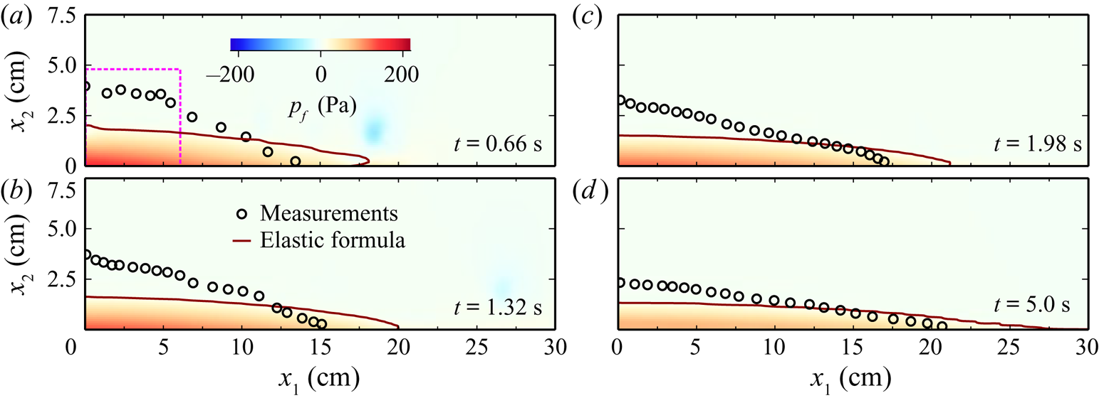
This section compares the collapse processes computed using the evolution equation (2.9) and elastic formula (2.10) to determine the static solid pressure. Figures 15 and 16 present the computed collapse processes of the dense and the loose cases, respectively, using the elastic formula. It is remarked that the colour is saturated for  $|p_f| > 220$ Pa in the figures. The absolute value of the negative pore pressure in figure 15 is much larger than 220.
Computed collapse of a dense column using (a) the evolution equation and (b) the elastic formula at  $t = 3$, 6, 9 and 50 s.

Computed collapse of a loose column using (a) the evolution equation and (b) the elastic formula at  $t = 0.66$, 1.32, 1.98 and 5.0 s.

Concerning the densely packed column, a comparison of figures 12 and 15 shows that using the evolution equation and using the elastic formula give very similar results in the evolution of column shapes. The velocity distributions obtained using these two approaches are also similar (the velocity using the elastic formula is not shown here). A significant difference exists in the pore pressure. Using the elastic formula yields a decrease in the pore pressure towards the interior of the column; this is due to the elastic effect and the overly rapid dilatation that occurs not only in the moving part (upper right corner), but also in the non-moving part. The concentration at the centre of the column ( $x_1=3$ and
 $x_2=2.1$ cm) changes from 0.605 to 0.593 within
 $t\leq 3$ s using the elastic formula. Because the centre of the column is not sheared before
 $t=3$, the concentration should not change. Using the evolution equation yields unchanged concentration at the centre of the column at
 $t\leq 3$ s. In addition to the pressure distribution, using the elastic formula also gives an unreasonable amount of pore pressure. The absolute value of pore pressure can exceed the measured one by over an order of magnitude. The computed basal pressure at
 $x_1=3$ cm using the elastic formula is
 $-$833 Pa at
 $t = 3$ s, but the measured one is
 $-$30 Pa.
For the loosely packed column, using the elastic formula yields more rapid collapse than the evolution equation; additionally, the former yields a shallower deposition than the latter (see figures 13 and 16). Since  $c_{init}=0.553$ is lower than
 $c_j=0.576$, the static solid pressure of
 $p_{ss}=0$ is obtained by using the elastic formula at
 $t=0$ s, and then the particles inside the column fall until the buoyancy or solid pressure force is sufficiently large to support these particles.
The previous study of Lee & Huang (Reference Lee and Huang2018) adopted an elastic formula to simulate the collapse of the dense and the loose cases. As in the present study, the elastic formula results in an unreasonable value of the negative pore pressure inside the densely packed column. For the loose case, the study of Lee & Huang (Reference Lee and Huang2018) using the elastic formula yields a reasonable pore pressure and collapse process, because  $c_{init}>c_j$ is adopted such that the static solid pressure force can support the column.
It can be concluded that the elastic formula can provide reasonable collapse for loosely packed columns by adjusting the value of  $c_{init}$ or
 $c_j$. However, the elastic formula cannot provide the correct pore pressure in densely packed columns. The evolution equation can provide a reasonable collapse process, including the shape evolution and pore pressure, for both cases.
6. Conclusions
The shear-induced volume change and the resultant pore-pressure feedback are two important issues that need to be addressed when using Eulerian–Eulerian two-phase models to simulate submarine granular flows. This study introduces a new evolution equation to determine the static solid pressure ( $p_{ss}$), considering the relaxation process of
 $p_{ss}$, the change in
 $p_{ss}$ caused by compression, and the change in
 $p_{ss}$ due to loss of inter-particle contacts. The evolution equation can produce the same relaxation process of
 $p_{ss}$ as the DEM simulation (Sun & Sundaresan Reference Sun and Sundaresan2011) in the condition of weak particle rearrangement. Analytically, the shear-induced volume change can be captured well by the evolution equation together with the linear relationship between
 $p_{ss}$ and the critical concentration (Sun & Sundaresan Reference Sun and Sundaresan2011). The evolution equation can be reduced to the theory of Roux & Radjai (Reference Roux, Radjai, Hermann, Hovi and Luding1997) in a plane-shear geometry with a constant confined pressure. The evolution equation is applicable to plane-shear cases with a fixed volume, whereas the theory of Roux & Radjai (Reference Roux, Radjai, Hermann, Hovi and Luding1997) is not.
This evolution equation allows the two-phase model to reproduce two benchmark cases related to pore-pressure feedback: the initiation of submarine granular flows and the collapse of submerged granular columns. The numerical results reveal reasonable time delay of initiating submarine granular flows and different collapse process for differently packed columns, which are important features that result from the pore-pressure feedback. The present work also compares the two cases obtained using the evolution equation and elastic formula to determine  $p_{ss}$. Using the evolution equation can provide reasonable results for both loose and dense cases, but the elastic formula is effective for loose cases only.
Finally, the proposed two-phase model is not limited to submarine granular flows. Further, by incorporating suitable modifications, the model can be applied to other solid–liquid flow problems, such as sediment transport in river and marine environments. The model was tested according to two-dimensional benchmarks, but it can be applied to 3-D cases without any modification. A possible scope for future work is to investigate submarine landslides with 3-D complex bathymetry.
Acknowledgements
This work is supported by the Ministry of Science and Technology, Taiwan, under grant MOST 109-2636-E-110-008 (Young Scholar Fellowship Program).
Declaration of interests
The author reports no conflict of interest.
Appendix A. Fluid stress
This study does not consider the turbulent motion of fluids, and the Newtonian fluid model is assumed. Accordingly,  ${\boldsymbol{\mathsf{T}}}^f$ is given by
 \begin{equation} {\boldsymbol{\mathsf{T}}}^{f} = - (\tfrac{2}{3}\rho_{f}\nu_{fv}\boldsymbol{\nabla} \boldsymbol{\cdot} \boldsymbol{u}^f ){\boldsymbol{\mathsf{I}}} + 2 \rho_{f}\nu_{fv} {\boldsymbol{\mathsf{D}}}^f, \end{equation}
where  $\nu _{fv}$ is the kinematic viscosity and
 ${\boldsymbol{\mathsf{D}}}^f = [\boldsymbol {\nabla } \boldsymbol {u}^f + (\boldsymbol {\nabla } \boldsymbol {u}^f)^{\textrm {T}}]/2$.
Appendix B. Particle response time
This study adopts the formula of Lee & Huang (Reference Lee and Huang2018) to determine the particle response time:
 \begin{equation} \tau_{p} = \left\{ \begin{array}{@{}ll} \displaystyle \dfrac{\rho_{s}}{\rho_{f}} \dfrac{d^2}{\nu_{fv}} \dfrac{(1-c)^{n-3}[\max(1-c/c_j,0)]^{c_{j} }}{18+({4.5}/{(1+\sqrt{Re_p})}+0.3) Re_p}, & \text{for } c < c_r, \\ \displaystyle\dfrac{\rho_{s}d^2}{\rho_{f} \nu_{fv}} \dfrac{1}{a_{E} c^{2} + b_{E} Re_{p}}, & \text{for } c \geq c_r , \end{array} \right. \end{equation}
where  $a_E$,
 $b_E$ and
 $n$ are the model parameters;
 $c_j$ is the concentration at the jamming point;
 $c_r$ is the concentration at the intercept point of the two equations in (B 1); and
 $Re_p=|\boldsymbol {u}^s-\boldsymbol {u}^f| d/\nu _{fv}$. The parameters
 $a_E$ and
 $b_E$ depend on the particle shape and particle compositions,
 $a_E$ can vary from 780 to 5000 or more, and
 $b_E$ can vary from 1.8 to 3.6 or more (Burcharth & Andersen Reference Burcharth and Andersen1995; Higuera, Lara & Losada Reference Higuera, Lara and Losada2014). The parameter
 $n$ is given by
 \begin{equation} n = \left\{ \begin{array}{@{}ll} 4.65, & Re_{s}<0.2, \\ 4.4Re_{s}^{-0.33}, & 0.2\le Re_{s}<1, \\ 4.4Re_{s}^{-0.1}, & 1\le Re_{s } < 500, \\ 2.4, & 500 \le Re_{s} , \end{array} \right. \end{equation}
where  $Re_s =w_s d/\nu _f$ with
 $w_s$ the terminal velocity of a single particle. Equation (B 1) combines the formula of Richardson & Zaki (Reference Richardson and Zaki1954) for low-concentration cases and that of Engelund (Reference Engelund1953) for high-concentration cases.
Appendix C. Sensitivity analyses
Sensitivity analyses are performed to examine the sensitivity of the top-surface velocity and basal pore pressure (as discussed in § 4) with respect to  $E$,
 $a_{ei}$,
 $a_{E}$ and
 $b_{E}$. The results obtained at the acceleration stage (
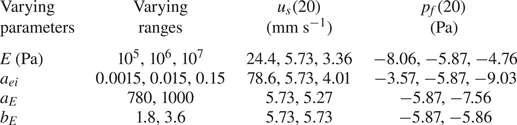
 $t=20$ s) for the dense (
 $c_{init}=0.592$) case are listed in table 1. In this study,
 $E=10^6$ Pa is adopted, which is much smaller than
 $E=10^9$ Pa for glass owing to a numerical stability issue. The sensitivity analysis uses
 $E=10^5$,
 $10^6$ and
 $10^7$ Pa. In this study,
 $a_{ei}=0.015$ is considered and it is scaled up and down by a factor of 10 in table 1 to include
 $a_{ei}=0.1$ as suggested by Chialvo et al. (Reference Chialvo, Sun and Sundaresan2012). The range of
 $a_{E}$ reported in the literature varies from 780 (for uniform spheres) to at least 1500 (for irregular grains) (Burcharth & Andersen Reference Burcharth and Andersen1995). However,
 $a_{E}=780\text {--}1000$ was used in the sensitivity analysis because numerical instability occurred when
 $a_{E}>1000$. The range of
 $1.8\leq b_{E} \leq 3.6$ used in the analysis ranges from uniform spheres to irregular grains (Burcharth & Andersen Reference Burcharth and Andersen1995). Table 1 shows that the top-surface velocity and basal pore pressure are very sensitive to
 $E$,
 $a_{ei}$ and
 $a_{E}$;
 $E$ and
 $a_{ei}$ correspond to the solid pressure affecting the volume change; and
 $a_{E}$ is associated with the interfacial force affecting the pore pressure. The top-surface velocity and basal pore pressure are insensitive to
 $b_E$;
 $b_E$ corresponds to the fluid initial effect on the particle response time (see (B 1)). In the aforementioned cases,
 $Re_p$ is small (
 $Re_p\ll 1$) and fluid initial effect is insignificant.
Summary of sensitivity analysis on top-surface velocity and basal pore pressure at  $t=20$ s for
 $c_{init}=0.592$ and
 $\theta =28^{\circ }$.