1. INTRODUCTION
There are two main types of GPS signal jamming: suppressing jamming and spoofing jamming. Repeater jamming is in the category of spoofing jamming. In order to produce a repeater jamming signal, a real GPS signal is collected first, the signal is then delayed and expanded by a jamming transmitter. Since the amplitude of the repeater jamming signal is stronger than the direct signal, the GPS receiver tracks the jamming signal thus a false pseudorange is produced. Repeater jamming can be easily realised, so it is a primary means of jamming in a war. The technology for resisting repeater jamming is very sensitive for military affairs, consequently not much literature is found on this area. In the ION 2005 conference, papers on resisting repeater jamming were regarded as classified information (Goldstein, Reference Goldstein2005). In 2006, McDowell et al. applied for a United States Patent (McDowell, Reference McDowell2006) for a “GPS spoofer and repeater mitigation system using digital spatial nulling”. In this patent his approach for the identification of repeater jamming signals did not need the a priori information, even though it was still based on the conventional multi-antenna system.
From the theory of repeater jamming, a signal of repeater jamming is very similar to a multipath signal, thus the idea of estimating multipath signals can be used to estimate repeater jamming. A narrow correlator and maximum likelihood estimation (MLE) are often used to mitigate multipath signals. By reducing the spacing of the correlator, the error of delay lock loop (DLL) will be mitigated (Van Dierendonck et al., Reference Van Dierendonck, Fenton and Ford1992), but the narrow correlator will be dysfunctional when the number of multipath signals is large or the jamming signal is intended. MLE can be used to mitigate multipath effects by estimating the delay and the amplitude of multipath signals. In (Lentrnaier and Krach, Reference Lentmaier and Krach2006), the features of MLE and the classical DLL were compared, and a method combining the MLE and the DLL was proposed for the mitigation of multipath effects. A uniform MLE estimator was used to track carrier and code in the GPS/Galileo software receiver (Won et al., Reference Won, Pany and Eissfeller2006). The Cramer-Rao of MLE was analysed, and the model of MLE was set up to estimate the single multipath and two multipaths (Avila-Rodriguez et al., Reference Avila-Rodriguez, Pany and Hein2006). The MLE estimator is however sensitive to noise, which needs to be addressed for the estimation of the repeater jamming signal.
In this paper, based on the approach for multipath estimation, a new method using the MLE method and Kalman filtering with coloured noise for the estimation of jamming signals is developed. The new design has a better performance than the common MLE method, and can be used to precisely estimate multi-repeater jamming signals under the condition that the signal-to-noise ratio (SNR) is low.
2. THE MLE MODEL FOR THE ESTIMATION OF REPEATER JAMMING SIGNALS
If the effect of the carrier wave is not taken into account, the repeater jamming signal and the direct signal received by a GPS receiver can be expressed by:
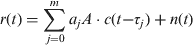
where A is the amplitude of the direct signal; a j is the amplitude of the repeater jamming signal. a 0 is the amplitude of the direct signal, a 0=1; j is the index of the repeater jamming signal; τ j is the delay of the repeater jamming signal; τ 0 is the amplitude of the direct signal and τ 0=0; c(·) is for the C/A code; and n(t) is the white Gaussian noise (i.e. with a zero mean);
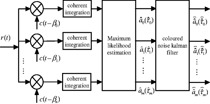
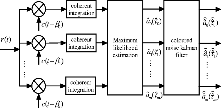
As shown in Figure 1, the process of the coherent integration of r(t) is:
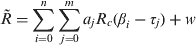
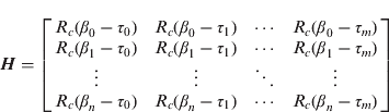
where R c(·) is the autocorrelation function of the C/A code; β i is the i-th delay estimation of the repeater jamming signal; i is the index of the estimates signal; n is the number of code delays generated in the localization; m is the number of repeater jamming signals;  is the observation matrix; and w is the noise in the coherent integration. Equation (2) can be expressed in the form of the following matrix:

where
The model for the estimation of repeater jamming.
After the coherent integration, the noise is similar with the low-pass Gaussian processes and its output can be expressed as (Gadallah, Reference Gadallah1998):

where h lpf(t) is the pulse response of the coherent integration and * denotes convolution.
The cross-correlation between w l (t) and w j (t) is:
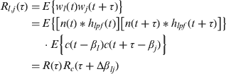
Where,

When τ=0, from equations (5) and (6), we have

Let P w=R c(Δβt ij), and let the noise covariance matrix of w=[w 0, w 1, … , w n]T be C w, then

The MLE for the amplitude scales of the repeater jamming signals can be obtained (Gadallah, Reference Gadallah1998):

Assuming R f is the mean of  and it is considered as the measurement vector in the noise-free case; let
 , then
 . Let
 denote the MLE of
 in the noise-free case and let v be its uncertainty, then
 , and can be expressed as:

3. THE MODEL FOR THE OBSERVATION NOISE IN THE KALMAN FILTER
In Figure 1, the input of the Kalman filter is the output of the MLE. A Kalman filter is usually made up of both state equations and observation equations. Based on equation (10), the observation equation at the k-th epoch can be expressed as:

The Kalman filter is an algorithm for recursively estimating the dynamical underlying state of the vectors. Therefore the time is a very important function issue in this application, which includes the jamming signal parameters and additive white Gaussian noise as a function of time according to the effects of both Doppler shift and the receiver motion. In this paper, the system dynamic can be expressed by the change in the state vector  with respect to time k. Then the state equation of the Kalman filter from the epoch k−1 to epoch k can be expressed as:

where Φk,k−1 is the state transition matrix, mostly Φk,k−1 is a diagonal matrix with its element representing the rate of change of the channel. The channel is characterised by the differences in the carrier Doppler frequencies of the jamming signal and direct signals (Gadallah, Reference Gadallah1998). In (VanNee, Reference Van Nee1992), a rough estimate for the maximum Doppler difference for the C/A-code was given as 0·62 Hz. In this section, we assume that the state transition matrix is an identity matrix (i.e. no dynamics are assumed). Then we concentrate on the study of the Kalman filter when it approaches the steady state. Once the improvement by the Kalman filter is investigated at the steady state, a comparison will be made between the steady state time versus the time of maximum Doppler difference. Let the notation nk be the noise added to the system, we assume this noise to be zero because there is no clue which shows that is corrupted with additional noise.
The state equation and observation equation of the Kalman filter become:


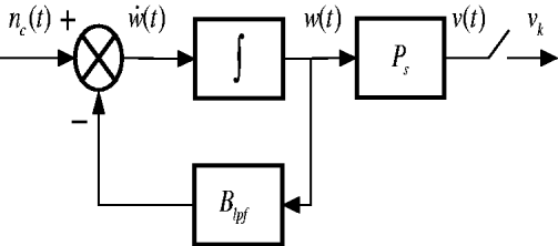
Equations (13) and (14) are the state equation and measurement equation of the Kalman filter system with coloured noise. The shaping process for the coloured noise vk is shown in Figure 2 (Gadallah, Reference Gadallah1998).
The model of the shaping filter for the coloured noise.
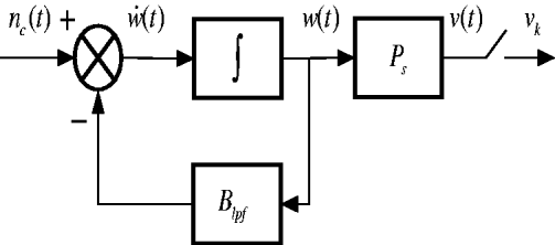
In Figure 2, w(t) is the white Gaussian noise and  is its derivative, which can be obtained by:

Where n c(t) is the zero mean white Gaussian noise. The shaping filter is for the introduction of the correlated measurement noise in the Kalman filter. The noise process can be considered as the first-order Markov process driven by white Gaussian noise. B lpf is the equivalent shaping filter bandwidth.
Multiplying equation (15) by  and then integrating it from t i to t i+1, one can obtain:

Where n dc (t i) is the noise after the integral with the mean and covariance (Tang et al., 2006):


In order to obtain v(t i), equation (16) is multiplied by P s:

Where the mean and covariance of ς(t i) are:


Equation (19) can be also expressed as:

For the discrete-time form.
In equation (22),  , Δt=t i+1−t i
Equation (22) is the expression of the coloured noise vk in the observation equation of the Kalman filter.
4. RECURSIVE FORMULAE FOR THE KALMAN FILTER WITH COLOURED NOISE
For the solution of a Kalman filter with coloured observation noise, the commonly used method is expanding the dimension of the state vector by adding extra parameters to be estimated for the noise, i.e. the coloured noise vk is treated as part of the expanded state vector. Thus the calculation burden will be increased. In this paper, the technique of differencing two consecutive epochs' observables was used. By the current epoch's (k-th) observable subtracting the ((k-1)-th) observable multiplied by Dk,k−1, the new observation will be used as a substitute for the aforementioned observation equation in the Kalman filter.
Substitute equation (22) into equation (14) to get:

Subtract the (k-1)-th epoch's observable multiplied by Dk,k−1 from the k-th observable, then:
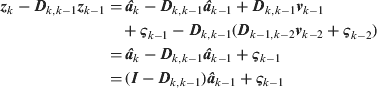
Let zdk=zk−Dk,k−1zk−1, H k=I−Dk,k−1, then the new observation equation is:

In the new observation equation, the observation noise ς k−1 is a zero mean white noise.
From the new equations for the coloured noise Kalman filter, the algorithm is summarised below.
The covariance matrix of the predicted state vector:

The Kalman gain matrix K k is:

Where Rd is the covariance of ς (t i), as shown in equation (21).
The updated covariance matrix of the estimated state vector Pk is:

The update equation for the estimated state vector is:

The initial conditions (i.e. at the initial epoch t 0 and its measurement  ) are:

5. EXPERIMENTS AND VALIDATION
5.1. Estimating repeater jamming signals based on MLE
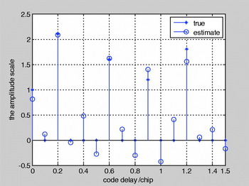
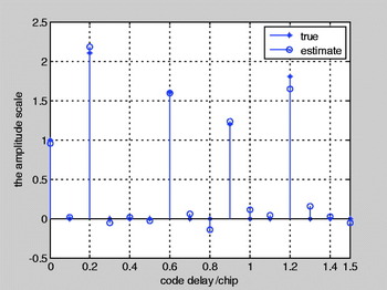
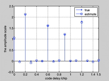
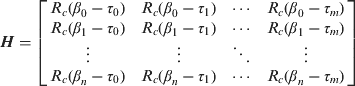
In the GPS signal simulator proposed in (Tang et al., 2006), the intermediate frequency (IF) of the signal is zero, and no noise is added. The amplitude scales of the direct signal and the repeater jamming signals are a=(1, 2·1, 1·6, 1·2, 1·8). The code phase delay of the direct signal and the repeater jamming signals are 0, 0·2, 0·6, 0·9 and 1·2 respectively. When estimating the repeater jamming signals, the search range for the code phase delay was set to β∊[0, 1·5] and the search step was set to 0·1 chip (the code phase delay will not influence the code track loop when the code delay is beyond 1·5 chip). The elements of the coefficient matrix H in equation (3) can be calculated from the correlation function:
From equation (6), the noise covariance of the low-pass filter is σ 2, so the signal-to-noise (SNR) ratio can be obtained by:

Where, T is the cumulative time of the coherent integral, A is the same as that of equation (1) and C/N 0 is the carrier-to-noise density ratio. The noise w, covariance C w, new observation matrix , P w and H can be obtained from equations (8), (2), (7) and (3) respectively. Finally, the amplitude and code delay of the repeater jamming signal can be estimated using equation (9). The results of the estimated amplitude scales based on MLE are shown in Figures 3 and 4 where the true values are the values designed in the GPS signal simulator. From these figures, it can be seen that the estimation results are influenced by the noise even in the case where the C/N 0 value is as high as 40 dB-Hz. MLE cannot estimate repeater jamming signals correctly until the cumulative time of the coherent integral reaches 20 ms.
C/N 0=40 dB-Hz, T=1 ms, MLE.

C/N 0=40 dB-Hz, T=20 ms, MLE.

5.2. Estimating repeater jamming signals based on the Kalman filter with coloured noise
The repeater jamming parameters in the GPS signal simulator for this experiment were set the same as that in experiment (1), as shown in Figure 1. The two steps of the estimation are as follows.
First, the covariance R d of the white noise ς k−1 was obtained from equation (21), where

The observation matrix Hk in the new observation equation (24) can be obtained by:

Where Δt was set to the same value as T.
Secondly, Hk, Rd and P0 (P0 is for the initial conditions) were applied to equation (27) so the Kalman gain matrix K k was calculated. Finally, using equations (26)–(29), the recursive formulae of the Kalman filter, the amplitude and code delay of the repeater jamming signal were obtained. The estimation results are shown in Figures 5 and 6.
C/N 0=40 dB-Hz, T=1 ms, Kalman filter, 1000 times iteration.

C/N 0=20 dB-Hz, T=20 ms, Kalman filter, 5000 times iteration.

Figure 5 shows that when 40 dB-Hz and 1 ms are used for the C/N 0 and the cumulative time of the coherent integral respectively, the estimates of the repeater jamming signal are comparatively accurate after 1000 iterations. Figure 6 shows that when 20 dB-Hz is used for C/N 0 and 20 ms for the time of the coherent integral, the estimates of the repeater jamming signals are accurate after 5000 iterations.
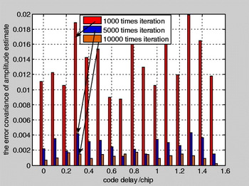
The relation between iteration time and the estimate's precision is shown in Figure 7. From this figure, it can be seen that the precision of the estimate can be improved by increasing the iteration number of the Kalman filter. An increase in the iteration time may however result in a time-consuming calculation. According to the experiment, if both computing speed and estimate's precision are taken into account, 5000 iterations are appropriate.
Relation between the iteration time and estimate's precision.

6. CONCLUSIONS
In this paper, a new method using maximum likelihood estimation and Kalman filtering with coloured noise for the estimation of repeater jamming signals was proposed. This new method is based upon the conventional multipath estimation approach. The performance of the new method was assessed. Test results show that the new method performs better than MLE, and using this method, repeater jamming signals can be precisely estimated even for the cases where the SNR is as low as 20 dB-Hz. Currently, this method has been applied in a GPS software receiver for anti-jamming experiments.
ACKNOWLEDGEMENT
Funding from the 863 Plan of China (2008AA12Z307).