1. Introduction
Self-propelling particles have drawn substantial attention recently for their myriad potential applications, such as nutrient transport (Magar & Pedley Reference Magar and Pedley2005; Michelin & Lauga Reference Michelin and Lauga2013), fertilisation processes (Medina-Sánchez et al. Reference Medina-Sánchez, Schwarz, Meyer, Hebenstreit and Schmidt2016; Magdanz et al. Reference Magdanz, Medina-Sánchez, Schwarz, Xu, Elgeti and Schmidt2017), microbial proliferation (Delarue et al. Reference Delarue, Hartung, Schreck, Gniewek, Hu, Herminghaus and Hallatschek2016) and targeted drug delivery (Nelson et al. Reference Nelson, Kaliakatsos and Abbott2010). Different self-propelling particles employ different motility mechanisms to swim in a fluid, e.g. Escherichia coli uses a run-and-tumble mechanism to propel in a fluid (Larsen et al. Reference Larsen, Reader, Kort, Tso and Adler1974); a sperm cell moves with the flagella attached to its body (Friedrich & Jülicher Reference Friedrich and Jülicher2007); Paramecium or Opalina swims by generating intricate wave patterns (called metachronal waves) on its surface (Machemer Reference Machemer1972). To understand the propulsion mechanism of these self-propelling particles, substantial research has been conducted based on various self-propelling microswimming models (Nasouri & Golestanian Reference Nasouri and Golestanian2020; Poehnl & Uspal Reference Poehnl and Uspal2021; Fung et al. Reference Fung, Bearon and Hwang2022; Lin et al. Reference Lin, Yu, Li and Gao2022; Poddar Reference Poddar2023).
Classical self-propelling models usually assume swimming linearly, focusing solely on the translational motion of the body. Consequently, the locomotion direction of swimmers is primarily affected by external flows or hydrodynamic interactions with other swimmers or obstacles. However, many microorganisms can change their swimming direction by rotating their orientational vector, causing a helical motion (Crenshaw Reference Crenshaw1993; Lee et al. Reference Lee, Brooks, Shelton, Bishop and Bharti2019; Cortese & Wan Reference Cortese and Wan2021). This motion has given rise to what is known as the ‘chiral swimmer’. Similarly, the chiral movement of artificial swimmers usually stems from any asymmetry caused by colloidal shape or defects in their catalytic coating or flagella (Ebbens & Gregory Reference Ebbens and Gregory2018; Lancia et al. Reference Lancia, Yamamoto, Ryabchun, Yamaguchi, Sano and Katsonis2019). Theoretical efforts concerning active chiral particles predominantly revolve around active Brownian particle dynamics, which effectively consider excluded volume effects but typically neglect hydrodynamic interactions of particles (Liao & Klapp Reference Liao and Klapp2018; Levis & Liebchen Reference Levis and Liebchen2018; Levis & Liebchen Reference Levis and Liebchen2019; Bickmann et al. Reference Bickmann, Bröker, Jeggle and Wittkowski2022).
To establish a chiral microswimmer while considering hydrodynamics, an alternative approach could involve utilising a modified ‘squirmer’ model. This mathematical microswimmer model, first proposed by Lighthill (Reference Lighthill1952) and later extended by Blake (Reference Blake1971b
), simulates the coordinated motion of a dense array of cilia on the surface of a microswimmer (e.g. Opalina and Volvox) through a given slip velocity distribution around its boundary. It has been successful in reproducing the flow field generated by Volvox swimming (Pedley et al. Reference Pedley, Brumley and Goldstein2016) and has found application in many microswimming scenarios, including the nutrient uptake of self-propelled organisms (Magar Reference Magar2003; Magar & Pedley Reference Magar and Pedley2005), their swimming efficiency analysis (Michelin & Lauga Reference Michelin and Lauga2010, Reference Michelin and Lauga2013), hydrodynamic interactions with obstacles (Ishimoto & Gaffney Reference Ishimoto and Gaffney2013; Ouyang et al. Reference Ouyang, Lin and Ku2018, Reference Ouyang, Lin, Yu, Lin and Phan-Thien2022), cargo-carrying problems (Thiffeault & Childress Reference Thiffeault and Childress2010) and collective swimming (Ishikawa & Pedley Reference Ishikawa and Pedley2008; Ishikawa et al. Reference Ishikawa, Locsei and Pedley2008; Zöttl & Stark Reference Zöttl and Stark2014; Lin & Gao Reference Lin and Gao2019). Recent studies have further advanced this model by incorporating chirality. Fadda et al. (Reference Fadda, Molina and Yamamoto2020) developed a chiral squirmer and considered its dynamics when sedimenting on a flat plate. This chirality was achieved by introducing azimuthal slip velocity terms exerting on the boundary of a particle for self-propelling, which are generally ignored for a classical squirmer. They find that the introduction of chirality to squirmers modifies their swimming motion, adding a third direction of motion. Burada et al. (Reference Burada, Maity and Jülicher2022) investigated the combined behaviour of two chiral squirmers, uncovering their hydrodynamic interactions that lead to attraction, repulsion and even bounded states where swimmers continue to orbit around a common average trajectory periodically. Subsequently, Maity & Burada (Reference Maity and Burada2022a
) studied both near- and far-field interactions between two chiral squirmers, observing that lubrication effects between them can convert both of their monotonic and convergence states into divergence states. Released in a flow field with chemical gradients, a chiral squirmer steers either towards or away from the source of the chemical gradient, depending on the strengths of translational velocity (
 $U$
) and rotational velocity (
 $\boldsymbol {\varOmega }$
) and the corresponding angle (
 $\chi$
) between them (Maity & Burada Reference Maity and Burada2022b
). For two chiral squirmers, the chemical gradient favours the attraction between them, sometimes resulting in a bounded state where they move synchronously (Maity & Burada Reference Maity and Burada2023). Samatas & Lintuvuori (Reference Samatas and Lintuvuori2023) further studied synchronisation in bulk suspensions of chiral spherical squirmers, revealing that a synchronised state entails velocity alignment with high orientational order in both polar and azimuthal directions. These endeavours underscore the potential of chiral squirmers in simulating natural microorganism motion. Nevertheless, the physical mechanism behind the azimuthal term (slip velocity) for chirality remains incompletely intuitive.
In present study, it is experimentally found that one defective flagellum leads to the rotation of Chlamydomonas reinhardtii in a quasi-two-dimensional plane, which hinders the diffusion process of Chlamydomonas reinhardtii. Otherwise, we adopt a numerical format that integrates our experimental findings regarding the two-dimensional rotation of Chlamydomonas reinhardtii with the classical squirmer model. This study presents experimental observations of unique behaviours exhibited by individual Chlamydomonas reinhardtii microalgae within a microcontainer. Building upon these experimental findings, numerical simulation techniques are employed to replicate these emergent phenomena. The objective is to elucidate the hydrodynamic mechanisms governing microswimmer behaviours and examine how these behaviours are influenced by external factors and the microswimmers themselves.
2. Experiments with Chlamydomonas: recurring rotation in quasi-two-dimensional space
2.1. Materials and methods
Herein, we selected Chlamydomonas reinhardtii (FACHB-265, from Freshwater Algae Culture Collection at the Institute of Hydrobiology, National Aquatic Biological Resource Center) as a model microorganism. The cells were cultivated in a sterile Tris-acetate-phosphate (TAP) medium in a dark box measuring 40
 $\rm cm$
 $\times$
40
 $\rm cm$
 $\times$
40
 $\rm cm$
, with light intensity of light-emitting diode of 40
 $\rm W$
during the daytime and 0
 $\rm W$
at night for
 $7{-}14$
days. Before experimentation, energetic cells were chosen: 15
 $\textrm {ml}$
of cell suspension was centrifuged for 10
 $\rm {min}$
at 100
 $\textit {g}$
force, leaving 3
 $\rm {ml}$
of cell suspension at the bottom of the centrifuge tube. A standing time of 60
 $\rm {min}$
was required for cell motility recovery. The cells used in this study exhibited an average length scale (major axis) of
 $d=19.4$
μm, an aspect ratio of
 $\kappa =1.27$
and a velocity of
 $U=3.92\times 10^{-5}$
 ${\rm m\, s^{-1}}$
. These physical parameters were determined through measurements conducted on a representative sample of cells, ensuring an adequate sample size for statistical significance. The background fluid medium (TAP) possessed a density of
 $\rho =1.026 \times 10^6$
 ${\rm g\, m^{-3}}$
and dynamic viscosity of
 $\mu =0.92$
 ${\rm g\, (m\,s)^{-1}}$
, as measured using an Anton Paar MCR302 rheometer. Thus, the Reynolds number of a swimming cell was estimated as
 $Re=\rho Ud/\mu \sim 0.001$
.
Herein, as shown in figure 1, a circular microcontainer, with a height of
 $h=20$
μm and a radius of
 $r_c=150$
μm, was utilised. This microcontainer was fabricated from polydimethylsiloxane (PDMS) using a standard soft lithographic technique. It comprises a cylindrical groove in PDMS, with its top surface sealed using a glass slide after being filled with a droplet of cell suspension. To increase the likelihood of capturing individual cell movement within the microcontainer, we employed two strategies. (i) Nine uniformly distributed microcontainers were simultaneously created on the feature surface of a single PDMS device (10
 $\rm mm$
 $\times$
10
 $\rm mm$
). Consequently, one droplet of cell suspension could be shared by nine microcontainers in a single experiment, thereby enhancing the probability of meeting our experimental conditions for each microcontainer. (ii) The cell suspension was diluted with TAP prior to observation. Cell movement was recorded using an inverted microscope (Nikon, Eclipse Ti) equipped with a
 $ \times 20$
or
 $ \times 40$
Nikon phase objective, a high-speed camera (Nikon, DS-Qi1Mc, 1280
 $\times$
1024 resolution, capturing at 1
 ${\rm s}$
/17 frames) and microscopic image analysis software (Nikon, NIS-Elements D 4.20.03 64-bit). To mitigate the phototactic response of cells, the microscope was situated within a dark box fitted with a bandpass interference filter (
 $\lambda =671\pm 2$
 $\rm nm$
, with a full width at half-maximum of
 $10 \pm 5$
 $\rm nm$
).
A schematic of the experiment.

2.2. Experimental results
As shown in figure 2(a), the trajectories of a single cell intuitively show a generally uniform distribution in the microcontainer, indicating a very weak wall-constraint effect. This pattern differs from the strong restriction-induced near-wall swimming observed for a single Chlamydomonas reinhardtii, as reported by Ostapenko et al. (Reference Ostapenko, Schwarzendahl, Böddeker, Kreis, Cammann, Mazza and Bäumchen2018). To elucidate this discrepancy, the details of a position are taken from figure 2(a) with figure 2(c–h) being the corresponding snapshots under the microscope. Accordingly, a profound observation in our experiment is the recurring rotation of Chlamydomonas reinhardtii near the bottom wall of the microcontainer. This near-wall rotational behaviour may account for the uniform trajectories compared with previous results. Notably, distinct highlight points are observed, particularly near the boundaries of the container, suggesting the occurrence of rotational behaviours in those regions (see the supplementary movies 1 and 2).
Trajectories (a,b,j) and relative probability density (heat maps) (i,k) of a single Chlamydomonas reinhardtii: (a,i) experimental results; (j,k) simulation results (Re = 0.01). (b) Partially enlarged detail of the trajectories highlighted by the blue square in (a). (c–h) Snapshots of the rotational Chlamydomonas reinhardtii, corresponding to the circle trajectory (marked by a green line) in (b). Plotting scale: 3.18 px μm−1 (
 $\times 20$
).

Snapshots of the rotational Chlamydomonas reinhardtii with one defective flagellum. Potting scale: 13.79 px μm−1 (
 $\times 40$
).

One might question the mechanism behind this rotation. We further observe the flagella of Chlamydomonas reinhardtii by using an inverted microscope with a
 $\times 40$
objective lens. It is found that, at the interface of fluid and solid surfaces (the boundaries of the container), an enveloped liquid film (the yellow circle) is induced, leading to the cell and one of its flagella both being captured by the fluid film (in figure 3). The defective flagellum keeps oscillating but the confinement of the liquid film leads to the characteristics of deactivation on the macrolevel. To recover normal swimming, the cell tries to escape from the confinement of the liquid film by the acute paddling of the other free flagella, leading to a rotational torque (analysed in detail in § 3). Accordingly, the Chlamydomonas reinhardtii shows rotation in a quasi-two-dimensional plane. Building upon these observations, we numerically adapt the two-dimensional squirmer model to replicating the quasi-two-dimensional rotational motion observed in our experiments. This is thoroughly discussed in § 3.
Otherwise, Chlamydomonas reinhardtii exhibits ballistic behaviour. Therefore, we further analyse mean-squared displacements (MSDs) of the cell in this experiment, as depicted in figure 4. In this section, we mainly focus on the experimental results (the black curve) and its fitting line (the red dot-dash line); other lines are analysed in § 3. On extended time scales (
 $t\gt 10$
s), the MSD reaches a plateau, consistent with the available experimental results for a single Chlamydomonas reinhardtii swimming in a quasi-two-dimensional circular domain (Ostapenko et al. Reference Ostapenko, Schwarzendahl, Böddeker, Kreis, Cammann, Mazza and Bäumchen2018). Note that our single-cell experiment is repeated more than 10 times using different cells each time. On short time scales (
 $t\leq 10$
s), the cell exhibits superdiffusive diffusion
 $\left \langle {\triangle r^2(t)} \right \rangle \sim t^{1.7}$
. This power exponent of 1.7 is smaller than that of 2.0, as reported by Ostapenko et al. (Reference Ostapenko, Schwarzendahl, Böddeker, Kreis, Cammann, Mazza and Bäumchen2018). This also is attributed to the recutting rotational behaviour of the cell (as shown in figure 2), as rotation weakens diffusion by reducing its linear travel paths.
Comparison of experimental and simulation results of the MSDs for Chlamydomonas reinhardtii (
 $t^{1.7}$
is the linear fitting result of the experimental results).

The heat maps for the motion of the cell are further collapsed into radial probability densities,
 $P(r)$
, as depicted in figure 5. We define
 $P(r)$
as follows:
 \begin{equation} P(r)= \dfrac {h(r)/(2\pi r \triangle r)}{{\int _{0}^{r_c}{\dfrac {h(r)}{2\pi r \triangle r} }{\rm d}r}}, \end{equation}
where
 $r$
is the distance from the centre of the microcontainer and
 $h(r)$
is the count of all the positions of the cell in a circular shell at distance
 $r$
with thickness
 $\triangle r$
. In contrast to the intuitive observation depicted in figure 2(a),
 $P(r)$
starts with a plateau near the centre of the container and notably increases close to the wall, consistent with the results of Ostapenko et al. (Reference Ostapenko, Schwarzendahl, Böddeker, Kreis, Cammann, Mazza and Bäumchen2018). This suggests that the rotation near the boundaries may be the cause of the contradiction between the intuitive observation and
 $P(r)$
, as depicted in figure 2(i).
Comparison of experimental and simulation results of the radial probability densities
 $P(r)$
for the cell within the microcontainer, derived from more than 10 independent experiments.

3. Partial suppression of slip velocity
3.1. Squirmer with one defective flagellum
The two-dimensional squirmer model, as proposed by Blake (Reference Blake1971a ), has been adopted to simulate the locomotion of microorganisms. This model defines a slip velocity at the surface of microorganisms through an infinite series expansion of the radial and polar components:
 \begin{equation} \boldsymbol {u}^s(r)=\sum _{n=0}^{\infty }A_n\cos (n\theta )\hat {\boldsymbol {r}}+\sum _{n=1}^{\infty }B_n\sin (n \theta )\hat {\boldsymbol {\theta }}, \end{equation}
where
 $\hat {\boldsymbol {r}}$
and
 $\hat {\boldsymbol {\theta }}$
refer to the radial and polar unit vectors for a given point on the surface of a squirmer, respectively, as shown in figure 6(d). Parameters
 $A_n$
and
 $B_n$
are the corresponding time-dependent amplitudes. For simplicity, the radial component can be disregarded (Blake Reference Blake1971a
,
Reference Blakeb
) and this simplified squirmer model is represented by the second-order truncated tangential velocity:
 \begin{equation} \boldsymbol {u}^s(\theta )=(B_1\sin \theta +2B_2\sin \theta \cos \theta )\hat {\boldsymbol {\theta }}, \end{equation}
where the coefficient
 $B_1$
contributes to the propulsion of the squirmer, determining the steady-state swimming velocity
 $U_s = B_1/2$
under Stokes flow conditions. By contrast, the coefficient
 $B_2$
determines the intensity of vorticity around the squirmer. Accordingly, a swimming parameter defined using
 $\beta = B_2/B_1$
is usually introduced to categorise squirmers into three types: pushers (
 $\beta \lt 0$
), pullers (
 $\beta \gt 0$
) and neutral squirmers (
 $\beta = 0$
). As indicated by their names, pushers (e.g. bacteria such as
 $\textit {E. coli}$
and
 $\textit {B. subtilis}$
) propel themselves from their rear ends, while pullers (e.g. algae such as Chlamydomonas reinhardtii) generate thrust from their front ends (Koch & Subramanian Reference Koch and Subramanian2011). Neutral squirmers (e.g.
 $\textit {Volvox}$
) exhibit symmetric flow without vorticity (Fadda et al. Reference Fadda, Molina and Yamamoto2020).
As previously discussed, the rotational behaviour of
 $\textit {Chlamydomonas reinhardtii}$
is hypothesised to result from one defective flagellum of the cell. Consequently, we numerically adapt the classic squirmer model by partially inhibiting the slip velocity on the boundaries of the squirmer for demonstrating the motion of a single microalga with one defective flagellum, as illustrated in (3.3) (also see figure 6):
 \begin{equation} \left \{ \begin{array}{ll} u^s\left (\theta \right ) = \left (B_1\sin \theta +2B_2\:\sin \theta \cos \theta \right )\hat {\boldsymbol {\theta }}, & \theta \in [\alpha_1^T,\alpha_2^T]\cup \in [\alpha_2^T, \alpha_1^T]\\ u^s\left (\theta \right ) = 0, & otherwise \end{array}, \right. \end{equation}
where the slip velocity operates within a specific angle range of
 $[\alpha _1^T,\alpha _2^T]$
, while being inhibited in other angle ranges. Considering the contingency of one defective flagellum, the ranges of
 $\alpha _1^T$
and
 $\alpha _2^T$
both follow a uniform distribution, i.e.
 $\alpha _1^T\sim U(0,2\pi )$
,
 $\alpha _2^T\sim U(0,2\pi )$
, at each given periodic time
 $T$
. Angle
 $\alpha =|\alpha _2^T-\alpha _1^T|$
correspondingly follows a triangular distribution, its probability density function being
 \begin{equation} p\left (\alpha \right ) =\left \{ \begin{array}{*{2}{ll}} (2\pi-\alpha)/2\pi^2, &\alpha \in [0,2\pi]\\ 0, &\textit {otherwise} \end{array}. \right. \end{equation}
Time T is defined to be negatively correlated with the translational velocity of the squirmer. According to the simulation tests, the choice of
 $T$
follows the relationship
 $T\sim 10^3/Re$
. Notably, the condition of one defective flagellum fails with
 $\alpha =2\pi$
, where this model degenerates into the classical squirmer. Lauga et al. (Reference Lauga, DiLuzio, Whitesides and Stone2006) investigated the hydrodynamic mechanisms of
 $\textit {Escherichia coli}$
swimming in circles near walls. They demonstrated that the positive rotation of the cell body generates a net viscous force on the body, while the negative rotation of its helical bundle results in a net negative viscous force on the flagella, leading to a negative torque. This torque is counterbalanced by a positive torque arising from viscous resistance to rotation. In our study, a single microalga with one defective flagellum is both force-free and torque-free, as shown in figure 6. The defective flagellum causes changes in thrust and drag (see figure 6
a,c), which are equal in magnitude but opposite in direction during steady swimming along the trajectory (force-free). However, because these forces are not collinear, they produce rotational torque. This negative torque induced by thrust and drag is counterbalanced by a positive torque resulting from the hydrodynamics of the rotation, resulting in a torque-free condition.
Schematic of mapping between (b) Chlamydomonas reinhardtii cell and (d) squirmer with one defective flagellum. A single flagellum of the cell is defective by the effect of the container boundaries, leading to the ‘thrust’ and ‘drag’ change from (a) linear to (c) nonlinear and resulting in the circular trajectory.

Herein, the motion of a single microalga with one defective flagellum is numerically simulated within a lattice Boltzmann method (LBM) framework. Further details of the method can be found in Appendix A.
3.2. Model validation
To validate the feasibility of numerically adapting the squirmer model to a squirmer with one defective flagellum, simulated results are compared with the experimental findings (as shown in figure 4). Following the experimental set-up outlined in § 2.1, within the LBM framework, the squirmer with a diameter of
 $d$
is confined within a quasi-two-dimensional circular domain (
 $d_c=15.5d$
). The squirmer is initially released at a random location within the domain, and its trajectories are tracked. As shown in figure 2, utilising dimensional conversion, the superdiffusive diffusion of the squirmer with one defective flagellum at short times (
 $t\leq 10\, \rm s$
;
 $Re=0.001$
) aligns closely with the experimental results (
 $Re \approx 0.001$
). Notably, the swimming Reynolds number for the squirmer is defined as
 $Re=\rho U_s d/\mu$
, where
 $\mu$
denotes the fluid dynamic viscosity. Furthermore, our serial code needs over 2 months to execute a calculation for low-Reynolds-number flow (
 $Re=0.001$
) while ensuring computational convergence. However, it still does not reach the desired time range of
 $t=10^3\, \rm s$
. Considering the computational time constraints, we opted to utilise a slightly higher Reynolds number (
 $Re=0.01$
) for validation purposes. Despite the absence of overlapping scales, the diffusion coefficient aligns with the experimental findings (figure 4), indicating similar hydrodynamics between the simulated and experimental scenarios. Furthermore, figure 4 illustrates that the radial probability densities
 $P(r)$
for both the cell and the squirmer (
 $Re=0.01$
) in the microcontainer exhibit exceptional agreement. Meanwhile, the heat maps depicting the relative probability density for the squirmer closely resemble those obtained from the experiments, as illustrated in figure 2(i,k). The consistency demonstrated by these findings confirms the ability of the model to accurately predict experimental outcomes. Notably, for
 $Re=0.01$
, a lattice time of
 $T = 10^5$
is employed (equation (3.3)). Hence, we find that T is not sensitive to the results of the superdiffusive behaviours for the squirmer, with lattice time of the same order of magnitude after careful testing.
3.3. Influence of parameters on the motion of a squirmer with one defective flagellum
In this section, we simulate the motion of a single microalga with one defective flagellum in an unconfined fluid to investigate the influence of finite fluid inertia, self-propelling strength (
 $\beta$
) and active angle (
 $\alpha$
) on its swimming behaviours. To provide a thorough evaluation of the hydrodynamic behaviour of the squirmer with one defective flagellum, we presume that one flagellum of each particle remains defective for an extended duration (i.e.
 $T=\infty$
), like an Effrenium voratum that keeps on rotating with its lone longitudinal flagellum (Huang et al. Reference Huang, Hu, Yang, Liu and Zhang2021). The squirmer with a diameter of
 $d=40\triangle x$
(where
 $\triangle x$
is the lattice width) is released at the centre of a computational domain with dimensions of
 $L$
 $\times$
 $L$
 $=$
20
 $d$
 $\times$
20
 $d$
. Periodic boundary conditions are applied to all boundaries. We have carefully validated our LBM code (Appendix B). We observe that the squirmer with one defective flagellum undergoes stable circular orbit motion after transient dynamics, effectively reproducing the rotation of the cell observed in our experiment. As depicted in figure 7(a), the swimming speed of the squirmer increases with
 $\beta$
to varying degrees. This contrasts with the swimming of a classic squirmer at the Stokes flow limit (where
 $Re=0.01$
can be considered), where the speed of such a squirmer remains constant,
 $U_s = B_1/2$
, regardless of
 $\beta$
(Blake Reference Blake1971a
,
Reference Blakeb
; Chisholm et al. Reference Chisholm, Legendre, Lauga and Khair2016). This difference suggests that a substantial portion of the self-propelled kinetic energy of the squirmer with one defective flagellum is converted into rotational dynamics. Moreover, the increase of Re results in a decreasing speed for such a squirmer at small
 $\beta$
values (
 $\beta \leq 2$
). With further increases in
 $\beta$
, the squirmer swims fast at large Re values. Additionally, at identical Re values, an elevated
 $\beta$
results in a large rotational diameter, which is positively correlated with the speed, as illustrated in figure 7. To illustrate the possible mechanism, we plot the pressure and velocity distributions around the squirmer with one defective flagellum, as shown in figure 8. Around the body, the pressures are clearly not symmetrically distributed, and the combined forces cause them to rotate clockwise. For small Re values (
 $Re=0.01$
; see figure 8
a,b), the outer side of the squirmer with
 $\beta =0.5$
experiences predominantly positive pressure, which is evidently smaller than that for the squirmer with
 $\beta =5$
. This elevated pressure indicates a strong self-propelled force, subsequently resulting in a fast speed. However, it is observed that the squirmer with
 $\beta =0.5$
suffers higher pressure at its head than at the rear. This contrasts with the pressure distribution of the squirmer with
 $\beta =5$
, where the elevated pressure is observed at its rear. These two different pressure distributions may induce a greater net torque at
 $\beta =0.5$
than at
 $\beta =5$
, as the positive pressure at the rear (head) contributes to the counterclockwise (clockwise) rotation, resulting in a smaller rotational diameter at
 $\beta =0.5$
. Focusing on the streamlines around the bodies, an evident loop is observed inside the squirmer with
 $\beta =0.5$
, whereas it is outside that with
 $\beta =5$
. This indicates a smaller rotational diameter at
 $\beta =0.5$
than at
 $\beta =5$
intuitively. With an increase of Re (from
 $Re=0.01$
to 1), the pressure distribution for the squirmer with
 $\beta =0.5$
remains similar (compare figures 8
a and 8
c), but that for the squirmer with
 $\beta =5$
is distorted (compare figures 8
b and 8
d). This may be relevant to the accumulation feature of vorticity for the inertial puller (
 $\beta \gt 0$
).
Swimming speed (a) and rotating diameter (b) of squirmers with one defective flagellum in an unconfined fluid with Re from 0.01 to 1.

Pressure and streamlines around squirmers with one defective flagellum: (a)
 $Re=0.01$
,
 $\beta =0.5$
; (b)
 $Re=0.01$
,
 $\beta =5$
; (c)
 $Re=1$
,
 $\beta =0.5$
; (d)
 $Re=1$
,
 $\beta =5$
. Black arrows denote clockwise rotation, and pressure is normalised using
 $\rho U_s^2$
. In such situations,
 $\alpha =180^{\circ }$
; ‘outer side’ denotes
 $0^{\circ }\leq \alpha \leq 180^{\circ }$
and ‘inner side’ denotes
 $180^{\circ }\lt \alpha \leq 360^{\circ }$
.

We further examine the effect of active angle
 $\alpha$
on the swimming speed and rotational diameter of the squirmers with one defective flagellum, as shown in figure 9. The speed of the squirmer with
 $\beta =0.5$
increases monotonically with
 $\alpha$
, suggesting the presence of somewhat linear superposition properties in the flows distributed around the body as
 $\alpha$
is increased. Consequently, the change in rotational diameters broadly coincides with the pattern of the speed (figure 9
b). Furthermore, it is observed that the speed is only slightly faster at
 $Re=0.01$
than at
 $Re=1$
, suggesting similar flow-field structures around the squirmer (
 $\beta =0.5$
) at different Re values (figure 8
a,c). Given that
 $\beta$
is responsible for generating vorticity around the squirmer, a small
 $\beta$
value indicates that only a small amount of vorticity is induced with the increase of Re. In the case of a squirmer with
 $\beta =5$
, its speed peak is achieved at
 $\alpha =180^{\circ }$
, indicating considerably nonlinear features. Furthermore, the peak of the rotational diameter coincides with that of its speed. Generally, a high
 $\beta$
results in a fast speed of the squirmer, as depicted in figure 9(a). This differs from the behaviour of a classic squirmer (
 $\alpha =360^{\circ }$
), where a high
 $\beta$
leads to a slow puller (
 $\beta \gt 0$
) owing to the inclusion of weak fluid inertia (Wang & Ardekani Reference Wang and Ardekani2012). The mechanism may be related to the rotation, which induces a more complex fluid-structure interaction affecting the rotational swimming, especially for cases beyond the Stokes flow regime.
Swimming speed (a) and rotating diameter (b) of squirmers with one defective flagellum in an unconfined fluid with active angles
 $\alpha$
from
 $30 ^{\circ }$
to
 $300^{\circ }$
.

Power expenditure for rotational swimming as a function of (a) swimming pattern
 $\beta$
and (b) active angle
 $\alpha$
in an unconfined fluid with Re from 0.01 to 1.

A swimming squirmer with one defective flagellum injects energy into the fluid through the given tangential boundary velocity. This energy is eventually dissipated within the viscous fluid. The rate of work P is hence calculated as
 \begin{equation} P=-\int _S{\boldsymbol {n}\cdot \boldsymbol {\sigma }\cdot \boldsymbol {u}_E}\,{\rm d}S, \end{equation}
where
 $\boldsymbol {n}$
is the unit normal outward from the surface
 $S$
of the squirmer and
 $\boldsymbol {\sigma }$
,
 $\boldsymbol {U}$
and
 $\boldsymbol {u}_E$
are the stress tensor, translational velocity and boundary velocity of the squirmer, as shown in (A7), respectively. Figure 10 shows the power expenditure of the squirmer with different
 $\beta$
and
 $\alpha$
. Notably,
 $P$
is the averaged results over a period (a circle), and it is normalised using
 $B_1^2\mu d/4$
. The pattern of energy expenditure for the squirmer with
 $\beta$
is akin to that of an individual classic squirmer (Magdanz et al. Reference Magdanz, Medina-Sánchez, Schwarz, Xu, Elgeti and Schmidt2017), wherein a swimmer with a high
 $\beta$
expends additional energy. Moreover, an increase in Re contributes to an enhancement in energy expenditure, with a notable increase observed when fluid inertia cannot be neglected (from
 $Re=0.1$
to 1). Additionally, with the increase in the active angle
 $\alpha$
, as depicted in figure 10(b), the energy expenditure increases monotonically. This contrasts with the non-monotonic trends observed in swimming speed and rotational diameter (figure 9), suggesting that the self-propelled mode, rather than the swimming state, typically determines the energy consumption.
4. Conclusion
Herein, we report the experimental discovery of quasi-two-dimensional rotational motion exhibited by swimming microalgae, Chlamydomonas reinhardtii, within a microcontainer. This rotational behaviour is suggested to be induced by one defective flagellum. To elucidate the hydrodynamic mechanisms underlying this phenomenon, we numerically adapt the classic two-dimensional model. Considering one defective flagellum, we particularly inhibit the slip velocity on the microalga boundary. Subsequently, we employ a LBM to simulate the motion of a squirmer with one defective flagellum in an unconfined fluid.
We observe that the speed of the squirmer with one defective flagellum increases with
 $\beta$
to varying degrees when Re is small (
 $Re=0.01$
). It appears that the swimming speed of the squirmer with one defective flagellum deviates from the Stokes flow limit associated with a classic squirmer. This deviation can be attributed to the profound conversion of the self-propelled kinetic energy of the squirmer with one defective flagellum into rotational dynamics. Furthermore, an increase in Re leads to a decrease in speed for the squirmer at small
 $\beta$
values (
 $\beta \leq 2$
). However, with a further increase in
 $\beta$
, the squirmer swims fast at large Re values. At identical Re values, a high
 $\beta$
results in a large rotational diameter, and this diameter is positively correlated with the speed.
Considering the effect of the active angle
 $\alpha$
, we observe somewhat linear superposition properties of the flows distributed around the squirmer with one defective flagellum when increasing
 $\alpha$
at low
 $\beta$
values (
 $\beta =0.5$
). By contrast, the speed for a squirmer with
 $\beta =5$
exhibits evidently nonlinear features. Furthermore, we noticed that the speed is only slightly faster at
 $Re=0.01$
compared with
 $Re=1.0$
. This suggests that only a small amount of vorticity is induced with an increase in Re at a small
 $\beta$
. Moreover, we concluded that a high
 $\beta$
results in a fast speed of the squirmer at
 $Re=0.01$
, which differs from the behaviour of a classic squirmer. This discrepancy is attributed to the rotation inducing additional complex fluid-structure interactions affecting rotational swimming.
Additionally, we present and discuss the energy expenditures for the squirmer with one defective flagellum in an unconfined fluid. We observe that the pattern of expenditures for the squirmer with
 $\beta$
is similar to that of an individual classic squirmer, wherein a swimmer with a high
 $\beta$
expends additional energy. Furthermore, we find that increases in Re and active angle
 $\alpha$
both contribute to enhancing energy expenditure.
Supplementary movies
Supplementary movies are available at https://doi.org/10.1017/jfm.2025.307.
Acknowledgements
The authors would like to thank doctoral student Pengfei Du for helping them to coordinate experimental equipment, experimental site and other experimental resources in the context of the COVID-19 pandemic. This work is also supported by the National Natural Science Foundation of China (grant nos. 12132015, 12302333), the Zhejiang Provincial Natural Science Foundation of China (grant no. LQN25A020006) and the Ningbo International Sci-tech Cooperation Projects under ‘Innovation Yongjiang 2035’ (grant no. 2024H016).
Declaration of interests
The authors report no conflict of interest.
Data availability statement
The data that support the findings of this study are available from the corresponding author upon reasonable request.
Appendix A. Numerical method
Herein, the motion of the fluid is solved through a single-relaxation-time LBM (Qian et al. Reference Qian, D’Humières and Lallemand1992). The discrete lattice Boltzmann equations are expressed as follows:
 \begin{equation} f_i\left (\boldsymbol {x}+\boldsymbol {e}_i\triangle t, t+\triangle t\right )-f_i\left (\boldsymbol {x}, t\right )=-\frac {1}{\tau }\left [f_i\left (\boldsymbol {x}, t\right )-f_i^{(eq)}\left (\boldsymbol {x}, t\right )\right ], \end{equation}
where
 $f_i (\boldsymbol {x}, t )$
is the distribution function for microscopic velocity
 $\boldsymbol {e}_i$
and
 $f_i^{(eq)} (\boldsymbol {x}, t )$
denotes the corresponding equilibrium distribution function. Here,
 $\triangle x$
,
 $\triangle t$
and
 $\tau$
are the lattice grid size, the time step of the simulation and relaxation time related to the fluid viscosity
 $\nu$
, respectively. The fluid density
 $\rho$
and velocity
 $\boldsymbol {u}$
are determined as follows:
 \begin{equation} \rho =\sum _i{f_i},\hspace {0.5cm} \rho \boldsymbol {u}=\sum _i{f_i\boldsymbol {e}_i}. \end{equation}
The classical D2Q9 (Qian et al. Reference Qian, D’Humières and Lallemand1992) lattice model is adopted, and its discrete velocity vectors are given using the following equation:
 \begin{equation} {\boldsymbol{{e}}}_i= \left \{ \begin{array}{ll} (0,0),& \text {for} \; i=0 \\ (\pm 1,0)c,(0,\pm 1)c,& \text {for} \;i=1 \;\text {to}\; 4\\ (\pm 1,\pm 1)c,& \text {for} \; i=5 \; \text {to} \; 8, \end{array} \right . \end{equation}
where
 $c = \triangle x/\triangle t$
denotes the lattice speed. The equilibrium distribution functions can be expressed as follows:
 \begin{equation} f_i^{(eq)}\left (\boldsymbol {x},t\right )=w_i \rho \left [1+\frac {3\boldsymbol {e}_i \cdot \boldsymbol {u}}{c^2}+\frac {9\left (\boldsymbol {e}_i\cdot \boldsymbol {u}\right )^2}{2c^4}-\frac {3\boldsymbol {u}^2}{2c^2}\right ], \end{equation}
where
 $w_i$
is the weight with
 $w_0 = 4/9$
,
 $w_{1-4} = 1/9$
and
 $w_{5-8} = 1/36$
. For the D2Q9 model, the speed of sound is represented as
 $c_s=c/\sqrt {3}$
. By performing a Chapman–Enskog expansion, the macroscopic mass and momentum equations at the low-Mach-number limit can be recovered as follows:
 \begin{equation} \frac {\partial \rho }{\partial t}+\nabla \cdot \left (\rho \boldsymbol {u}\right )=0 \end{equation}
and
 \begin{equation} \frac {\partial \left (\rho \boldsymbol {u}\right )}{\partial t}+\nabla \cdot \left (\rho \boldsymbol {u}\boldsymbol {u}\right )=-\nabla p+\rho \nu \nabla ^2\boldsymbol {u}. \end{equation}
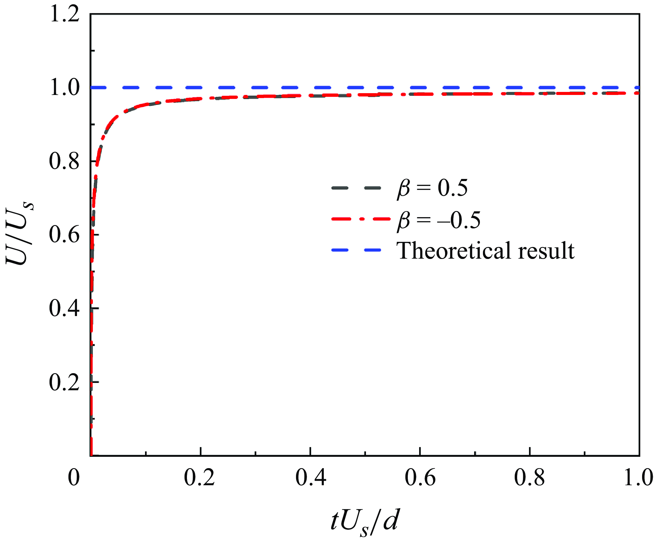
Time history of the normalised velocities (
 $U/U_s$
) of squirmers in an unconfined flow with
 $Re=0.01$
.

The kinematic viscosity of the fluid is determined using the equation
 $\nu = c_{s}^{2} (\tau -0.5 ) \triangle t$
.
To impose no-slip boundary conditions on the boundaries of the squirmer, we utilised the improved bounce-back scheme proposed by Lallemand & Luo (Reference Lallemand and Luo2003). Regarding the self-propelling dynamics, the velocity
 $\boldsymbol {u}_E$
of the boundary node is updated by adding the slip velocity, as indicated in (3.2) before the interpolations. This update can be expressed as follows:
 \begin{equation} \boldsymbol {u}_E=\boldsymbol {u}_b+\boldsymbol {u}^s=\boldsymbol {U}+\boldsymbol {\varOmega }\times \boldsymbol {R}+\boldsymbol {u}^s, \end{equation}
where
 $\boldsymbol {U}$
and
 $\boldsymbol {\varOmega }$
denote the translational and rotational speeds of the squirmer, respectively, and
 $\boldsymbol {R}$
is the position vector from the squirmer mass centre to the boundary node;
 $\boldsymbol {u}_b$
denotes the velocity of the boundary node for a passive particle. For a squirmer with one defective flagellum, the given slip velocity
 $\boldsymbol {u}^s$
is only exerted on partial boundary nodes. Additional details regarding squirmer dynamics using this boundary scheme can be found in our previous work (Nie et al. Reference Nie, Ying, Guan, Lin and Ouyang2023).
Appendix B. Validation test
To validate the accuracy of the energy-conserving LBM used in this study, we conduct simulations of a free-swimming motion of a single squirmer in an unconfined flow. It is known that in such conditions, a squirmer conforms to the Stokes flow limit: if Re is negligible, the speed of the squirmer stabilises at
 $U_s = B_1/2$
(Blake Reference Blake1971a
,
Reference Blakeb
; Chisholm et al. Reference Chisholm, Legendre, Lauga and Khair2016) over time. As shown in figure 11, when operating within Stokes flow conditions (
 $Re=0.01$
), the evolution of the speed for the squirmer closely matches the theoretical prediction.