INTRODUCTION
The traditional view of rational expectations and of rational behavior of investors explains financial time series essentially by the dynamics of fundamentals. With the additional hypothesis that information about the latter is publicly available to all market participants, this view is consistent with the single-representative-agent paradigm. Within this framework, the possibility that a share of investors have imperfect information, or a lower “degree of rationality,” is ignored on the basis that they would be driven out—via market selection—by the “smart money” investors, and/or by assuming that their impact on aggregate dynamics is negligible (Friedman, 1953; Lucas, 1978).
This somewhat naïve representation of financial markets is being increasingly questioned, from both an empirical and a theoretical point of view. From one side, a number of stylized facts—such as the volatility clustering and fat-tail distribution of assets returns—do not have a suitable explanation within this framework. Actually, much of the empirical work is handled by means of “atheoretical” models, whose aim is the statistical characterization of the stochastic process of price change.1
Examples of this approach are the GARCH family of models used to account for the heteroskedasticity of asset returns (see, e.g., Engle, 2001) and the studies put forth within econophysics to fit financial time series with stable distributions emerging in open systems (Mantegna and Stanley, 2000).
On the other hand, results from aggregation theory show that heterogeneity and nonprice interaction may dramatically change the statistical properties that characterize economic relationships between aggregate variables (Forni and Lippi, 1997; Kirman, 1992). As regards the literature on modeling of financial markets, a number of studies have pointed to the rich, and sometimes complex dynamics that can emerge from allowing for heterogeneity and interaction among investors (Brock and Hommes, 1992; Chiarella et al., 2001; Chiarella and He 2002; Lux, 1998).
A common feature of these models is that the switch between different forecasting strategies is ruled by some fitness function, in some cases accounting also for imitative effects, as in Kirman and Teyssière (2002) and in Routledge (1999). A common result is that the cost of signal extraction and information asymmetries can justify the adoption of forecasting strategies usually labeled as “psychological trading.” As Brock and Hommes (1998, 1999) put it, there can be such thing as “rational animal spirits.”
In this paper, we relax the distinction between chartists and fundamentalists to put the focus on the role of interaction among individuals during continuous trading. The aim is to investigate the dynamics emerging in a stock market, when in the investment behavior of its participants we allow for a tendency to mimic the actions of other investors, that is, to engage in herd behavior. Herding, as technical trading, is traditionally depicted as being an irrational strategy. The irrational view focuses on the psychology of investors and on their tendency to disregard their own prior beliefs and blindly follow rumors and other investors' behavior. Since the seminal works of Banerjee (1992), Bikhchandani et al. (1992), and Welch (1992), however, the possibility of “rational herding” has been recognized in various contexts: as an information diffusion mechanism; in the presence of a principal–agent problem between a manager and an investor; when the compensation structure of managers' contract has, as a benchmark, some average performance of other managers (see Bikhchandani and Sharma, 2000, for a review).
Although the measurement of the various forms of herding presents some difficulties, its empirical relevance is relatively well documented, mostly in countries where financial institutions are less developed, among fund managers in the form of momentum strategies, and more generally in contexts where information is likely not to be perfectly available to all market participants (Bikhchandani and Sharma, 2000). As regards the investigation of its effects on assets price dynamics, however—and apart from the rationale it can give for herd phenomena during bubbles and crashes, as in Avery and Zemsky (1998)—the literature is still evolving.
Some interesting studies have been put forth exploiting models borrowed from statistical physics, which provide some useful tools to deal with the problem of aggregation. To study the behavior of macrovariables, physicists do not describe the dynamic pattern of every single atom. They adopt a probabilistic approach to the analysis of the aggregate behavior, obtaining the dynamics of macrovariables such as volume and pressure from the joint probability distribution of large numbers of atoms. Since the seminal work of Föllmer (1974), this approach has been adopted to deal with aggregation also in economic modeling, where the role of atoms is played by a large number of agents.
To get a more complete, description of the dynamical effects of herding, we model the interaction among individuals by means of a mean-field effect such as in the work of Kaizoji (2000), but allowing for feedback between excess demand and actual asset price. Furthermore, in our work the external field (i.e., the natural tendency of an agent to invest or not) is endogenously determined by the asset-price fundamental solution. The structure of the model is rather simple and is meant to grasp the “raw” implications of herding for the fluctuations of asset prices. We therefore assume homogeneity between individuals, but for an idiosyncratic random term in their benefit function. In particular, we assume constant and homogeneous prior beliefs about the price that will prevail in the market (the expected price),
, which is adjusted according to the realized price sequence, P(t).
The model we obtain is a discrete-time three-dimensional dynamical system, where the three dynamic variables are the current excess demand, w(t), the current price, P(t), and the expected price at time t,
, computed using the information set available at time t−1. In each time period, the expected price adjusts to the current price according to an adaptive adjustment mechanism, the current price is updated according to an increasing function of the excess demand, and the excess demand is influenced by the difference between the current price and the expected price, according to the mean individual interaction based on the herding behavior described above.
The analysis, in the space of the parameters, of the stability properties and the main bifurcations of the three-dimensional dynamical system is facilitated by a simple change of variables that reduces the model to an equivalent unidirectionally coupled system, where the driving system is formed by a two-dimensional subsystem that gives the dynamics of w(t) and
, whereas the driven variable is the log of the expected price
.
The economic intuition behind this mathematical structure, and the related dynamical properties, can be explained using the herding behavior framework. Because of the incompleteness of the information set it is rational for the agent to consider more than the fundamental solution in order to compute the expected price. Because there is some piece of the agents' information set (the observed choices of the others) that is not used to compute the fundamental solution, agents also try to incorporate this “information subset” into their decision processes to improve the forecast of asset price movements. This nonprice interdependence between agents' decisions is characterized, in the short run, by a certain degree of strategic complementarity. As is well known from the work of Cooper and John (1988) and Brock and Durlauf (2001), this may generate multiple equilibria in the expected value of excess demand even though, as is shown in Section 2, equilibria with excess demand different from zero may not persist, because they imply price movements. Expected value dynamical inconsistency is the main source of asset price fluctuations in the model described in the following sections. In other words, multiple of equilibria in expectations are not equilibria of the market. Because they imply positive or negative expected excess demand, they will cause price movements not depending on changes in fundamentals.
This paper is organized as follows. In Section 2 we derive the dynamic model and we introduce the change of variable that reduces it to a unidirectionally coupled structure. In Section 3 we analyze the stability properties and the local bifurcations of the driving system, and we describe how the behavior of the driven variable, the expected price, can be deduced. In Section 4 some numerical simulations are given to confirm the analytical results of Section 3 and to show the strong path dependence that characterizes the market dynamics according to our model. Concluding remarks will follow in Section 5.
THE MODEL
We consider a population of investors facing a binary choice problem. The agents who decide to trade have to choose a strategy wi(t)∈{−1; +1}, where −1 stands for “willing to sell,” whereas +1 stands for “willing to buy” a unit of a given share. We do not model explicitly an optimal portfolio problem; rather the trade decisions wi(t) have to be interpreted as the marginal adjustment the agents make as they try to be advantaged by profit opportunities arising due to continuous trading information diffusion. In the following we use the following, assumptions:
- There exist two assets: a risk-free asset with a constant real return on investment r and a risky asset with price P(t) that pays a dividend, say every year, assumed to be an IID stochastic process with mean d.
- The number of agents who decide to trade the risky asset in period t, N(t), is a stationary process—with mean N—independent of agents' decisions.
- Agents observe past prices, the relative excess demand, w(t)= N(t)−1[sum ] wi(t), and the real interest rate, r, and have rational expectations about the dividend (their expected value is equal to d, the mean of the process). This means that the information set of the agent is the union of his/her private characteristics, say the set Ωi(t),2and the public information set Ω(t)={ r, d, w(t−1), w(t−2), …, P(t−1), P(t−2), …}.
The private information set will be modeled stochastically in a way that will be clear later. See equation (3).
- To make their buy/sell decision, agents evaluate an expected benefit function Vi(t), which will depend on their prior believes on the price that will prevail in the market. We assume that agents engage in rational herd behavior; that is, they expect that Vi(t) will be positively related to the other agents' buy/sell decisions.
- Price dynamics is assumed to follow the difference equation3
Essentially, the reason for a disequilibrium model comes from a previous analysis in which we implemented the rules of the Milan stock market in a simulative stock market. Simulations, using the swarm libraries developed by Pietro Terna, were able to reproduce many stylized facts in financial markets (particularly in intraday trading, even though in our analytical model there is nothing that limits the analysis to high frequencies) and we decided to get a deep understanding of the model by reimplementing it in analytical terms. Equation 1 approximates disequilibrium price movements in real stock markets, generated by the evolution of the order book.
where p(t) is the logarithm of P(t), and f(w(t)) is a deterministic term, which measures the influence of excess demand on current price variations, with properties f(0)=0, f′(w(t))>0.
- Agents have homogeneous expectations on the relative excess demand at period t, say w(t)e. Following Brock and Durlauf (2001), agents' static expectations4with respect to their information set are assumed; that is, w(t)e= w(t−1).
This hypothesis captures the idea that, in continuous trading, agents' expectation of the excess demand in every second is what they observed, in the computer terminal, a few seconds ago.

The agent's choice wi(t) is modeled as a binary random variable that describes, from the point of view of the modeler, the choice of agent i between the two strategies at time t. In other terms, the random variable wi(t) gives the probability distribution of agents' decisions conditionally on their expectations.
Because the N(t) random variables are independent, conditionally on agents' expectation, w(t)e, the average choice, will converge to the expected value due to the law of large numbers. This quantity depends, among other things, on the number of agents willing to trade. In real markets, changes in the volatility of N(t) affect the volatility of prices. The assumption of stationarity of N(t) is analytically convenient and it makes it possible to identify changes in prices that do not strictly depend on it.
Put differently, w(t) converges to its expected value, which may be computed using the law of iterated expectations:

Let us turn now to how the agents take their decision. With perfect information and perfect market efficiency, the relevant statistic to compute would be the ratio between the expected value of the fundamental solution of price dynamics, F= d/r, and the actual price, P(t), which measures the expected rate of profit (loss) when the price reaches the fundamental. Defining
as the logarithm of the expected value of the fundamental in the case of imperfect information, the relevant statistic, in logs, is
.
However, we assume that the agents do not consider the latter a sufficient statistic [assumption (iv)] to analyze the implications of herding for the assets' price dynamics. The rationale for this imitative behavior is that the agents try to extrapolate/exploit from the observed choices of the others the piece of information they are lacking.
A convenient way to model the herd component in the behavior of investors is by means of a binary choice framework with interaction (see Brock and Durlauf, 2001). Namely, we assume that the expected benefit function for the strategy wi(t) is

This equation is a standard assumption in the social interaction literature (see Brock and Durlauf, 2001). It implies that the utility, or benefit function, is affected by three additive components. The first component gives the private benefit in choosing strategy wi(t). The second is an interaction term (proportional spillovers) measuring the benefit of that choice in a situation where the expected average choice is w(t)e. Finally, the last term introduces, stochastically and from the point of view of the modeler, idiosyncratic factors and private information, Ωi(t), affecting agents' decisions.
To be precise, the first term on the right-hand is the benefit of the strategy “to buy one unit of share” (wi(t)=1) or “to sell one unit of share” [wi(t)=−1] in case the agent considered only the fundamental solution of price. The second term captures the positive spillover agent i expects from following the others' expected choices. It captures the interaction among investors, in the form of a proportional spillover Jwi(t) w(t)e. In other words, the benefit expected by agent i depends on his or her expectation about the average choice of the market, w(t)e. The positive function J(t) measures the weight given to the choices of other agents. We assume that the strength of the interaction is endogenous: when the price is far from individual expectations, the agent is less confident in the mood of the market, and gives a smaller weight to the interaction term of his/her forecast. Therefore, J(t)= J(p(t)) is a decreasing function of
with
. This assumption is made for two reasons: (1) research on herding in U.S. equity markets indicates that herding does not take place during periods of market stress or high price volatility—during periods of extreme market movements (Gleason et al., 2003; Christie and Huang, 1995); (2) to show that a sufficient level of herding may generate asset price fluctuations, which do not depend on changes in the fundamental, even when there is an adjustment mechanism in herding behavior, that is, when the herding component, in the agent's decision process, tends to disappear when the asset price goes far from the fundamental solution.5
Because it is intuitive, assuming an increasing amount of herding may easily produce asset price dynamics not related to the fundamental solution because the weight of fundamental strategies, with an asset price sufficiently far from
, eventually will becomes negligible.
The discrete choice literature calls the term
the “deterministic component of the expected benefit function.” The third term, εi(t+1, wi(t)), represents the random variables that may have different distributions under the two choices. As said previously, they capture agents' unknown (to the modeler) features. The standard assumption is that the difference between the random components is logistically distributed;6
Alternatively, one may assume that the two random components are independent and extreme-value distributed.

This probability distribution function has zero mean and variance equal to π2/(3β).
Because each agent choice is modeled as a binary random variable, with sample space {−1, 1} and a probability measure that depends on the expected average choice, these assumptions identify the probability measure of agents' choices. Stochastic decisions regarding whether to buy or to sell could be described by the probability that a given decision will yield a higher benefit than the other choice, conditional on the expectation of the aggregate choice that will prevail in period t,

Substituting equation (3) into (4) and using a logistic assumption of the error terms difference, this implies that the probability of agent- i choice, given average expected choice, is (see Leombruni et al., 2002)

We can now compute the expected value for each agent's choice:7
Equation (5) shows an important interpretation of β used in the binary choice with interaction literature. The parameter measures how quickly agents react, stochastically, to differences between the benefit functions of the two strategies. If β is 0 agents play the strategies at random. An increase of the parameter means that the agents in the market take care of the benefit function in their decision problem. In a sense they are more rational. Letting the parameter go to infinity will reproduce the deterministic decision process; that is, even a small positive difference in the benefit function of the strategy wi, compared to the other strategy − wi, will cause the agent to choose wi with probability 1.

The expected aggregate mean value of the market converges to the quantity (6), that is,8
By definition, tanh(x)=[exp(x)−exp(− x)]/exp(x)+exp(− x).

This equation defines a relation between the actual aggregate excess demand and the value expected by the agents. The expectation equilibria, then, are the points w* satisfying the equation

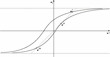
These equilibria can be represented graphically in the (w(t)e, w(t))-plane, plotting equation (7) against the 45° line, as in Figure 1. The number of equilibria will depend on the steepness of the hyperbolic tangent in the flex point, and on the value of its intercept with the w(t)-axis,
. When the current price is equal to the fundamental, the intercept is zero, and the number of equilibria will depend just on the steep of the hyperbolic tangent at the origin. In the figure, we draw an equilibrium point w′ (the rightmost curve) corresponding to a positive slack between the fundamental and the current price [
]. Suppose that the equilibrium is stable.9
An analytical discussion of stability is in Section 3.

Graphical representation, in the (w(t)e, w(t))-plane, of the equation that gives the expectation equilibria.
This equilibrium in the expectations, however, cannot be a consistent equilibrium for the market. In fact, at w′ there is a positive excess demand; this will imply a rise in the asset price, the difference
will decrease, the intercept will decrease, and the hyperbolic tangent will shift to the right. Even assuming that the equilibrium w′ will adjust smoothly to the shift in the hyperbolic tangent, this movement will stop when the curve will eventually become tangent with the 45° line (point w″). A further shift will imply no equilibrium points in the first quadrant, and the system will move toward negative excess demands, say at a point close to w‴, where an opposite movement will start.
So far, we did not consider any dynamics of the priors about the expected price. Actually, when an investor follows the herd because of the (assumed) presence of information asymmetries, he or she should coherently revise his or her priors. For instance, if he/she follows the herd during a bull market, we should expect that he or she will contextually increase his or her prior on the fundamental. More generally, we can model the priors revision by assuming that the agents adjust their private expectations, comparing them with the public information that is currently mirrored in the price level. That is, we can assume the following adaptive adjustment mechanism for the priors on the expected price,10
An adaptive rule is used for expectation formation for the sake of simplicity. This kind of rule is consistent with the assumptions in the model because changes in price are determined by changes in expected demand that, in their turn, are determined by previous expected and actual price and so on recursively. The parameter ρ captures the agent's signal extraction process.

where ρ∈[0, 1] is a measure of the adaptive speed of adjustment.11
The parameter ρ captures also the agent's signal extraction process—in other words, how much of price variation is due to fundamental variation.
.
Putting together equations (1), (7), and (8), the time evolution of the dynamic variables w(t), p(t), and
is described by a three-dimensional discrete dynamical system given by the repeated application (iteration) of the map
, defined as

where ρ∈[0, 1], β>0, f:R→R is a sign-preserving function, with f(0)=0 and f′(w)>0, J:R→R+ is a decreasing function with 0< J(0)<+ ∞. Notice that we assumed static (or naive) expectations, that is, we(t+1)= w(t) [assumption vi]. Starting from a given initial condition,

the iteration of (9) uniquely determines the trajectory

that represents the time evolution of the system. We are interested in studying the behavior of the system, how it is influenced by the parameters of the model, and the role played by the initial conditions (10). Indeed, the nonlinear three-dimensional discrete dynamical system (9) may exhibit quite different, and in some cases complicated, dynamic scenarios, and qualitative changes, or bifurcations, of the dynamic behavior can be observed as the parameters of the model are varied. Moreover, as we shall see, both the evolution of the actual price p(t) and expected
, crucially depend on the initial conditions; that is, the model (9) exhibits a strong path dependence.
To obtain a mathematically more tractable form of the dynamical system (9), we introduce the dynamic variable q(t), defined as

which represents, in each time period t, the difference between the current price and the expected price. Introducing this change of variable into (9), we obtain a dynamical system in the variables
expressed by

Of course, this model is equivalent to the model (9), in the sense that the two models are topologically conjugate, but the model in the form (13) reveals a property that simplifies its mathematical analysis: the first and second dynamic equations in (13) only involve the dynamic variables w and q; that is, they represent an autonomous two-dimensional dynamical system by the iteration of a two-dimensional map, say T2:(w(t), q(t))→(w(t+1), q(t+1)). This means that the dynamics of w(t) and q(t) are not influenced by
, whereas the time evolution of
is influenced by the dynamics of the two-dimensional system governed by T2(w, q) due to the presence of q(t) in the third dynamic equation. Following the terminology adopted in the physical and engineering literature, we can say that the expected price
is “driven by” the two-dimensional dynamic system T2: (w(t), q(t))→(w(t+1), q(t+1)), which, accordingly, is called the “driving system.” In other words, the study of the dynamic behavior of the three-dimensional model (13) is essentially reduced to the study of the two-dimensional map T2, and then the dynamics of
are deduced from it. A dynamical system characterized by this property is also denoted as unidirectionally coupled or skew-product (see, e.g., Stark, 1997).
In our case, in each time period t, the expected price
can easily be obtained from the time series { q(τ), τ=0, …, t−1} by the closed form

That is, starting from an initial12
Concerning the meaning of choosing an initial condition for the expected price, one can assume that a random perturbance occurres at t=0, so that an arbitrary initial condition can be taken. Then the dynamics are generated by iterations of equations (9), starting at those initial conditions, so that we can study the influence of such initial perturbation on the subsequent evolution of the system.
, the expected price at time t is determined by adding the algebraic sum of
observed in the past, modulated by the parameter ρ (a higher value of ρ determines a stronger influence of the past history on
, whereas ρ→0 implies no changes of the expected price, that is,
∀ t≥0). However, even if one knows the kind of behavior of q(t), the analysis of the corresponding behavior of
, given by (14), is not straightforward. First of all, a necessary condition for the convergence of
to a finite stationary asymptotic value is that q(t) goes to 0 as t increases; that is, the discrepancy between the expected and the realized price vanishes. However, even if
converges, its limiting value
is strongly influenced by the transient part of the sequence { q(t)}, determined by the driving system, before it enters a neighborhood of 0. This implies that
is highly path-dependent, because any change of the initial condition (w(0), q(0)) of the driving system causes a change of the asymptotic value
of the expected price (and consequently of the current price, because
convergent to zero). This means that any exogenous shocks or other historical accidents are “remembered” by the system; that is, their effects are not canceled by the endogenous dynamics, resulting in a long-memory property for the financial time series.
Of course, if the dynamic behavior of the driving system is such that q(t) converges to a positive steady state (or any attractor characterized by positive values of q), then
will grow indefinitely (this may be termed invest cascade13
Following Bikhchandani and Sharma, we say that an “invest (reject) cascade” occurs when individuals, acting rationally, will invest on an asset (will reject it) regardless of what their private signals tell them about the future value of the investment, because of the “domino effect” (informational cascades) typical of herd behavior (Bikhchandani and Sharma, 2000).
will decrease indefinitely (reject cascade). Instead, if the dynamics governed by the driving system exhibits bounded oscillatory behavior that involves both positive and negative asymptotic values of q(t), then more complicated and uncertain behavior will characterize the dynamics of
: when positive and negative values of q(t) balance one may get oscillatory convergence or bounded persistent oscillations of
, whereas invest (reject) cascades may be obtained if positive (negative) values of q(t) prevail in the oscillatory dynamics of the driving system.
However, in any case, the evolution of
, that is, the equilibrium value of
in the case of convergence, or of disequilibrium dynamics or of complex bounded dynamics, is strongly influenced by the initial condition (w(0), p(0)) of the driving system.
DYNAMIC PROPERTIES OF THE UNIDIRECTIONALLY COUPLED SYSTEM
In this section we study the dynamic properties of the driving two-dimensional system

that governs the time evolution of the dynamic variables w(t) and
, and how the time evolution of the expected price
is forced by the driving system, according to (14).
The steady states (or equilibria) of the two-dimensional driving system (15) are given by the fixed points of the map (15), solutions of the system T2(w, q)=(w, q), that is,

The w coordinates of the equilibria are given by the intersections between the line y= w and the sigmoid curve of the equation y=tanh [β(− f(w)/ρ+ wJ(| f(w)/ρ|)]. One realizes immediately that E0=(0, 0) is always a solution of (16), and two further solutions of (16) exist, say E+ and E−, with w>0 (hence q>0) and w<0 (hence q<0), respectively, provided that the slope at w=0 of the sigmoid curve is greater than 1; that is,

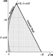
The set of parameters f′(0), J(0), β, and ρ such that the equilibrium E0=(0, 0) is locally asymptotically stable under the driving system (15) can be represented as a stability region in the plane of the parameters f′(0), J(0), shown in Figure 2, bounded by the coordinate axes, the straight line with equation

and the straight line with equation


Stability domain of the equilibrium E0=(0, 0) of the two-dimensional driving system (15).
This is stated in the following proposition, proved in the Appendix, which defines the range of parameters such that E0 is a locally asymptotically stable equilibrium of (15), and characterizes the local bifurcations through which it loses stability.
PROPOSITION 1. If the parameters satisfy the two conditions

then the fixed point E0=(0, 0) of the driving system (15) is locally asymptotically stable. Moreover, inside the parabola with equation

(the light grey region in Figure 2), the convergence occurs through damped oscillations; outside the parabola (the darker portion of the stability domain shown in Figure 2), the convergence of the driving system to E0 is nonoscillatory.
If the parameters exit the stability region of E0 through the bifurcation condition P(1)=0 with
, then the fixed point E0 of the driving system (15) undergoes a pitchfork bifurcation at which two stable equilibria E− and E+ are created, with negative and positive coordinates respectively, each with its own basin of attraction.
If the parameters exit the stability region of E0 through the bifurcation condition
with P(1)>0, then the fixed point E0 of the driving system is transformed from a stable focus into an unstable focus and stable oscillations around it characterize the dynamics of (w(t), q(t)).
From this proposition (see also Figure 2) it is easy to deduce that increasing values of β, f′(0), and J(0) may cause a loss of stability of E0 under the dynamics of the driving system (15). In particular, if J(0), which represents the interaction among agents when the expected price prevails, is too high, namely J(0)≥(1+ρ)/β, then E0 cannot be stable. The same conclusion holds if the reactivity of the current price to nonvanishing excess demand is too high, namely f′(0)>1/β. Finally, we want to stress the role of the β parameter. In the social interaction literature it measures, in a sense, agents' rationality—in other words, how quickly agents switch to better strategies (i.e., with higher values of the benefit function). Results of the stability analysis seem to be counterintuitive. The more agents are rational, in the sense above, the more unlikely the stability conditions are. But they are in line with a recent publication showing that long-term investment decisions in buying a share, vis-à-vis short-term speculative decisions, are able to stabilize the market and, furthermore, give better profits (see Liera and Beltratti, 2000).
To sum up, the analysis of the stability and local bifurcations described above reveals some different kinds of dynamics of the variables w(t) and q(t), governed by the driving system (15):
- convergence to the steady state E0=(0, 0), which convergence may be oscillatory or monotonic;
- a situation of bistability, with stable equilibria characterized by positive and negative coordinates, respectively, whose basins of attraction are separated by the stable set of the saddle point E0;
- periodic or quasi-periodic oscillations along closed invariant curves located around the unstable focus E0.
As we shall see, other kinds of dynamic scenarios can be observed, especially in the region of the parameter space characterized by β J(0)>1+ρ, that is, when we consider high levels of interaction among agents. However, we are now interested in studying the different time evolutions of the expected price
that are induced (or driven) by the different dynamic scenarios of the driving system described above.
Let us consider, first, situation (a). In this case, starting from an initial condition (10) with
belonging to the two-dimensional basin of attraction of the stable equilibrium point E0, the three-dimensional system described by (13) will converge to a steady state of coordinates
, with
, where S is the finite sum of the convergent series (14). In fact, after the initial steps, such trajectories will enter a neighborhood of E0=(0, 0), and, because E0 is a hyperbolic asymptotically stable equilibrium, both the dynamic variables w(t) and q(t) will converge to zero at an exponential rate. This means that the asymptotic portion of the series (14) behaves as a convergent geometric series. Of course, the stationary limiting value
at which the fundamental price settles [which is also the value to which the current price p(t) converges, because
tends to zero] is quite difficult to forecast, because it depends both on
and on the algebraic sum of the values of q(t) along the whole trajectory governed by the driving system (also the transient portion). In other words,
is quite strongly influenced by the initial conditions, not only by
, as explicitly expressed by (14), but also on the initial condition (w(0), q(0)) of the driving system (15). This path dependence is typical of systems with herding; see, e.g., Bikhchandani and Sharma (2000). Examples of such path dependence will be given in the next section.
Case (b) shows the typical magnetization behavior characterizing social interaction phenomena.14
The term magnetization comes from the fact that the first model, using the statistical physics framework, studied the magnetization of materials.
is quite peculiar: if the initial condition (w(0), q(0)) of the driving system (15) belongs to the basin
of the stable equilibrium with negative coordinates, then q(t) converges to a negative value. That is, the expected price is persistently lower than the realized one, and consequently a reject cascade occurs. Instead, if the initial condition of the driving system belongs to the basin
of the stable equilibrium with positive coordinates, then q(t) converges to a positive value. That is, the expected price is higher than the realized one, and consequently an invest cascade occurs.
From an economic point of view this increase in
depends on the increase in the expected market excess demand. In other terms, there is some kind of self-fulfilling prophecy at work here. Obviously, in real markets this kind of ever-increasing (-decreasing) dynamics cannot continue forever because of circuit-breaker-like mechanisms that, for the sake of simplicity, we have not included in our model.
In case (c), the motion of the driving system is characterized by self-sustained oscillations around E0, which involve both positive and negative values of w(t) and q(t). In particular, the sequence { q(t)}, which constitutes the set of terms of the series (14), is an oscillating sequence involving positive and negative values. This implies that it is very difficult, in this case, to forecast the behavior of the expected price
. It may exhibit bounded oscillations or oscillatory divergence. Indeed, as we shall see in the next section, both cases may occur, and the transition from the former to the latter situation, or vice versa, may occur as a consequence of small variations of the parameters or of the initial conditions (i.e., an exogenous shock). So we can say that for the sets of parameters that, in the driving system, give rise to stable oscillations around E0, we get more uncertain price behavior, in the sense that the kind of dynamic evolution of the price is very sensitive to parameter variations as well as to exogenous shocks that cause small changes of w and/or q.
The arguments given above can be summarized in the following proposition:
PROPOSITION 2
- If the fixed point E0=(0, 0) of the driving system (15) is stable, any trajectory of (9) starting from an initial condition with such that the point belongs to the basin of attraction of E0 converges to a steady state with where is the finite sum of the series (14). The convergence is nonoscillatory if f′(0)< fosc, whereas it occurs through damped oscillations if f′(0)> fosc.
- If two stable equilibria E− and E+ of the driving system (15) exist, with negative and positive coordinates respectively, then the trajectories of (9) starting from an initial condition with are characterized by increasing values of p(t) and (i.e., an invest cascade) if the initial condition (w(0), q(0)) of the driving system belongs to the basin of E+, but by decreasing values of p(t) and (i.e., a reject cascade) if (w(0), q(0)) belongs to the basin of E−.
- If the dynamics of (w(t), q(t)) governed by the driving system (15) are characterized by persistent oscillations around E0, then the corresponding time paths of the forced variable may show an oscillatory convergence to a bounded value, or bounded persistent oscillations, or oscillations with an increasing or a decreasing trend. The average values of the oscillating sequence as well as the increasing or decreasing trend, are strongly influenced by the initial conditions (w(0), q(0)) of the driving system (15).
We end this section by considering the case β J(0)≥1+ρ, that is, high interaction among agents. In this case, the stability conditions (20) cannot be satisfied; hence the equilibrium point E0 is unstable.
If β J(0)=1+ρ then fp= fosc= fh=ρ2/β. In this case, a simple analysis of the characteristic equation P(λ)=λ2−2λ+β f′(0)+1−ρ2=0 reveals that
- If f′(0)<ρ2/β then the eigenvalues are both real, with 0<λ1<1<λ2, so E0 is a saddle point and two further equilibria exist;
- If f′(0)=ρ2/β then λ1=λ2=1;
- If f′(0)>ρ2/β then the eigenvalues are complex conjugate and outside the unit circle; that is, E0 is an unstable focus.
If β J(0)>1+ρ then fh< fp< fosc. In this case fp and fh no longer represent bifurcation values at which the stability property of E0 changes, because E0 is always unstable. However, as f′(0) moves along these values, interesting changes in the dynamic behavior, both of the driving system (15) and of the forced variable
, can be observed. We shall illustrate these cases in the next section, through some numerical explorations.
NUMERICAL SIMULATIONS
In this section we provide some numerical simulations, in order to confirm the analytical results of Section 3 and to demonstrate the strong path dependence that characterizes the dynamic behavior of our model. In the mathematical analysis on the existence, stability, and local bifurcations of the equilibria, in the previous section, we were able to work with general functions f and J satisfying the general properties described in Section 2. Now, in order to perform the numerical simulations of the dynamical system (9), we shall use the following expressions:15
With this particular choice, the parameters used in the bifurcation analysis given above are f′(0)= k and J(0)= A. Because the parameter B does not appear in the local bifurcation results, without loss of generality we shall use a fixed value for it, namely B=2.

The first expression is a commonly used linear function of price adjustment with respect to the excess demand. This specification is compatible with the standard tâtonnement idea, because it assumes a proportionality between price changes (or return) and excess demand (see Cont and Bouchaud, 2000). The k parameter measures the sensitivity of asset price to fluctuations in excess demand. The expression of the function J proposed in (22) is just a very simple choice possessing the properties of the function J(t) described above. The parameter A is the value of the interaction at 0, J(0), whereas B measures the velocity at which the strength of the interaction decreases when the asset price move away from the expected price.
Asymptotic Stability
We start our numerical explorations by considering a set of parameters such that the equilibrium E0 of the driving system is asymptotically stable, that is, the case (a) described in Section 3, by using the set of parameters β=1.2, J(0)=1, ρ=0.6, and f′(0)=0.2. To show the property of path dependence, that is, the sensitivity with respect to the initial condition of the driving system, of the asymptotic stationary value
of the expected price, we consider two different initial conditions of the driving system (15), namely w(0)=1, q(0)=0.5 and w(0)=1, q(0)=−0.5, which generate two different trajectories of the driving system both converging to E0, represented in Figure 3a by gray squares and white circles, respectively. In Figure 3b the corresponding numerical computations of two time paths of
are shown, both starting from the same initial expected price
, but with the two different initial conditions w(0) and q(0) considered in Figure 3a. It is evident that even if both the time paths of
start from the same initial value
and both the time paths of the sequence { q(t)} converge to zero, the different transients of the trajectory { w(t), q(t)} governed by the driving system (15) lead to different equilibrium values of the expected price. Notice that in both trajectories, the equilibrium value
is reached through damped oscillations; since f′(0)> fosc, the trajectories of the driving system tend to E0 through damped oscillations that involve positive and negative values of q(t). Another aspect that is worth noticing is that our numerical explorations of the driving system (15) show that whenever the parameters are such that the equilibrium E0 is stable, it appears to be globally asymptotically stable; that is, any initial condition generates a trajectory converging to E0. So we are led to conjecture that the statement of Proposition 1 holds for any initial condition (10).

With the set of parameters β=1.2, J(0)=1, ρ=0.6,and f′(0)=0.2 the equilibrium E0 of the driving system is stable. (a) Two trajectories of the driving system generated starting frominitial conditions w(0)=1, q(0)=0.5 and w(0)=1, q(0)=−0.5, represented by gray squares and white circles, respectively. (b) The corresponding numerical computations of two time paths of $\bar{p}(t)$, both starting from the same initial expected price $\bar{p}(0)=2$, but with the two different initial conditions w(0) and q(0).
Bistability Case
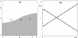
We now consider a set of parameters such that the situation of bistability described in case (b) of Section 2 holds. For example, in Figure 4a, obtained with parameters β=1.2, J(0)=1, ρ=0.6, and f′(0)=0.02< fp=0.1, the two basins
and
are represented in white and gray, respectively, separated by the stable set of the central point E0 (a saddle point). In Figure 4b two time paths of
are generated starting from the same initial expected price
, but with different initial conditions of the driving system (15), namely w(0)=1, q(0)=−0.5 belonging to
and w(0)=1, q(0)=0.5 belonging to
. As expected on the basis of Proposition 1, the former initial condition generates an invest cascade, that is, an increasing sequence
, and the latter initial condition generates a reject cascade, that is, a decreasing sequence
. Of course, because
and q(t) tends to a finite value, the same kind of time evolution of
also holds for the realized price p(t). In other words, the agents' ability to forecast the expected price seems to be offset by movements of the realized price at the same velocity, thus causing bubbles. Also, in this case, from the numerical results we try to make some inferences about the global structure of the basins of attraction, because such information cannot be deduced from the local analysis of the previous section. Looking at the simple structure of the basins
and
of Figure 4a, one may guess that when the parameters are such that a situation of bistability is present, sufficiently negative values of q(0) imply an invest cascade, and sufficiently positive initial values q(0) imply a reject cascade. However, numerical explorations of the driving system prove that the situation may be significantly different, in the sense that other sets of parameters may give more complicated structures of the basins, in particular in the presence of high levels of interaction among agents, that is, high values of J(0) (an example is shown below; see Figure 9a).

With parameters β=1.2, J(0)=1, ρ=0.6, and f′(0)=0.02 two stable equilibria of the driving system, denoted by E− and E+, coexist. (a) The basins $\mathcal{B}(E_{-}) $ and $\mathcal{B}(E_{+})$ are represented by white and gray areas respectively. (b) Two time paths of $\bar{p}(t)$ are generated starting from the same initial expected price $\bar{p}(0)=2$, but with different initial conditions of the driving system (15), given by w(0)=1, q(0)=−0.5, belonging to $\mathcal{B}(E_{+})$, and w(0)=1, q(0)=0.5, belonging to $\mathcal{B}(E_{-})$.
Neimark–Hopf Bifurcations
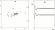
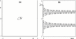
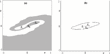
We now move to the numerical exploration of the more interesting case (c). Figure 5 is obtained with parameters β=1.2, J(0)=1, ρ=0.6, and
, just after the occurrence of the Neimark–Hopf bifurcation. In Figure 5a the phase space (w, q) of the driving system is represented, with the stable closed curve around the unstable focus E0, on which the driving system exhibits a quasi-periodic motion. Also, in this case, in Figure 5b two time paths
are shown, starting from the same initial expected price
, but with different initial conditions (w(0), q(0)) of the driving system. Even if, for any initial condition (w(0), q(0)), all the trajectories of the driving system exhibit the same long-run motion along the attracting closed invariant curve shown in Figure 5a, the behavior of the sequence
is influenced by (w(0), q(0)), as clearly shown by the two sequences represented in Figure 5b. All the different sequences
that we have numerically generated with this set of parameters and different initial conditions (w(0), q(0)) exhibit bounded oscillations.

With parameters β=1.2, J(0)=1, ρ=0.6, and f′(0)=0.44. (a) The attractor located along a closed invariant orbit around E0 is represented in the phase space (w, q) of the driving system (b) Two time paths $\{\bar{p}(t)\}$ are shown, starting from the same initial expected price $\bar{p}(0)=2$, but with different initial conditions (w(0), q(0)) of the driving system.
However, we cannot assert that the dynamics of the driving system that are characterized by bounded oscillations of (w(t), q(t)) always force bounded oscillations of the corresponding
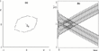
. In order to stress this point, let us consider the sequence of numerical simulations shown in Figures 6, 7, and 8. In Figure 6 we show that, with the same set of parameters β, J(0), and ρ as in Figure 5, and f′(0)=0.547, the behavior of the generic trajectory of the driving system is again characterized by bounded oscillations involving positive and negative values of the variable q(t), but the corresponding time evolutions of the expected price
exhibit oscillatory behavior with an increasing trend. Moreover, as shown in Figure 6b, even starting from the same initial fundamental price, again
, the trend may be increasing (thus leading to an invest cascade) or decreasing (thus leading to a reject cascade) according to the initial condition (w(0), q(0)) of the driving system. For example, in Figure 6b increasing prices are obtained with (w(0), q(0))=(−1, 1) and decreasing prices are obtained with (w(0), q(0))=(1, −1).

With the same set of parameters β, J(0), and ρ asin Figure 5, and f′(0)=0.547. (a) Attractor in the phase plane (w, q) of the driving system. (b) Two time evolutions of $\{\bar{p}(t)\}$ obtained starting from the same initial fundamental price, again $\bar{p}(0)=2$, and two different initial conditions,(w(0), q(0))=(−1, 1) and (w(0), q(0))=(1, −1).

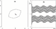
The same as Figure 6 with f′(0)=0.54.

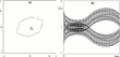
The same as Figure 6 with f′(0)=0.55.
Starting from the dynamic scenario illustrated by Figure 6, situations characterized by bounded behavior of
can be obtained by slight modifications of the parameters. For example, the situation shown in Figure 7 is obtained with the same parameters and initial conditions as in Figure 6, the only difference being a slightly smaller value of the parameter f′(0), decreased from 0.547 to 0.54. Analogously, the situation of bounded oscillation shown in Figure 8 is obtained after a slight increase of f′(0), namely f′(0)=0.55. We stress that in all the situations shown in Figures 6, 7, and 8 the asymptotic dynamics of the driving system are practically identical, and nevertheless quite different time evolutions of the fundamental prices are obtained. This confirms what we stressed at the end of Section 2 about the difficulty of forecasting the kind of long-run dynamics of prices when persistent oscillations around E0 are present in the driving system.
Such “windows” characterized by bubbles due to slight variations of one or more parameters can be numerically observed in many different parameter constellations.
Different Dynamic Scenarios
To end this section on numerical experiments, we consider some different dynamic situations that cannot be detected by the local analysis performed in Section 3. As anticipated above, some interesting dynamic scenarios can be observed when high values of J(0) are considered, that is, high levels of interaction among agents. For example, Figure 9a is obtained with the set of parameters β=1, J(0)=1.7, ρ=0.5, and f′(0)=0.18, so that β J(0)>1+ρ. With this set of parameters we have fh=0.15< fp=0.35 and fosc=0.36. Hence, f′(0)=0.18 is such that fh< f′(0)< fp. This means that the driving system has three equilibria, and the central one, E0, is unstable. For this set of parameters the two nonvanishing equilibria E− and E+ are stable foci. So the situation of bistability described at point (b) of Section 3 is obtained, and invest or reject cascades will be observed according to the choice of initial condition (w(0), q(0)) in the basin of attraction of E+ or E−, respectively. A remarkable feature that can be noticed in Figure 9a, is that in this situation the boundary that separates the basins of attraction E− and E+, represented by the white and the gray regions respectively, is more complicated than in the situations previously analyzed (see Figure 4).

(a) With parameters β=1, J(0)=1.7, ρ=0.5, and f′(0)=0.18, so that β J(0)>1+ρ, a situation of bistability is obtained for the driving system, the two non-vanishing equilibria E− and E+ being stable foci. (b) With f′(0)=0.3 the three equilibria are all unstable (E0 is a saddle point, E− and E+are unstable foci) and an attracting closed invariant curve exists that surrounds the three equilibria.
Other interesting dynamic scenarios can also be observed for greater values of f′(0), when three equilibria exist, but all are unstable. For example, in Figure 9b, obtained with the same parameters as Figure 9a except f′(0)=0.3, three equilibria exist, but they are all unstable (E0 is a saddle point, E− and E+ are unstable foci), and an attracting closed invariant curve exists that surrounds the three equilibria. Also, in this case, bounded oscillatory dynamics are observed for both the expected and the current price. We do not enter into the details of the local and global bifurcations that mark the transition from the dynamic scenario of Figure 9a to the one shown in Figure 9b. The interested reader may find descriptions of similar dynamic situations, even if in relation to different models, in some recent papers by Bischi et al. (2001) and Dieci et al. (2001).
CONCLUSIONS
We have considered the dynamic effects of herding in the buy–sell decisions of heterogeneous investors and in the consequent adjustment in individual priors about the fundamental. The incompleteness of the agents' information set is shown to be a sufficient condition for the presence of nonfundamentalist analysis in the agents' decision process modeled, in this work, on a binary choice setting with interaction.
The three-dimensional nonlinear discrete dynamical system derived from the model exhibits quite different, and in some cases complicated, dynamic behaviors. The analytical study and numerical explorations of the system allowed us to state the following results: the system may show convergence to steady state with excess demand equal to zero and asset price equal to the fundamental solution, and such convergence may be oscillatory or monotonic. Increasing the sensitivity of the risky asset price to the relative excess demand may determine a loss of stability through two possible bifurcation paths. First is a supercritical Neimark–Hopf bifurcation, at which the equilibrium of the driving system is transformed from a stable focus to an unstable one, and a stable closed invariant circle is created around it, on which the dynamics of the driving system are characterized by periodic or quasi-periodic motion. This shows the possibility of asset price movements that are not determined by changes in the asset price fundamental solution, but by agents' herd behavior. Second, the loss of stability of the equilibrium point is associated with the creation of two new equilibria via a supercritical pitchfork bifurcation: the steady state becomes unstable (a saddle point) and two stable equilibria are created, characterized by positive and negative coordinates respectively, whose basins of attraction are separated by the stable set of the saddle point, characterized by excess demand equal to zero and asset price equal to the fundamental solution. This magnetization phenomenon, typical of social interaction models, can explain real situations in which the price goes up or down so quickly that the market has to activate the circuit-breaker mechanism.
Other kinds of dynamic scenarios can be observed with sufficiently high levels of interaction among agents. However, the most striking feature of the model is that the evolution both of the price and of the expected price crucially depend on the initial conditions; that is, the model exhibits strong path dependence. This is observed in many different dynamic situations: the expected price converges to the realized price, both when the behavior is characterized by bounded oscillations (periodic and quasi-periodic trajectories), and even when the price trends up or down, depending on the initial condition, because of invest or reject cascades. This kind of path dependence seems to be strongly conditioned by the velocity at which agents forecast the expected price compared to the rapidity of asset price movements.
APPENDIX
PROOF OF PROPOSITION 1
The study of the local stability of the fixed point E0=(0, 0), under the driving dynamical system, is based on localization, on the complex plane, of the eigenvalues of the Jacobian matrix of the map (15)

computed at E0=(0, 0); that is,

The eigenvalues are the solutions of the characteristic equation P(λ)=λ2−Trλ + Det=0, where Tr=1−ρ+β J(0) and Det=β[f′(0)+(1−ρ) J(0)] are, respectively, the trace and the determinant of the Jacobian matrix computed at the fixed point E0. A sufficient condition for the stability of E0 is expressed by the system of inequalities

which give necessary and sufficient conditions for the two eigenvalues to be inside the unit circle of the complex plane (see, e.g., Gumowski and Mira, 1980, p. 159, or Medio and Lines, 2001, p. 52, or any standard book on discrete dynamical systems). Because P(−1)=β f′(0)+(2−ρ)(1+β J(0))>0 for all the values of the parameters, the stability conditions reduce to (20). The locus of points such that Tr2−4Det=0, represented by the parabola with equation (21), separates the stability region into two regions such that inside this parabola, where Tr2−4Det<0, the eigenvalues are complex conjugate, and outside the parabola, where Tr2−4Det<0, they are real. Moreover, as 0≤ρ<1, β>0, and J(0)>0 imply that Tr>0 and Det>0, whenever the eigenvalues are real they are nonnegative. This implies that in the region outside the parabola the convergence of the driving system to E0 is nonoscillatory, whereas inside the parabola the convergence occurs through damped oscillations.
If, starting from a set of parameters inside the stability domain of E0, some parameters are varied so that the point (f′(0), J(0)) exits the stability region through the line with equation P(1)=0, then an eigenvalue exits the unit circle of the complex plane through the value λ=1 and, according to (17), the loss of stability of E0 is associated with the creation of two new equilibria, E− and E+. This is a typical supercritical16
A rigorous proof of the supercritical nature of a pitchfork bifurcation requires a center manifold reduction and the evaluation of higher order derivatives, up to the third order (see, e.g., Guckenheimer and Holmes, 1983). This is rather tedious in a two-dimensional map, and we prefer to rely on numerical evidence as two stable nodes close to E0 are numerically detected for (f′(0), J(0)) just above the line (18).
and
, respectively, are separated by the stable set of E0. This may happen, for example, if we have 1/β< J(0)<(1+ρ)/β, and the parameter f′(0) decreases through the bifurcation value fp, with fp=ρ(β J(0)−1)/β, or, given a fixed f′(0)<ρ2/β, the parameter J(0) is increased through the bifurcation value Jp, with Jp=(β f′(0)+ρ)/ρβ.
We now consider what happens if, starting from a set of parameters inside the stability domain of E0, some parameters are varied so that the point (f′(0), J(0)) exits the stability region through the line (19). In this case, the two complex conjugate eigenvalues exit the unit circle of the complex plane with non vanishing imaginary parts. This causes the occurrence of a supercritical17
The rigorous proof of the supercrical nature of a Neimark–Hopf bifurcation requires the evaluation of some long expressions involving derivatives of the map up to order three (see, e.g., Lorenz, 1993, p. 115; Guckenheimer and Holmes, 1983, p. 162). So, again, we rely on numerical evidence, based on the fact that we can numerically see see the presence of a stable closed invariant curve around the unstable focus E0 for (f′(0), J(0)) just above the line (19).
We thank Roberto Dieci for useful comments and suggestions and the participants in the Tenth Annual Symposium of The Society for Nonlinear Dynamics and Econometrics, Atlanta, March 2002, in the Second Workshop MDEF, Urbino, September 2002, and in the Eight Viennese Workshop on Optimal Control, Dynamic Games and Nonlinear Dynamics, Vienna, May 2003. The paper also benefits from the comments and ideas of two anonymous referees. The usual disclaimer applies. This work has been performed within the activity of the national research project “Nonlinear Models in Economics and Finance: Complex Dynamics, Disequilibrium, Strategic Interactions,” MIUR, Italy, and under the Joint Research Grant (0382) “Reconsideration of Economic Dynamics from a New Perspective of Nonlinear Theory,” Chuo University, Japan.