Introduction
Changes related to global warming in the Southern Hemisphere are progressing rapidly (Cook et al. Reference Cook, Holland, Meredith, Murray, Luckman and Vaughan2016). Ongoing transformations, such as air temperature increases, ice loss and changes in ocean circulation, have global implications for climate, sea level and biodiversity (Kennicutt et al. Reference Kennicutt, Chown, Cassano, Liggett, Massom and Peck2014). The western Antarctic Peninsula, one of the fastest warming areas on Earth, is particularly exposed to climate change (Cook et al. Reference Cook, Holland, Meredith, Murray, Luckman and Vaughan2016). Glacial retreat, one of the consequences of currently occurring warming, can potentially reveal new areas of rocky or sedimentary intertidal habitat, which might be later colonized by marine benthic organisms (Clark et al. Reference Clark, Raymond, Riddle, Stark and Johnston2015, Griffiths & Waller Reference Griffiths and Waller2016). These areas might be inhabited by similar organisms to those currently occurring in the intertidal zone, which probably have evolved while new habitats were becoming available (Waller Reference Waller2013). Despite the longstanding view that intertidal Antarctica is lifeless, there are areas inhabited by highly diverse invertebrate assemblages (Bick & Arlt Reference Bick and Arlt2013). Moreover, this zone plays a key role in the transfer of energy from sea to land (Castillo et al. Reference Castillo, De Aranzamendi, Martínez and Sahade2019). Despite the great importance in this ecosystem, knowledge regarding Antarctic intertidal zones is still insufficient, and therefore forecasts for future changes are still uncertain (Marcías et al. Reference Marcías, Deregibus, Saravia, Campana and Quartino2017).
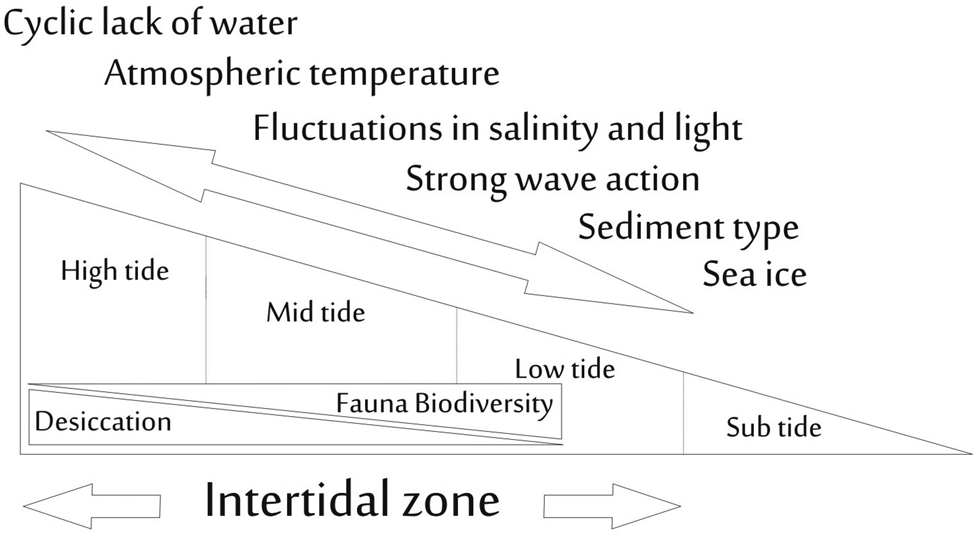
The Antarctic intertidal zone, similar to all intertidal zones worldwide, is a connector between the sea and land (Valdivia et al. Reference Valdivia, Scrosati, Molis and Knox2011, Chappuis et al. Reference Chappuis, Terradas, Cefalì, Mariani and Ballesteros2014, Griffiths & Waller Reference Griffiths and Waller2016). It is exposed, to a greater degree than the shallow subtidal zone, to changes in environmental conditions that take place in both realms, including water and air temperatures or predation from both terrestrial and marine organisms (Waller et al. Reference Waller, Barnes and Convey2006a, Reference Waller, Worland, Convey and Barnes2006b). Additionally, it is exposed to extremely severe environmental conditions, such as sea-ice presence, which do not occur at lower latitudes (Fig. 1) (Gutt Reference Gutt2001, Barnes & Conlan Reference Barnes and Conlan2007). The occurrence of intertidal fauna in the Antarctic was thought to be restricted due to the occurrence of ice cover, the abrasive action of ice or ice foot and the reduction of incoming solar radiation during winter (Bick & Arlt Reference Bick and Arlt2013). Seasonal changes in salinity caused by summer ice melting, runoff of mineral sediments and high ultraviolet radiation are considered additional reasons for poor settlement in the intertidal zones of polar regions (Bick & Arlt Reference Bick and Arlt2013). Due to freshwater runoff during the summer, Antarctic organisms may experience salinities as low as 12 or even lower when they are located in the centre of thawing. Furthermore, they are exposed to air temperatures that can vary by 20°C during a single tidal cycle (Barnes Reference Barnes1999, Gutt Reference Gutt2001, Waller et al. Reference Waller, Barnes and Convey2006a). This physical disturbance is considered an inherent part of ecosystems, and its intensity is crucial for shaping assemblage structures and biodiversity (Martín et al. Reference Martín, Miloslavich, Díaz, Ortega, Klein and Troncoso2016). Therefore, ice absence in large coastal areas of Antarctica during summer enables the development of diverse assemblages of intertidal invertebrates characterized by high succession dynamics (Siciński et al. Reference Siciński, Jazdzewski, de Broyer, Presler, Ligowski and Nonato2011, Martín et al. Reference Martín, Miloslavich, Díaz, Ortega, Klein and Troncoso2016).
Schematic model of the factors affecting the benthic faunal assemblages at different tidal zones.

Organism zonation in the intertidal region has a specific spatial arrangement (Chappuis et al. Reference Chappuis, Terradas, Cefalì, Mariani and Ballesteros2014). Vertical variations in species distributions usually reflect gradients or discontinuities of environmental conditions (Somero Reference Somero2002). The intertidal environment is a unique system because of strong physical gradients occurring across only a few metres from low to high altitudes (Valdivia et al. Reference Valdivia, Scrosati, Molis and Knox2011). A regular tidal cycle determines the time of exposure to air weather conditions, which increases with tidal height. For this reason, abiotic stressors such as temperature, desiccation, irradiation and osmotic potential increase towards the high tidal zone, where they reach their most extreme values (Menge & Branch Reference Menge, Branch, Bertness, Gaines and Hay2001, Valdivia et al. Reference Valdivia, Scrosati, Molis and Knox2011). In tropical or temperate areas, vertical zonation of organisms is very well understood, yet our knowledge of these mechanisms in Antarctica is still limited (Aghmich et al. Reference Aghmich, Taboada, Toll and Ballesteros2016, Martín et al. Reference Martín, Miloslavich, Díaz, Ortega, Klein and Troncoso2016, Marcías et al. Reference Marcías, Deregibus, Saravia, Campana and Quartino2017).
The aim of this study was to estimate the variability of invertebrate benthic fauna in the Antarctic intertidal zone of Admiralty Bay (King George Island, Antarctica) from an extremely low tidal water level to an extremely high spring tidal level. Although King George Island, due to its large number of research stations, is one of the most studied Antarctic regions, biodiversity in the intertidal zone remains poorly known (Bick & Arlt Reference Bick and Arlt2013). We examined the species richness, biomass and abundance of intertidal zone assemblages at a small spatial scale along and across the shoreline. Potential factors affecting the zonation of fauna in the study area are briefly discussed. The response of ecosystems to climate change is the most pressing problem in current and future Antarctic research (Kennicutt et al. Reference Kennicutt, Chown, Cassano, Liggett, Massom and Peck2014). Assuming that intertidal assemblages respond quickly to variations in environmental conditions and therefore reflect climate fluctuations, our study can potentially serve as a baseline study and reference for future more comprehensive research (Marcías et al. Reference Marcías, Deregibus, Saravia, Campana and Quartino2017).
Materials and methods
Study area
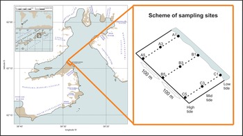
King George Island is the largest island in the South Shetland Archipelago, with an area of 1150 km2, of which > 90% is covered with ice. The island, ~100 km long and 25 km wide, is located 120 km north of the Antarctic Peninsula. The study area is located in Admiralty Bay, the largest fjord on the island and generally one of the largest fjords in this part of Antarctica (Fig. 2). The area is in the direct vicinity of the Arctowski Polish Antarctic Station. Although Admiralty Bay freezes at irregular intervals, the tidal zone is regularly covered with ice that can abrade the area in winter for several weeks or even months (Kuklinski & Balazy Reference Kuklinski and Balazy2014). The substrate of the tidal zone consists mainly of boulders, cobbles and pebbles overlying coarse sand and patches of solid rock with reflective foreshore slopes. The higher zone of the beach presents berm and beach ridges that are associated with the most significant storms and consist of gravel and pebbles.
Location of the sampling stations.

The tides have a regular daily character, and their amplitude is ~2 m (Catewicz & Kowalik Reference Catewicz and Kowalik1983). The annual surface seawater temperature ranges from -1.9°C to 3.8°C (Rakusa-Suszczewski Reference Rakusa-Suszczewski1995). Near the study area, the seawater temperature in the littoral zone ranges from 2.8°C to 3.8°C in summer and from 0.0°C to -1.7°C in winter (Jazdzewski et al. Reference Jazdzewski, Broyer, Pudlarz and Zielinski2001). Temperature variability is higher in summer, while in winter, due to the effect of ice buffering, the temperature is almost constant (Barnes Reference Barnes1999, Kuklinski & Balazy Reference Kuklinski and Balazy2014). The average salinity value in Admiralty Bay is 34.4 in winter and 33.5 in summer (Siciński et al. Reference Siciński, Jazdzewski, de Broyer, Presler, Ligowski and Nonato2011).
The temperature data used in this study were recorded at the same site and time by Kuklinski & Balazy (Reference Kuklinski and Balazy2014). They reported temperature fluctuations from -2.26°C (site B5) to 21.18°C (site B5), with an average value for all sites of 2.43°C. At each transect, the average temperature significantly increased with tidal height, from 1.79°C (site C1) and 1.91°C (site B1) in the low tidal zone to 2.93°C (site A5) and 4.10°C (site B5) in the high tidal zone.
Sampling procedure
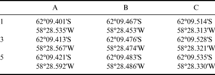
The sampling sites were located at low (LT), mid (MT) and high (HT) tidal levels at three transects perpendicular to the shoreline (A, B and C; see Fig. 2 & Table I). The distances between individual transects were 100 m, while the width between tidal heights was ~5 m. A 50 × 50 cm frame was used to collect macrofauna, while meiofauna samples were taken using a core with a diameter of 3.6 cm and a depth of 10 cm. Biological material was collected in January 2011 with three replicates taken for macrofauna (e.g. A1.1, A1.2 and A1.3) and five replicates taken for meiofauna (e.g. A1.1, A1.2, A1.3, A1.4 and A1.5) at each tidal altitude. Collected samples were preserved in a solution of 4% seawater-buffered formalin.
Coordinates of the sampling stations (A, B and C) at low (1), mid (3) and high (5) tidal levels. Location labels are according to Fig. 2.

Laboratory analyses
Macrofaunal (> 0.5 mm in size) organisms were picked, identified, counted and weighed. Most specimens were identified to the species level with the exception of early juvenile stages or significantly damaged individuals, which were identified to the lowest taxonomic level possible. Biomass is presented as a wet formalin weight for each taxon. Meiofauna (metazoan organisms that passed through the 500 μm sieve and were retained on the 38 μm sieve) were counted and sorted by taxa under a stereomicroscope.
Data analyses
The abundance of macrofauna and meiofauna (expressed as individuals per 0.25 m2 and 10 cm2, respectively), species/taxon richness, Shannon-Wiener's diversity index (H') and Pielou's evenness index (J') were determined for each sample (Clarke & Warwick Reference Clarke and Warwick1998). Quantitative data were square-root transformed, and the Bray-Curtis similarity coefficient was used and validated by the 'similarity profile' (SIMPROF) significance test (Clarke & Warwick Reference Clarke and Warwick2001). Additionally, individual species contributions to the observed clustering pattern were examined using 'similarity percentages' (SIMPER), a procedure that allows us to assess which species are principally responsible for the separation of the sets of samples (assemblage types) (Clarke & Warwick Reference Clarke and Warwick2001). K-dominance curves were constructed to detect shifts in dominance between tidal heights. A one-way analysis of similarities (ANOSIM) permutation test of the Bray-Curtis similarity data (Clarke & Warwick Reference Clarke and Warwick2001) was used to investigate differences in assemblage structure between different tidal heights and between individual transects. In ANOSIM, only tidal levels containing five or more records were taken into consideration. All statistical procedures were run in the PRIMER ver. 6.1.5. package (Clarke & Warwick Reference Clarke and Warwick2001). The significance level for all statistical tests used was P = 0.05.
Results
Macrofauna
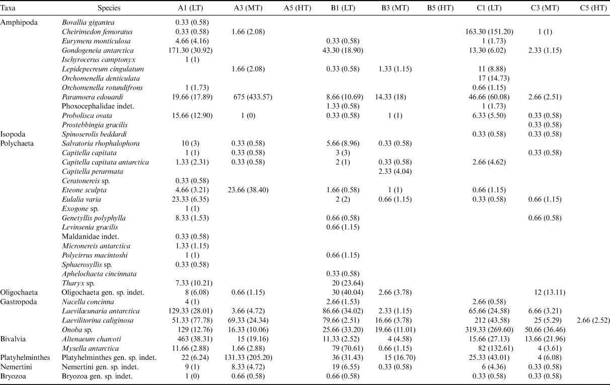
The studied material consisted of 11,057 individuals belonging to the following taxa: Amphipoda, Isopoda, Polychaeta, Oligochaeta, Gastropoda, Bivalvia, Platyhelminthes, Nemertini and Bryozoa (Table II). A total of 39 taxa were identified in 27 samples. Polychaetes and amphipods were the most diverse taxa, with 16 and 12 species recorded, respectively. Gastropods were represented by four species, followed by bivalves (two species). The remaining groups were represented by a single taxon. Seven samples (all replicates from stations A5 and B5 and sample C5.3; Table II) did not contain any macrofaunal organisms. The most numerous taxa were gastropods (3963 individuals, 36% of the total number), amphipods (3707 individuals, 34% of the total number) and bivalves (2105 individuals, 19% of the total number), whereas the least abundant taxa were isopods (two individuals).

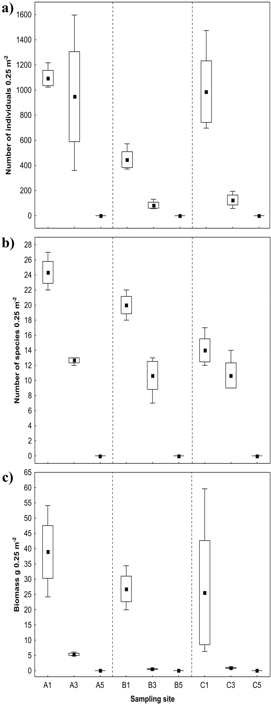
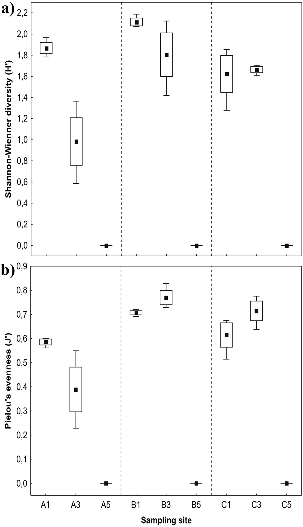
Macrofauna was most abundant in the LT zone (Fig. 3a), with an average number of individuals for all transects of 843 ± 373 ind. 0.25 m-2 (mean ± standard deviation). In the MT zone, 385 ± 525 ind. 0.25 m-2 were found, while in the HT zone, only 8 ± 1 ind. 0.25 m-2 were recorded. The most diverse was the LT zone (Fig. 3b), where the average species number was 19 ± 6 species 0.25 m-2. The MT zone was characterized by a lower mean species richness: 11 ± 2 species 0.25 m-2. The poorest species diversity was in the HT zone, with only one species recorded, the gastropod Laevilitorina caliginosa. The biomass values showed similar trends (Fig. 3c), with the highest mean value in the LT zone (30.40 ± 18.10 g 0.25 m-2), followed by the MT zone (2.25 ± 2.35 g 0.25 m-2) and the lowest in the HT zone (0.01 ± 0.008 g 0.25 m-2). The highest values of the Shannon-Wiener diversity index were at sites B1, A1 and B3, ranging from 1.81 to 2.11 (Fig. 4a), while Pielou's evenness index had the highest values at sites B3, C3 and B1, ranging from 0.71 to 0.77 (Fig. 4b).


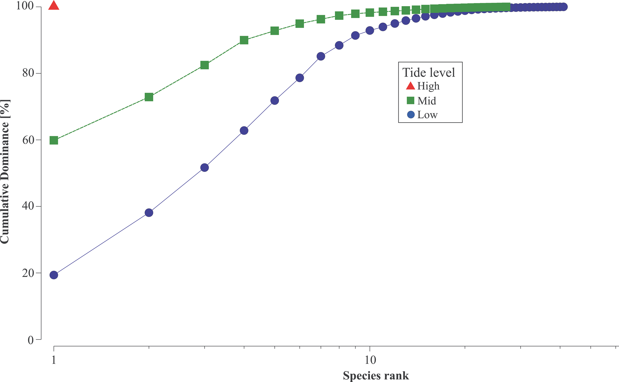
In general, assemblages occurring in the three different zones demonstrated a different dominance structure, as shown by the dominance curve (Fig. 5). The LT zone assemblage was more diverse, and the most dominant species accounted for only 20% of the total number of individuals within the assemblage. In the case of the MT zone, the dominant species had a turnout of 60% (Fig. 5), which contributed to less even shares of particular species at site A3 (Fig. 4b). In general, the number of species that characterized each zone decreased towards the HT zone: an abundance of six species contributed collectively to 80% of the assemblage in the lower zones, while the same level of cumulative dominance in the MT zone was contributed by only four species (Fig. 5).
Cumulative contribution of macrofaunal species to total community-wide similarity within each intertidal zone.

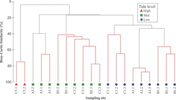
Cluster analysis separated samples into three groups: high, mid and low (Fig. 6). However, within these three major groups, six macrofaunal assemblages were identified (Fig. 6), as validated by the SIMPROF significance test (π = 0.5–4.4, P = 0.05). The first assemblage consisted of transect C samples (C1.1, C1.2 and C1.3) collected in the LT zone and featured 40% mutual similarity. These samples were numerically dominated by the gastropods L. caliginosa and Onoba sp. and the amphipod Cheirimedon femoratus at C1.1 and C1.2. The second cluster, including transect A samples (A1.1, A1.2 and A1.3), displayed a high mutual Bray-Curtis similarity of 80.57%. This assemblage also consisted of LT zone samples with high abundances of the bivalve Altenaeum charcoti and the crustacean Gondogeneia antarctica. The remaining LT samples of transect B (B1.1, B1.2 and B1.3) were grouped in the third assemblage. They were characterized by the presence of the similarly abundant gastropods Laevilacunaria antarctica and L. caliginosa and the less abundant amphipod G. antarctica. The fourth cluster comprised samples collected in the MT zone at transect A (A3.1, A3.2 and A3.3). This assemblage was dominated by an amphipod Paramoera edouardi, followed by the gastropods L. caliginosa and Onoba sp. The fifth assemblage contained samples collected in the same tidal zone at transects B and C, which were characterized by significantly lower abundances of macrofauna, with the molluscs L. caliginosa, Onoba sp. and L. antarctica as characteristic components. The last cluster consisted of samples C5.1 and C5.2 collected in the HT zone, containing only one species of the gastropod L. caliginosa (Fig. 6).

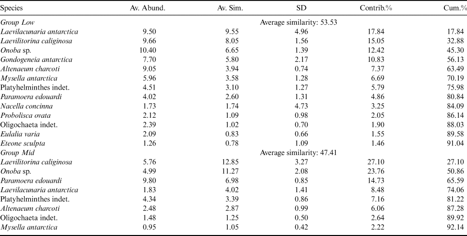
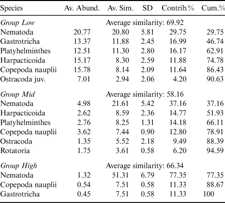
According to the ANOSIM test, there were significant differences between two tidal heights: the LT and MT levels (R = 0.678, P < 0.001). However, ANOSIM tests carried out for the transects (i.e. A, B and C) did not show any significant differences (R = 0.163, P = 0.062). All samples collected at low tide exhibited significantly higher abundances of macrofaunal species compared with less diverse and numerous samples from MT zone sites. The LT and MT zone groups were separated based on the frequency of the main species and their mutual proportions (indicated by SIMPER analysis; Table III). HT zone levels were not included in the analyses (ANOSIM, SIMPER) due to insufficient data.
Summary of 'similarity percentages' (SIMPER) results for macrofauna: average abundance (Av. Abund.; % cover) of typifying species in each zone and exposure group, average similarity (Av. Sim.), standard deviation (SD), their contribution (Contrib.%) to the within-group similarity and cumulative total (Cum.%) of contributions.

Meiofauna
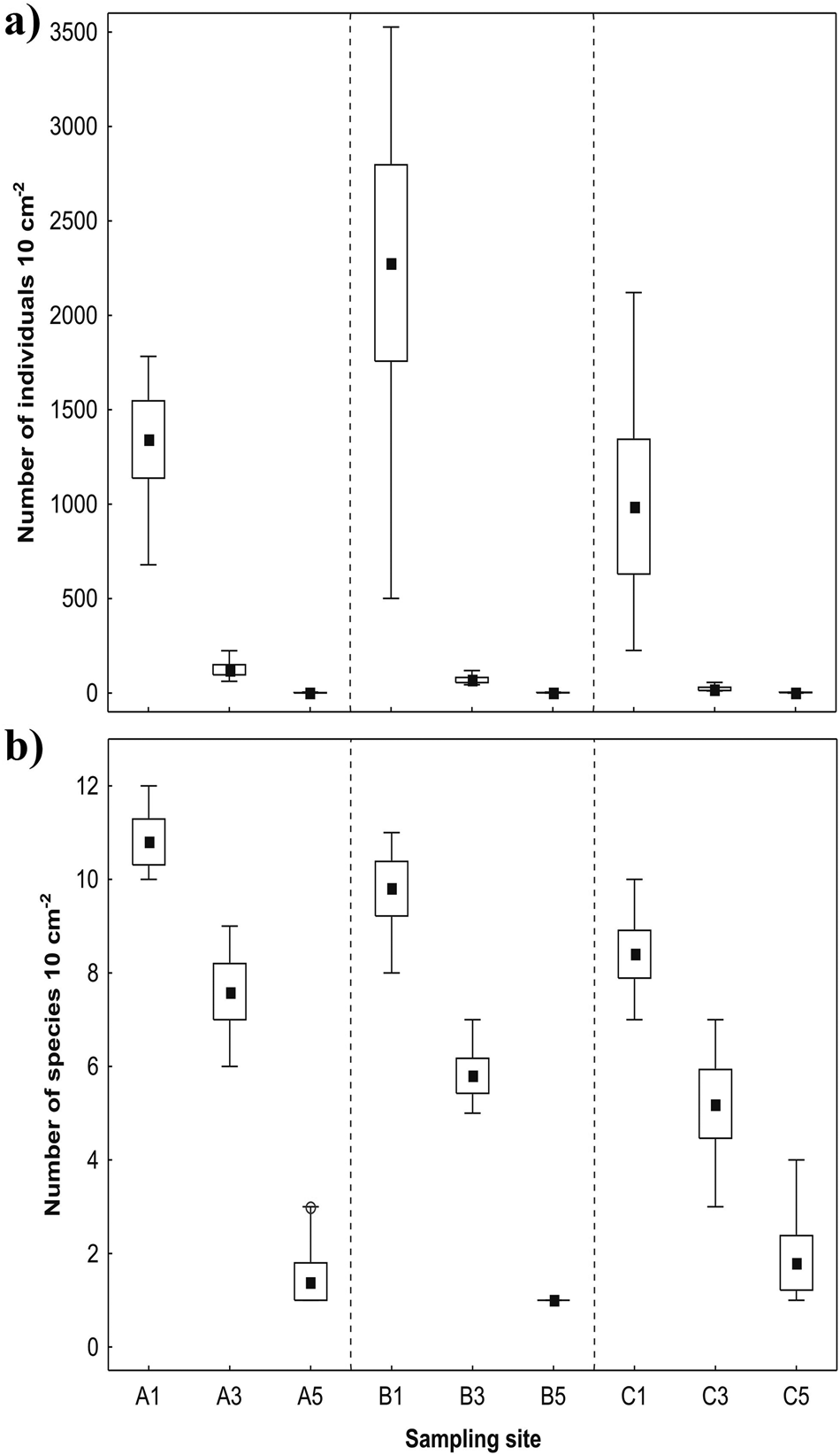
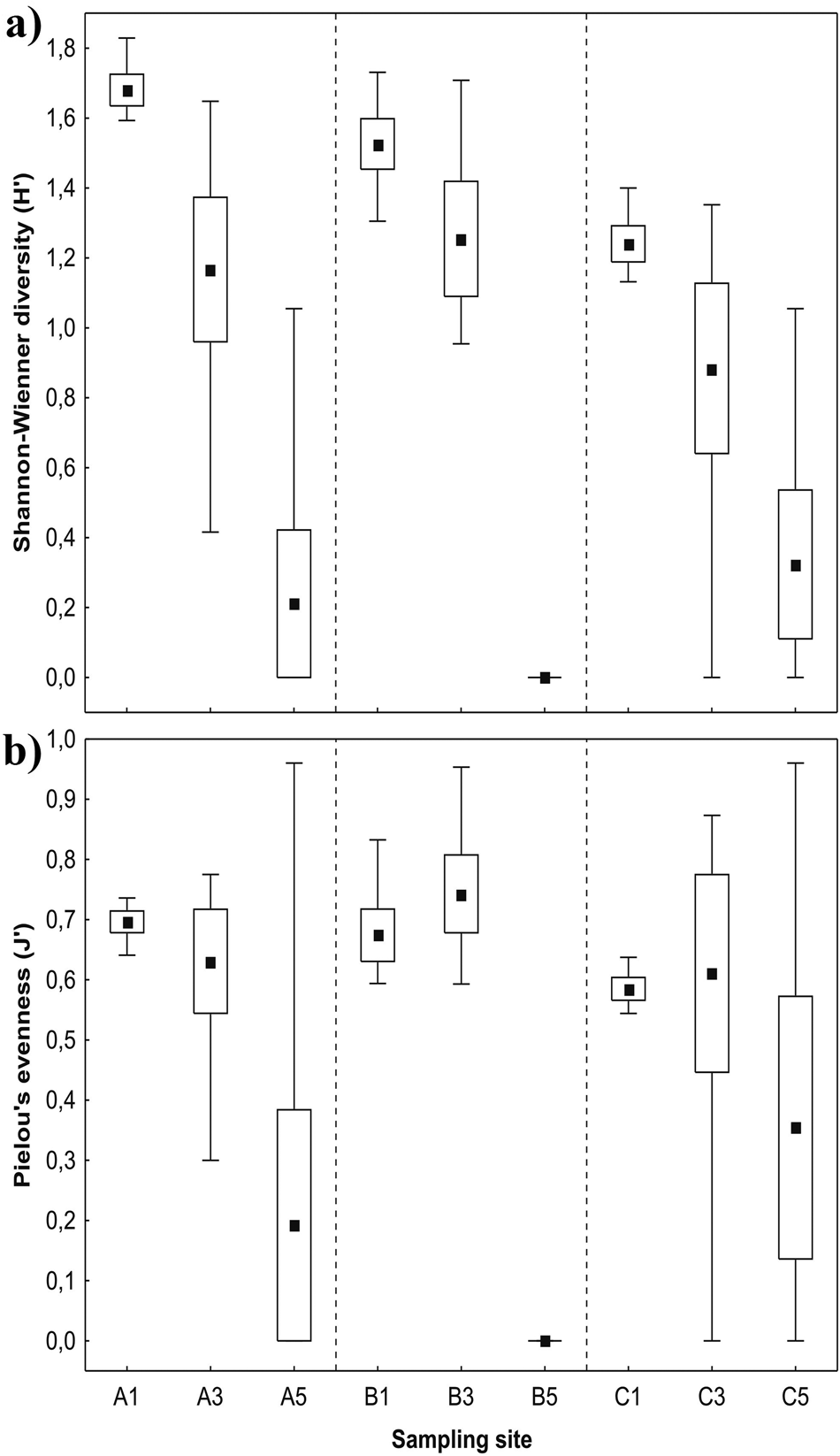
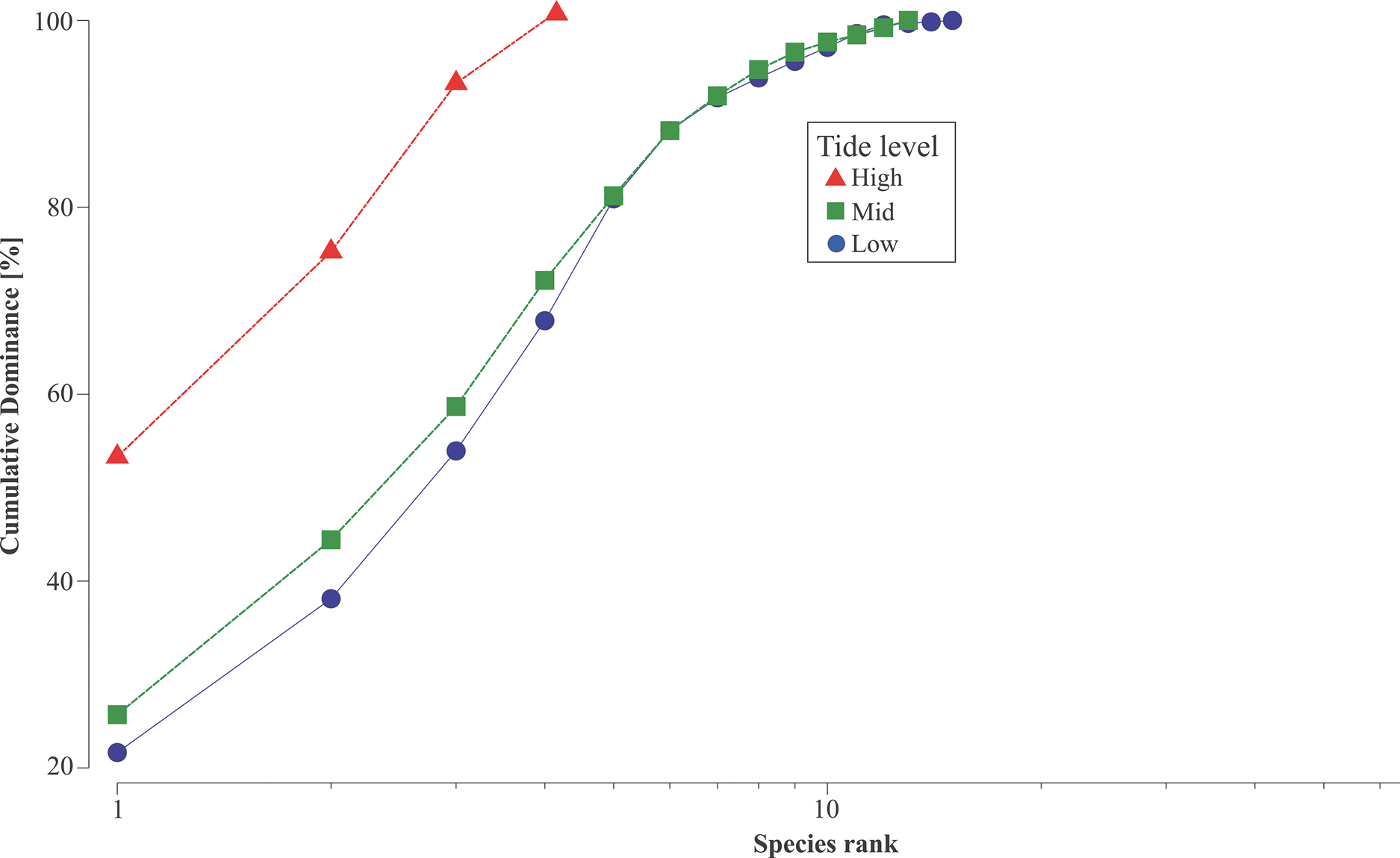
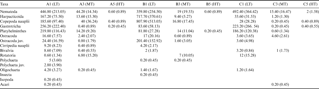
In total, 24,132 individuals belonging to 16 taxa (Table IV) were found in 45 samples. Juveniles accounted for 27.4% of the total number of collected individuals. Among all studied meiofaunal groups, the most numerous were nematodes (6908 individuals, 28.6% of the total number), copepod nauplii (5396 individuals, 22.4% of the total number) and harpacticoids (4714 individuals, 19.5% of the total number), whereas the least abundant taxa were Acari (two individuals) and Isopoda (single specimen). The highest average number of individuals for all transects was noted in the LT zone: 1536 ± 972 ind. 10 cm-2. Lower densities were observed in the MT zone (71 ± 57 ind. 10 cm-2), and the lowest was observed in the HT zone (1.86 ± 2 ind. 10 cm-2; Fig. 7a). Similarly, the highest number of taxa occurred in the LT zone (10 ± 1 taxa 10 cm-2), richness was lower in the MT zone (6 ± 2 taxa 10 cm-2) and the lowest number of taxa was found in the samples from the HT zone (1 ± 1 taxa 10 cm-2) (Fig. 7b). The highest values of the Shannon-Wiener diversity index were at sites A1, B1, B3 and C1, ranging from 1.24 to 1.68 (Fig. 8a). In the case of Pielou's evenness index, the highest values were at sites B3, A1, B1 and A3, ranging from 0.63 to 0.74 (Fig. 8b). These results were confirmed by the k-dominance curve (Fig. 9), which revealed a similar dominance structure of meiofaunal taxa in the LT and MT zones. Meiofauna assemblages from HT zone samples differed from the others due to the clear dominance of a single taxon (Nematoda, > 50%) and low total number of taxa noted (four taxa).


Cumulative contribution of meiofaunal taxa to total community-wide similarity within each intertidal zone.


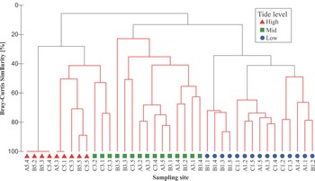
The separation of three major groups of samples in the cluster analysis (Fig. 10) was related to tidal height. The first cluster included samples from the HT and MT zones, with nematodes, followed by Gastrotricha and copepod nauplii, as the most numerous characteristic taxa (SIMPER analysis). The second cluster represented meiofaunal assemblages collected at low tide (A1, B1 and C1), and the SIMPROF test separated B1 from this group, which was the most numerous (Fig. 10). These samples were characterized by generally high numbers of individuals, with Nematoda, Gastrotricha, Platyhelminthes and Harpacticoida being particularly abundant (Table V). The same taxa, although at lower densities, along with sporadically noted Rotatoria, were important components in the third group of samples distinguished in the cluster (MT zone). The affinity of the samples was confirmed by the SIMPROF significance test (Fig. 10). ANOSIM confirmed statistically significant differences in meiofaunal diversity among LT, MT and HT zone samples (R = 0.82, P < 0.001), as well as among samples collected at the three transects (A, B and C; R = 0.733, P < 0.001).

Summary of 'similarity percentages' (SIMPER) results for meiofauna: abundance (Av. Abund.; % cover) of typifying species in each zone and exposure group, average similarity (Av. Sim.), standard deviation (SD), their contribution (Contrib.%) to the within-group similarity and cumulative total (Cum.%) of contributions.

Discussion
Based on our multidimensional approach using three sampling transects, we clearly showed that the largest variability in macrofauna and meiofauna diversity, abundance and biomass was present vertically across the shore. A strong decrease in all measured biodiversity indices was observed from the LT to the HT zones. Several abiotic parameters, such as duration of exposure to air (desiccation), wave action and temperature range, are known to shape zonation of the intertidal fauna across the globe (Valdivia et al. Reference Valdivia, Scrosati, Molis and Knox2011, Chappuis et al. Reference Chappuis, Terradas, Cefalì, Mariani and Ballesteros2014). In addition, some factors (e.g. permanent ice presence or ice coverage) are exceptional for polar areas (Griffiths & Waller Reference Griffiths and Waller2016). While the influence of all mentioned abiotic factors as a whole is very clear across the intertidal zones, the influence of a particular variable (e.g. desiccation) is hard to tease apart. It is generally accepted that physical settings are the main factor controlling the occurrence of organisms in the upper intertidal zones, while at lower tidal levels biotic interactions may have a larger impact (Davenport & Macalister Reference Davenport and Macalister1996, Martín et al. Reference Martín, Miloslavich, Díaz, Ortega, Klein and Troncoso2016), especially when organisms utilize the same potentially limited food source (Menge & Branch Reference Menge, Branch, Bertness, Gaines and Hay2001, Heaven & Scrosati Reference Heaven and Scrosati2008). In the case of Admiralty Bay, species richness and density were clearly highest in the LT zone; therefore, a higher intensity of interactions can be expected there than in less rich assemblages in the higher tidal zones. Biotic (e.g. predation and competition) influences on intertidal assemblages are still not fully understood, especially in the case of our study area. Kelp gulls (Larus dominicanus), a common member of the King George Island avifauna, actively feed intertidally, and this is a clear example of a biotic factor influencing this zone. Intense predation pressure by the gull significantly affects the population of the limpet Nacella concinna. Favero et al. (Reference Favero, Silva and Ferreyra1997), during a study at King George Island, reported that N. concinna was the main food item for the gulls, which spent 51% of their time searching for them. Overall, limpets are an important component of the kelp gull diet and supply 15–27% of their basic daily energy demand (Favero et al. Reference Favero, Silva and Ferreyra1997, Suda et al. Reference Suda, Vani, de Oliveira, Rodrigues, Rodrigues and Lavrado2015). Therefore, physical disturbance has an overwhelming impact on the assembly structure of Antarctic intertidal biological interactions and may also play some role in shaping the observed parameters of these biotopes.
Significant differences in faunal associations occurring in the three tidal levels between individual transects were noted only for meiofauna. Environmental factors probably act differently on meiofauna than on macrofauna. Habitat niches across the study area seem to be more homogeneous for macrofauna than for smaller organisms. For example, discrete differences in sediment properties may be an important factor regulating meiofauna occurrence and explaining the observed patterns. While sediments in transects A and C were mostly composed of coarse-grained sand, in transect B there was a higher admixture of fine-grained sand (personal observations). Coarse sediment is usually characterized by a lower organic content and higher porosity, which makes it less favourable to meiofaunal organisms (Veit-Köhler et al. Reference Veit-Köhler, Durst, Schuckenbrock, Hauquier, Durán Suja and Dorschel2018).
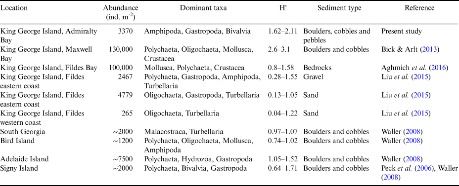
The abundance of Antarctic intertidal macrofauna can be very variable (Table VI). The highest densities reported for King George Island reached 130,000 ind. m-2 in the eastern part of the Fildes Peninsula (Bick & Arlt Reference Bick and Arlt2013). In the same intertidal area, Aghmich et al. (Reference Aghmich, Taboada, Toll and Ballesteros2016) found an invertebrate abundance reaching nearly 100,000 ind. m-2. Waller (Reference Waller2008) documented unexpectedly rich and abundant (~7500 ind. m-2) faunal associations in protected spaces between cobbles and under boulders on Adelaide Island. According to our results, density in Admiralty Bay (up to 3370 ± 1390 ind. m-2 in the lower zone; Table VI) is higher than those previously reported from Signy Island (2000 ind. m-2; Peck et al. Reference Peck, Convey and Barnes2006, Waller Reference Waller2008) and South Georgia and Bird islands (~2000 and ~1200 ind. m-2, respectively; Waller Reference Waller2008). It is also much higher than the values observed in the western part of the Fildes Peninsula (265 ind. m-2; Liu et al. Reference Liu, Wang, Li, Huo, He and Zhang2015). It has been documented that despite the harsh climate of the Antarctic Peninsula and Maritime Antarctic, tidal habitats can be much more diverse than at lower-latitude sites (Davenport & Macalister Reference Davenport and Macalister1996). The variability of macrofaunal density both within the Antarctic and in comparison to the sub-Antarctic results from many factors, including the geological history of a given area, physical settings or simple differences in bottom type (soft or hard bottomed; Hansom Reference Hansom and Schwartz2005). It is broadly accepted that reflective, coarser-grained beaches (especially gravel, cobble and boulder beaches) with steeper slopes are less favourable to intertidal organisms than dissipative, sandy beaches with gentler slopes (Aagaard et al. Reference Aagaard, Greenwood and Hughes2013). However, as our study shows, the Antarctic intertidal zone, with its coarser-grained sediments, has higher biodiversity values than sandy beaches (Table VI). Boulders and cobbles usually protect organisms more effectively from the influence of the extreme abiotic factors occurring in the Antarctic tidal zone, such as the destructive activity of sea ice, wind and wave action, fresh water runoff or ultraviolet radiation (Hansom Reference Hansom and Schwartz2005, Bick & Arlt Reference Bick and Arlt2013). Furthermore, macroalgal detritus trapped in sediment among hard structures can provide a food source for infauna. Generally, the multipronged structure of the intertidal zone can support a higher abundance and density of fauna than the soft sediments of flat tidal plains (Bick & Arlt Reference Bick and Arlt2013). Additionally, other disturbances (e.g. icebergs) may act very patchily on a given spot in the intertidal area, leading to differences in the biological structure of the compared areas. According to Waller (Reference Waller2008), long distances and the Polar Front oceanographically separate South Georgia from the northern cold temperate coasts. Furthermore, sub-Antarctic shores, but in particular those of South Georgia, are farthest from other polar tidal assemblages and therefore are away from a particular species pool, potentially leading to the impoverished nature of these assemblages.
Comparison of macrofaunal assemblages in the different Antarctic intertidal areas.

Our results showed that intertidal macrofauna are dominated by gastropods, followed by amphipods and less numerous bivalves. The same taxa dominate in the shallow sublittoral part of Admiralty Bay; however, Amphipoda dominates, followed by Gastropoda and Bivalvia (Jazdzewski et al. Reference Jazdzewski, Broyer, Pudlarz and Zielinski2001). Species recorded in the intertidal zone in the present study also occur in nearby shallow subtidal areas and are capable of adapting to unfavourable (adverse) environments. The most numerous species were gastropods: L. caliginosa and L. antarctica; amphipods: G. antarctica and P. edouardi; and a bivalve: A. charcoti. These organisms are eurybionts occurring from intertidal rocky shores to deeper subtidal depths (Siciński et al. Reference Siciński, Jazdzewski, de Broyer, Presler, Ligowski and Nonato2011). Similar to other polar regions, intertidal fauna of Admiralty Bay seem to be sourced from a nearby pool of shallow subtidal opportunistic organisms (Kuklinski & Barnes Reference Kuklinski and Barnes2008) and do not contain organisms unique to this zone only. The lack of specialized intertidal dwellers in the polar regions may be explained by an insufficient amount of time for tidal specialists to evolve, when life was 'suppressed' by the last glacial maximum and previous ice ages (Kuklinski & Barnes Reference Kuklinski and Barnes2008).
Based on the cluster analysis of the organisms, frequency distribution samples were clearly divided into the groups defined by the sampling area (LT, MT and HT zones; Fig. 6). Other studies have also reported similar divisions of the shore fauna (Schlacher & Thompson Reference Schlacher and Thompson2013, Marcías et al. Reference Marcías, Deregibus, Saravia, Campana and Quartino2017). Unsurprisingly, samples collected in the LT zone, where the level of environmental stress was lower than in the other zones, had the highest values of abundance, richness and diversity (Figs 3 & 4a). Some species important in the LT zone, such as the limpet N. concinna, did not occur at higher tidal levels. This species is known to be widespread and abundant in Antarctic shallow waters and plays a key role in creating tidal macrofaunal assemblages, species diversity and ecosystem stability (Liu et al. Reference Liu, Wang, Li, Huo, He and Zhang2015). In our material, N. concinna was not numerous but accounted for 70% of the total biomass. Similarly, a high dominance of limpets in biomass was reported from the LT zones of the Antarctic Peninsula (74%; Waller et al. Reference Waller, Barnes and Convey2006a) and the sub-Antarctic region (78%; Blankley & Grindley Reference Blankley, Grindley, Siegfried, Condy and Laws1985, Waller et al. Reference Waller, Barnes and Convey2006a). Despite its physiological flexibility (Suda et al. Reference Suda, Vani, de Oliveira, Rodrigues, Rodrigues and Lavrado2015), N. concinna cannot survive in higher tidal zones, where the temperature can reach up to + 21.18°C (Kuklinski & Balazy Reference Kuklinski and Balazy2014). Limpets have a range of adaptations to survive at higher temperatures, but biological functions important to the long-term existence of the species are strictly limited to a very narrow temperature range (Peck et al. Reference Peck, Webb and Bailey2004).
Macrofauna of the MT zone were dominated by a single species, the amphipod P. edouardi (Figs 4b & 5). This species is very abundant in the intertidal zone during summer, probably due to the availability of a rich food source: algal detritus produced by the rich subtidal algal assemblage and often scattered across the intertidal zone at different tidal heights (Jazdzewski et al. Reference Jazdzewski, Broyer, Pudlarz and Zielinski2001). Fragmentation and decomposition last a few weeks, and a third of this algal biomass is released as detritus and nutrients (Zieliński Reference Zieliński1981). Jazdzewski et al. (Reference Jazdzewski, Broyer, Pudlarz and Zielinski2001) concluded that organism density in the uppermost sublittoral zone, which is at the border of the intertidal zone, changes throughout the year depending on the appearance of macroalgae. These authors observed dense clusters of amphipods and gastropods during summer from January to February.
In the HT zone, which is exposed to the most adverse environmental conditions, only one taxon occurred with low density and biomass. A low abundance of macrofauna in this zone is common not only at high latitudes but also at lower latitudes (Menge & Branch Reference Menge, Branch, Bertness, Gaines and Hay2001). For example, Menge et al. (Reference Menge, Daley, Lubchenco, Sanford, Dahlhoff and Halpin1999) reported a very low number of barnacles (5 ind. per 100 cm2) in this zone in New Zealand, and Bertness et al. (Reference Bertness, Crain, Silliman, Bazterrica, Reyna, Hildago and Farina2006) noted that the HT zone habitat on the Patagonian coast of Argentina was dominated by bare space (> 85%), with only one species occurring. The species found in this study was the opportunistic and abundant shallow-water gastropod L. caliginosa (Arnaud et al. Reference Arnaud, Jazdzewski, Presler and Sicinski1986, Jazdzewski et al. Reference Jazdzewski, Broyer, Pudlarz and Zielinski2001). It is the most common littorinid in the Antarctic and sub-Antarctic regions and is known for its significant thermal tolerance ranging from -11°C to +28°C (Davenport & Macalister Reference Davenport and Macalister1996). This species can survive in the harsh conditions of the Antarctic HT zone due to its unique biological adaptations, such as its strong shell sculpture for convective heat loss, the reduction in relative size of the aperture and its attachment to the substratum by a film of mucus when the operculum is closed (Reid Reference Reid1989).
Both the densities and taxonomic composition of the intertidal meiofauna of Admiralty Bay were similar to those observed in other climatic zones and marine environments. The present material was dominated by Nematoda, followed by Copepoda nauplii and Harpacticoida, which is in agreement with previous studies (e.g. de Skowronski & Corbisier Reference De Skowronski and Corbisier2002, Kotwicki et al. Reference Kotwicki, De Troch, Urban-Malinga, Gheskiere and Weslawski2005a). It is well known that nematodes have an amazing ability to adapt to different environmental conditions (Lee & Van de Velde Reference Lee, Van de Velde, Arntz and Gutt1999), and their abundance was recorded even up to 14,943 ind. 10 cm-2 (85.9% of the total) in the intertidal muddy sediment at locations such as the sub-Antarctic Kerguelen Islands (49°S, 70°E; Bouvy & Soyer Reference Bouvy and Soyer1989). In our material, nematodes dominated numerically at most study stations but had a moderate share of the total meiofaunal abundance (30%). The relatively low proportion of nematodes within the meiofaunal assemblages was probably related to coarse-grained sediment forming larger interstitial spaces that favour the occurrence of other meiofaunal taxa (Urban-Malinga et al. Reference Urban-Malinga, Wiktor, Jabłońska and Moens2005). Overall, sediment granulometry significantly influences the vertical distribution pattern of nematode assemblages in sediments. In well-oxygenated, coarse-grained sediments, the nematode abundance on the surface remains generally lower and increases considerably with depth (Steyaert et al. Reference Steyaert, Vanaverbeke, Vanreusel, Barranguet, Lucas and Vincx2003). Alternatively, it is possible that environmental conditions occurring in polar intertidal environments (e.g. ice scouring, sediment turnover, salinity and temperature variability) may exceed the adaptability of nematodes (Urban-Malinga et al. Reference Urban-Malinga, Wiktor, Jabłońska and Moens2005). Copepod nauplii and harpacticoids were another important group in our study, making up 22% and 19% of the total meiofaunal abundance, respectively. Bick & Arlt (Reference Bick and Arlt2013) in Maxwell Bay noted a higher percentage of harpacticoids in fine sand (41%) than in coarse sand (32%). According to published information, their density is strongly regulated by food input to the system (Vanhove et al. Reference Vanhove, Beghyn, Van Gansbeke, Bullough and Vincx2000). This is another positive correlation between sediment properties (utilizable organic matter and fine-grained sand) and meiofaunal abundance (Delgado et al. Reference Delgado, Riera, Monterroso and Núnez2009).
The patterns of meiofaunal distribution were similar to those observed for macrobenthos. Three major groups of meiofaunal assemblages typical for each tidal zone were distinguished in the cluster analysis (Fig. 10). Meiofauna of the LT zone was the most abundant, species rich and diverse, while the HT zone was the most impoverished (Figs 7 & 8a). The average density at low tide noted in this study (1535 ± 972 ind. 10 cm-2) was higher than that reported by Bick & Arlt (Reference Bick and Arlt2013) in the intertidal zone of nearby Maxwell Bay (53.3 ind. 10 cm-2). Differences in abundance may result from sample sizes, the different distances from sea level, the physical dynamics of these locations and the patchy distribution of food. In Admiralty Bay, large quantities of macroalgae are deposited on the beach, supporting organisms that feed on bacteria associated with decaying macroalgae (Zieliński Reference Zieliński1981). The MT zone had a similar taxon contribution as the LT zone, without the dominant taxon (Fig. 9). These results were also confirmed by the values of Pielou's evenness index, which indicated that the abundance distribution of the different taxa in the MT zone was homogeneous (Fig. 8b). Similarly, a low number of organisms was noted by Kotwicki et al. (Reference Kotwicki, Szymelfenig, De Troch, Urban-Malinga and Węsławski2005b), who found 35 ind. 10 cm-2 in the MT zone on a sandy beach in Admiralty Bay, which is consistent with our results (71 ± 57 ind. 10 cm-2). This pattern could be the result of vertical migrations within the sediment. As exposure to air is longer in the MT zone than in the LT zone, meiofauna could migrate to deeper, more stable environmental layers of sediment to avoid desiccation. According to Gheskiere et al. (Reference Gheskiere, Vincx, Weslawski, Scapini and Degraer2005), physical disturbances (exposure to atmospheric conditions) may affect the vertical distribution of meiofauna, which might also be the case in our study area. McLachlan et al. (Reference McLachlan, Erasmus and Furstenberg1977) reported that meiofauna migrate downwards at low tide and upwards at high tide, while the range of the depth distribution of meiofauna on well-oxygenated beaches could potentially reach up to 50 cm and deeper.
Conclusions
Despite the past general view that Antarctic intertidal zones are unfavourable for life because of harsh polar conditions, recent and current studies confirm that intertidal assemblages can survive in this extreme environment. This study described the density and diversity patterns of macrofauna and meiofauna at a given time, providing baseline information for future research. We discovered species-rich and thriving assemblages whose occurrence and abundance seem to be governed by similar factors to those from lower latitudes, including, among many, biological adaptation of species to desiccation, temperature changes or wave action. With respect to rapidly ongoing global warming and glacial retreat, new ice-free areas will be created and become available for colonization. Moreover, with increasing air temperature, and therefore sea water temperature, the intertidal zone, which is the interface between marine and terrestrial systems, is most probably one of the first areas to be influenced by warming. We therefore recommend adopting intertidal zones as model systems to investigate the effects of climate change and to conduct long-term monitoring. Assuming that intertidal fauna quickly respond to changes in environmental conditions, continuous monitoring of this zone can provide information on the distribution of species in response to progressing climate change. To fully understand the complexity of intertidal systems, future research should be conducted along environmental gradients at broader spatial scales. Knowledge of the spatial and temporal context in which repetitive patterns occur can significantly increase the accuracy and precision of ecological forecasts.
Acknowledgements
We would like to address special thanks to Tadeusz Stryjek for help during each step of the expedition. We would also like to thank Andrzej Tatur, Tomasz Janecki and Anna Kidawa for help with the expedition organization. Jaroslaw Roszczyk, Mateusz Bagnicki, Lech Wisniewski and the rest of the Arctowski Polish Antarctic Station crew, including Kazimierz Połeć, Tadeusz Markowicz, Wiesław Sienkiewicz, Kazimierz Warowicki, Włodzimierz Tkaczyk, Waldemar Kowalski, Michał Guźniczak and Piotr Horzela, are thanked for their help with logistics and for being great company during the fieldwork. Two anonymous reviewers are thanked for comments and corrections leading to an improved manuscript.
Financial support
This research was finished thanks to funding provided by grant PANIC/2016/23/B/ST10/01936 to PK from the National Science Centre Poland.
Author contributions
PK designed and provided funds for the study. PK and PB conducted sample collection. MC, KG, LG, MK and JL conducted taxonomic identification. MC prepared the original draft, which was reviewed and edited by all co-authors.