1 Introduction
Wall-bounded turbulence, particularly at high Reynolds number, is important in a wide range of practical flows. Three examples (commonly called the canonical flows) are pipe, channel and zero streamwise pressure gradient boundary layer flows above smooth walls. While the canonical flows are common in a wide range of applications, for the majority of practical flows the bounding wall has surface topography that exerts a dynamical effect on the flow. Herein and in the literature, surfaces with dynamically significant perturbations are referred to as rough walls. Rough-wall-bounded flows include, but are by no means limited to, geophysical flows such as the atmospheric and benthic boundary layer, boundary layers developing on marine and terrestrial vehicles and flows in piping networks. A characteristic feature of these applications is the large span of Reynolds numbers they cover. Therefore, understanding the Reynolds number scaling of rough-wall flows is central to their accurate prediction. Even in the canonical flow cases, however, sufficient understanding of the flow dynamics has been elusive despite decades of research. There is much to be learnt generally about wall-bounded flows from examination of boundary layers subjected to perturbations such as wall roughness (for example, in understanding the relative importance, dynamics and interactions of the inner and outer scales – see Abe, Kawamura & Choi Reference Abe, Kawamura and Choi2004; Toh & Itano Reference Toh and Itano2005; Hutchins & Marusic Reference Hutchins and Marusic2007a ,Reference Hutchins and Marusic b ).
1.1 Scaling and similarity hypotheses
Roughness manifests over a range of geometries and sizes. It is therefore useful to have a means for comparing different roughnesses. For most roughness types – ‘
 $k$
-type’ roughness (see Perry, Schofield & Joubert Reference Perry, Schofield and Joubert1969) – this is commonly provided in the form of an equivalent sand grain roughness Reynolds number,
 $k_{s}^{+}$
, where
 $k_{s}^{+}=k_{s}U_{{\it\tau}}/{\it\nu}$
(
 $U_{{\it\tau}}$
is the friction velocity and
 ${\it\nu}$
is the kinematic viscosity). As in smooth-wall flows, the inner-normalised mean streamwise velocity over a rough wall exhibits a region of log-linear dependence, with the same slope but with the additive constant being shifted vertically downward by
 ${\rm\Delta}U^{+}$
, the roughness function. This shift is due to the increased drag of the rough surface; in rough-wall flows there is a drag contribution from both viscous and pressure forces. Because
 $k_{s}^{+}$
depends on
 ${\rm\Delta}U^{+}$
, it can be used to characterize the rough-wall drag increment relative to the smooth wall, relating flows of geometrically different roughnesses through this net effect. At high roughness Reynolds number the viscous component of the surface drag is negligible compared with the pressure drag of the roughness elements and the flow is conventionally termed ‘fully rough’. For fully rough flows there is a log-linear relationship between
 $k_{s}^{+}$
and
 ${\rm\Delta}U^{+}$
(Nikuradse Reference Nikuradse1933). Conversely, at very low roughness Reynolds numbers, the wall roughness has negligible effect on the viscous sublayer (
 ${\rm\Delta}U^{+}\rightarrow 0$
), and the flow is ‘dynamically smooth’. At intermediate roughness Reynolds numbers where the near-wall flow is influenced by both pressure and viscous drag, the flow is referred to as ‘transitionally rough’. Flows are commonly considered to be hydraulically smooth for
 $k_{s}^{+}\lesssim 4$
, and fully rough above
 $k_{s}^{+}\approx 70$
, although these bounds are only approximate (Ligrani & Moffat Reference Ligrani and Moffat1986; Jiménez Reference Jiménez2004).
Experimental data exist for a range of roughness geometries across the transitionally and fully rough regimes. Reviews of the rough-wall turbulent flow literature are given by Raupach, Antonia & Rajagopalan (Reference Raupach, Antonia and Rajagopalan1991) and more recently by Jiménez (Reference Jiménez2004). One conclusion of both reviews is that the majority of experimental and computational evidence provides support for what is commonly referred to as Townsend’s wall-similarity hypothesis. The hypothesis, termed Reynolds number similarity by Townsend (Reference Townsend1956), implies that at high Reynolds numbers, a ‘fully turbulent’ flow is unaffected by viscosity, except through the boundary conditions (a region where the direct influence of viscosity is negligible is congruous with an inertial region of the flow). On rough-wall-bounded turbulence, Townsend writes:
At distances from the wall large compared with the extent of the flow patterns set up by individual roughness elements, the turbulent flow is unlikely to be affected by the exact nature of the roughness and, as with the smooth wall, it will be determined by the averaged wall stresses, the channel width [or in boundary layers,
 ${\it\delta}$
, the boundary layer thickness] and the fluid viscosity.
In the literature, numerous roughness studies lend support for Townsend’s hypothesis in boundary layer (e.g. Raupach Reference Raupach1981; Flack, Schultz & Shapiro Reference Flack, Schultz and Shapiro2005; Volino, Schultz & Flack Reference Volino, Schultz and Flack2007), pipe (e.g. Shockling, Allen & Smits Reference Shockling, Allen and Smits2006; Allen et al.
Reference Allen, Shockling, Kunkel and Smits2007; Hultmark et al.
Reference Hultmark, Vallikivi, Bailey and Smits2013) and channel flows (e.g. Flores & Jimenez Reference Flores and Jimenez2006; Hong, Katz & Schultz Reference Hong, Katz and Schultz2011). There are, however, a number of studies that report a lack of similarity between smooth- and rough-wall outer-layer flows (e.g. Krogstad, Antonia & Browne Reference Krogstad, Antonia and Browne1992; Tachie, Bergstrom & Balachandar Reference Tachie, Bergstrom and Balachandar2000; Keirsbulck et al.
Reference Keirsbulck, Labraga, Mazouz and Tournier2002; Leonardi et al.
Reference Leonardi, Orlandi, Smalley, Djenidi and Antonia2003; Bhaganagar, Kim & Coleman Reference Bhaganagar, Kim and Coleman2004; Lee & Sung Reference Lee and Sung2007). Jiménez (Reference Jiménez2004) asserts that the conflicting findings with regard to Townsend’s hypothesis may simply be the result of the large relative roughness height,
 $k/{\it\delta}$
, that has been employed in a number of studies. When
 $k/{\it\delta}$
is large, the region of the flow directly influenced by the roughness may occupy a significant fraction of the boundary layer. This notionally defined region is called the roughness sublayer and has been suggested to extend a few roughness heights above the roughness (Raupach et al.
Reference Raupach, Antonia and Rajagopalan1991; Flack, Schultz & Connelly Reference Flack, Schultz and Connelly2007). Jiménez (Reference Jiménez2004) concludes that a set of well-characterized experiments in the fully rough flow regime is required to clarify the validity of Townsend’s hypothesis. He contends that these experiments should be carried out in flows in which the equivalent sand grain roughness is high (
 $k_{s}^{+}>100$
), and the relative roughness height is small (
 ${\it\delta}/k\gtrsim 40$
), suggesting that the friction Reynolds number,
 ${\it\delta}^{+}={\it\delta}U_{{\it\tau}}/{\it\nu}$
, must be at least
 $4000$
, for both requirements to be simultaneously satisfied. Some studies, however, imply that the relative roughness height must be at least
 ${\it\delta}/k\gtrsim 130$
for wall similarity to be observed (Efros & Krogstad Reference Efros and Krogstad2011), shifting the limiting
 ${\it\delta}^{+}$
to over
 $10\,000$
. Note that Jiménez (Reference Jiménez2004) also compiles transitionally rough data from previous studies and from this concludes that there is a similar need for measurements in transitionally rough flows that have a low relative roughness height. In this paper, data are presented across a wide range of roughness and friction Reynolds numbers, targeting these regimes identified by Jiménez (Reference Jiménez2004) as being sparsely populated by pre-existing data.
1.2 Measuring wall shear stress
A pertinent issue confounding the empirical analysis of rough-wall flows is the difficulty in accurately estimating the mean wall shear stress,
 ${\it\tau}_{w}$
. Aside from its obvious importance in assessing the drag due to the rough wall, the wall shear stress is required to compute the friction velocity,
 $U_{{\it\tau}}=\sqrt{{\it\tau}_{w}/{\it\rho}}$
, which is a fundamental scaling parameter in wall-bounded turbulent flows (note that
 ${\it\rho}$
is the fluid density). The ubiquitous challenges associated with determining
 ${\it\tau}_{w}$
have been discussed by a number of researchers (e.g. Perry et al.
Reference Perry, Schofield and Joubert1969; Acharya, Bornstein & Escudier Reference Acharya, Bornstein and Escudier1986; Brzek et al.
Reference Brzek, Cal, Johansson and Castillo2007; Walker Reference Walker2014). The vast majority of rough-wall boundary layer studies rely on similarity in either the inner or outer layer to determine
 ${\it\tau}_{w}$
. This is obviously not desirable in studies aiming to assess wall similarity, and is, to a certain degree, a circular argument. There are only a few notable examples of rough-wall boundary layer experiments that independently determine
 ${\it\tau}_{w}$
. Mulhearn & Finnigan (Reference Mulhearn and Finnigan1978), Acharya et al. (Reference Acharya, Bornstein and Escudier1986) and Krogstad & Efros (Reference Krogstad and Efros2010), for example, use a force balance to directly measure the average wall shear stress on a small sensing element. Brzek et al. (Reference Brzek, Cal, Johansson and Castillo2007) evaluated the momentum integral equation to determine the shear stress on a rough wall. However, the use of the momentum integral equation requires the streamwise evolution of the boundary layer to be documented, which is uncommon in the literature. In the following we present experimental results based on
 $U_{{\it\tau}}$
measurements obtained from a purpose built drag balance. As described recently by Baars et al. (Reference Baars, Squire, Talluru, Abbassi, Hutchins and Marusic2016), these are capable of higher accuracy than previous measurements, with an estimated uncertainty of
 ${<}2.5\,\%$
.
1.3 Outline of paper
Streamwise velocity statistics and spectral intensities are presented for rough-wall turbulent boundary layers over the range
 $3000\lesssim {\it\delta}_{99}^{+}\lesssim 30\,000$
. Herein,
 ${\it\delta}_{99}$
denotes the wall-normal location at which the mean streamwise velocity is
 $99\,\%$
of the free stream velocity,
 $U_{\infty }$
. Only results from hot-wire anemometry (HWA) sensors are presented in this paper, although particle image velocimetry measurements were also acquired (to be detailed in a later paper). The measurements are unique in that they span nearly a decade in Reynolds number while maintaining good spatial and temporal resolution. Two sets of experiments are presented. The first was taken at two streamwise locations at which the free stream velocity was varied to generate a wide Reynolds number range. A subset of these experiments used the force balance to directly measure
 ${\it\tau}_{w}$
. These measurements span the transitional and fully rough regimes, all with a very small relative roughness (
 ${\it\delta}_{99}/k_{s}>120$
). The second set of measurements documents the spatial development of the fully rough, rough-wall boundary layer from low to high Reynolds number over a fetch of nearly 22 m. Spatially developing rough-wall boundary layer data are obtained at four free stream velocities. At the highest velocity, the data are all fully rough (
 $k_{s}^{+}>100$
) and cover a wide range of relative roughness heights (
 $28<{\it\delta}_{99}/k_{s}<198$
). Smooth-wall data (present; Marusic et al.
Reference Marusic, Chauhan, Kulandaivelu and Hutchins2015; Morrill-Winter et al.
Reference Morrill-Winter, Klewicki, Baidya and Marusic2015) measured in the same facility at Reynolds numbers that approximately match those in the present rough-wall experiments, provide comparisons. Throughout this paper,
 $x$
,
 $y$
and
 $z$
denote the streamwise, spanwise and wall-normal directions, respectively, with
 $z=0$
located at the roughness crest. Uppercase variables are mean quantities and lowercase variables denote fluctuations. A ‘
 $+$
’ superscript indicates inner normalisation (i.e. using
 ${\it\nu}$
and
 $U_{{\it\tau}}$
).
2 Experimental conditions and procedures
2.1 Facility
The experiments were performed in the High Reynolds Number Boundary Layer Wind Tunnel (HRNBLWT) at the University of Melbourne. In this open-return blower facility, a turbulent boundary layer develops on the floor of the 0.92 m
 $\times$
1.89 m
 $\times$
27 m working section. Details of the facility are available in Nickels et al. (Reference Nickels, Marusic, Hafez and Chong2005, Reference Nickels, Marusic, Hafez, Hutchins and Chong2007). Measurements were made above a smooth and rough wall, between 1.6 m and 21.7 m downstream of the laminar/turbulent trip. For the smooth-wall measurements, the tunnel floor was constructed from five polished aluminium plates with a root-mean-squared surface roughness less than
 $15~{\rm\mu}\text{m}$
(at most 1.2 wall units for the measurements presented here). For all measurements above the rough wall, the floor of the working section was covered with sandpaper. Details of the sandpaper roughness and its installation are provided in § 2.2. The free stream velocity variation along the entire working section was checked at 20, 30 and
 $40~\text{m}~\text{s}^{-1}$
above the smooth wall, and at 10 and
 $20~\text{m}~\text{s}^{-1}$
above the rough wall and was less than
 $\pm 0.50\,\%$
for all cases. The floating element drag balance is a large flat plate of dimensions 3 m
 $\times$
1 m, mounted between 19.5 and 22.5 m downstream of the laminar/turbulent trip. Four air bearings allow for almost frictionless streamwise movement of the plate. Because the surface area of the drag balance is large, the shear force measurement has a uniquely high signal-to-noise ratio (
 ${>}25$
). See (Baars et al.
Reference Baars, Squire, Talluru, Abbassi, Hutchins and Marusic2016) for further details of the floating element drag balance.
2.2 Surface roughness
For the rough-wall measurements, the entire floor of the wind tunnel working section was covered with P36 grit sandpaper (SP40F, Awuko Abrasives). With the exception of the drag balance measurements, all rough-wall measurements were performed above a single 1.82 m
 $\times$
28 m sheet of sandpaper. The sheet was affixed to the tunnel floor at the trip using four spanwise strips of double-sided tape. At the tunnel exit, the sheet passed over a pulley that spanned the full tunnel width, and was weighted using two 20 kg free-hanging masses. As such, the sheet was in tension for the duration of the measurements. This removed undulations in the sandpaper sheet that formed when the sheet was not in tension. During drag balance measurements, multiple sandpaper sheets were used to allow for unrestricted movement of the floating element (see Baars et al.
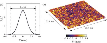
Reference Baars, Squire, Talluru, Abbassi, Hutchins and Marusic2016). A Veeco Wyco NT9100 optical profilometer was used to quantify the surface parameters of the sandpaper over a 25.4 mm
 $\times$
25.4 mm area (results given in figure 1
b). This apparatus utilizes white light interferometry and has submicron vertical accuracy. Figure 1(a) shows the probability density function (p.d.f.) of roughness surface elevation. Note that the distribution of roughness heights for the sandpaper surface is approximately normally distributed. Here, the physical roughness height of the sandpaper surface is defined as
 $k=6{\it\sigma}=0.902~\text{mm}$
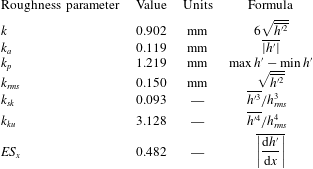
. Key roughness surface parameters are presented in table 1.
Details of the sand grain surface roughness obtained by scanning a 25.4 mm
 $\times$
25.4 mm section of the sandpaper. In (a), the solid black line shows a p.d.f. of the surface elevation about the mean sand grain height, while the dashed purple line shows a normal distribution. (b) Shows the scan of the sandpaper section.

The roughness function,
 ${\rm\Delta}U^{+}$
, as a function of the inner-normalised roughness height,
 $k_{s}^{+}$
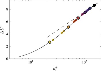
. Symbols with black outlines show the Case 1 rough-wall data at 21.7 m, for which
 $U_{{\it\tau}}$
is determined directly from the drag balance measurements; the solid grey line is a smoothing spline fit to a cubic interpolation of the Case 1 rough-wall data at 21.7 m. The dashed black line shows the fully rough asymptote of Nikuradse (Reference Nikuradse1933). All symbols are defined in table 2.

Key surface parameters from the scanned surface data, where
 $h^{\prime }$
is the surface deviation about the mean height (
 $h^{\prime }=h-\overline{h}$
).

Figure 2 presents the roughness function dependence on the equivalent sand grain roughness for all of the rough-wall data. The data outlined in black were taken above the drag balance, enabling
 $U_{{\it\tau}}$
to be determined directly. The method used to determine
 $U_{{\it\tau}}$
for the remaining rough-wall data is described in § 2.4. The roughness function is chosen for each dataset to minimise the least-squares error between the inner-normalised streamwise velocity profile and the rough-wall logarithmic law,
 $$\begin{eqnarray}\displaystyle U^{+}=\frac{1}{{\it\kappa}}\log (z+{\it\epsilon})^{+}+A-{\rm\Delta}U^{+}, & & \displaystyle\end{eqnarray}$$
across the inertial sublayer. The wall-normal bounds of the inertial sublayer and the wall correction parameter
 ${\it\epsilon}$
are discussed in § 2.4. Note, however, that
 ${\rm\Delta}U^{+}$
is largely insensitive to changes in the start and end locations of the inertial sublayer; changing either location by
 $\pm 15\,\%$
causes
 ${\rm\Delta}U^{+}$
to change by at most 0.4 %. Nikuradse’s (Reference Nikuradse1933) equivalent sand grain roughness,
 $k_{s}$
, is calculated from
 $$\begin{eqnarray}\displaystyle {\rm\Delta}U^{+}=\frac{1}{{\it\kappa}}\log k_{s}^{+}+A-A_{FR}^{^{\prime }}, & & \displaystyle\end{eqnarray}$$
with
 $A_{FR}^{^{\prime }}=8.5$
(Nikuradse Reference Nikuradse1933), and is found to be
 $k_{s}=1.96~\text{mm}$
. Only data taken above the drag balance and for which
 ${\rm\Delta}U^{+}>8.0$
were used to compute
 $k_{s}$
. Hence,
 $k_{s}^{+}$
is a roughness Reynolds number which forces the apparently fully rough data in figure 2 to lie on Nikuradse’s (Reference Nikuradse1933) empirically determined fully rough asymptote for sand grain roughness. Note that this definition of
 $k_{s}$
does not represent a physical roughness height. It is used here as a relative means to indicate the effect of the roughness on the viscous sublayer.
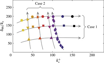
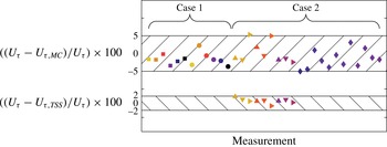
The two rough-wall Cases. The arrows show the direction of increasing Reynolds number for each Case. All symbols are defined in table 2.

2.3 Experiments
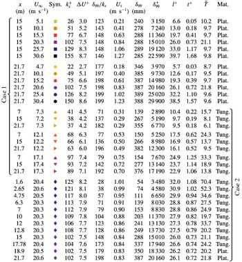
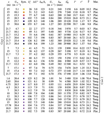
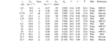
The rough-wall HWA measurements fall into two regimes: profiles taken over a range of free stream velocities, but at a fixed streamwise location (15 and 21.7 m) – hereafter referred to as Case 1 measurements – and profiles taken at a fixed streamwise velocity, but at varying distances from the trip – hereafter referred to as Case 2 measurements. All experimental conditions for Case 1 and Case 2 are summarised in table 2. While both the Case 1 and Case 2 data span a similar friction Reynolds number range, the evolution of the roughness Reynolds number,
 $k_{s}^{+}$
, differs greatly between the two types of development. This is demonstrated in figure 3. Case 1 developments span a range of
 $k_{s}^{+}$
values at approximately constant
 ${\it\delta}_{99}/k_{s}$
. Conversely, Case 2 data have approximately constant
 $k_{s}^{+}$
with increasing
 ${\it\delta}_{99}^{+}$
, but cover a range of
 ${\it\delta}_{99}/k_{s}$
. The arrows in figure 3 show the direction of increasing
 ${\it\delta}_{99}^{+}$
for each Case. Note that all rough-wall data in table 2 are coloured according to their
 $k_{s}^{+}$
value; light data points indicate a low
 $k_{s}^{+}$
, while dark data points indicate a high
 $k_{s}^{+}$
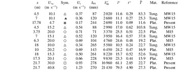
. A similar summary of the smooth-wall measurements is provided in table 3. Across all measurements, data denoted by triangular symbols were obtained using a multi-wire HWA probe, with all other data gathered using single-wire HWA probes. The multi-wire HWA measurements employ a probe arrangement similar to that of Foss & Haw (Reference Foss and Haw1990), but the present probe occupies approximately 10 % of their probe’s volume. The arrangement has four wires and is capable of measuring streamwise and wall-normal velocity fluctuations, and spanwise vorticity fluctuations. In the present study, only one wall-parallel wire on the multi-wire probe was employed to obtain streamwise velocities. For identification purposes, however, these data are denoted ‘multi-wire’ data, whereas those obtained using a single-wire probe are referred to as ‘single-wire’ data.
Details of the rough-wall experimental data.
 ${\it\delta}_{99}$
is the wall-normal location at which the mean streamwise velocity is 99 % of
 $U_{\infty }$
.
 $\tilde{T}=TU_{\infty }/{\it\delta}_{99}\times 10^{-3}$
and Plat. and Tung. are abbreviations for Platinum and Platinum-coated Tungsten, respectively.
Details of the smooth-wall experimental data. The abbreviations MW15 and M15 refer to Morrill-Winter et al. (Reference Morrill-Winter, Klewicki, Baidya and Marusic2015) and Marusic et al. (Reference Marusic, Chauhan, Kulandaivelu and Hutchins2015), respectively. Other abbreviations and units are as given in table 2.
Details of the multi-wire probe geometry, operating conditions and calibration procedure are provided in Morrill-Winter et al. (Reference Morrill-Winter, Klewicki, Baidya and Marusic2015). All single-wire rough-wall data were obtained using probes that were operated in constant temperature mode using a Melbourne University Constant Temperature Anemometer (MUCTA II) of in-house design. The overheat ratio was chosen to maintain the probe temperature at approximately
 $200\,^{\circ }\text{C}$
above ambient temperature. The lowest frequency response of the system to an external square wave was approximately 18 kHz, occurring at zero free stream velocity. The single element probes were constructed using Dantec 55P15 boundary layer type prongs with a tip spacing of 1.5 mm. Wollaston or copper-coated platinum-coated tungsten wires were soldered to the prong tips and etched to expose a
 $2.5~{\rm\mu}\text{m}$
diameter platinum or platinum-coated tungsten filament of length,
 $l=0.5~\text{mm}$
. The hot-wire signals were filtered using a low-pass analogue filter (Frequency Devices 9002), and were sampled using a Data Translation DT9836 Series true 16 bit data-acquisition board. Details of the sampling frequencies and filter settings for each rough-wall measurement are presented in table 2.
The smooth-wall measurements of Marusic et al. (Reference Marusic, Chauhan, Kulandaivelu and Hutchins2015) employed
 $2.5~{\rm\mu}\text{m}$
diameter platinum filaments. For the three present smooth-wall datasets,
 $5~{\rm\mu}\text{m}$
diameter filaments with
 $l=1~\text{mm}$
were operated under the same conditions as the rough-wall single-wire HWA measurements described above. All single-wire hot wires were calibrated before and after each boundary layer traverse, and the atmospheric conditions were monitored throughout. Additionally, the intermediate single point recalibration technique was used to account for calibration drift during all measurements (Talluru et al.
Reference Talluru, Kulandaivelu, Hutchins and Marusic2014). A stationary Pitot-static tube pair located in the free stream constituted the calibration standard for all single-wire measurements. A third-order polynomial fit to the calibration data was used to convert the hot-wire voltages to velocities.
The location of the probe relative to the smooth wall was determined using a wall-normal traversing microscope. The microscope was equipped with a digital micrometer (CDI BG3600) with a resolution of
 $1~{\rm\mu}\text{m}$
. The distance between the probe and the wall was determined as the wall-normal distance between the location at which the probe was in focus and the location at which the wall was in focus. Repeatability tests suggest that the maximum wall-normal error inherent to this process is
 $\pm 25~{\rm\mu}\text{m}$
. For the rough-wall measurements, the same procedure was not possible due to the local heterogeneity of the sandpaper. Instead, a 250 mm
 $\times$
250 mm aluminium tooling plate was placed on the surface of the roughness. The location of the probe relative to the top surface of the plate was determined using the procedure described above. The plate was subsequently removed and the probe was moved towards the wall by a distance equal to the thickness of the plate (9.52 mm
 $\pm$
0.02 mm). Thus, the wall-normal location of the probe above the rough wall was determined relative to the plane defined by the local roughness peaks (that is,
 $z=0$
is located at the roughness crest).
For the drag balance measurements, the friction force on the floating element was registered by a load cell and digitally sampled. Data were acquired across the full range of free stream velocities explored herein. The load cell was calibrated against free-hanging weights of accurately known mass before and after each measurement, and a linear curve was fitted to the calibration data. As is demonstrated by Baars et al. (Reference Baars, Squire, Talluru, Abbassi, Hutchins and Marusic2016), the variation in the wall drag across the floating element is approximately linear, meaning that the integrated drag across the element is equal to the local value at the centre of the element to within 0.024 %. The estimated experimental uncertainty of the drag balance measurements is
 $\pm 2.3\,\%$
at
 $U_{\infty }\approx 5~\text{m}~\text{s}^{-1}$
, with less error at higher
 $U_{\infty }$
. The present rough-wall profiles obtained above the drag balance were taken at 21.7 m rather than at the streamwise centre of the drag balance, introducing an additional error at
 $U_{\infty }\approx 5~\text{m}~\text{s}^{-1}$
of 0.2 % (again, with less error at higher
 $U_{\infty }$
). Further details of the drag balance and its operation are given in Baars et al. (Reference Baars, Squire, Talluru, Abbassi, Hutchins and Marusic2016).
2.4 Friction velocity
The results from the drag balance measurements only directly apply to the rough-wall data taken at
 $x=21.7~\text{m}$
. For the remaining data, an alternative approach is required. One popular method to determine
 $U_{{\it\tau}}$
is to equate the total stress – viscous stress and Reynolds shear stress – and wall shear stress in the inner part of the boundary layer. However, this approach demands an accurate measure of a velocity cross-correlation,
 $\overline{uw}$
, and a mean velocity gradient,
 $\partial U/\partial z$
. Aside from the fact that the former is not obtained for the majority of the measurements presented here (which employ only a single wire), both statistics are difficult to accurately obtain empirically. It is therefore common in both smooth- and rough-wall flows, to find
 $U_{{\it\tau}}$
indirectly using some variation of the Clauser (Reference Clauser1956) approach. This involves forcing the mean velocity to adhere to a predefined logarithmic law. A caveat of this method is that it requires knowledge of the region over which the logarithmic law is valid (classically, synonymous with an inertial sublayer).
Wei et al. (Reference Wei, Fife, Klewicki and McMurtry2005) formally define the start of the inertial region,
 $z_{I}$
, by quantifying the wall-normal location at which the viscous force loses dominant order. By examining the balance of the terms in the mean momentum equation across the smooth-wall boundary layer, Wei et al. (Reference Wei, Fife, Klewicki and McMurtry2005) show
 $z_{I}^{+}$
occurs just exterior to the peak in the Reynolds shear stress,
 $z_{m}^{+}$
(the zero crossing in the Reynolds shear stress gradient). It is well documented that above smooth walls the Reynolds shear stress attains a maximum at
 $z_{m}^{+}\approx 1.9\sqrt{{\it\delta}^{+}}$
(Afzal Reference Afzal1982; Sreenivasan & Sahay Reference Sreenivasan and Sahay1997; Wei et al.
Reference Wei, Fife, Klewicki and McMurtry2005). Thus, (Wei et al.
Reference Wei, Fife, Klewicki and McMurtry2005) provide analytical evidence that in smooth-wall flows
 $z_{I}^{+}$
scales with
 $\sqrt{{\it\delta}^{+}}$
. Empirical evidence for this scaling is provided by Marusic et al. (Reference Marusic, Monty, Hultmark and Smits2013), who demonstrate across a range of high Reynolds number smooth-wall facilities that log-linearity is observed as the leading-order function in both the streamwise mean velocity and turbulence intensity when the beginning of the logarithmic region is chosen to scale with
 $\sqrt{{\it\delta}^{+}}$
(note that log-linearity of the streamwise turbulence intensity on the inertial subrange is predicted by the attached eddy hypothesis of Townsend (Reference Townsend1976)). Therefore, in the present study the smooth-wall friction velocity is determined using a Clauser (Reference Clauser1956) fit approach with
 ${\it\kappa}=0.39$
and
 $A=4.3$
across the inertial region limits employed by Marusic et al. (Reference Marusic, Monty, Hultmark and Smits2013). However, Marusic et al. (Reference Marusic, Monty, Hultmark and Smits2013) use the composite fit of Chauhan, Monkewitz & Nagib (Reference Chauhan, Monkewitz and Nagib2009) to determine the boundary layer thickness, whereas here
 ${\it\delta}_{99}$
is defined as the wall-normal location at which the mean streamwise velocity is 99 % of its free stream value. The ratio between these two definitions of the boundary layer thickness has only a weak trend with friction Reynolds number; i.e.
 $Re_{{\it\tau}}\approx 1.26\times {\it\delta}_{99}^{+}$
, where
 $Re_{{\it\tau}}$
is computed using composite value, and
 ${\it\delta}_{99}^{+}$
uses the present definition. Thus, the inner and outer bounds of the inertial region used by Marusic et al. (Reference Marusic, Monty, Hultmark and Smits2013) are adapted here from
 $z_{I}^{+}=3\sqrt{Re_{{\it\tau}}}$
and
 $z^{+}/Re_{{\it\tau}}=0.15$
, to
 $z_{I}^{+}=3.4\sqrt{{\it\delta}_{99}^{+}}$
and
 $z^{+}/{\it\delta}_{99}^{+}=0.19$
, respectively.
As emphasized by Perry & Joubert (Reference Perry and Joubert1963), there are two additional unknowns in the rough-wall formulation of the logarithmic law, namely
 ${\it\epsilon}$
and
 ${\rm\Delta}U$
(see (2.1)). The wall correction parameter,
 ${\it\epsilon}$
, accounts for the fact that the roughness itself displaces the entire flow away from the wall. It is therefore dependent on both the flow and the roughness. Thom (Reference Thom1971) found experimentally, and Jackson (Reference Jackson1981) provided theoretical arguments, that the difference between the roughness height and
 ${\it\epsilon}$
(for them
 $z=0$
is located at the roughness trough) physically represents the mean height of momentum absorption by the surface. Thus, to correctly measure
 ${\it\epsilon}$
the centroid of the drag profile in the roughness must be calculated; an exercise which is relatively straightforward when the nature of the flow within the roughness canopy is known (either via empirical observation – see Jackson (Reference Jackson1981) – or via numerical simulation – see Chan et al. (Reference Chan, MacDonald, Chung, Hutchins and Ooi2015)) but is currently impractical for complex roughnesses. In the rough-wall literature, it is common to employ the modified Clauser technique of Perry & Li (Reference Perry and Li1990) which chooses
 ${\it\epsilon}$
to maximise the extent of the logarithmic region of the mean streamwise velocity profile. Such an approach is only appropriate when there exists no data interior to the onset of the inertial region. However, there are few studies that examine where inertial dynamics begin to dominate rough-wall flows. The present study focusses primarily on outer-region rough-wall flow physics with large
 ${\it\delta}_{99}/k_{s}$
. Thus, the definition of
 ${\it\epsilon}$
employed here has negligible effect on the results, as long as the physical constraint that
 $0<{\it\epsilon}<k$
is satisfied (Raupach et al.
Reference Raupach, Antonia and Rajagopalan1991). For simplicity,
 ${\it\epsilon}=k/2$
is used here. However, it is noted that this definition has no physical justification.
In rough-wall flows, a prevalent assumption is that the flow is inertial starting from the tops of the roughness crests (for example Perry & Joubert (Reference Perry and Joubert1963), Perry & Li (Reference Perry and Li1990) and Schultz & Flack (Reference Schultz and Flack2003)). As noted by Mehdi, Klewicki & White (Reference Mehdi, Klewicki and White2013), this implies that the positive contribution of the Reynolds shear stress gradient (the integral of which across the boundary layer is equal to zero) to the mean momentum equation is confined to the roughness canopy regardless of friction Reynolds number. Mehdi et al. (Reference Mehdi, Klewicki and White2013) examined the balance of terms in the mean momentum equation for a series of experiments, and concluded that a similar structure existed for both smooth and rough walls, where for the rough-wall flows the ratio of scales of
 ${\it\nu}/U_{{\it\tau}}$
,
 ${\it\delta}$
and
 $k$
influenced the wall-normal location at which inertial dynamics begin to dominate. Based on this, Mehdi et al. (Reference Mehdi, Klewicki and White2013) proposed
 $z_{m}^{+}$
as a surrogate scale for the onset of the inertial layer, where, since the transition to inertial mean dynamics is qualitatively the same as for smooth walls,
 $z_{I}^{+}=C_{I}z_{m}^{+}$
. The constant
 $C_{I}$
is
 $O(1)$
, and
 $z_{m}^{+}$
depends on the three length scales present in rough-wall flows:
 $$\begin{eqnarray}\displaystyle z_{m}=C({\it\nu}/U_{{\it\tau}})^{a}k_{s}^{b}{\it\delta}^{c}. & & \displaystyle\end{eqnarray}$$
For the data examined by Mehdi et al. (Reference Mehdi, Klewicki and White2013), three regimes are identified. These correspond to the ratio of
 $k_{s}$
to
 $z_{m}$
being less than, equal to or greater than
 $O(1)$
, with the constants
 $C$
,
 $a$
,
 $b$
and
 $c$
empirically estimated for each regime. Visual inspection across all of the present rough-wall data reveals that the wall-normal location of the beginning of logarithmic decay in the streamwise turbulence intensity profiles is always significantly exterior to
 $k_{s}$
. That is,
 $z_{m}/k_{s}>O(1)$
, so the constants
 $C$
,
 $a$
,
 $b$
and
 $c$
recommended by Mehdi et al. (Reference Mehdi, Klewicki and White2013) in this regime are employed in this paper:
 $$\begin{eqnarray}\displaystyle z_{I}=2.5\times 0.89({\it\nu}/U_{{\it\tau}})^{0.36}k_{s}^{0}{\it\delta}_{99}^{0.64}. & & \displaystyle\end{eqnarray}$$
Here
 $C_{I}=2.5$
is assumed, and justification of this value is provided in § 3.3. Note that
 $C$
,
 $a$
,
 $b$
and
 $c$
in (2.4) were obtained by Mehdi et al. (Reference Mehdi, Klewicki and White2013) by fitting (2.3) to only a few rough-wall datapoints. Further investigation of these constants is required using more data that span a wider range of boundary layer parameters (all with
 $z_{m}/k_{s}>O(1)$
). As for the outer location of the rough-wall inertial sublayer, this is relatively inconsequential in the present study and is taken, as for the smooth wall, to be
 $z^{+}=0.19{\it\delta}_{99}^{+}$
(recall that
 $0.19{\it\delta}_{99}\approx 0.15{\it\delta}_{c}$
, where
 ${\it\delta}_{c}$
is computed using the composite fit of Chauhan et al. (Reference Chauhan, Monkewitz and Nagib2009)).
For the rough-wall data above the drag balance (Case 1 at 21.7 m),
 $U_{{\it\tau}}$
is determined from a linear fit of the form
 $U_{{\it\tau}}/{\it\nu}=C_{1}U_{\infty }/{\it\nu}+C_{2}$
applied to the drag balance data. To determine
 $U_{{\it\tau}}$
for the remaining rough-wall data, the characteristic relationship between roughness function and equivalent sand grain roughness (see figure 2) is employed. This relationship is determined using only data taken above the drag balance, for which
 $U_{{\it\tau}}$
can be determined directly. Here, a spline fit to a cubic interpolation of these data (shown by the solid line in figure 2) characterises the dependence of
 ${\rm\Delta}U^{+}$
on
 $k_{s}^{+}$
. The relationship is assumed to be a property of the roughness and is hence taken to be applicable for all of the present rough-wall measurements. The wall friction velocities of the remaining rough-wall data are then determined by forcing these data to lie on the fitted curve, and minimizing the least-squares error between the inner-normalised streamwise velocity profile and the rough-wall logarithmic law (2.1) across the inertial sublayer using
 ${\it\kappa}=0.39$
and
 $A=4.3$
. Note that using
 ${\it\epsilon}=0$
mm and
 ${\it\epsilon}=k$
causes the determined
 $U_{{\it\tau}}$
to change by at most
 $-$
2.0 % and 2.2 %, respectively, across all rough-wall profiles. However,
 ${\it\epsilon}$
has the most affect when
 $x$
is small, where the boundary layer is thinnest. Downstream of
 $x=4.75~\text{m}$
,
 $U_{{\it\tau}}$
changes by less than 0.8 % when
 ${\it\epsilon}=0~\text{mm}$
or
 ${\it\epsilon}=k~\text{mm}$
.
3 Results
3.1 Inner-normalised turbulence statistics
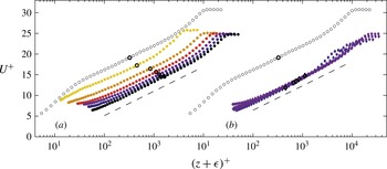
Figure 4 shows the inner-normalised mean streamwise velocity profiles above the rough wall. Figure 4(a) presents Case 1 profiles at 21.7 m (for which
 $U_{{\it\tau}}$
is determined directly from the drag balance data), while figure 4(b) shows single-wire Case 2 data at
 $U_{\infty }\approx 20~\text{m}~\text{s}^{-1}$
. In both plots, smooth-wall data at
 ${\it\delta}_{99}^{+}=9830$
are included for comparison, and the location of
 $z_{I}$
(calculated using (2.4)) for a particular profile is indicated by the symbol with a thick black outline. The latter is true for all remaining figures in this paper. Recall that the Case 1 data are taken at approximately matched
 ${\it\delta}_{99}/k_{s}$
, with
 $k_{s}^{+}$
ranging from the transitionally rough (
 $k_{s}^{+}=22$
) to fully rough regime (
 $k_{s}^{+}=150$
) with increasing Reynolds number. Conversely, all Case 2 data are at approximately matched
 $k_{s}^{+}$
, but
 ${\it\delta}_{99}/k_{s}$
ranges with streamwise development from relatively small (
 ${\it\delta}_{99}/k_{s}=28$
) to very large (
 ${\it\delta}_{99}/k_{s}=198$
).
Comparison of streamwise mean velocity between the smooth and rough walls. (a) Shows the rough-wall data for Case 1 at 21.7 m, (b) shows the single-wire rough-wall data for Case 2 at
 $U_{\infty }\approx 20~\text{m}~\text{s}^{-1}$
with the data at every second streamwise location removed for clarity. Smooth-wall data at
 ${\it\delta}_{99}^{+}=9830$
is included in both plots. The symbols with thick black outlines show the location of the onset of inertial dynamics according to (2.4). Dashed black lines have a slope of
 $1/{\it\kappa}=1/0.39$
.

The results in figure 4 show a convincing log-linear region for all profiles, with a slope very similar to the logarithmic slope of the smooth-wall data; the dashed lines in figure 4 show a log-linear slope of
 $1/{\it\kappa}$
. (Note that the approach used to determine
 $U_{{\it\tau}}$
for the data shown in figure 4(a) does not assume that there is a logarithmic profile in the mean streamwise velocity.) The results also show the well-known result that the rough wall causes a vertical shift,
 ${\rm\Delta}U^{+}$
, in the inner-normalised mean streamwise velocity due to the increase in drag above the rough wall (relative to a smooth wall) and the resulting increase in momentum flux towards the wall (Raupach et al.
Reference Raupach, Antonia and Rajagopalan1991). In smooth-wall flows the no-slip condition requires that at
 $z=0$
,
 $U=0$
, while for rough walls the effective location of the wall varies. Consequently, for the rough wall flows there is no constraint that
 $U=0$
at
 $z+{\it\epsilon}=0$
. Nonetheless, there is a location somewhere within the roughness canopy where
 $U=0$
. Thus, because of the downward shift in the rough-wall profiles (
 ${\rm\Delta}U^{+}$
), the near-wall characteristics of the mean streamwise velocity profile must differ between the smooth and rough walls. Due to this near-wall modification, most profiles in figure 4 for which
 $7\lesssim {\rm\Delta}U^{+}\lesssim 10$
appear to be approximately log-linear down to the lowest measured wall-normal position. Of course, these profiles may contain error near to the wall due to the choice of
 ${\it\epsilon}$
described in § 2.4. However, it seems that such behaviour should be observed at some
 ${\rm\Delta}U^{+}$
for any sensible choice of
 ${\it\epsilon}$
. Based upon its classically defined attributes, the logarithmic region is herein taken to coincide with the inertial sublayer. Approximate log-linearity of the mean streamwise velocity is thus not sufficient to define the inertial sublayer. That is, although the mean streamwise velocity may exhibit log-linearity external to the roughness crest, the wall-normal location of the beginning of the logarithmic region (or inertial sublayer) may be further out in the boundary layer. Such behaviour occurs in smooth-wall flow, where
 $U^{+}$
is approximately logarithmic interior to
 $z_{I}$
(see Marusic et al.
Reference Marusic, Monty, Hultmark and Smits2013).
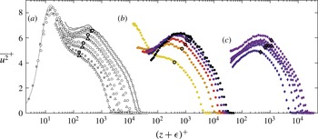
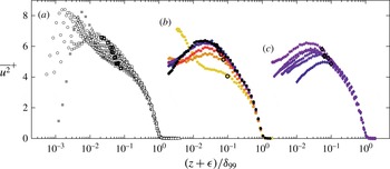
The friction Reynolds number trends of the streamwise velocity variance above the smooth and rough wall. In (a), the smooth-wall data are presented with some intermediate Reynolds number data removed for clarity. The thin grey line shows the boundary layer DNS of Sillero, Jiménez & Moser (Reference Sillero, Jiménez and Moser2013) and the thick grey lines show the two highest Reynolds number smooth-wall profiles, corrected for spatial attenuation using the approach introduced by Smits et al. (Reference Smits, Monty, Hultmark, Bailey, Hutchins and Marusic2011). (b) Shows the rough-wall data for Case 1 at 21.7 m, and (c) shows the single-wire rough-wall data for Case 2 at
 $U_{\infty }\approx 20~\text{m}~\text{s}^{-1}$
with every second streamwise location removed for clarity. The symbols with thick black outlines show the location of the onset of inertial dynamics according to (2.4).

The Reynolds number trends of the streamwise velocity variance are presented in figure 5. Smooth-wall data are shown in figure 5(a), Case 1 data at 21.7 m are shown in figure 5(b) and single-wire Case 2 data at
 $U_{\infty }\approx$
20 are presented in figure 5(c). All data show consistent development trends with increasing friction Reynolds number. However, the two highest Reynolds number smooth-wall profiles have significantly poorer spatial resolution (
 $l^{+}=$
61 and 80, respectively) than the other smooth-wall profiles (
 $l^{+}<$
26). Hutchins et al. (Reference Hutchins, Nickels, Marusic and Chong2009) show that in smooth-wall turbulent flows an increase in
 $l^{+}$
causes attenuation of the streamwise variance that is largest near to the wall, where the contributing scales of motion are relatively small. In this paper, the smooth-wall data are employed to make comparisons with rough-wall data in the outer region of the flow. Such comparisons can lead to specious interpretations when the effect of spatial resolution is not carefully considered. The thick grey lines in figure 5(a) show the two highest Reynolds number smooth-wall profiles, corrected for spatial attenuation affects using the approach of Smits et al. (Reference Smits, Monty, Hultmark, Bailey, Hutchins and Marusic2011). The corrected data indicate that for the smooth-wall data there is little effect on
 $\overline{u^{2}}^{+}$
due to spatial averaging external to
 $z\approx z_{I}$
(the region of interest in this paper). Although it has not been validated, it is prudent to assume that the correction proposed by Smits et al. (Reference Smits, Monty, Hultmark, Bailey, Hutchins and Marusic2011) provides a reasonable estimate of the effect of spatial attenuation in rough-wall flows, at least away from the near-wall region. It is therefore unlikely that any of the rough-wall
 $\overline{u^{2}}^{+}$
profiles presented herein (all with
 $l^{+}<40$
) are discernibly influenced by spatial attenuation beyond
 $(z+{\it\epsilon})\approx z_{I}$
.
Comparing figure 5(a–c), the smooth and fully rough variances exhibit very similar development trends with friction Reynolds number. In accord with Townsend’s (Reference Townsend1976) attached eddy hypothesis, both wall conditions appear to exhibit a region of log-linear slope (see § 3.3), that lengthens (in wall units) with increasing Reynolds number. At the lowest Reynolds number in figure 5(b), the rough wall appears to have little effect on the general shape of the streamwise variance profile, with a near-wall peak clearly visible at
 $z^{+}\approx 15$
. With increasing friction and roughness Reynolds numbers, the magnitude of the near-wall peak diminishes, such that at
 ${\it\delta}_{99}^{+}=29\,900$
and
 $k_{s}^{+}=150$
, no near-wall peak is apparent. Note however, that the spatial resolution varies substantially in figure 5(b): from
 $l^{+}=5.7$
at the lowest friction Reynolds number to
 $l^{+}=38.5$
at the highest. Therefore, spatial resolution effects are also partially responsible for the reduction in the near-wall peak intensity observed with increasing
 ${\it\delta}_{99}^{+}$
. However, these effects are not sufficient to account for the complete absence of a near-wall peak at
 ${\it\delta}_{99}^{+}=29\,900$
; Hutchins et al. (Reference Hutchins, Nickels, Marusic and Chong2009) suggest from their data that for
 $l^{+}<20$
the error in the inner-normalised streamwise variance due to spatial averaging should be less than
 $10\,\%$
for
 ${\it\delta}_{99}^{+}\gtrsim 3500$
. The lack of a near-wall variance peak is well documented in fully rough flows and is associated with a destruction/disturbance of the near-wall cycle in the immediate vicinity of the roughness elements (Grass Reference Grass1971; Schultz & Flack Reference Schultz and Flack2007). This disturbance of the near-wall cycle appears to be a gradual process with increasing
 $k_{s}^{+}$
and is likely tied to the corresponding increase in pressure drag at the wall. While a clear near-wall peak is observed in the transitionally rough data in figure 5(b), no such peak is observed in the fully rough data in figure 5(c), even at approximately matched friction Reynolds number. Interestingly, there appears to be little affect in changing
 ${\it\delta}_{99}/k_{s}$
(which varies from 28 to 198 in figure 5
c) on the general shape of the variance profiles. Note, however, that for the majority of the rough-wall data considered here, the height of the roughness relative to the boundary layer thickness would typically be considered small. This is especially true when compared to some pre-existing measurements in which outer-layer similarity was not observed. For example, Krogstadt & Antonia (Reference Krogstadt and Antonia1999) studied a case with
 $k_{s}/{\it\delta}_{99}=1/7$
, whereas the largest relative roughness presented here is
 $k_{s}/{\it\delta}_{99}=1/28$
. It is worth noting that such empirical studies are susceptable to errors in determining the virtual origin (that is, determining
 ${\it\epsilon}$
) that can influence the outer region.
3.2 Outer-normalised turbulence statistics
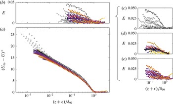
(a) The velocity defect
 $(U_{\infty }-U)/U_{{\it\tau}}$
for all smooth- and rough-wall data. The deviation
 $E$
about the mean defect
 $\overline{D}^{+}$
as defined in (3.1) is presented for all of the data in (b), and for the smooth wall, rough-wall Case 1 and rough-wall Case 2 data in (c–e), respectively.

Figure 6 compares the smooth- and rough-wall mean velocity profiles in defect form. Examination of such plots is a common approach for assessing the validity of Townsend’s (Reference Townsend1956) wall-similarity hypothesis. If the hypothesis is correct, high Reynolds number data normalised in this way should define a single profile in the outer region regardless of the wall condition. Figure 6(a) shows that, with the exception of a few low Reynolds number smooth-wall profiles, the velocity defect data (smooth and rough wall) follow a single outer-layer profile. To probe these results in greater detail, the deviation of the individual profiles from a mean defect profile is calculated. This is presented in figure 6(c–e) where the deviation,
 $E$
, is plotted for the smooth-wall data, and Case 1 and Case 2 rough-wall data, respectively. Here,
 $$\begin{eqnarray}\displaystyle E=\left|\frac{(U_{\infty }-U)^{+}-\overline{D}^{+}}{U^{+}-{\rm\Delta}U^{+}}\right|, & & \displaystyle\end{eqnarray}$$
where
 $\overline{D}^{+}$
is the mean defect of all of the smooth- and rough-wall profiles. It can be seen that the maximum deviation observed in any of the profiles in the outer layer is
 ${<}5\,\%$
. Numerous studies have reported an increase in the wake strength,
 ${\it\Pi}$
, of rough-wall flows relative to that for smooth-wall flows (Krogstad et al.
Reference Krogstad, Antonia and Browne1992; Keirsbulck et al.
Reference Keirsbulck, Labraga, Mazouz and Tournier2002; Akinlade et al.
Reference Akinlade, Bergstrom, Tachie and Castillo2004; Bergstrom, Akinlade & Tachie Reference Bergstrom, Akinlade and Tachie2005; Castro Reference Castro2007). Castro, Segalini & Alfredsson (Reference Castro, Segalini and Alfredsson2013) suggests that
 ${\it\Pi}$
may be a particularly sensitive measure of whether the outer-region boundary layer structure is truly universal, noting rough-wall studies in which the outer-layer stress profiles collapse well with those for smooth walls, but where
 ${\it\Pi}$
differs. Based on an examination of extant rough-wall data, Castro et al. (Reference Castro, Segalini and Alfredsson2013) suggest that to ensure outer flow similarity the flow must be fully rough with
 ${\it\delta}_{99}/k_{s}\gtrsim 11$
(note Castro et al. (Reference Castro, Segalini and Alfredsson2013) actually pose their approximate criterion on
 ${\it\delta}_{99}/z_{0}$
, where
 $z_{0}$
is an alternative measure to
 $k_{s}^{+}$
: using
 ${\it\kappa}=0.39$
,
 $k_{s}=27.5z_{0}$
). In figure 6(a) all data satisfy
 ${\it\delta}_{99}/k_{s}\gtrsim 11$
. Evidence of invariance, however, is observed even for data that are transitionally rough.
It is important to note that perfect invariance of the mean defect velocity is not expected even for smooth-wall flows. For example, numerous studies (Erm & Joubert Reference Erm and Joubert1991; Schlatter & Örlü Reference Schlatter and Örlü2012; Marusic et al.
Reference Marusic, Chauhan, Kulandaivelu and Hutchins2015) have shown that
 ${\it\Pi}$
can be a strong function of
 $x$
immediately downstream of the trip, with the tripping strength also having an effect. Only at some distance downstream of the trip does
 ${\it\Pi}$
appear to become asymptotically constant (see Marusic et al.
Reference Marusic, Chauhan, Kulandaivelu and Hutchins2015). There are also questions regarding whether
 ${\it\Pi}$
depends on Reynolds number (Coles Reference Coles1962; De Graaff & Eaton Reference De Graaff and Eaton2000; Perry, Marusic & Jones Reference Perry, Marusic and Jones2002). Therefore, the observed agreement between the smooth- and rough-wall defect data provides only ostensible support for Townsend’s wall-similarity hypothesis. Certainly, the deviation
 $E$
is generally higher for the smooth-wall data (figure 6
c) than for the rough-wall data, particularly at lower speeds. This may be indicative of some dependence on upstream conditions. It is, however, encouraging that the profiles of
 $E$
are very similar between the smooth and rough walls; suggesting that Townsend’s hypothesis is, at worst, a good approximation for the mean streamwise velocity defect.
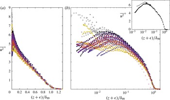
The streamwise velocity variance for all smooth- and rough-wall data. A linear abscissa is used in (a) and a logarithmic abscissa is used in (b). In the inset of (b), the highest Reynolds number smooth-wall profile (
 ${\it\delta}_{99}^{+}=21\,430$
) is compared to the highest Reynolds number rough-wall profile (
 ${\it\delta}_{99}^{+}=29\,900$
).

In figure 7 all smooth- and rough-wall turbulence intensity profiles are presented on an outer-normalised abscissa (linearly and logarithmically spaced in figure 7(a,b), respectively). All rough- and smooth-wall data apparently merge beyond
 $(z+{\it\epsilon})/{\it\delta}_{99}\approx 0.5$
. However, even at this location the data spreads over a range,
 $\overline{u^{2}}_{max}^{+}-\overline{u^{2}}_{min}^{+}\approx 0.7$
. In figure 7(c) the highest Reynolds number smooth- and rough-wall data are compared. Here, excellent agreement between these two profiles is observed external to the beginning of the inertial sublayer, providing convincing support for Townsend’s hypothesis, at least for fully rough flows at high friction Reynolds numbers. Comparisons of smooth- and rough-wall streamwise variance profiles across a wide range of friction and roughness Reynolds numbers (such as in figure 7
b) are common in the literature for assessing the efficacy of Townsend’s hypothesis. However, such comparisons can be difficult to interpret since the variance has a strong dependence on
 ${\it\delta}_{99}^{+}$
. See, for example, figure 8(a) where all inner-normalised smooth-wall variance profiles are plotted on an outer-normalised abscissa. Disregarding any experimental error in the data, and acknowledging that any effects of poor spatial resolution are negligible beyond
 $z/{\it\delta}_{99}\approx 0.02$
(see § 3.1), the spread of the profiles internal to
 $z/{\it\delta}_{99}\approx 0.2$
in figure 8(a) is evidently due to the inherent trends with
 ${\it\delta}_{99}^{+}$
. Returning to figure 7, it appears that data with
 $k_{s}^{+}\lesssim 70$
(lighter shaded symbols) are attenuated below the fully rough and smooth-wall data. Additionally, the degree of attenuation apparently depends on the magnitude of
 $k_{s}^{+}$
; with increasing
 $k_{s}^{+}$
(darkening symbols) the transitionally rough data lie increasingly closer to the cluster of fully rough and smooth profiles. However, for the present experiments, data with a low
 $k_{s}^{+}$
typically also have a low
 ${\it\delta}_{99}^{+}$
. Therefore, in figure 7 it is difficult to isolate trends with
 $k_{s}^{+}$
from trends with
 ${\it\delta}_{99}^{+}$
. Note that comparison of rough-wall variance profiles at matched friction Reynolds number but different roughness Reynolds number (such as the lowest friction Reynolds number profiles in figure 8(b,c), respectively) suggest that the trends described above are related to
 $k_{s}^{+}$
, rather than
 ${\it\delta}_{99}^{+}$
. This is discussed in further detail in §§ 3.3 and 3.4.
The friction Reynolds number trends of the streamwise velocity variance above the smooth and rough wall. (a) Shows the smooth-wall data with some intermediate Reynolds number data removed for clarity, (b) shows the rough-wall data for Case 1 at 21.7 m, (c) shows the single-wire rough-wall data for Case 2 at
 $U_{\infty }\approx 20~\text{m}~\text{s}^{-1}$
with every second streamwise location removed for clarity. The symbols with thick black outlines show the location of the onset of inertial dynamics according to (2.4).

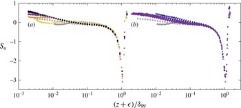
Streamwise skewness profiles for the smooth and rough walls. (a) Shows the rough-wall data for Case 1 at 21.7 m, (b) shows the single-wire rough-wall data for Case 2 at
 $U_{\infty }\approx 20~\text{m}~\text{s}^{-1}$
. The highest and lowest Reynolds number smooth-wall profiles are included in each plot for comparison. Note that data beyond
 $(z+{\it\epsilon})/{\it\delta}_{99}=1.5$
are removed for clarity.

The streamwise velocity skewness profiles for the Case 1 data at 21.7 m and single-wire Case 2 data at
 $U_{\infty }\approx 20~\text{m}~\text{s}^{-1}$
are presented in figure 9(a,b), respectively. For comparison, the highest and lowest friction Reynolds number smooth-wall skewness profiles are also included in both figures. Note that the skewness is normalised by the standard deviation cubed and is therefore not subject to errors in
 $U_{{\it\tau}}$
. Interestingly, the smooth- and rough-wall Case 1 data in figure 9(a) apparently merge beyond
 $(z+{\it\epsilon})/{\it\delta}_{99}\approx 0.02$
, suggesting that
 $k_{s}^{+}$
has little effect on skewness. Conversely, in figure 7(b) there is a clear trend in the rough-wall data. Inside of
 $(z+{\it\epsilon})/{\it\delta}_{99}\approx 0.2$
the rough-wall skewness is larger than that of the smooth wall, with a greater difference nearer to the wall. The discrepancy between the smooth- and rough-wall data in this region also appears to decrease with increasing distance from the trip,
 $x$
(that is, increasing
 ${\it\delta}_{99}^{+}$
or increasing
 ${\it\delta}_{99}/k_{s}$
). Since the range of Reynolds numbers spanned in figure 9(a,b) is approximately the same, it appears that the rough-wall skewness trends observed in figure 9(b) result from the changes in
 ${\it\delta}_{99}/k_{s}$
rather than the changes in
 ${\it\delta}_{99}^{+}$
. However, this result is opposite to that observed in figures 5 and 8. Here, changing
 $k_{s}^{+}$
appeared to influence the general shape of the streamwise velocity variance, whereas changing
 ${\it\delta}_{99}/k_{s}$
had seemingly little influence (at least over the range of values considered).
3.3 The inertial sublayer in rough-wall flows
In wall-bounded flows, there is now considerable support for the existence of a logarithmic region (or inertial sublayer in physical space). Here, the streamwise velocity is independent of first-order viscous effects and scales with
 $U_{{\it\tau}}$
regardless of the characteristic length scale for
 $z$
(an alternative viewpoint is that
 $z$
is the characteristic length scale). In smooth-wall flows, there is theoretical and experimental evidence that the wall-normal location of the beginning of the inertial sublayer scales with
 $\sqrt{{\it\delta}^{+}}$
, the geometric mean of the inner and outer length scales of the flow (Klewicki, Fife & Wei Reference Klewicki, Fife and Wei2009; Chin et al.
Reference Chin, Philip, Klewicki, Ooi and Marusic2014). In rough-wall flows, Mehdi et al. (Reference Mehdi, Klewicki and White2013) hypothesise and show evidence that, as in smooth-wall flows, the location of the onset of inertial dynamics scales with a geometric ratio of the scales present in the flow, including the length scales imposed by the roughness (see (2.3)).
In what is commonly referred to as the attached eddy hypothesis, Townsend (Reference Townsend1976) theorized that the logarithmic scaling of the wall can be associated with a three-dimensional distribution of self-similar eddying motions whose sizes scale with their distance from the wall. The attached eddy hypothesis is independent of viscosity and consistent with the leading-order mean dynamics in the boundary layer inertial sublayer. Townsend showed that this description leads to logarithmic profiles in the streamwise mean velocities, and in the spanwise and streamwise velocity variances. The latter is shown to have the form:
 $$\begin{eqnarray}\displaystyle \overline{u^{2}}^{+}=B_{1}-A_{1}\log \left(\frac{z+{\it\epsilon}}{{\it\delta}_{99}}\right). & & \displaystyle\end{eqnarray}$$
Note that the constant
 $A_{1}$
is expected to be universal, but
 $B_{1}$
is expected to change with external flow geometry. Marusic et al. (Reference Marusic, Monty, Hultmark and Smits2013) provide empirical evidence for (3.2) in smooth-wall flows over approximately the same wall-normal domain as the logarithmic region of the mean velocity profile.
In figure 10 the streamwise mean velocity and turbulence intensity are presented for all rough-wall profiles. On the abscissa, the wall-normal location,
 $z$
, is normalised by the predicted location of the onset of inertial dynamics,
 $z_{I}$
, aligning
 $(z+{\it\epsilon})=z_{I}$
for each profile at
 $(z+{\it\epsilon})/z_{I}=1$
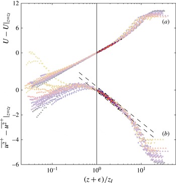
. For clarity, the streamwise mean velocities and turbulence intensities in figure 10 are shifted by their respective values at the location of the beginning of the inertial sublayer. Using (3.2), it is easy to show
 $$\begin{eqnarray}\displaystyle \overline{u^{2}}^{+}-\overline{u^{2}}^{+}|_{(z+{\it\epsilon})=z_{I}}=A_{1}\log \left(\frac{z+{\it\epsilon}}{z_{I}}\right). & & \displaystyle\end{eqnarray}$$
That is, figure 10 is independent of the constant
 $B_{1}$
across the inertial sublayer. The darker points in each profile indicate the region of data contained within the inertial sublayer (defined here for rough-wall flows as
 $z_{I}^{+}<z^{+}<0.19{\it\delta}_{99}^{+}$
). The data all show a distinct logarithmic profile in both the streamwise mean velocity and turbulence intensity, with uniformly good agreement across the full range of Reynolds numbers and roughness conditions. A similar observation was also made by Hultmark et al. (Reference Hultmark, Vallikivi, Bailey and Smits2013) in high Reynolds number rough-wall pipe flows, but using a different normalisation for
 $z$
. The dashed black lines that bound the data in figure 10(b) have a slope of
 $A=1.26$
(Marusic et al.
Reference Marusic, Monty, Hultmark and Smits2013) and show a range in
 $\overline{u^{2}}^{+}-\overline{u^{2}}^{+}|_{z=z_{I}}$
of
 $\pm 0.2$
. Note that in order to obtain
 $z_{I}$
from the formulation of Mehdi et al. (Reference Mehdi, Klewicki and White2013) a value for the constant,
 $C_{I}$
, is required. Here,
 $C_{I}=2.5$
is used, since this yields good collapse of the data in figure 10. This paper, however, is not concerned with determining an exact value for
 $C_{I}$
. The important result here is that good collapse can be obtained using a fixed value for
 $C_{I}$
that is
 $O(1)$
.
The streamwise mean velocity and turbulence intensity with the abscissa shifted by the estimated location of the onset of inertial dynamics
 $z_{I}$
, and the ordinate shifted by its respective value at this location. All rough-wall data are presented. The dark points in each profile show the data contained within the inertial sublayer according to the definitions in § 2.4. The dashed black lines that bound the data in 10(b) have a slope of
 $A=1.26$
(Marusic et al.
Reference Marusic, Monty, Hultmark and Smits2013) and show a range
 $\overline{u^{2}}^{+}-\overline{u^{2}}^{+}|_{z=z_{I}}=\pm 0.2$
.

The results in figure 10 suggest that the formulation proposed by Mehdi et al. (Reference Mehdi, Klewicki and White2013) provides, for the current rough surface conditions (
 $z_{m}>k_{s}^{+}$
), a good estimate of the wall-normal scale at which inertial dynamics become dominant. Additionally, the slope of the logarithmic regions of the rough-wall streamwise mean velocities and turbulence intensities agree within experimental uncertainty to those found above smooth walls (Marusic et al.
Reference Marusic, Monty, Hultmark and Smits2013). This suggests similarity between the inertial region dynamics in smooth- and rough-wall flows. The poor collapse of the wake region of the streamwise velocity variance in figure 10 is, to some extent, due to the inherent friction Reynolds number trends associated with this statistic. However, figures 7 and 8 indicate that the outer region of the flow also has a dependence on
 $k_{s}^{+}$
at least for transitionally rough surfaces at low
 ${\it\delta}_{99}^{+}$
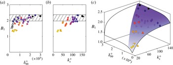
. In figure 11, the constant
 $B_{1}$
from (3.2) is presented as a function of friction and roughness Reynolds number. For each profile,
 $B_{1}$
is determined by minimizing the root-mean-square error between that profile and (3.2) across the inertial region with
 $A_{1}=1.26$
. For the smooth-wall data,
 $B_{1}$
appears to become approximately constant for
 ${\it\delta}_{99}^{+}\gtrsim 4000$
. The hatched regions in figure 11(a,b) show
 $B_{1}=2.17\pm 0.2$
, where
 $B_{1}=2.17$
was determined for the highest Reynolds number smooth-wall dataset and the range was chosen to match that shown by the dashed lines in figure 10(b). That is, for any two datasets with
 $B_{1}$
values that agree to within
 $0.4$
,
 $\overline{u^{2}}^{+}$
(when plotted against
 $(z+{\it\epsilon})/{\it\delta}_{99}$
) will exhibit equivalent collapse across the entire inertial sublayer to that observed in figure 10(b). For the rough-wall data,
 $B_{1}$
appears to be a weak function of
 ${\it\delta}_{99}^{+}$
and a strong function of
 $k_{s}^{+}$
; the purple surface in figure 11(c) shows the general trend of the data. At high
 $k_{s}^{+}$
and
 ${\it\delta}_{99}^{+}$
,
 $B_{1}$
appears to plateau to the same approximate value as for the smooth wall. For all flows with
 $B_{1}\simeq 2.17$
, similarity of the inner-normalised streamwise variance is observed beyond
 $z_{I}$
regardless of wall condition (accepting, of course, that there is universality in the wake region: see figure 7). Inertial and outer-layer collapse of the inner-normalised streamwise velocity variance is ostensibly observed for the present roughness geometry for
 ${\it\delta}_{99}^{+}\gtrsim 14\,000$
, or independent of
 ${\it\delta}_{99}^{+}$
if
 $k_{s}^{+}\gtrsim 100$
. At low/intermediate friction and roughness Reynolds numbers, however, it appears that for the present roughness
 $U_{{\it\tau}}$
and
 ${\it\delta}$
are not sufficient to scale the streamwise velocity in the outer region of the flow, and that some representation of the roughness strength is necessary (e.g.
 $B_{1}$
in figures 7 and 8). This is discussed in further detail in the following section.
 $B_{1}$
(see (3.2)) as a function of
 ${\it\delta}_{99}^{+}$
and
 $k_{s}^{+}$
. The shaded regions in (a) and (b) show
 $B_{1}=2.17\pm 0.2$
, where
 $B_{1}=2.17$
was determined for the highest Reynolds number smooth-wall dataset. A two-dimensional exponential surface is fitted to the data in (c) to demonstrate its general trend.

3.4 Matched friction Reynolds number comparisons
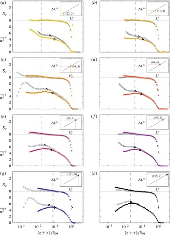
Smooth- and rough-wall streamwise variance and skewness comparisons at approximately matched friction Reynolds numbers ((a)
 ${\it\delta}_{99}^{+}\approx 4000$
. (b)
 ${\it\delta}_{99}^{+}\approx 2900$
. (c)
 ${\it\delta}_{99}^{+}\approx 9800$
. (d)
 ${\it\delta}_{99}^{+}\approx 5400$
. (e)
 ${\it\delta}_{99}^{+}\approx 17\,100$
. (f)
 ${\it\delta}_{99}^{+}\approx 7900$
. (g)
 ${\it\delta}_{99}^{+}\approx 4700$
. (h)
 ${\it\delta}_{99}^{+}\approx 22\,000$
). The inset in each figure shows the
 $k_{s}^{+}$
and
 ${\rm\Delta}U^{+}$
values of the rough-wall data in that figure. The figures are ordered from low
 $k_{s}^{+}$
to high
 $k_{s}^{+}$
. Dashed black lines mark the wall-normal locations of
 $3k_{s}/{\it\delta}_{99}$
. The symbols with thick black outlines show the location of the onset of inertial dynamics (
 $z_{I}$
) according to (2.4).

Figure 12 compares the smooth- and rough-wall streamwise variance and skewness at eight approximately matched friction Reynolds numbers in the range
 $2900\lesssim {\it\delta}_{99}^{+}\lesssim 22\,000$
. The figures are ordered from top to bottom according to the magnitude of
 $k_{s}^{+}$
. Matched Reynolds number comparisons such as these may avert, to some extent, the inherent friction Reynolds number trends of smooth- and rough-wall statistics that can cloud assessments of outer-layer similarity. However, it is difficult to apply any physical significance to such comparisons, other than that in each case the range of scales (between viscous and outer) present in the flow is approximately the same between the smooth and rough wall. Certainly, from a practical standpoint it may be more informative to compare smooth- and rough-wall boundary layers at matched
 $Re_{x}$
(
 $Re_{x}=xU_{\infty }/{\it\nu}$
, where
 $x$
is the distance from the laminar/turbulent trip) since such comparisons would demonstrate the effect of roughness in developing engineering flows such as on the hull of a ship or on the wing/fuselage of an aeroplane. The comparisons in figure 12 are presented simply because they reveal interesting trends in rough-wall-bounded flows. The aim here is to reveal any influence of roughness Reynolds number on low order rough-wall streamwise statistics in the absence of known friction Reynolds number trends. Primarily, the focus is on the outer region of the flow, with emphasis on the accuracy of Townsend’s wall-similarity hypothesis.
For all the transitionally rough flows (
 $k_{s}^{+}<$
70) in figure 12, apparent differences in the variance of the streamwise velocity fluctuations exist well into the outer layer when compared to the smooth wall at a matched Reynolds number. Note that this is consistent with the observed variations in
 $B_{1}$
for these transitionally rough surfaces. Of course, Townsend’s hypothesis is posed for high Reynolds number flows, and all the transitionally rough cases have
 ${\it\delta}_{99}^{+}\lesssim 10\,000$
. The results, however, indicate that, as the flow becomes fully rough, similarity in the variance of the streamwise velocity fluctuations in the outer layer emerges even for cases in which the friction Reynolds number is relatively low. For example, the
 ${\it\delta}_{99}^{+}\approx$
4700,
 $k_{s}^{+}=$
121 case (figure 12
g) displays similarity in the outer layer with the smooth-wall case at matching Reynolds number. To the authors’ knowledge, Townsend (Reference Townsend1956) hypothesised wall similarity across all flow conditions, including transitionally rough flows. Certainly, there are numerous instances in the existing literature where comparisons between smooth and transitionally rough boundary layers are made and outer-layer similarity is empirically found to hold (Schultz & Flack Reference Schultz and Flack2003, Reference Schultz and Flack2007; Wu & Christensen Reference Wu and Christensen2007; Allen et al.
Reference Allen, Shockling, Kunkel and Smits2007). The present results tentatively suggest, however, that the outer region of the inner-normalised streamwise velocity variance profile has a dependence on
 $k_{s}^{+}$
across the range of boundary layer and roughness parameters considered here. It is interesting to note that for the rough-wall data in figure 12(a) the drag balance measurements indicate an increase in the wall drag coefficient relative to the smooth wall at matched
 ${\it\delta}^{+}$
(presumably due to the pressure drag caused by the roughness elements). If, however, the ordinate of figure 12(a) is normalised by
 $U_{\infty }^{2}$
instead of
 $U_{{\it\tau}}^{2}$
, excellent collapse between the smooth- and rough-wall variance profiles is observed, indicating that for these data the strength of the streamwise turbulent fluctuations relative to the free stream velocity appears to be relatively unaffected by the rough surface. It is possible that this observation, and indeed the general trends with
 $k_{s}^{+}$
observed in figure 12, are caused by (or at least augmented by) experimental errors. For reasons discussed in detail in appendix A, it is not believed that this is the case.
Another observation from figure 12 is that the distance from the wall at which similarity begins to be observed – the edge of the roughness sublayer – in flows at high
 $k_{s}^{+}$
does not seem to scale in any straightforward manner on
 $k$
,
 $k_{s}$
or
 ${\it\delta}_{99}$
. This result stands in contrast to the findings of Raupach, Thom & Edwards (Reference Raupach, Thom and Edwards1980), Flack et al. (Reference Flack, Schultz and Shapiro2005) and Krogstad & Efros (Reference Krogstad and Efros2012) who assert that the region directly influenced by the roughness is confined to within approximately
 $5k$
of the wall. It should be noted, however, that the conclusions of these studies are based on lower Reynolds number flows in which the scale separation between
 $k$
and
 ${\it\delta}_{99}$
was much smaller than in the present case. Furthermore, other studies have documented rough-wall modifications to the Reynolds stresses that extend deep into the outer layer (Krogstadt & Antonia Reference Krogstadt and Antonia1999; Tachie et al.
Reference Tachie, Bergstrom and Balachandar2000; Keirsbulck et al.
Reference Keirsbulck, Labraga, Mazouz and Tournier2002). Based on the present results, the location at which inertial dynamics emerge,
 $z_{I}$
, for the rough-wall flows appears to be a better indicator of where similarity in the variance of the streamwise velocity fluctuations is observed, but only when
 $k_{s}^{+}$
is sufficiently large.
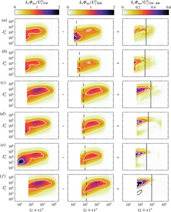
Smooth- and rough-wall premultiplied streamwise energy spectrograms at approximately matched
 ${\it\delta}_{99}^{+}$
, and the difference between them. Column 1, the smooth-wall spectrograms; Column 2, the rough-wall spectrograms; Column 3, subtraction of the rough-wall spectrograms from the smooth-wall spectrograms. Rows (a–f) present the spectrograms for most of the comparisons in figure 12 (
 ${\it\delta}_{99}^{+}\approx 4000,2900,17\,100,7900,4700,22\,000$
, respectively). Therefore
 $k_{s}^{+}$
increases from the top to the bottom of the figure. In the third column, contour lines are plotted at
 $k_{x}{\it\Phi}_{uu}/U_{{\it\tau}}^{2}|_{SW-RW}=\pm [0.15,0.3,0.45,0.6]$
. White lines represent positive contours and black lines represent negative contours. The dashed black vertical lines show the wall-normal location of
 $k_{s}^{+}$
and the solid black vertical lines show
 $z_{I}$
.

The comparisons of figure 12 are further scrutinised by considering the inner-normalised premultiplied streamwise turbulent energy spectrograms of selected smooth- and rough-wall datasets in figure 13. The same matched Reynolds number comparisons as those given in figure 12(a,b), (e–h) are presented. The first column in figure 13 shows the smooth-wall spectrograms; the second column shows the rough-wall spectrograms and the third column shows the difference between the smooth- and rough-wall spectrograms. In all comparisons, the Reynolds number is sufficient to reveal in the smooth-wall data wall-normal separation between the near-wall (predominantly small scale) energy peak and the logarithmic/outer-region (large scale) energy peak (Hutchins & Marusic Reference Hutchins and Marusic2007b
). In comparison (a) (
 ${\it\delta}_{99}^{+}\approx 4000$
and
 $k_{s}^{+}=22$
) the smooth- and rough-wall spectrograms are qualitatively similar, but the magnitude of the rough-wall energy at all scales across the boundary layer is reduced relative to that of the smooth wall. At higher roughness Reynolds numbers, previous studies have shown that the surface roughness causes a reduction in the near-wall energy peak relative to that of the smooth wall (Grass Reference Grass1971; Schultz & Flack Reference Schultz and Flack2007). This observation, however, is not made here due to the lack of resolved energy in this region. Farther into the boundary layer, figure 13(b–f) indicates the differences between the smooth- and rough-wall boundary layers appear to be primarily in the large scales of motion, i.e. motions that are several
 ${\it\delta}_{99}$
in length (note that a similar observation was also made by Monty et al. (Reference Monty, Allen, Lien and Chong2011) above a braille-type wall roughness). The magnitude of the difference between the smooth- and rough-wall large-scale near-wall motions seems to be related to the friction Reynolds number, with larger differences observed for flows with higher
 $k_{s}^{+}$
. It also appears that the effect of the rough-wall on the large-scale motions extends farther into the boundary layer (in wall units) with increasing Reynolds number (recall that figure 13 is ordered vertically according to
 $k_{s}^{+}$
, not
 ${\it\delta}_{99}^{+}$
). However, this trend (if real) is weak, and thus difficult to differentiate from experimental uncertainties. Note that in the third column of figure 13, it is apparent that
 $z_{I}$
(black lines) provides a reliable indicator of the wall-normal location beyond which there is little difference between the smooth- and rough-wall spectrograms. It then follows that this location scales with
 ${{\it\delta}_{99}^{+}}^{0.64}$
(as per (2.4)), perhaps explaining the apparent trend with
 ${\it\delta}_{99}^{+}$
.
4 Conclusions
A new and unique set of wind tunnel measurements have been used to empirically examine the streamwise velocity statistics and spectral intensities of turbulent boundary layers above a randomly distributed rough surface. Additionally, existing and newly acquired smooth-wall turbulent boundary layer data were employed to provide comparisons to the rough-wall results. The rough-wall measurements are unique in their range of roughness and boundary layer parameters (
 $2890\leqslant {\it\delta}_{99}^{+}\leqslant 29\,900$
,
 $26\leqslant k_{s}^{+}\leqslant 155$
and
 $28\leqslant {\it\delta}_{99}/k_{s}\leqslant 199$
), and in that they incorporate, at one streamwise location, direct measurements of the mean wall shear stress using a floating element drag balance. A new approach was introduced to determine
 $U_{{\it\tau}}$
at streamwise locations where drag balance data was not available. This approach uses the direct wall shear force measurements to construct the characteristic relationship between
 $k_{s}^{+}$
and
 ${\rm\Delta}U^{+}$
. It is assumed that this relationship is universal for a particular roughness, allowing
 $U_{{\it\tau}}$
to be estimated for data taken at any streamwise location and any free stream velocity. All data show self-consistent trends with friction and roughness Reynolds number.
The formulation proposed by Mehdi et al. (Reference Mehdi, Klewicki and White2013) was employed to estimate the wall-normal location of the onset of inertial mean dynamics,
 $z_{I}$
, in rough-wall flows. Aligning all rough-wall mean streamwise velocity profiles at this location revealed a distinct logarithmic region with constant slope (
 ${\it\kappa}$
) across all rough-wall profiles, extending from
 $z_{I}$
to
 $(z+{\it\epsilon})/{\it\delta}_{99}\approx 0.19$
. Such a region is consistent with an inertial sublayer of the flow, where the streamwise velocity is independent of first-order viscous effects. A similar log-linear region was revealed in the streamwise velocity variance across the same approximate bounds, as predicted by the attached eddy hypothesis of Townsend (Reference Townsend1976) (which is consistent with an inertial layer description). As was observed for the mean streamwise velocity, the slope (
 $A_{1}$
) of this region was approximately constant across all measurements. Thus, we provide evidence that the formulation of Mehdi et al. (Reference Mehdi, Klewicki and White2013) well predicts the wall-normal location of the onset of inertial dynamics in rough-wall flows. Additionally, the rough wall
 ${\it\kappa}$
and
 $A_{1}$
values agree to within experimental uncertainty with those recently determined for smooth-wall flows using high friction Reynolds number data from a range of facilities (Marusic et al.
Reference Marusic, Monty, Hultmark and Smits2013), suggesting similarity between the inertial region dynamics in smooth- and rough-wall flows.
Examination of the rough-wall mean streamwise velocity defect suggests that Townsend’s (Reference Townsend1956) wall-similarity hypothesis is an excellent approximation for this statistic across the full range of roughness and boundary layer parameters examined. Similarly, in the streamwise velocity skewness, good collapse is observed across all rough- and smooth-wall data beyond
 $(z+{\it\epsilon})/{\it\delta}_{99}\approx 0.2$
. In the streamwise velocity variance outer-layer collapse is observed for all flows with
 ${\it\delta}_{99}^{+}\gtrsim 14\,000$
. At low
 $k_{s}^{+}$
and intermediate
 ${\it\delta}_{99}^{+}$
, however, the outer region of the inner-normalised streamwise velocity variance seems to have some dependence on
 $k_{s}^{+}$
. At very low
 $k_{s}^{+}$
(
 $k_{s}^{+}\lesssim 30$
), the rough-wall streamwise velocity variance is qualitatively similar to that in smooth-wall flow at matched
 ${\it\delta}_{99}^{+}$
, but is attenuated across the entire boundary layer. Comparison of the rough- and smooth-wall spectrograms indicate that this attenuation acts equally at all wavelengths and wall-normal locations. The level of attenuation appears to decrease with increasing
 $k_{s}^{+}$
, such that, for fully rough flow, outer-layer collapse is observed for all available
 ${\it\delta}_{99}^{+}$
. That is, Townsend’s hypothesis also appears to be valid across all
 ${\it\delta}_{99}^{+}$
so long as the flow is fully rough. In this regime,
 $z_{I}$
appears to predict the edge of the roughness sublayer, indicating similarity across the entire inertial region of the flow. At moderate and high
 $k_{s}^{+}$
, the energy associated with near-wall streamwise motions is different between rough and smooth walls at matched friction Reynolds numbers. Much of the difference appears to reside in the large scales of motion (
 ${\it\lambda}^{+}=O({\it\delta}_{99})$
), with smaller scales (even those of the order of the roughness height,
 $k$
) apparently less affected. The magnitude of the difference appears to be related to
 $k_{s}^{+}$
, and the inner-normalised distance that this difference extends into the boundary layer seems to be a function of
 ${\it\delta}_{99}^{+}$
. A physical explanation for the trends described above is not yet known. The current measurements do not obtain data with low
 $k_{s}^{+}$
and high
 ${\it\delta}_{99}^{+}$
, which would be very valuable in elucidating the present results.
Acknowledgements
The authors wish to thank the Australian Research Council for the financial support of this research. M.P.S. would like to thank the U.S. Office of Naval Research for supporting his sabbatical visit to the University of Melbourne.
Appendix A. Are the trends with
 $k_{s}^{+}$
real?

The present results indicate that
 $k_{s}^{+}$
may play a larger role in outer-region rough-wall boundary layer dynamics than previous studies have indicated. Schultz & Flack (Reference Schultz and Flack2007), for example, report outer-layer collapse of the streamwise velocity variance for flows ranging from hydraulically smooth to fully rough. It is possible that the apparent importance of
 $k_{s}^{+}$
observed in the present study results from errors in determining wall friction velocity, or from changes in the tripping condition or streamwise pressure gradient effects at low speeds (which were required in the present study to generate flows with low
 $k_{s}^{+}$
). The following sections explain why it is difficult to use these explanations to refute the poor outer-layer collapse observed in the inner-normalised streamwise velocity variance at low
 $k_{s}^{+}$
.
The percentage difference between
 $U_{{\it\tau}}$
determined using the technique in § 2.4 (i.e. using the drag balance measurements), and that determined using an independent method. ‘MC’ refers to the modified Clauser (Reference Clauser1956) technique, and ‘TSS’ refers to the total shear stress method. The latter is only possible for the multi-wire measurements, for which
 $\overline{uw}$
profiles are available. Recall that the circular symbols represent data taken above the drag balance, for which
 $U_{{\it\tau}}$
is determined directly. The data are listed along the abscissa in the same order that they are presented in table 2. The hatched regions show
 ${\rm\Delta}U_{{\it\tau},MC}=\pm 5\,\%$
and
 ${\rm\Delta}U_{{\it\tau},TSS}=\pm 2\,\%$
.

A.1 Wall friction velocity
The rough-wall data with
 $k_{s}^{+}=22$
show the largest difference in the outer region of the inner-normalised streamwise velocity variance relative to a matched
 ${\it\delta}_{99}^{+}$
smooth-wall profile (see figure 12
a). These data are normalised by a wall friction velocity that was determined using direct drag balance measurements. While the uncertainty in the drag balance measurements certainly increases at the lower speeds required to generate low roughness Reynolds numbers (the rough-wall data in figure 12(a) is obtained at
 $U_{\infty }=4.7~\text{m}~\text{s}^{-1}$
), at
 $U_{\infty }\approx 5~\text{m}~\text{s}^{-1}$
the estimated error in
 $U_{{\it\tau}}$
is only
 $\pm 2.3\,\%$
(for a detailed discussion of the errors associated with the drag balance measurements see Baars et al. (Reference Baars, Squire, Talluru, Abbassi, Hutchins and Marusic2016)). It is possible to rescale the rough-wall profile in figure 12(a) to obtain outer-layer collapse with a matched
 ${\it\delta}_{99}^{+}$
smooth-wall profile. However, this requires a change in
 $U_{{\it\tau}}$
of approximately 9 % (note that changing
 $U_{{\it\tau}}$
changes
 ${\it\delta}_{99}^{+}$
, which in turn requires comparison to a different smooth-wall dataset). Additionally, collapse of the streamwise mean velocity to the rough-wall log-law (2.1) using the adjusted value for
 $U_{{\it\tau}}$
is then compromised unless
 ${\it\kappa}$
is changed by approximately 12 %. Furthermore, figure 14 shows the percentage difference between
 $U_{{\it\tau}}$
determined using the process in § 2.4, and that determined from two independent approaches. The first approach – hereafter called the modified Clauser (MC) method – determines
 $U_{{\it\tau}}$
and
 ${\rm\Delta}U^{+}$
to maximise agreement between the inner-normalised streamwise velocity and (2.1) across the inertial subrange. In the second approach – hereafter called the total shear stress (TSS) method – it is assumed that a nominally constant shear stress region exists in the inner part of the boundary layer which is equal to the wall shear stress. Therefore,
 $U_{{\it\tau}}$
can be calculated in this region using
 $$\begin{eqnarray}\displaystyle U_{{\it\tau}}\simeq \sqrt{{\it\nu}\frac{\partial U}{\partial z}-\overline{uw}}. & & \displaystyle\end{eqnarray}$$
Note that both the MC and TSS methods are common in the literature. Of course, the TSS method is only possible when
 $\overline{uw}$
profiles are available and hence is only used here for the multi-wire measurements. The
 $U_{{\it\tau}}$
values determined using the present approach (i.e. using the drag balance measurements – see § 2.4) agree with the MC method to within 5.3 %, and with the TSS method to within 1.9 % across all available rough-wall measurements. The agreement conveys little information regarding the error associated with each method (all three approaches have inherent errors). However, it is unlikely that three completely disassociated methods should produce such similar estimates of
 $U_{{\it\tau}}$
if those estimates are incorrect.
A.2 Low
$U_{\infty }$

A favourable streamwise pressure gradient or poorly stimulated boundary layer can exhibit inner-normalised streamwise velocity fluctuations that are attenuated relative to the zero pressure gradient equilibrium case (Harun et al.
Reference Harun, Monty, Mathis and Marusic2013; Marusic et al.
Reference Marusic, Chauhan, Kulandaivelu and Hutchins2015). In such flows the wake strength of the mean streamwise velocity is also significantly affected. In the present study, the streamwise pressure gradient in the wind tunnel was not assessed at the lowest operating speed (
 $U_{\infty }\approx 5$
). Additionally, it is possible that the smooth-wall trip (which generates canonical boundary layer evolution at
 $U_{\infty }=10{-}20~\text{m}~\text{s}^{-1}$
) understimulates the boundary layer at low speeds. However, in figure 6, excellent collapse of the streamwise velocity defect across all smooth- and rough-wall datasets is observed, indicating that there is little difference in the wake strength across all data presented, including the rough-wall profiles at low
 $k_{s}^{+}$
(and
 $U_{\infty }$
). Additionally, smooth-wall data taken at
 $U_{\infty }=4.7~\text{m}~\text{s}^{-1}$
are included in the comparisons in the present paper. These data agree well with smooth-wall data taken approximately matched
 ${\it\delta}_{99}^{+}$
but higher
 $U_{\infty }$
(see figures 5 and 6), suggesting that equilibrium flow is obtained in the wind tunnel even at these low operating speeds.