1 Introduction
When open dynamical systems are unstable, small amplitude disturbances superposed on a local base state are allowed to grow in space and/or time. In order to distinguish between these cases, one must identify the linear nature of the instability mechanism. This is achieved by analysing the asymptotic behaviour of wave packets generated by an impulse excitation of the linear and modal disturbance governing equation. Three possible scenarios emerge. If the disturbance envelope amplitude decays as it is advected downstream by the local base state, the system is convectively stable. Otherwise, it is unstable. In the latter case, two possible scenarios remain. If the disturbance envelope amplitude eventually decays in time when measured at a fixed location, the system is convectively unstable. Otherwise, the disturbance envelope amplitude will grow in time at any fixed location, which means the system is absolutely unstable. This understanding has an important impact on the development of control strategies for open dynamical systems. When these systems are convectively unstable, all disturbances eventually leave the domain of interest. In the absence of an external forcing that acts as a disturbance source, they eventually return to their original local base states. Hence, these systems are highly susceptible to control through low amplitude forcing. On the other hand, absolutely unstable systems allow any initially present disturbance to eventually grow in time, leading them away from their original local base state. In such cases, these systems become self-excited and more complex control strategies are required (Pier Reference Pier2009).
Within the context of hydrodynamic instabilities, Betchov & Criminale (Reference Betchov and Criminale1966) were among the first to find singularities in an eigenvalue problem when studying the linear stability of inviscid jets and wakes. Soon afterwards, Gaster (Reference Gaster1968) recognised that these singularities appeared as saddle points in a complex wavenumber plane when analysing the impulse response of the eigenvalue problem. Furthermore, he noticed that the wave packet generated by this pulse was physically meaningful when its group velocity was zero, which could indicate when spatially growing disturbances would start growing in time. These ideas were first applied to distinguish between convective and absolute instabilities in fluid dynamics by Thacker (Reference Thacker1975) for the analysis of Gulf Stream meanders as well as Merkine (Reference Merkine1977) for the study of baroclinic eddies. However, they did not develop these ideas and concepts, but instead drew from the theoretical foundations underlying these notions that were already extensively developed in the field of plasma instabilities. Popular among them were the collision criteria devised by Briggs (Reference Briggs1964) and the convective/absolute instability description by Bers (Reference Bers1975). A detailed account of this development in plasma instabilities was reviewed by Bers (Reference Bers1983) whereas a survey on the use of these tools in the field of hydrodynamic instabilities was written by Huerre & Monkewitz (Reference Huerre and Monkewitz1990). The nomenclature used here follows that of Gaster (Reference Gaster1968), for the general term singularity in eigenvalue problems, and Huerre & Monkewitz (Reference Huerre and Monkewitz1990), who refer to the absolute frequency and wavenumber as branch and saddle points, respectively. They also use the term pinch for saddle points as well as cusp for branch points that satisfy causality.
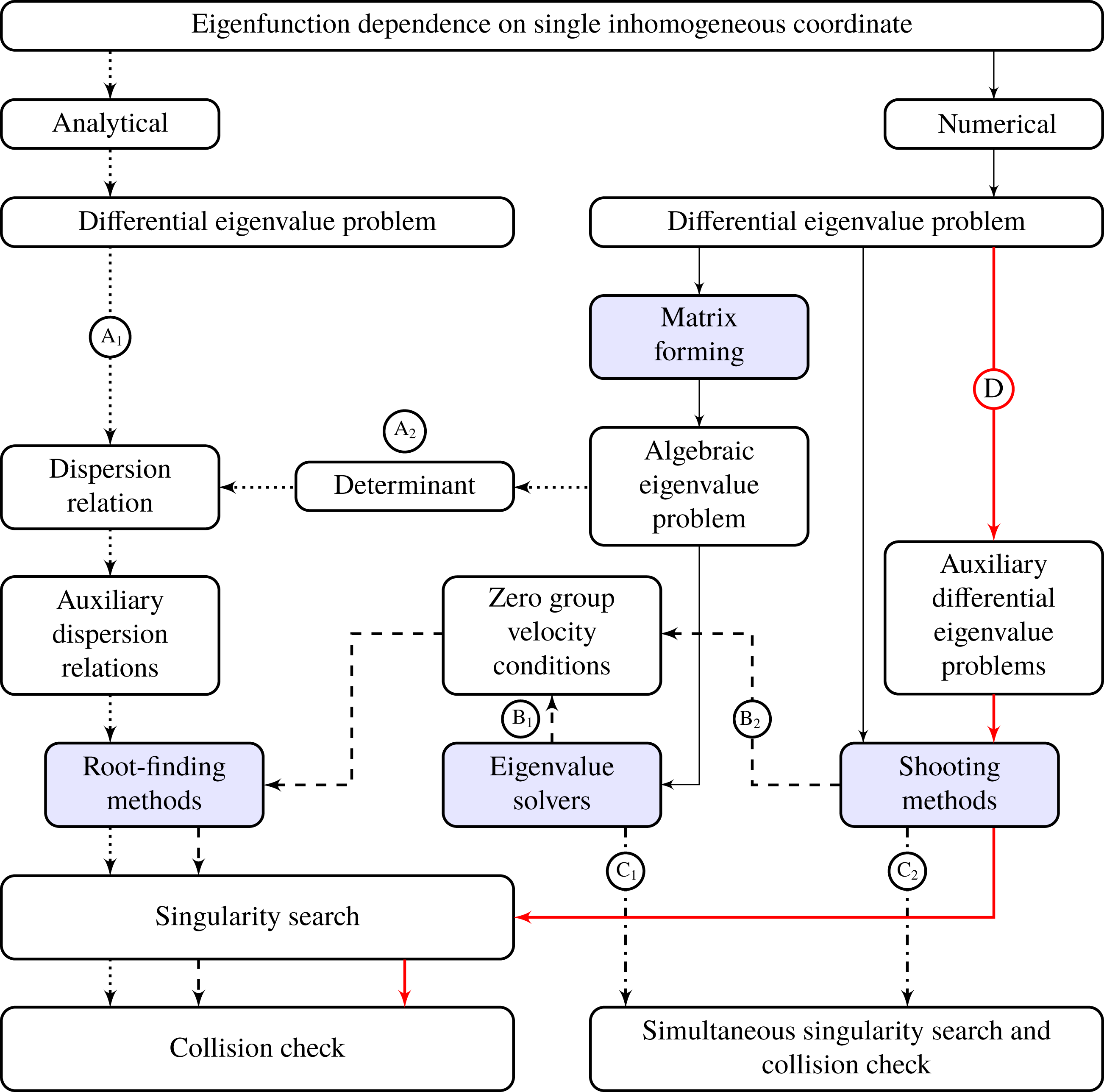
Theory (white blocks) and numerics (light blue blocks) flowchart to illustrate some of the most common methods used to perform local and linear absolute stability analyses (paths
 $\text{A}$
to
 $\text{C}$
in non-solid black) as well as the new method proposed here (path
 $\text{D}$
in solid red).

The original demonstration of a transition to absolute instability required proof of causality, i.e. proof that the contours of the integration that defines the linear impulse response of a system can be deformed into a steepest descent integration path containing the singularity. Due to the inherent difficulties in this proof, early attempts to find the parametric conditions where a local base state transitions from convectively to absolutely unstable relied on the collision criterion instead. This graphical proof was used to locate saddle points on the complex wavenumber plane that were in fact pinching points, i.e. that were formed by the collision between downstream and upstream propagating spatial branches that satisfy the eigenvalue problem. The most common paths towards this graphical proof of causality are illustrated in figure 1, where white and light blue boxes represent theoretical and numerical steps, respectively. Paths
 $\text{C}_{1}$
and
 $\text{C}_{2}$
in this figure respectively indicate the use of matrix forming and shooting methods to solve differential eigenvalue problems in order to evaluate the collision criterion. The former has become more popular (Hwang & Choi Reference Hwang and Choi2006; Brevdo & Ruderman Reference Brevdo and Ruderman2009), whereas the latter was very common in early linear stability analyses, such as those of planar mixing layers (Huerre & Monkewitz Reference Huerre and Monkewitz1985), flows around bluff bodies (Monkewitz & Nguyen Reference Monkewitz and Nguyen1987), hot jets (Monkewitz & Sohn Reference Monkewitz and Sohn1988), boundary layers on rotating disks (Lingwood Reference Lingwood1995, Reference Lingwood1997a
) and several other problems. A common feature among these studies is their focus on two-dimensional instabilities. This terminology is used here to emphasise that wave packets are allowed to propagate in a single homogenous direction. Since only one direction is inhomogeneous in these references, any variation in the remaining homogeneous direction is prescribed through its respective wavenumber. The former five references prescribe it to zero whereas the latter two references prescribe it to a positive number. For this reason, the latter two are named pseudo-two-dimensional absolute instability analyses from this point on. Nevertheless, any search for singularities always considers only a single wavenumber plane when dealing with two- or pseudo-two-dimensional instabilities. The extension of this transition framework towards three-dimensional instabilities was derived by Brevdo (Reference Brevdo1991). In this case, wave packets are allowed to propagate in both homogeneous directions and the graphical search for singularities must consider both wavenumber planes simultaneously. However, he noted the greater difficulty in proving the existence of a steepest descent surface, as compared to its line counterpart in two dimensions, recommending the application of the collision criterion instead. Nevertheless, even this criterion is numerically expensive in two dimensions and prohibitive in three dimensions. It is much cheaper to only search for singularities using the zero group velocity conditions, which can be done using asymptotic expansions that are known since the work of Benjamin (Reference Benjamin1961) and Criminale & Kovasznay (Reference Criminale and Kovasznay1962), without performing a collision check to verify causality. This led to the development of techniques that track the movement of singularities as one parameter is varied, where the most popular ones are known as continuation methods. Well-known examples of such methods were developed by Deissler (Reference Deissler1987), Brevdo (Reference Brevdo1995) and Brevdo et al. (Reference Brevdo, Laure, Dias and Bridges1999) for two-dimensional instabilities and extended by Oertel & Delfs (Reference Oertel and Delfs1995) and Koch (Reference Koch2002) to three-dimensional instabilities. They numerically calculate the group velocities, often based on the frequency dependence on the wavenumbers obtained from a temporal stability analysis, and locate the singularities with root-finding methods. It is important to note that these methods perform their temporal stability calculations using either algebraic (with eigenvalue solvers) or differential (with shooting methods) eigenvalue problems, illustrated by paths
 $\text{B}_{1}$
and
 $\text{B}_{2}$
in figure 1, respectively. Causality is verified a posteriori for a small sample of singularities in order to reduce computational cost. Nevertheless, this sample is usually chosen to be large enough to generate sufficient confidence that the entire set satisfies causality. A review of continuation methods was presented by Suslov (Reference Suslov2006), who also proposed a more efficient alternative, but only two-dimensional calculations were presented. Despite their widespread use, a word of caution about collision checks, steepest descent methods and continuation methods is required. Lingwood (Reference Lingwood1997b
) has shown that it might not be an easy task to prove that the inversion contour can be deformed into the steepest descent path for any given singularity. Furthermore, Brevdo et al. (Reference Brevdo, Laure, Dias and Bridges1999) have shown that continuation methods must be used with care because they cannot capture singularities that are not connected by continuity. These difficulties in the search for three-dimensional singularities often force researchers to search instead for two-dimensional (zero either streamwise or spanwise wavenumber) ones, as done by Hirata et al. (Reference Hirata, Alves, Delenda and Ouarzazi2015), or pseudo two-dimensional (non-zero but real spanwise wavenumber) ones, as done by Lingwood (Reference Lingwood1997c
). However, this compromise can lead to misleading results. Brevdo & Ruderman (Reference Brevdo and Ruderman2009) found in their study of mixed convection in a porous medium that two-dimensional longitudinal (zero streamwise wavenumber) modes became absolutely unstable under the same conditions that Brevdo (Reference Brevdo2009) found three-dimensional longitudinal modes to always be convectively unstable. Furthermore, Alves & Barletta (Reference Alves and Barletta2015) found in a similar problem, but for dilatant fluids modelled by a power law, that the onset of absolute instability switched in a discontinuous manner between transverse (zero spanwise wavenumber) and longitudinal modes as the Péclet number was increased in a three-dimensional instability analysis. On the other hand, they found that this switch was smooth, going through all possible oblique modes in between, in a pseudo-two-dimensional instability analysis. All these cautionary examples show the importance of distinguishing three- and two-dimensional singularities.
As mentioned by Koch (Reference Koch2002), the numerical difficulties associated with continuation methods are an issue because they are the best known methods available for the search of three-dimensional singularities when dealing with differential eigenvalue problems. This difficulty in locating three-dimensional absolutely unstable singularities even affects the WKBJ reconstruction of global modes, according to Martinand, Carrière & Monkewitz (Reference Martinand, Carrière and Monkewitz2004). Whenever a dispersion relation can be found, auxiliary dispersion relations can be derived using zero group velocity conditions and the search for singularities reduces to solving the resulting system of algebraic equations with root-finding methods. Many examples can be found in the literature, such as the studies by Chomaz, Couairon & Julien (Reference Chomaz, Couairon and Julien1999), Delache, Ouarzazi & Combarnous (Reference Delache, Ouarzazi and Combarnous2007), Hirata & Ouarzazi (Reference Hirata and Ouarzazi2010) and Alves & Barletta (Reference Alves and Barletta2015). These examples share a common feature, their dispersion relations are simple analytical expressions due to the analytical form of their eigenfunction dependence on their single inhomogeneous coordinate. This is the path
 $\text{A}_{1}$
illustrated in figure 1. The use of such auxiliary dispersion relations is so effective that some researchers try to avoid the use of steepest descent, collision checks or continuation methods to search for singularities from differential eigenvalue problems. They use instead a matrix forming approach to transform the differential eigenvalue problem into an algebraic eigenvalue problem. Requiring its determinant to be zero for a non-trivial solution to exist also leads to a dispersion relation, although it is a significantly more complex analytical expression. In doing so, the zero group velocity conditions can once again be used to generate auxiliary dispersion relations and the search for singularities can be performed with root-finding methods. Such a matrix forming approach was employed by Carrière & Monkewitz (Reference Carrière and Monkewitz1999) using Galerkin/collocation methods and recently in still ongoing studies by Brandao, Alves & Barletta (Reference Brandao, Alves and Barletta2014, Reference Brandao, Alves and Barletta2015) using a generalised Fourier transform. This is the path
 $\text{A}_{2}$
illustrated in figure 1. However, as noted by Brevdo (Reference Brevdo2009), solving this system of equations can be a rather involved computational task. In fact, Hirata et al. (Reference Hirata, Alves, Delenda and Ouarzazi2015) attempted to solve their problem through path
 $\text{A}_{2}$
using a Galerkin method based matrix forming, but the very high symbolic computational cost associated with deriving the auxiliary dispersion relations using the zero group velocity conditions did not allow numerically converged results to be reached. These examples reveal that a reliable method to extract three-dimensional singularities from differential eigenvalue problems has yet to be found.
In the present paper, a novel procedure is put forward that enables the search for two- and three-dimensional singularities in differential eigenvalue problems without having to resort to determinants (path
 $\text{A}_{2}$
), numerical group velocity calculations (paths
 $\text{B}$
) or collision checks (paths
 $\text{C}$
). It applies the ideas associated with adjoint sensitivity analysis (Luchini & Bottaro Reference Luchini and Bottaro2014) to boundary value problems so the zero group velocity conditions can be used to generate auxiliary differential eigenvalue problems, analogous to the auxiliary dispersion relations from path
 $\text{A}$
. This coupled system of equations now contains two and three differential eigenvalue problems for two- and three-dimensional singularity searches, respectively, which can be solved using the same shooting methods used to solve the direct differential eigenvalue problem (in paths
 $\text{B}_{2}$
and
 $\text{C}_{2}$
). Path
 $\text{D}$
in figure 1 illustrates this novel procedure. When coupled with adjoint analysis (Luchini & Bottaro Reference Luchini and Bottaro2014), this procedure can also calculate the group velocity of the modes within both spatial branches involved in the collision that forms the singularity. In doing so, it can determine the propagation directions of these two- and three-dimensional branches involved in the collision. Well-known two-, pseudo-two- and three-dimensional instabilities are solved to demonstrate the capabilities of this novel procedure. Fluid properties are considered constant in these test cases, but allowing them to vary does not modify the proposed methodology in any significant way.
2 Mathematical formulation
2.1 Differential eigenvalue problems
Consider an open dynamical system in the form of
 $$\begin{eqnarray}\displaystyle \frac{\unicode[STIX]{x2202}\boldsymbol{q}}{\unicode[STIX]{x2202}t}=\boldsymbol{f}(\boldsymbol{q}), & & \displaystyle\end{eqnarray}$$
where
 $\boldsymbol{f}(\boldsymbol{q}_{b})=0$
yields its nonlinear steady state and its state variable vector
 $\boldsymbol{q}(\boldsymbol{x},t)$
can be decomposed into the usual local, one-dimensional and modal form
 $$\begin{eqnarray}\displaystyle \boldsymbol{q}(\boldsymbol{x},t)=\boldsymbol{q}_{b}(z)+\unicode[STIX]{x1D716}\boldsymbol{q}_{n}(z)\text{e}^{\text{i}(\unicode[STIX]{x1D6FC}x+\unicode[STIX]{x1D6FD}y-\unicode[STIX]{x1D714}t)}, & & \displaystyle\end{eqnarray}$$
where
 $\unicode[STIX]{x1D716}$
is a disturbance amplitude parameter,
 $\text{i}$
is the imaginary unit,
 $x$
and
 $y$
are the streamwise and spanwise coordinates, respectively,
 $z$
is the only inhomogeneous coordinate and
 $t$
is time. Furthermore, the local base state vector is
 $\boldsymbol{q}_{b}(z)$
and the disturbance normal mode is defined by its eigenfunction vector
 $\boldsymbol{q}_{n}(z)$
and its eigenvalues, given by the frequency
 $\unicode[STIX]{x1D714}$
as well as streamwise and spanwise wavenumbers
 $\unicode[STIX]{x1D6FC}$
and
 $\unicode[STIX]{x1D6FD}$
, respectively. When substituting decomposition (2.2) into the dynamical system governing equation (2.1) and collecting the linear terms of
 $O(\unicode[STIX]{x1D716})$
, an ordinary differential system of equations with respect to
 $z$
is obtained for
 $\boldsymbol{q}_{n}(z)$
. It is written here as
 $$\begin{eqnarray}\displaystyle {\mathcal{L}}\boldsymbol{q}_{n}=0, & & \displaystyle\end{eqnarray}$$
where
 ${\mathcal{L}}={\mathcal{L}}(\unicode[STIX]{x1D6FC},\unicode[STIX]{x1D6FD},\unicode[STIX]{x1D714};{\mathcal{R}})$
is a linear and homogeneous differential operator that depends on all eigenvalues and
 ${\mathcal{R}}$
, which can represent either one or more control parameters. Examples include the Reynolds, Prandtl, Péclet and Rayleigh numbers. Equation (2.3) could also be a partial differential equation, if one assumes
 $\boldsymbol{q}(\boldsymbol{x},t)=\boldsymbol{q}_{b}(y,z)+\unicode[STIX]{x1D716}\boldsymbol{q}_{n}(y,z)\text{e}^{\text{i}(\unicode[STIX]{x1D6FC}x-\unicode[STIX]{x1D714}t)}$
instead of (2.2). Under such constraints, a local but two-dimensional modal analysis would be performed, also known as a spatial bi-global analysis in the literature (Theofilis Reference Theofilis2003, Reference Theofilis2011). An example of such a local two-dimensional analysis is the case of an eccentric Taylor–Couette–Poiseuille flow recently studied by Leclercq, Pier & Scott (Reference Leclercq, Pier and Scott2014). In any case, equation (2.3) is still a differential eigenvalue problem. The different information about two- and three-dimensional singularities, as well as group velocities, one can extract from this equation using shooting methods is the focus of the present paper.
2.2 Dispersion relations
Matrix forming equation (2.3) can be used instead to generate dispersion relations. However, this approach is often unfeasible and, hence, should be avoided when searching for linear absolute instabilities. In order to better illustrate why, path
 $\text{A}_{2}$
from figure 1 is discussed now. Applying an arbitrary spatial discretisation to (2.3) yields
 $$\begin{eqnarray}\displaystyle \unicode[STIX]{x1D647}q_{n}=0, & & \displaystyle\end{eqnarray}$$
where
 $\unicode[STIX]{x1D647}\in \mathbb{C}^{(N\times N)}$
and
 $q_{n}\in \mathbb{C}^{(N)}$
are the discrete and complex matrix and eigenvector versions of differential operator
 ${\mathcal{L}}$
and eigenfunction
 $\boldsymbol{q}_{n}$
, respectively, with
 $N$
defining the arbitrary size of this system. The first dispersion relation comes from the necessary condition for the existence of non-trivial solutions for
 $q_{n}$
in (2.4), i.e.
 $$\begin{eqnarray}\displaystyle \text{det}(\unicode[STIX]{x1D647})=0, & & \displaystyle\end{eqnarray}$$
where
 $\text{det}(\unicode[STIX]{x1D647})$
is the determinant of
 $\unicode[STIX]{x1D647}$
. The auxiliary dispersion relations needed to search for singularities then come from
 $$\begin{eqnarray}\displaystyle \frac{\unicode[STIX]{x2202}\text{det}(\unicode[STIX]{x1D647})}{\unicode[STIX]{x2202}\unicode[STIX]{x1D6FC}}=0\quad \text{with}~\frac{\unicode[STIX]{x2202}\unicode[STIX]{x1D714}}{\unicode[STIX]{x2202}\unicode[STIX]{x1D6FC}}=0 & & \displaystyle\end{eqnarray}$$
and
 $$\begin{eqnarray}\displaystyle \frac{\unicode[STIX]{x2202}\text{det}(\unicode[STIX]{x1D647})}{\unicode[STIX]{x2202}\unicode[STIX]{x1D6FD}}=0\quad \text{with}~\frac{\unicode[STIX]{x2202}\unicode[STIX]{x1D714}}{\unicode[STIX]{x2202}\unicode[STIX]{x1D6FD}}=0, & & \displaystyle\end{eqnarray}$$
for two-, pseudo-two- and three-dimensional instabilities. Whenever (2.3) is normal, i.e.
 $\boldsymbol{q}_{n}(z)$
has a modal dependence on
 $z$
,
 $\unicode[STIX]{x1D647}$
is a diagonal matrix. In this case,
 $\text{det}(\unicode[STIX]{x1D647})$
is the product of its diagonal elements, i.e. the algebraic eigenvalue problem defined in (2.4) is a decoupled system of algebraic equations. Hence, the symbolic computational cost of generating (2.5) to (2.7) is essentially negligible. On the other hand, if (2.3) is non-normal,
 $\unicode[STIX]{x1D647}$
is no longer diagonal and the algebraic eigenvalue problem now represents a coupled system of equations. Hence, the symbolic computational cost of generating
 $\text{det}(\unicode[STIX]{x1D647})$
and its derivatives with respect to the wavenumbers is much higher. In fact, this cost can be prohibitively high even for moderate degrees of coupling and model complexity, as mentioned in § 1. Numerically evaluating this determinant and its derivatives instead usually speeds up computations, but in general this is not enough to allow path
 $\text{A}_{2}$
to be competitive with paths
 $\text{B}$
and
 $\text{D}$
in figure 1.
2.3 Sensitivity analysis
In order to avoid the potentially prohibitive symbolic/numeric computational cost associated with deriving the dispersion relations required in the search for singularities using (2.5), one must search for them using differential eigenvalue problems in the form of (2.3) instead. In the present paper, a shooting method is employed to solve this equation. Doing so yields two complex solutions: the eigenfunction vector
 $\boldsymbol{q}_{n}(z)$
and one eigenvalue, for prescribed values of the remaining eigenvalues. All control parameters are prescribed as well. When performing a temporal stability analysis,
 $\unicode[STIX]{x1D714}$
is the complex eigenvalue being solved for prescribed real values of the remaining eigenvalues
 $\unicode[STIX]{x1D6FC}$
and
 $\unicode[STIX]{x1D6FD}$
. On the other hand, when performing a spatial stability analysis,
 $\unicode[STIX]{x1D6FC}$
is the complex eigenvalue being solved for prescribed real values of the remaining eigenvalues
 $\unicode[STIX]{x1D714}$
and
 $\unicode[STIX]{x1D6FD}$
.
Since
 $\unicode[STIX]{x1D714}$
,
 $\unicode[STIX]{x1D6FC}$
and
 $\unicode[STIX]{x1D6FD}$
are coupled at these singularities, auxiliary differential eigenvalue problems must be solved simultaneously with (2.3) for these eigenvalues. Taking the derivative of this equation with respect to
 $\unicode[STIX]{x1D6FC}$
and
 $\unicode[STIX]{x1D6FD}$
, respectively, leads to
 $$\begin{eqnarray}\displaystyle {\mathcal{L}}\boldsymbol{q}_{\unicode[STIX]{x1D6FC}}={\mathcal{S}}_{\unicode[STIX]{x1D6FC}}\quad \text{with }{\mathcal{S}}_{\unicode[STIX]{x1D6FC}}=-{\mathcal{L}}_{\unicode[STIX]{x1D6FC}}\boldsymbol{q}_{n} & & \displaystyle\end{eqnarray}$$
and
 $$\begin{eqnarray}\displaystyle {\mathcal{L}}\boldsymbol{q}_{\unicode[STIX]{x1D6FD}}={\mathcal{S}}_{\unicode[STIX]{x1D6FD}}\quad \text{with }{\mathcal{S}}_{\unicode[STIX]{x1D6FD}}=-{\mathcal{L}}_{\unicode[STIX]{x1D6FD}}\boldsymbol{q}_{n}, & & \displaystyle\end{eqnarray}$$
where
 $\boldsymbol{q}_{\unicode[STIX]{x1D6FC}}=\unicode[STIX]{x2202}\boldsymbol{q}_{n}/\unicode[STIX]{x2202}\unicode[STIX]{x1D6FC}$
,
 $\boldsymbol{q}_{\unicode[STIX]{x1D6FD}}=\unicode[STIX]{x2202}\boldsymbol{q}_{n}/\unicode[STIX]{x2202}\unicode[STIX]{x1D6FD}$
,
 ${\mathcal{L}}_{\unicode[STIX]{x1D6FC}}=\unicode[STIX]{x2202}{\mathcal{L}}/\unicode[STIX]{x2202}\unicode[STIX]{x1D6FC}$
and
 ${\mathcal{L}}_{\unicode[STIX]{x1D6FD}}=\unicode[STIX]{x2202}{\mathcal{L}}/\unicode[STIX]{x2202}\unicode[STIX]{x1D6FD}$
. Furthermore,
 ${\mathcal{L}}_{\unicode[STIX]{x1D6FC}}={\mathcal{L}}_{\unicode[STIX]{x1D6FC}}(\unicode[STIX]{x1D6FC},\unicode[STIX]{x1D6FD},\unicode[STIX]{x1D714},\unicode[STIX]{x2202}\unicode[STIX]{x1D714}/\unicode[STIX]{x2202}\unicode[STIX]{x1D6FC};{\mathcal{R}},\unicode[STIX]{x2202}{\mathcal{R}}/\unicode[STIX]{x2202}\unicode[STIX]{x1D6FC})$
and
 ${\mathcal{L}}_{\unicode[STIX]{x1D6FD}}={\mathcal{L}}_{\unicode[STIX]{x1D6FD}}(\unicode[STIX]{x1D6FC},\unicode[STIX]{x1D6FD},\unicode[STIX]{x1D714},\unicode[STIX]{x2202}\unicode[STIX]{x1D714}/\unicode[STIX]{x2202}\unicode[STIX]{x1D6FD};{\mathcal{R}},\unicode[STIX]{x2202}{\mathcal{R}}/\unicode[STIX]{x2202}\unicode[STIX]{x1D6FD})$
are also linear and homogeneous operators, where
 $\boldsymbol{q}_{n}(z)$
,
 $\unicode[STIX]{x1D714}$
and
 ${\mathcal{R}}$
are allowed to depend on
 $\unicode[STIX]{x1D6FC}$
and
 $\unicode[STIX]{x1D6FD}$
. The latter dependence is included here to generalise this procedure to calculate critical points for the onset of convective instabilities (Alves, Hirata & Ouarzazi Reference Alves, Hirata and Ouarzazi2016), even though this paper is focussed on absolute instabilities. Equations (2.8) and (2.9) are solved within the same shooting methodology used to solve for (2.3). Since they also yield two complex solutions each, one eigenfunction and one eigenvalue, these three equations can be used to find three eigenfunctions and three eigenvalues for three-dimensional instabilities. Two eigenvalues and two eigenfunctions can similarly be found for two- and pseudo-two-dimensional instabilities, where either (2.8) or (2.9) is dropped.
At this point, it is important to justify our focus on differential equations and shooting methods instead of matrix forming and generalised eigenvalue solvers. Both approaches are widely used in the literature. The former solves (2.3) whereas the latter solves (2.4), usually in the form of
 $\unicode[STIX]{x1D63C}q_{n}=\unicode[STIX]{x1D714}\unicode[STIX]{x1D63D}q_{n}$
for a temporal stability analysis. A nonlinear eigenvalue problem appears, however, if a spatial stability analysis is desired instead. For instance, a typical example of the form (2.4) takes in such an analysis is
 $\unicode[STIX]{x1D63C}q_{n}=\unicode[STIX]{x1D6FC}\unicode[STIX]{x1D63D}_{1}q_{n}+\unicode[STIX]{x1D6FC}^{2}\unicode[STIX]{x1D63D}_{2}q_{n}$
. This requires linearisation, which is achieved with the companion matrix method (Bridges & Morris Reference Bridges and Morris1984). Matrices
 $\unicode[STIX]{x1D63C}$
and
 $\unicode[STIX]{x1D63D}$
come from
 $\unicode[STIX]{x1D647}$
. In order to directly solve for singularities using this approach, however, one needs to apply matrix forming to (2.8) and (2.9). Doing so to the former leads to (2.23), discussed later on in a different context. This yields a system of three coupled generalised eigenvalue problems with three different but coupled eigenvalues. At the present time, it is not clear how such a problem can be solved in an efficient manner.
Although (2.8) and (2.9) were obtained from (2.3) in the same way (2.6) and (2.7) were obtained from (2.5), their derivation is closely related to sensitivity analysis (Luchini & Bottaro Reference Luchini and Bottaro2014). In such an analysis, one introduces small variations in a generalised eigenvalue problem, usually in the form of (2.4), and uses the adjoint eigenvector
 $q_{n}^{+}$
of the direct eigenvector
 $q_{n}$
to identify gradients between different problem variables and/or parameters. Equations (2.8) and (2.9) can then be understood as the differential version of this analysis, based on (2.3) instead, where gradients with respect to the wavenumbers are sought. Although sensitivity studies of global modes are based on algebraic equations, their differential counterparts have been used for similar studies of local (Bottaro, Corbett & Luchini Reference Bottaro, Corbett and Luchini2003) and global modes (Juniper & Pier Reference Juniper and Pier2015). The present method, however, is distinct in two ways. The first one is that the adjoint eigenfunction
 $\boldsymbol{q}_{n}^{+}(z)$
of the direct eigenfunction
 $\boldsymbol{q}_{n}(z)$
does not have to be obtained in order to solve for (2.8) and (2.9), but wavenumber sensitivity eigenfunctions
 $\boldsymbol{q}_{\unicode[STIX]{x1D6FC}}(z)$
and
 $\boldsymbol{q}_{\unicode[STIX]{x1D6FD}}(z)$
have to be obtained instead. The second way is that a normalisation, introduced in a traditional sensitivity analysis based on
 $q_{n}^{+}(z)$
, is also required in (2.8) and (2.9). Since they are also eigenvalue problems,
 $\boldsymbol{q}_{\unicode[STIX]{x1D6FC}}(z)$
and
 $\boldsymbol{q}_{\unicode[STIX]{x1D6FD}}(z)$
are undetermined with respect to one integration constant each, which means normalisations are required to remove them.
Adjoints may not be required to solve (2.8) and (2.9), but they are necessary to guarantee that a solution to these equations exists. Using
 $\langle u,v\rangle$
as the notation for a yet to be defined inner product between two arbitrary complex functions
 $u(z)$
and
 $v(z)$
, an adjoint differential eigenvalue problem operator
 ${\mathcal{L}}^{\ast }$
can be defined using either
 $$\begin{eqnarray}\displaystyle \langle {\mathcal{L}}\boldsymbol{q}_{\unicode[STIX]{x1D6FC}},\boldsymbol{q}_{n}^{+}\rangle =\langle \boldsymbol{q}_{\unicode[STIX]{x1D6FC}},{\mathcal{L}}^{\ast }\boldsymbol{q}_{n}^{+}\rangle & & \displaystyle\end{eqnarray}$$
or
 $$\begin{eqnarray}\displaystyle \langle {\mathcal{L}}\boldsymbol{q}_{\unicode[STIX]{x1D6FD}},\boldsymbol{q}_{n}^{+}\rangle =\langle \boldsymbol{q}_{\unicode[STIX]{x1D6FD}},{\mathcal{L}}^{\ast }\boldsymbol{q}_{n}^{+}\rangle , & & \displaystyle\end{eqnarray}$$
where
 $\ast$
means conjugate transpose, to produce
 $\boldsymbol{q}_{n}^{+}(z)$
, an adjoint of
 $\boldsymbol{q}_{n}(z)$
, from
 $$\begin{eqnarray}\displaystyle {\mathcal{L}}^{\ast }\boldsymbol{q}_{n}^{+}=0, & & \displaystyle\end{eqnarray}$$
which is the adjoint version of (2.3). Using the linear and inhomogeneous equations (2.8) and (2.9), as well as (2.12), it is possible to simplify (2.10) and (2.11) to
 $$\begin{eqnarray}\displaystyle \langle {\mathcal{S}}_{\unicode[STIX]{x1D6FC}},\boldsymbol{q}_{n}^{+}\rangle =0 & & \displaystyle\end{eqnarray}$$
and
 $$\begin{eqnarray}\displaystyle \langle {\mathcal{S}}_{\unicode[STIX]{x1D6FD}},\boldsymbol{q}_{n}^{+}\rangle =0, & & \displaystyle\end{eqnarray}$$
known as solvability conditions. They derive from the Fredholm alternative theorem, which states that the inhomogeneous term of a linear equation, e.g.
 ${\mathcal{S}}_{\unicode[STIX]{x1D6FC}}$
or
 ${\mathcal{S}}_{\unicode[STIX]{x1D6FD}}$
, must be orthogonal to the adjoint solution of the corresponding homogeneous equation, e.g.
 $\boldsymbol{q}_{n}^{+}$
, for the existence of non-trivial solutions to the inhomogeneous equation, e.g.
 $\boldsymbol{q}_{\unicode[STIX]{x1D6FC}}$
or
 $\boldsymbol{q}_{\unicode[STIX]{x1D6FD}}$
.
Equations (2.13) and (2.14) can now be used to calculate the group velocities
 $\unicode[STIX]{x2202}\unicode[STIX]{x1D714}/\unicode[STIX]{x2202}\unicode[STIX]{x1D6FC}$
and
 $\unicode[STIX]{x2202}\unicode[STIX]{x1D714}/\unicode[STIX]{x2202}\unicode[STIX]{x1D6FD}$
, which naturally appear within
 ${\mathcal{L}}_{\unicode[STIX]{x1D6FC}}$
and
 ${\mathcal{L}}_{\unicode[STIX]{x1D6FD}}$
, respectively. Since these operators can always be re-written as
 ${\mathcal{L}}_{\unicode[STIX]{x1D6FC}}={\mathcal{L}}_{\unicode[STIX]{x1D6FC}}^{_{(0)}}-{\mathcal{L}}_{\unicode[STIX]{x1D6FC}}^{_{(1)}}\unicode[STIX]{x2202}\unicode[STIX]{x1D714}/\unicode[STIX]{x2202}\unicode[STIX]{x1D6FC}$
and
 ${\mathcal{L}}_{\unicode[STIX]{x1D6FD}}={\mathcal{L}}_{\unicode[STIX]{x1D6FD}}^{_{(0)}}-{\mathcal{L}}_{\unicode[STIX]{x1D6FD}}^{_{(1)}}\unicode[STIX]{x2202}\unicode[STIX]{x1D714}/\unicode[STIX]{x2202}\unicode[STIX]{x1D6FD}$
, equations (2.13) and (2.14) can be correspondingly re-written to yield
 $$\begin{eqnarray}\displaystyle \frac{\unicode[STIX]{x2202}\unicode[STIX]{x1D714}}{\unicode[STIX]{x2202}\unicode[STIX]{x1D6FC}}=\frac{\langle {\mathcal{L}}_{\unicode[STIX]{x1D6FC}}^{_{(0)}}\boldsymbol{q}_{n},\boldsymbol{q}_{n}^{+}\rangle }{\langle {\mathcal{L}}_{\unicode[STIX]{x1D6FC}}^{_{(1)}}\boldsymbol{q}_{n},\boldsymbol{q}_{n}^{+}\rangle } & & \displaystyle\end{eqnarray}$$
and
 $$\begin{eqnarray}\displaystyle \frac{\unicode[STIX]{x2202}\unicode[STIX]{x1D714}}{\unicode[STIX]{x2202}\unicode[STIX]{x1D6FD}}=\frac{\langle {\mathcal{L}}_{\unicode[STIX]{x1D6FD}}^{_{(0)}}\boldsymbol{q}_{n},\boldsymbol{q}_{n}^{+}\rangle }{\langle {\mathcal{L}}_{\unicode[STIX]{x1D6FD}}^{_{(1)}}\boldsymbol{q}_{n},\boldsymbol{q}_{n}^{+}\rangle }, & & \displaystyle\end{eqnarray}$$
which is the differential eigenvalue problem equivalent of the formula derived by Lesshafft & Marquet (Reference Lesshafft and Marquet2010) from (2.4) in their hot jet base flow optimisation study.
In certain cases, however, it is possible to avoid the adjoint problem altogether, greatly simplifying group velocity calculations. Inner products satisfy conjugate symmetry, i.e.
 $\langle u,v\rangle =\overline{\langle v,u\rangle }$
, where overbar means complex conjugate. This allows one to also define
 $$\begin{eqnarray}\displaystyle \langle {\mathcal{L}}\boldsymbol{q}_{n},\boldsymbol{q}_{n}^{+}\rangle =\overline{\langle {\mathcal{L}}^{\ast }\boldsymbol{q}_{n}^{+},\boldsymbol{q}_{n}\rangle }, & & \displaystyle\end{eqnarray}$$
which is equal to zero as well. Using the fact that any two complex functions satisfy the multiplication property
 $\overline{uv}=\overline{u}\,\overline{v}$
, it is possible to show that
 $\boldsymbol{q}_{n}^{+}=\overline{\boldsymbol{q}}_{n}$
satisfies (2.17) when
 ${\mathcal{L}}$
is a symmetric operator, i.e.
 ${\mathcal{L}}={\mathcal{L}}^{\text{T}}=\overline{{\mathcal{L}}^{\ast }}$
. The superscript
 $\text{T}$
means transpose. Such a restriction might be alleviated if it is possible to define a linear operator
 ${\mathcal{P}}$
in such a way that
 ${\mathcal{P}}{\mathcal{L}}=({\mathcal{P}}{\mathcal{L}})^{\text{T}}=\overline{({\mathcal{P}}{\mathcal{L}})^{\ast }}$
. Applying it to (2.3), and all subsequent derivations, necessarily modifies the solvability conditions in (2.13) and (2.14) to
 $$\begin{eqnarray}\displaystyle \langle {\mathcal{P}}{\mathcal{S}}_{\unicode[STIX]{x1D6FC}},\overline{\boldsymbol{q}}_{n}\rangle =0 & & \displaystyle\end{eqnarray}$$
and
 $$\begin{eqnarray}\displaystyle \langle {\mathcal{P}}{\mathcal{S}}_{\unicode[STIX]{x1D6FD}},\overline{\boldsymbol{q}}_{n}\rangle =0, & & \displaystyle\end{eqnarray}$$
removing the adjoint eigenfunction from them. In other words, the inhomogeneous term of a symmetric linear equation, e.g.
 ${\mathcal{P}}{\mathcal{S}}_{\unicode[STIX]{x1D6FC}}$
or
 ${\mathcal{P}}{\mathcal{S}}_{\unicode[STIX]{x1D6FD}}$
, must be orthogonal to the conjugate solution of the corresponding homogeneous equation, e.g.
 $\overline{\boldsymbol{q}}_{n}$
, for the existence of non-trivial solutions to the inhomogeneous equation, e.g.
 $\boldsymbol{q}_{\unicode[STIX]{x1D6FC}}$
or
 $\boldsymbol{q}_{\unicode[STIX]{x1D6FD}}$
. This is always the case for second (
 $s=0$
) and fourth (
 $s\neq 0$
) order operators that can be written as
 $$\begin{eqnarray}\displaystyle {\mathcal{P}}{\mathcal{L}}=q-D(pD)+D^{2}(sD^{2}), & & \displaystyle\end{eqnarray}$$
with suitable boundary conditions, where
 $D=\text{d}/\text{d}z$
and
 $q(z)$
,
 $p(z)$
and
 $s(z)$
are problem dependent arbitrary complex functions. Such an orthogonality condition has been used by Alves, Kelly & Karagozian (Reference Alves, Kelly and Karagozian2008) and Kelly & Alves (Reference Kelly and Alves2008) in their study of convectively unstable jets in cross-flow. In this particular case, equations (2.15) and (2.16) can be re-written as
 $$\begin{eqnarray}\displaystyle \frac{\unicode[STIX]{x2202}\unicode[STIX]{x1D714}}{\unicode[STIX]{x2202}\unicode[STIX]{x1D6FC}}=\frac{\langle {\mathcal{P}}{\mathcal{L}}_{\unicode[STIX]{x1D6FC}}^{_{(0)}}\boldsymbol{q}_{n},\overline{\boldsymbol{q}}_{n}\rangle }{\langle {\mathcal{P}}{\mathcal{L}}_{\unicode[STIX]{x1D6FC}}^{_{(1)}}\boldsymbol{q}_{n},\overline{\boldsymbol{q}}_{n}\rangle } & & \displaystyle\end{eqnarray}$$
and
 $$\begin{eqnarray}\displaystyle \frac{\unicode[STIX]{x2202}\unicode[STIX]{x1D714}}{\unicode[STIX]{x2202}\unicode[STIX]{x1D6FD}}=\frac{\langle {\mathcal{P}}{\mathcal{L}}_{\unicode[STIX]{x1D6FD}}^{_{(0)}}\boldsymbol{q}_{n},\overline{\boldsymbol{q}}_{n}\rangle }{\langle {\mathcal{P}}{\mathcal{L}}_{\unicode[STIX]{x1D6FD}}^{_{(1)}}\boldsymbol{q}_{n},\overline{\boldsymbol{q}}_{n}\rangle }, & & \displaystyle\end{eqnarray}$$
which will be used in the first two test cases analysed in § 3 to provide practical examples where symmetries can be explored to simplify group velocity calculations.
2.4 Methodology equivalency
It is possible to show that solving auxiliary differential eigenvalue problems (2.8) and (2.9) is equivalent to solving auxiliary dispersion relations (2.6) and (2.7). Considering first the two-dimensional instability case, applying to (2.8) the same arbitrary discretisation scheme used on (2.3) to matrix form (2.4) yields
 $$\begin{eqnarray}\displaystyle \unicode[STIX]{x1D647}q_{\unicode[STIX]{x1D6FC}}+\unicode[STIX]{x1D63C}q_{n}=0, & & \displaystyle\end{eqnarray}$$
where
 $\unicode[STIX]{x1D63C}\in \mathbb{C}^{(N\times N)}$
and
 $q_{\unicode[STIX]{x1D6FC}}\in \mathbb{C}^{(N)}$
are the discrete and complex matrix and eigenvector versions of operator
 ${\mathcal{L}}_{\unicode[STIX]{x1D6FC}}$
and eigenfunction
 $\boldsymbol{q}_{\unicode[STIX]{x1D6FC}}$
, respectively. Multiplying (2.23) by
 $\text{adj}(\unicode[STIX]{x1D647})$
and using the identity
 $\text{adj}(\unicode[STIX]{x1D647})\unicode[STIX]{x1D647}=\text{det}(\unicode[STIX]{x1D647})\unicode[STIX]{x1D644}$
allows one to re-write it as
 $$\begin{eqnarray}\displaystyle \text{det}(\unicode[STIX]{x1D647})\unicode[STIX]{x1D644}q_{\unicode[STIX]{x1D6FC}}+\text{adj}(\unicode[STIX]{x1D647})\unicode[STIX]{x1D63C}q_{n}=0, & & \displaystyle\end{eqnarray}$$
where
 $\unicode[STIX]{x1D644}$
is the identity matrix and
 $\text{adj}(\unicode[STIX]{x1D647})$
is the adjugate matrix of
 $\unicode[STIX]{x1D647}$
, which is defined as the transpose of the cofactor matrix of
 $\unicode[STIX]{x1D647}$
(Strang Reference Strang1988). Equation (2.5) necessarily indicates that (2.24) can provide non-trivial solutions for
 $q_{n}$
, due to the fact that
 $\text{det}(\text{adj}(\unicode[STIX]{x1D647})\unicode[STIX]{x1D63C})=\text{det}(\text{adj}(\unicode[STIX]{x1D647}))\text{det}(\unicode[STIX]{x1D63C})=\text{det}(\unicode[STIX]{x1D647})^{N-1}\text{det}(\unicode[STIX]{x1D63C})=0$
. This result also shows that such a determinant cannot be used to generate the required auxiliary dispersion relations. One can, however, take the trace instead, obtaining
 $$\begin{eqnarray}\displaystyle \text{tr}(\text{adj}(\unicode[STIX]{x1D647})\unicode[STIX]{x1D63C})=0, & & \displaystyle\end{eqnarray}$$
as a necessary condition for the existence of non-trivial solutions for
 $q_{n}$
in (2.24), subject to (2.5). Finally, equation (2.25) is equivalent to
 $$\begin{eqnarray}\displaystyle \frac{\unicode[STIX]{x2202}\text{det}(\unicode[STIX]{x1D647})}{\unicode[STIX]{x2202}\unicode[STIX]{x1D6FC}}=0, & & \displaystyle\end{eqnarray}$$
according to another identity known as Jacobi’s formula. Hence, solving (2.3) and (2.8) is equivalent to solving (2.5) and (2.6). Extending this demonstration to the three-dimensional instability case is straightforward, since it leads to
 $$\begin{eqnarray}\displaystyle \text{tr}(\text{adj}(\unicode[STIX]{x1D647})\unicode[STIX]{x1D63D})=\frac{\unicode[STIX]{x2202}\text{det}(\unicode[STIX]{x1D647})}{\unicode[STIX]{x2202}\unicode[STIX]{x1D6FD}}=0, & & \displaystyle\end{eqnarray}$$
where
 $\unicode[STIX]{x1D63D}\in \mathbb{C}^{N,N}$
is the discrete and complex matrix version of operator
 ${\mathcal{L}}_{\unicode[STIX]{x1D6FD}}$
. This proof also indirectly shows that auxiliary differential eigenvalue problems (2.8) and (2.9) naturally reduce to the simple auxiliary dispersion relations obtained though path
 $\text{A}_{1}$
in figure 1 when the eigenfunction dependence on the inhomogeneous coordinate has a simple analytical form, since
 $\unicode[STIX]{x1D647}$
becomes a very sparsely coupled matrix and, hence,
 $\text{det}(\unicode[STIX]{x1D647})=0$
yields a dispersion relation in the form of a simple algebraic equation.
3 Results and discussion
In the following subsections, this method just described is applied to problems with two-, pseudo-two- and three-dimensional instabilities found in test cases from the literature. Each problem will be written using a nomenclature similar to that of § 2. This is done in order to create some coherence between different verification tests. The shooting method employed here to generate the results used in the following figures was coded within the software Mathematica (Wolfram Reference Wolfram2003). This code uses the built-in function NDSolve to numerically simulate the ordinary differential equations in the differential eigenvalue problems as initial value problems instead of boundary value ones. In its default method option Automatic, it uses variable marching steps and switches between different schemes, with different numerical stability and accuracy orders, in order to guarantee either absolute or relative errors requested through the control parameter WorkingPrecision. The eigenvalues and additional initial condition constants, created when transforming the boundary value problem into an initial value one, are obtained in order to satisfy the boundary conditions ignored in this transformation. This search is performed with the built-in function FindRoot, using Newton’s method with a numerical Jacobian obtained by finite differences. The iteration stopping criterion is controlled by another WorkingPrecision parameter. Grid convergence is performed by increasing the value assigned to WorkingPrecision until the desired number of converged digits is achieved. More specific details about the general shooting method used here can be found in the papers by Alves et al. (Reference Alves, Kelly and Karagozian2008), Kelly & Alves (Reference Kelly and Alves2008) and Hirata et al. (Reference Hirata, Alves, Delenda and Ouarzazi2015).
3.1 Two-dimensional singularities
The first test case reproduces the two-dimensional (
 $\unicode[STIX]{x1D6FD}=0$
) singularity calculations reported by Huerre & Monkewitz (Reference Huerre and Monkewitz1985) for the planar mixing layer. This is the shear flow created when two parallel isothermal streams with different velocities meet after the end of the thin splitter plate separating them. Such a process generates an inflectional base state that is subject to an inviscid instability. It is convectively unstable when both streams flow in the same direction, but it becomes absolutely unstable when a sufficient amount of reverse flow is imposed. The local base state is defined on an infinite domain and described by the family of profiles given by
 $$\begin{eqnarray}\displaystyle U_{b}(z)=1+R\tanh \left[\frac{z}{2}\right], & & \displaystyle\end{eqnarray}$$
where
 $R$
is defined as the ratio between the difference and the sum of the velocities of both streams and
 $U_{b}(z)$
is the base flow streamwise velocity component. The direct differential eigenvalue problem, written in the form of (2.3) for the linear and modal pressure disturbance eigenfunction
 $P_{n}(z)$
, is given by
 $$\begin{eqnarray}\displaystyle {\mathcal{L}}P_{n}=0\quad \text{with}~{\mathcal{L}}=D^{2}+\frac{2\unicode[STIX]{x1D6FC}(DU_{b})}{\unicode[STIX]{x1D714}-\unicode[STIX]{x1D6FC}U_{b}}D-\unicode[STIX]{x1D6FC}^{2}, & & \displaystyle\end{eqnarray}$$
which is subject to the asymptotic boundary conditions
 $$\begin{eqnarray}\displaystyle P_{n}(z\rightarrow -\infty )=c_{1}\text{e}^{\unicode[STIX]{x1D6FC}z}\quad \text{and}\quad P_{n}(z\rightarrow +\infty )=c_{2}\text{e}^{-\unicode[STIX]{x1D6FC}z}, & & \displaystyle\end{eqnarray}$$
where (3.2) is marched from the left (right) side of the domain to the centre of the mixing layer using initial conditions obtained from the left (right) boundary condition in (3.3), where infinity is a high enough value of
 $z$
to yield a negligible base state first derivative. This yields normalised solutions
 $\tilde{P}_{l}(z)=P_{n}(z)/c_{1}$
and
 $\tilde{P}_{r}(z)=P_{n}(z)/c_{2}$
, respectively. The Newton-type root-finding method can then solve the Wronskian
 $$\begin{eqnarray}\displaystyle f_{n}(\unicode[STIX]{x1D6FC},\unicode[STIX]{x1D714})=\tilde{P}_{l}(0)(D\tilde{P}_{r}(0))-\tilde{P}_{r}(0)(D\tilde{P}_{l}(0))=0, & & \displaystyle\end{eqnarray}$$
avoiding the need to find constants
 $c_{1}$
and
 $c_{2}$
.
Taking the derivative of (3.2) with respect to
 $\unicode[STIX]{x1D6FC}$
while noting that
 $\unicode[STIX]{x2202}U_{b}/\unicode[STIX]{x2202}\unicode[STIX]{x1D6FC}=0$
since
 $\unicode[STIX]{x2202}R/\unicode[STIX]{x2202}\unicode[STIX]{x1D6FC}=0$
modifies the auxiliary problem in (2.8), yields
 $$\begin{eqnarray}\displaystyle {\mathcal{L}}P_{\unicode[STIX]{x1D6FC}}={\mathcal{S}}_{\unicode[STIX]{x1D6FC}}=-{\mathcal{L}}_{\unicode[STIX]{x1D6FC}}P_{n}\quad \text{with}~{\mathcal{L}}_{\unicode[STIX]{x1D6FC}}=\left(\unicode[STIX]{x1D714}-\unicode[STIX]{x1D6FC}\frac{\unicode[STIX]{x2202}\unicode[STIX]{x1D714}}{\unicode[STIX]{x2202}\unicode[STIX]{x1D6FC}}\right)\frac{2(DU_{b})}{(\unicode[STIX]{x1D714}-\unicode[STIX]{x1D6FC}U_{b})^{2}}D-2\unicode[STIX]{x1D6FC}, & & \displaystyle\end{eqnarray}$$
where
 $P_{\unicode[STIX]{x1D6FC}}(z)=\unicode[STIX]{x2202}P_{n}/\unicode[STIX]{x2202}\unicode[STIX]{x1D6FC}$
is defined as an additional eigenfunction. This equation is subject to asymptotic boundary conditions
 $$\begin{eqnarray}\displaystyle P_{\unicode[STIX]{x1D6FC}}(z\rightarrow -\infty )=\left(c_{3}+c_{1}\left(z-\frac{1}{2\unicode[STIX]{x1D6FC}}\right)\right)\text{e}^{+\unicode[STIX]{x1D6FC}z} & & \displaystyle\end{eqnarray}$$
and
 $$\begin{eqnarray}\displaystyle P_{\unicode[STIX]{x1D6FC}}(z\rightarrow +\infty )=\left(c_{4}-c_{2}\left(z+\frac{1}{2\unicode[STIX]{x1D6FC}}\right)\right)\text{e}^{-\unicode[STIX]{x1D6FC}z}, & & \displaystyle\end{eqnarray}$$
which can be further simplified by choosing
 $c_{3}=c_{1}/(2\unicode[STIX]{x1D6FC})$
and
 $c_{4}=c_{2}/(2\unicode[STIX]{x1D6FC})$
, yielding the same boundary conditions one would obtain by taking the derivative of (3.3) with respect to
 $\unicode[STIX]{x1D6FC}$
while neglecting the dependence of
 $c_{1}$
and
 $c_{2}$
on
 $\unicode[STIX]{x1D6FC}$
. This is possible because (3.5) is solved with the same procedure used to solve (3.2), where the constants disappear from the procedure by solving for the normalised solutions
 $\bar{P}_{l}(z)=P_{\unicode[STIX]{x1D6FC}}(z)/c_{1}$
and
 $\bar{P}_{r}(z)=P_{\unicode[STIX]{x1D6FC}}(z)/c_{2}$
instead. The new Wronskian
 $$\begin{eqnarray}\displaystyle f_{\unicode[STIX]{x1D6FC}}(\unicode[STIX]{x1D6FC},\unicode[STIX]{x1D714})=\bar{P}_{l}(0)(D\bar{P}_{r}(0))-\bar{P}_{r}(0)(D\bar{P}_{l}(0))=0, & & \displaystyle\end{eqnarray}$$
can now be solved with (3.4) by a Newton-type root-finding method to produce the two complex eigenfunctions
 $P_{n}(z)$
and
 $P_{\unicode[STIX]{x1D6FC}}(z)$
as well as two complex eigenvalues.
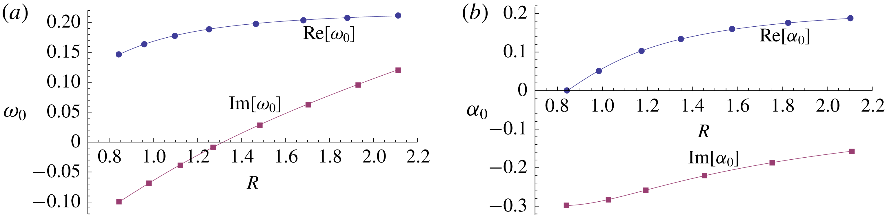
Complex frequency (a) and wavenumber (b) at the singularity as functions of the velocity ratio. Solid lines show current procedure and symbols show a few points extracted from Huerre & Monkewitz (Reference Huerre and Monkewitz1985).

The latter two can in fact be any two complex scalars, or four real scalars. For instance, one can search for the singularity
 $\text{Re}[\unicode[STIX]{x1D6FC}_{0}]$
,
 $\text{Im}[\unicode[STIX]{x1D6FC}_{0}]$
,
 $\text{Re}[\unicode[STIX]{x1D714}_{0}]$
and
 $\text{Im}[\unicode[STIX]{x1D714}_{0}]$
for a prescribed value of
 $R$
. Figure 2 presents a comparison between these singularities calculated with the present methodology and the ones obtained by Huerre & Monkewitz (Reference Huerre and Monkewitz1985) using path
 $\text{C}_{2}$
in figure 1, which were extracted from figures 5 and 6 of their paper. An excellent agreement can be observed. One can also search for the parametric condition
 $R_{0}$
at the linear onset of absolute instability instead by prescribing
 $\text{Im}[\unicode[STIX]{x1D714}_{0}]=0$
and calculating
 $\text{Re}[\unicode[STIX]{x1D6FC}_{0}]$
,
 $\text{Im}[\unicode[STIX]{x1D6FC}_{0}]$
,
 $\text{Re}[\unicode[STIX]{x1D714}_{0}]$
and
 $R_{0}$
. This yields
 $R_{0}=1.3156935913$
and
 $\text{Re}[\unicode[STIX]{x1D714}_{0}]=0.1921122457$
. These results have an absolute error of
 $O(10^{-10})$
and agree well with the values
 $R_{0}=1.315$
and
 $\text{Re}[\unicode[STIX]{x1D714}_{0}]=0.192$
reported by Huerre & Monkewitz (Reference Huerre and Monkewitz1985).
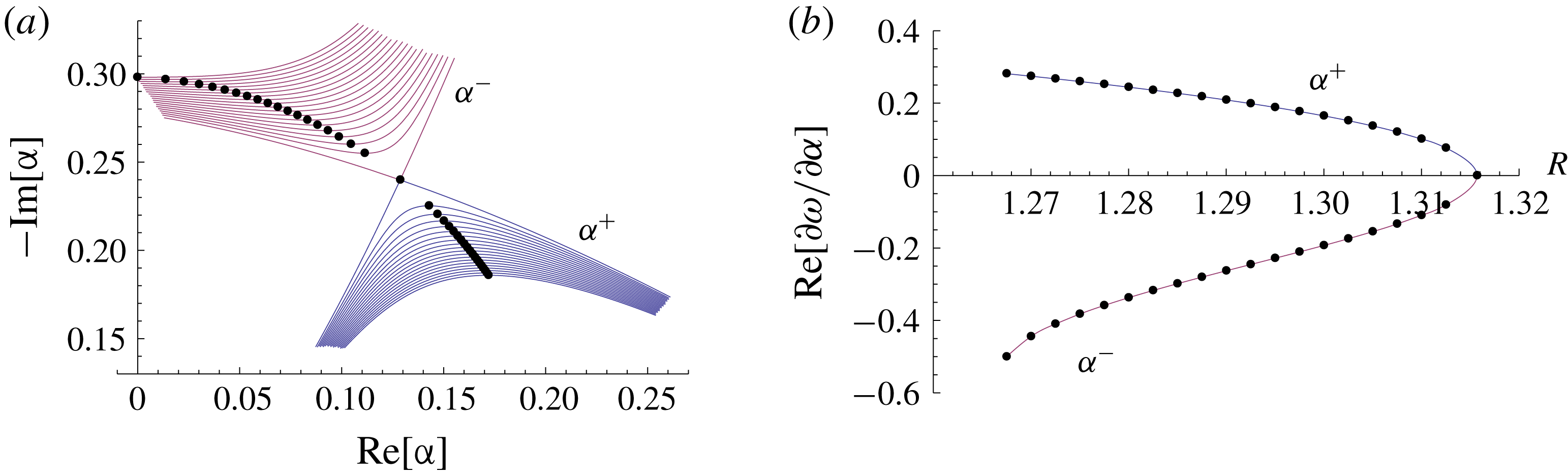
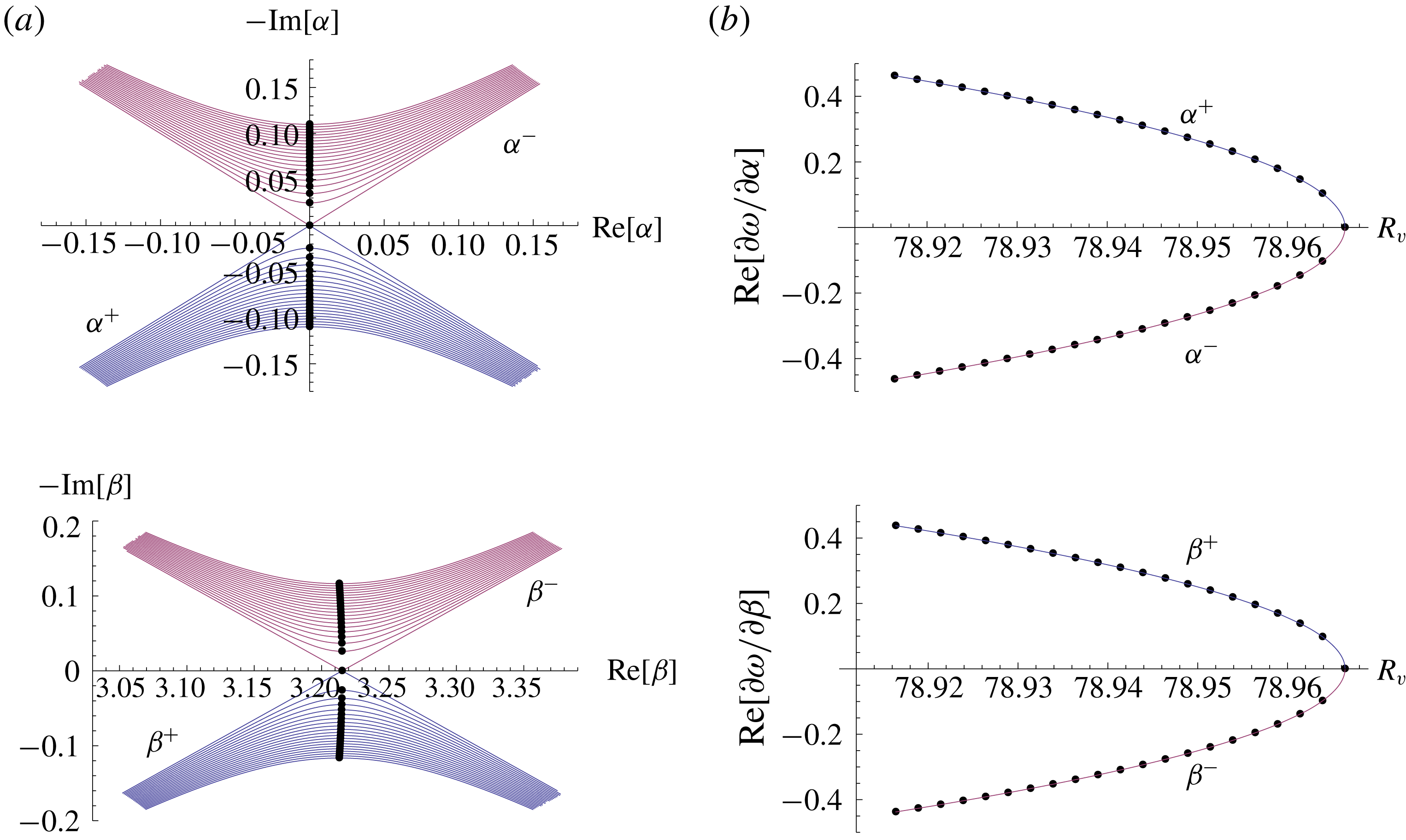
Complex streamwise wavenumber plane (a) and real group velocity (b) as functions of the velocity ratio for the planar mixing layer. Symbols in both plots represent the same modes at their respective velocity ratios.

Although this verification confirms that these singularities satisfy causality, a collision check is also performed and shown in figure 3(a). The symbols on each spatial branch involved in the collision indicate the location of the modes with a real group velocity, which is shown in figure 3(b) as functions of
 $R$
. Here
 $\text{Re}[\unicode[STIX]{x1D6FC}]$
,
 $\text{Im}[\unicode[STIX]{x1D6FC}]$
,
 $\text{Re}[\unicode[STIX]{x1D714}]$
and
 $\text{Re}[\unicode[STIX]{x2202}\unicode[STIX]{x1D714}/\unicode[STIX]{x2202}\unicode[STIX]{x1D6FC}]$
are the four scalars searched for using this methodology, while imposing
 $\text{Im}[\unicode[STIX]{x1D714}]=0$
and
 $\text{Im}[\unicode[STIX]{x2202}\unicode[STIX]{x1D714}/\unicode[STIX]{x2202}\unicode[STIX]{x1D6FC}]=0$
as well as prescribing
 $R$
. There are no more modes with these characteristics beyond the singularity, since
 $\text{Im}[\unicode[STIX]{x1D714}]=0$
is no longer true but
 $\text{Im}[\unicode[STIX]{x1D714}]>0$
instead. This plot clearly demonstrates that the colliding modes in these spatial branches do propagate in opposite directions before the singularity is reached, which is actually true for all modes in these branches.
Finally, it is possible to re-write (3.2) in the form of (2.20) with
 $s=0$
using operator
 ${\mathcal{P}}=-1/(\unicode[STIX]{x1D714}-\unicode[STIX]{x1D6FC}U_{b})^{2}$
, which satisfies the symmetry condition
 ${\mathcal{P}}{\mathcal{L}}=({\mathcal{P}}{\mathcal{L}})^{\text{T}}$
. Hence, the solvability condition defined in (2.18) for this problem becomes
 $$\begin{eqnarray}\displaystyle \int _{-\infty }^{+\infty }\left\{\frac{2\unicode[STIX]{x1D6FC}P_{n}^{2}}{(\unicode[STIX]{x1D714}-\unicode[STIX]{x1D6FC}U_{b})^{2}}-\left(\unicode[STIX]{x1D714}-\unicode[STIX]{x1D6FC}\frac{\unicode[STIX]{x2202}\unicode[STIX]{x1D714}}{\unicode[STIX]{x2202}\unicode[STIX]{x1D6FC}}\right)\frac{2(DU_{b})P_{n}(DP_{n})}{(\unicode[STIX]{x1D714}-\unicode[STIX]{x1D6FC}U_{b})^{4}}\right\}\,\text{d}z=0. & & \displaystyle\end{eqnarray}$$
Re-writing (3.8) to calculate the group velocity at
 $R=1$
, according to (2.21), yields a value of
 $O(10^{-10})$
, which is the same order of magnitude as the eigenvalue absolute error, confirming that the singularity calculated at
 $R=1$
is indeed correct.
3.2 Pseudo-two-dimensional singularities
The second test case reproduces the pseudo-two-dimensional (
 $\text{Re}[\unicode[STIX]{x1D6FD}]\neq 0$
but
 $\text{Im}[\unicode[STIX]{x1D6FD}]=0$
) absolute instability for a rotating disk from Lingwood (Reference Lingwood1995). This is the boundary layer flow formed on top of an infinitely wide disk as it rotates. The base state feeding the linear instability has two approximately parallel velocity components. It is an inflectional three-dimensional boundary layer, which is susceptible to an inviscid cross-flow instability, similar to a swept wing. Convective instability occurs near the centreline whereas absolute instability occurs sufficiently far from it. This local base state is defined on a semi-infinite domain and obtained from the boundary layer equations
 $$\begin{eqnarray}\displaystyle \left.\begin{array}{@{}c@{}}DP_{b}+W_{b}DW_{b}-D^{2}W_{b}=0\quad \text{and}\quad 2U_{b}V_{b}+W_{b}DV_{b}-DV_{b}=0,\\ U_{b}^{2}+DU_{b}W_{b}-V_{b}^{2}-D^{2}U_{b}=0,\quad 2U_{b}+DW_{b}=0,\end{array}\right\} & & \displaystyle\end{eqnarray}$$
for the streamwise, spanwise and transverse velocity components
 $U_{b}(z)$
,
 $V_{b}(z)$
and
 $W_{b}(z)$
, respectively, as well as pressure
 $P_{b}(z)$
, discussed in Schlichting (Reference Schlichting1986) and subject to boundary conditions
 $$\begin{eqnarray}\displaystyle U_{b}(0)=W_{b}(0)=P_{b}(0)=0,\quad V_{b}(0)=1\quad \text{and}\quad U_{b}(\infty )=V_{b}(\infty )=0, & & \displaystyle\end{eqnarray}$$
where the Reynolds number
 $Re$
is a control parameter built into the dimensionless variables. The direct differential eigenvalue problem, written in the form of (2.3) for the linear, modal and inviscid vertical velocity eigenfunction
 $w_{n}(z)$
, is given by
 $$\begin{eqnarray}\displaystyle {\mathcal{L}}w_{n}=0\quad \text{with}~{\mathcal{L}}=(\unicode[STIX]{x1D6FC}U_{b}+\bar{\unicode[STIX]{x1D6FD}}V_{b}-\unicode[STIX]{x1D714})(D^{2}-k^{2})-(\unicode[STIX]{x1D6FC}D^{2}U_{b}+\bar{\unicode[STIX]{x1D6FD}}D^{2}V_{b}), & & \displaystyle\end{eqnarray}$$
where
 $k^{2}=\unicode[STIX]{x1D6FC}^{2}+\bar{\unicode[STIX]{x1D6FD}}^{2}$
and
 $\bar{\unicode[STIX]{x1D6FD}}=\unicode[STIX]{x1D6FD}/Re$
is the normalised pseudo spanwise wavenumber, which acts as the sole control parameter. It is subject to boundary conditions
 $$\begin{eqnarray}\displaystyle w_{n}(z=0)=0\quad \text{and}\quad w_{n}(z\rightarrow \infty )=c_{2}\text{e}^{-\sqrt{\unicode[STIX]{x1D6FC}^{2}+\bar{\unicode[STIX]{x1D6FD}}^{2}}z}, & & \displaystyle\end{eqnarray}$$
where (3.11) is marched from infinity to the disk wall using initial conditions obtained from the right boundary condition in (3.12). In numerical terms, infinity is a high enough value of
 $z$
where the base state second derivatives are negligible. The Newton-type root-finding method can then be used to find a solution that satisfies
 $$\begin{eqnarray}\displaystyle f_{n}(\unicode[STIX]{x1D6FC},\unicode[STIX]{x1D714})=\tilde{w}_{n}(z=0)=0, & & \displaystyle\end{eqnarray}$$
which is the normalised version of the left boundary condition in (3.12) for the normalised disturbance
 $\tilde{w}_{n}(z)=w_{n}(z)/c_{2}$
, avoiding the need to find constant
 $c_{2}$
.
Taking the derivative of (3.11) with respect to
 $\unicode[STIX]{x1D6FC}$
, while noting that
 $\unicode[STIX]{x2202}U_{b}/\unicode[STIX]{x2202}\unicode[STIX]{x1D6FC}=0$
,
 $\unicode[STIX]{x2202}V_{b}/\unicode[STIX]{x2202}\unicode[STIX]{x1D6FC}=0$
and
 $\unicode[STIX]{x2202}\bar{\unicode[STIX]{x1D6FD}}/\unicode[STIX]{x2202}\unicode[STIX]{x1D6FC}=0$
, leads to the auxiliary differential eigenvalue problem
 $$\begin{eqnarray}\displaystyle & {\mathcal{L}}w_{\unicode[STIX]{x1D6FC}}={\mathcal{S}}_{\unicode[STIX]{x1D6FC}}=-{\mathcal{L}}_{\unicode[STIX]{x1D6FC}}w_{n}\quad \text{with} & \displaystyle \nonumber\\ \displaystyle & \displaystyle {\mathcal{L}}_{\unicode[STIX]{x1D6FC}}=k^{2}\frac{\unicode[STIX]{x2202}\unicode[STIX]{x1D714}}{\unicode[STIX]{x2202}\unicode[STIX]{x1D6FC}}+2\unicode[STIX]{x1D6FC}\unicode[STIX]{x1D714}-(3\unicode[STIX]{x1D6FC}^{2}+\bar{\unicode[STIX]{x1D6FD}}^{2})U_{b}-D^{2}U_{b}-2\unicode[STIX]{x1D6FC}\bar{\unicode[STIX]{x1D6FD}}V_{b}-\left(\frac{\unicode[STIX]{x2202}\unicode[STIX]{x1D714}}{\unicode[STIX]{x2202}\unicode[STIX]{x1D6FC}}-U_{b}\right)D^{2}, & \displaystyle\end{eqnarray}$$
where
 $w_{\unicode[STIX]{x1D6FC}}(z)=\unicode[STIX]{x2202}w_{n}/\unicode[STIX]{x2202}\unicode[STIX]{x1D6FC}$
is defined as an additional eigenfunction. This equation is subject to boundary conditions
 $$\begin{eqnarray}\displaystyle w_{\unicode[STIX]{x1D6FC}}(z=0)=0 & & \displaystyle\end{eqnarray}$$
and
 $$\begin{eqnarray}\displaystyle w_{\unicode[STIX]{x1D6FC}}(z\rightarrow \infty )=\left(c_{4}-\unicode[STIX]{x1D6FC}c_{2}\left(\frac{1}{2\left(\unicode[STIX]{x1D6FC}^{2}+\bar{\unicode[STIX]{x1D6FD}}^{2}\right)}+\frac{z}{\sqrt{\unicode[STIX]{x1D6FC}^{2}+\bar{\unicode[STIX]{x1D6FD}}^{2}}}\right)\right)\text{e}^{-\sqrt{\unicode[STIX]{x1D6FC}^{2}+\bar{\unicode[STIX]{x1D6FD}}^{2}}z}, & & \displaystyle\end{eqnarray}$$
which can be further simplified by choosing
 $c_{4}=\unicode[STIX]{x1D6FC}c_{2}/(2(\unicode[STIX]{x1D6FC}^{2}+\bar{\unicode[STIX]{x1D6FD}}^{2}))$
, yielding the same boundary conditions one would obtain by taking the derivative of (3.11) with respect to
 $\unicode[STIX]{x1D6FC}$
while neglecting the dependence of
 $c_{2}$
on
 $\unicode[STIX]{x1D6FC}$
. Once again, this is possible because (3.14) and (3.15) are also an eigenvalue problem, which is undetermined up to a constant. The Newton-type method now finds a solution that satisfies (3.13) and
 $$\begin{eqnarray}\displaystyle f_{\unicode[STIX]{x1D6FC}}(\unicode[STIX]{x1D6FC},\unicode[STIX]{x1D714})=\bar{w}_{\unicode[STIX]{x1D6FC}}(z=0)=0, & & \displaystyle\end{eqnarray}$$
which is the normalised left boundary condition in (3.15) for the normalised disturbance
 $\bar{w}_{\unicode[STIX]{x1D6FC}}(z)=w_{\unicode[STIX]{x1D6FC}}(z)/c_{2}$
. This shooting method produces the two complex eigenfunctions
 $\bar{w}_{n}(z)$
and
 $\bar{w}_{\unicode[STIX]{x1D6FC}}(z)$
as well as two complex eigenvalues, or four arbitrary real scalars.
Selecting
 $\text{Re}[\unicode[STIX]{x1D6FC}_{0}]$
,
 $\text{Im}[\unicode[STIX]{x1D6FC}_{0}]$
,
 $\text{Re}[\unicode[STIX]{x1D714}_{0}]$
and
 $\text{Im}[\unicode[STIX]{x1D714}_{0}]$
as the four scalars enables this methodology to search for singularities at prescribed values of
 $\bar{\unicode[STIX]{x1D6FD}}$
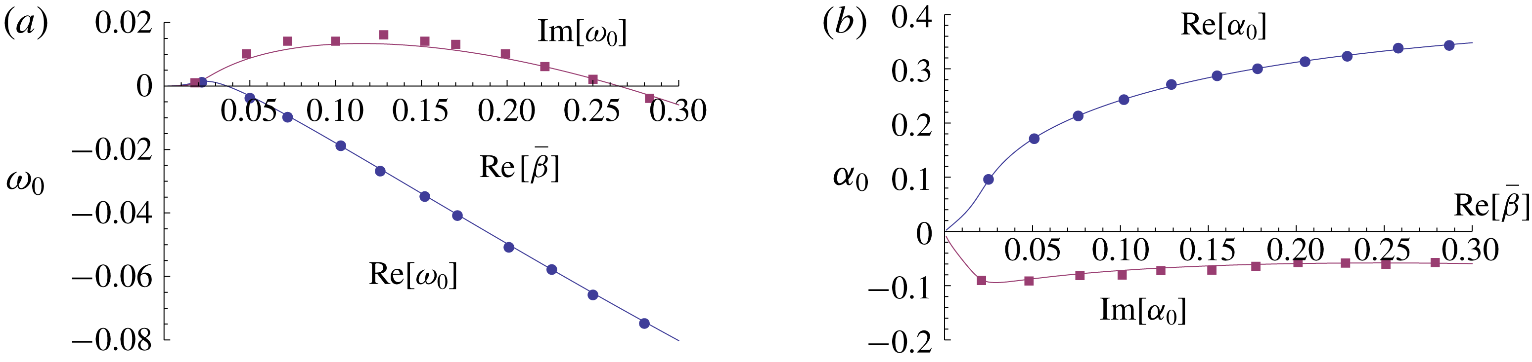
. Figure 4 compares them with the ones obtained by Lingwood (Reference Lingwood1995) using path
 $\text{C}_{2}$
in figure 1, which were extracted from figure 4 of their paper. The agreement is good in most cases but less so for
 $\text{Im}[\unicode[STIX]{x1D714}_{0}]$
, which is most likely due to the poor quality of the scanned paper available online. This can be confirmed by a quantitative comparison of the singularity at
 $\bar{\unicode[STIX]{x1D6FD}}_{0}=0.126$
, which yields
 $\unicode[STIX]{x1D714}_{0}=-0.0261664452+0.0133000530\text{i}$
and
 $\unicode[STIX]{x1D6FC}_{0}=0.2655922101-0.0669389400\text{i}$
with an absolute error of
 $O(10^{-11})$
. These numbers agree well with the results
 $\unicode[STIX]{x1D714}_{0}=-0.0262+0.0133\text{i}$
and
 $\unicode[STIX]{x1D6FC}_{0}=0.266-0.0670\text{i}$
reported by Lingwood (Reference Lingwood1995). Imposing
 $\text{Im}[\unicode[STIX]{x1D714}_{0}]=0$
and searching for
 $\bar{\unicode[STIX]{x1D6FD}}$
instead reveals that the onset of absolute instability occurs at
 $\bar{\unicode[STIX]{x1D6FD}}_{0}=0.26514812331$
,
 $\text{Re}[\unicode[STIX]{x1D714}_{0}]=-0.06982182860$
and
 $\unicode[STIX]{x1D6FC}_{0}=0.33786742527-0.05817350830\text{i}$
with the same absolute error. These numbers agree well with the values
 $\bar{\unicode[STIX]{x1D6FD}}_{0}=0.265$
,
 $\text{Re}[\unicode[STIX]{x1D714}_{0}]=-0.0698$
and
 $\unicode[STIX]{x1D6FC}_{0}=0.338-0.0582\text{i}$
, also reported by Lingwood (Reference Lingwood1995).
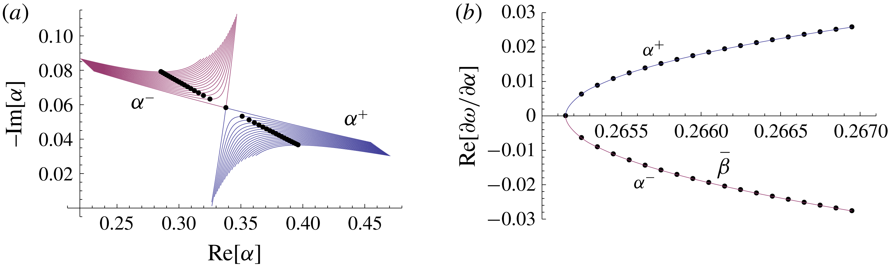
Complex frequency (a) and wavenumber (b) at the singularity as functions of the modified spanwise wavenumber. Solid lines show current procedure and symbols show a few points extracted from Lingwood (Reference Lingwood1995).

Complex streamwise wavenumber plane (a) and real group velocity (b) as functions of the normalised spanwise wavenumber for the rotating disk. Symbols in both plots represent the same modes at their respective normalised spanwise wavenumber.

Once again, it is important to verify the collision criterion in order to demonstrate causality and show its relation to the group velocity. Figure 5(a) shows the collision check within the convectively unstable region up to the onset of absolute instability, where the symbols indicate the location of the mode with a real group velocity on each spatial branch involved in the collision. These same symbols are also shown in figure 5(b), which presents their real group velocity as a function of the normalised spanwise wavenumber. They were calculated by selecting
 $\text{Re}[\unicode[STIX]{x1D6FC}]$
,
 $\text{Im}[\unicode[STIX]{x1D6FC}]$
,
 $\text{Re}[\unicode[STIX]{x1D714}]$
and
 $\text{Re}[\unicode[STIX]{x2202}\unicode[STIX]{x1D714}/\unicode[STIX]{x2202}\unicode[STIX]{x1D6FC}]$
as the four scalars searched for using this methodology, while imposing
 $\text{Im}[\unicode[STIX]{x1D714}]=0$
and
 $\text{Im}[\unicode[STIX]{x2202}\unicode[STIX]{x1D714}/\unicode[STIX]{x2202}\unicode[STIX]{x1D6FC}]=0$
as well as prescribing
 $\bar{\unicode[STIX]{x1D6FD}}$
. This is the reason why no more modes with these characteristics can be included beyond the singularity, since
 $\text{Im}[\unicode[STIX]{x1D714}]=0$
is no longer true but
 $\text{Im}[\unicode[STIX]{x1D714}]>0$
instead. Once again, these modes in their respective colliding spatial branches do propagate in opposite directions before the singularity is reached.
Finally, it is possible to re-write (3.11) in the form of (2.20) with
 $s=0$
using operator
 ${\mathcal{P}}=1/(\unicode[STIX]{x1D714}-\unicode[STIX]{x1D6FC}U_{b}-\bar{\unicode[STIX]{x1D6FD}}V_{b})$
, which satisfies the symmetry condition
 ${\mathcal{P}}{\mathcal{L}}=({\mathcal{P}}{\mathcal{L}})^{\text{T}}$
. Hence, the solvability condition in (2.18) for this problem becomes
 $$\begin{eqnarray}\displaystyle & & \displaystyle \int _{0}^{\infty }\left\{\left(\frac{\unicode[STIX]{x2202}\unicode[STIX]{x1D714}}{\unicode[STIX]{x2202}\unicode[STIX]{x1D6FC}}-U_{b}\right)\frac{w_{n}D^{2}w_{n}}{\unicode[STIX]{x1D714}-\unicode[STIX]{x1D6FC}U_{b}-\bar{\unicode[STIX]{x1D6FD}}V_{b}}\right.\nonumber\\ \displaystyle & & \displaystyle \quad \left.-\left(k^{2}\frac{\unicode[STIX]{x2202}\unicode[STIX]{x1D714}}{\unicode[STIX]{x2202}\unicode[STIX]{x1D6FC}}+2\unicode[STIX]{x1D6FC}\unicode[STIX]{x1D714}-(3\unicode[STIX]{x1D6FC}^{2}+\bar{\unicode[STIX]{x1D6FD}}^{2})U_{b}-D^{2}U_{b}-2\unicode[STIX]{x1D6FC}\bar{\unicode[STIX]{x1D6FD}}V_{b}\right)\frac{w_{n}^{2}}{\unicode[STIX]{x1D714}-\unicode[STIX]{x1D6FC}U_{b}-\bar{\unicode[STIX]{x1D6FD}}V_{b}}\right\}\,\text{d}z=0.\nonumber\\ \displaystyle & & \displaystyle\end{eqnarray}$$
Following (2.21), the group velocity at
 $\bar{\unicode[STIX]{x1D6FD}}=0.126$
is extracted from (3.17) to yield a value of
 $O(10^{-6})$
, which is five orders of magnitude higher than the eigenvalue absolute error. This integrand decays slowly and, hence, its non-negligible contributions extend far into the
 $z$
domain. Errors accumulate because it becomes increasingly difficult to generate accurate base flow solutions for such large
 $z$
values.
3.3 Three-dimensional singularities
The third test case is the three-dimensional (
 $\unicode[STIX]{x1D6FC}\neq 0$
and
 $\unicode[STIX]{x1D6FD}\neq 0$
) absolute instability of the heated flow in a saturated homogeneous porous medium reported by Brevdo (Reference Brevdo2009). This is the flow generated by an inclined temperature gradient and a vertical throughflow. The base state has a non-parallel but still local two-component velocity field and a non-local two-dimensional temperature profile. This forced base flow convection can be superposed on natural convection due to buoyancy driven instabilities, which can be either convective or absolute, depending on a non-trivial combination of the three governing parameter values. Its local base state is given by
 $$\begin{eqnarray}\displaystyle \left.\begin{array}{@{}c@{}}U_{b}(z)=R_{h}z,\quad V_{b}(z)=0,\quad W_{b}(z)=Q_{v}\quad \text{and}\\ \displaystyle T_{b}(z)=\frac{R_{h}^{2}}{2Q_{v}}\left(z^{2}+\frac{2z}{Q_{v}}-\frac{1}{4}\right)-\frac{Q_{v}^{2}R_{v}+R_{h}^{2}}{2Q_{v}^{2}\sinh [Q_{v}/2]}(\text{e}^{Q_{v}z}-\cosh [Q_{v}/2])-R_{h}x,\end{array}\right\} & & \displaystyle\end{eqnarray}$$
for the streamwise, spanwise and transverse velocity components
 $U_{b}(z)$
,
 $V_{b}(z)$
and
 $W_{b}(z)$
, respectively, as well as temperature
 $T_{b}(z)$
, defined on the finite domain
 $-1/2\leqslant z\leqslant +1/2$
.
 $R_{v}$
,
 $R_{h}$
and
 $Q_{v}$
are the vertical and horizontal Rayleigh numbers and Péclet number, respectively. The direct differential eigenvalue problem, written in the form of (2.3) for the linear and modal transverse velocity eigenfunction
 $w_{n}(z)$
, is given by
 $$\begin{eqnarray}\displaystyle {\mathcal{L}}w_{n}=0\quad \text{with}~{\mathcal{L}} & = & \displaystyle D^{4}-Q_{v}D^{3}-(2k^{2}-\text{i}(\unicode[STIX]{x1D714}-\unicode[STIX]{x1D6FC}U_{b}))D^{2}+(Q_{v}k^{2}-\text{i}\unicode[STIX]{x1D6FC}R_{h})D\nonumber\\ \displaystyle & & \displaystyle +\,k^{2}(k^{2}-\text{i}(\unicode[STIX]{x1D714}-\unicode[STIX]{x1D6FC}U_{b})+DT_{b}),\end{eqnarray}$$
where
 $k^{2}=\unicode[STIX]{x1D6FC}^{2}+\unicode[STIX]{x1D6FD}^{2}$
and the
 $x$
dependence of the base flow temperature is omitted, i.e.
 $T_{b}(z)$
is used instead of
 $T_{b}(x,z)$
, since only a derivative of
 $T_{b}$
with respect to
 $z$
appears in (3.19). This equation is subject to boundary conditions
 $$\begin{eqnarray}\displaystyle w_{n}(z=\pm 1/2)=D^{2}w_{n}(z=\pm 1/2)=0, & & \displaystyle\end{eqnarray}$$
and marched from
 $z=-1/2$
to
 $+1/2$
using as initial conditions the boundary conditions at
 $z=-1/2$
in (3.20), in addition to
 $$\begin{eqnarray}\displaystyle Dw_{n}(z=-1/2)=c_{1}\quad \text{and}\quad D^{3}w_{n}(z=-1/2)=c_{2}, & & \displaystyle\end{eqnarray}$$
where
 $c_{1}$
and
 $c_{2}$
are unknown complex constants. The Newton-type root-finding method can then be used to find a solution that satisfies
 $$\begin{eqnarray}\displaystyle f_{n}(\unicode[STIX]{x1D6FC},\unicode[STIX]{x1D6FD},\unicode[STIX]{x1D714})=\{\tilde{w}_{n}(z=+/2),D^{2}\tilde{w}_{n}(z=+1/2)\}=0, & & \displaystyle\end{eqnarray}$$
which is the normalised version of the boundary conditions at
 $z=+1/2$
in (3.20) for the normalised disturbance
 $\tilde{w}_{n}(z)=w_{n}(z)/c_{2}$
, avoiding the need to find constant
 $c_{2}$
. Contrary to the previous two test cases,
 $f_{n}(\unicode[STIX]{x1D6FC},\unicode[STIX]{x1D6FD},\unicode[STIX]{x1D714})=0$
represents two complex equations for a single complex eigenvector, namely
 $w_{n}(z)$
, but two complex eigenvalues. In this particular case,
 $c_{1}$
is also an eigenvalue and it must be obtained. Hence, this allows the search for only one physically meaningful complex eigenvalue, or two real scalars.
Taking the derivative of (3.19) with respect to
 $\unicode[STIX]{x1D6FC}$
, while noting that
 $\unicode[STIX]{x2202}U_{b}/\unicode[STIX]{x2202}\unicode[STIX]{x1D6FC}=\unicode[STIX]{x2202}T_{b}/\unicode[STIX]{x2202}\unicode[STIX]{x1D6FC}=0$
and
 $\unicode[STIX]{x2202}R_{h}/\unicode[STIX]{x2202}\unicode[STIX]{x1D6FC}=\unicode[STIX]{x2202}R_{v}/\unicode[STIX]{x2202}\unicode[STIX]{x1D6FC}=\unicode[STIX]{x2202}Q_{v}/\unicode[STIX]{x2202}\unicode[STIX]{x1D6FC}=0$
, leads to the auxiliary problem
 $$\begin{eqnarray}\displaystyle & {\mathcal{L}}w_{\unicode[STIX]{x1D6FC}}={\mathcal{S}}_{\unicode[STIX]{x1D6FC}}=-{\mathcal{L}}_{\unicode[STIX]{x1D6FC}}w_{n}\quad \text{with} & \displaystyle \nonumber\\ \displaystyle & \displaystyle {\mathcal{L}}_{\unicode[STIX]{x1D6FC}}=2\unicode[STIX]{x1D6FC}(2k^{2}-\text{i}(\unicode[STIX]{x1D714}-\unicode[STIX]{x1D6FC}U_{b})+DT_{b})-\text{i}k^{2}\left(\frac{\text{d}\unicode[STIX]{x1D714}}{\text{d}\unicode[STIX]{x1D6FC}}-U_{b}\right) & \displaystyle \nonumber\\ \displaystyle & \displaystyle \quad +\,(2Q_{v}\unicode[STIX]{x1D6FC}-\text{i}R_{h})D-\left(4\unicode[STIX]{x1D6FC}-\text{i}\left(\frac{\text{d}\unicode[STIX]{x1D714}}{\text{d}\unicode[STIX]{x1D6FC}}-U_{b}\right)\right)D^{2}, & \displaystyle\end{eqnarray}$$
where
 $w_{\unicode[STIX]{x1D6FC}}(z)=\unicode[STIX]{x2202}w_{n}/\unicode[STIX]{x2202}\unicode[STIX]{x1D6FC}$
is defined as an additional eigenfunction. This equation is subject to boundary conditions
 $$\begin{eqnarray}\displaystyle w_{\unicode[STIX]{x1D6FC}}(z=\pm 1/2)=D^{2}w_{\unicode[STIX]{x1D6FC}}(z=\pm 1/2)=0, & & \displaystyle\end{eqnarray}$$
obtained by taking the derivative of (3.20) with respect to
 $\unicode[STIX]{x1D6FC}$
. In order to transform (3.23) to (3.24) into an initial value problem, the additional initial conditions
 $$\begin{eqnarray}\displaystyle Dw_{\unicode[STIX]{x1D6FC}}(z=-1/2)=c_{3}\quad \text{and}\quad D^{3}w_{\unicode[STIX]{x1D6FC}}(z=-1/2)=c_{4}, & & \displaystyle\end{eqnarray}$$
are employed, as done with (3.21), where
 $c_{3}$
and
 $c_{4}$
are unknown complex constants. The root-finding method employed previously now must solve (3.22) and
 $$\begin{eqnarray}\displaystyle f_{\unicode[STIX]{x1D6FC}}(\unicode[STIX]{x1D6FC},\unicode[STIX]{x1D6FD},\unicode[STIX]{x1D714})=\{\tilde{w}_{\unicode[STIX]{x1D6FC}}(z=+/2),D^{2}\tilde{w}_{\unicode[STIX]{x1D6FC}}(z=+1/2)\}=0, & & \displaystyle\end{eqnarray}$$
which is the normalised version of the boundary conditions at
 $z=+1/2$
in (3.24) for the normalised disturbance
 $\tilde{w}_{\unicode[STIX]{x1D6FC}}(z)=w_{\unicode[STIX]{x1D6FC}}(z)/c_{4}$
, avoiding the need to find constant
 $c_{4}$
. Equations (3.22) and (3.26) yield four complex equations for two complex eigenvectors, namely
 $w_{n}(z)$
and
 $w_{\unicode[STIX]{x1D6FC}}(z)$
, as well as four complex eigenvalues. Now,
 $c_{1}$
and
 $c_{3}$
are also eigenvalues and must be obtained. Hence, this allows the search for two physically meaningful complex eigenvalues, or four real scalars.
Up to this point, one can use the above equations to solve either a two-dimensional or a pseudo-two-dimensional linear and local stability problem by prescribing
 $\unicode[STIX]{x1D6FD}=0$
or
 $\text{Re}[\unicode[STIX]{x1D6FD}]\neq 0$
and
 $\text{Im}[\unicode[STIX]{x1D6FD}]=0$
, respectively. In order to solve a three-dimensional stability problem instead, the value of
 $\unicode[STIX]{x1D6FD}$
must not be prescribed a priori but obtained as a solution as well. Hence, an additional auxiliary equation is required. Taking the derivative of (3.19) with respect to
 $\unicode[STIX]{x1D6FD}$
, while noting that
 $\unicode[STIX]{x2202}U_{b}/\unicode[STIX]{x2202}\unicode[STIX]{x1D6FD}=\unicode[STIX]{x2202}T_{b}/\unicode[STIX]{x2202}\unicode[STIX]{x1D6FD}=0$
and
 $\unicode[STIX]{x2202}R_{h}/\unicode[STIX]{x2202}\unicode[STIX]{x1D6FD}=\unicode[STIX]{x2202}R_{v}/\unicode[STIX]{x2202}\unicode[STIX]{x1D6FD}=\unicode[STIX]{x2202}Q_{v}/\unicode[STIX]{x2202}\unicode[STIX]{x1D6FD}=0$
, leads to additional auxiliary differential eigenvalue problem
 $$\begin{eqnarray}\displaystyle & {\mathcal{L}}w_{\unicode[STIX]{x1D6FD}}={\mathcal{S}}_{\unicode[STIX]{x1D6FD}}=-{\mathcal{L}}_{\unicode[STIX]{x1D6FD}}w_{n}\quad \text{with} & \displaystyle \nonumber\\ \displaystyle & \displaystyle {\mathcal{L}}_{\unicode[STIX]{x1D6FD}}=2\unicode[STIX]{x1D6FD}(2k^{2}-\text{i}(\unicode[STIX]{x1D714}-\unicode[STIX]{x1D6FC}U_{b})+DT_{b})-\text{i}k^{2}\frac{\text{d}\unicode[STIX]{x1D714}}{\text{d}\unicode[STIX]{x1D6FD}}+2Q_{v}\unicode[STIX]{x1D6FD}D-\left(4\unicode[STIX]{x1D6FD}-\text{i}\frac{\text{d}\unicode[STIX]{x1D714}}{\text{d}\unicode[STIX]{x1D6FD}}\right)D^{2}, & \displaystyle\end{eqnarray}$$
where
 $w_{\unicode[STIX]{x1D6FD}}(z)=\unicode[STIX]{x2202}w_{n}/\unicode[STIX]{x2202}\unicode[STIX]{x1D6FD}$
is defined as an additional eigenfunction. This equation is subject to boundary conditions
 $$\begin{eqnarray}\displaystyle w_{\unicode[STIX]{x1D6FD}}(z=\pm 1/2)=D^{2}w_{\unicode[STIX]{x1D6FD}}(z=\pm 1/2)=0, & & \displaystyle\end{eqnarray}$$
obtained by taking the derivative of (3.20) with respect to
 $\unicode[STIX]{x1D6FD}$
. In order to transform (3.27) to (3.28) into an initial value problem, the additional initial conditions
 $$\begin{eqnarray}\displaystyle Dw_{\unicode[STIX]{x1D6FD}}(z=-1/2)=c_{5}\quad \text{and}\quad D^{3}w_{\unicode[STIX]{x1D6FD}}(z=-1/2)=c_{6}, & & \displaystyle\end{eqnarray}$$
are employed, as done with (3.21) and (3.25), where
 $c_{5}$
and
 $c_{6}$
are unknown complex constants. The root-finding method is now adapted to solve (3.22), (3.26) and
 $$\begin{eqnarray}\displaystyle f_{\unicode[STIX]{x1D6FD}}(\unicode[STIX]{x1D6FC},\unicode[STIX]{x1D6FD},\unicode[STIX]{x1D714})=\{\tilde{w}_{\unicode[STIX]{x1D6FC}}(z=+/2),D^{2}\tilde{w}_{\unicode[STIX]{x1D6FD}}(z=+1/2)\}=0, & & \displaystyle\end{eqnarray}$$
which is the normalised version of the boundary conditions at
 $z=+1/2$
in (3.28) for the normalised disturbance
 $\tilde{w}_{\unicode[STIX]{x1D6FD}}(z)=w_{\unicode[STIX]{x1D6FD}}(z)/c_{6}$
, avoiding the need to find constant
 $c_{6}$
. Equations (3.22), (3.26) and (3.30) represent six complex equations for three complex eigenvectors, namely
 $w_{n}(z)$
,
 $w_{\unicode[STIX]{x1D6FC}}(z)$
and
 $w_{\unicode[STIX]{x1D6FD}}(z)$
, as well as six complex eigenvalues. In this case,
 $c_{1}$
,
 $c_{3}$
and
 $c_{5}$
are also eigenvalues that must be obtained. Hence, this allows the search for three physically meaningful complex eigenvalues, or six real scalars.
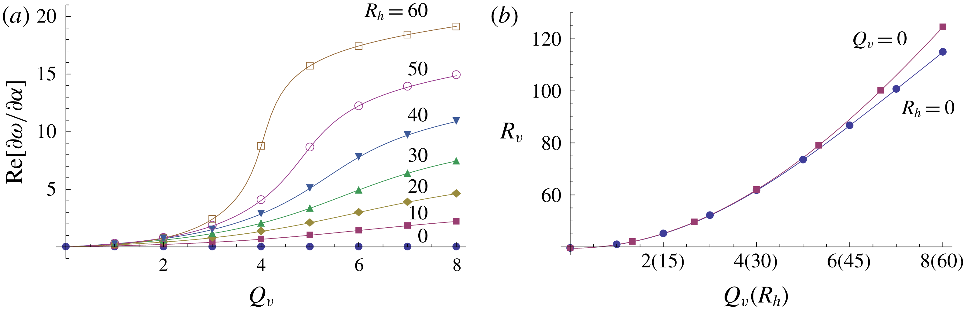
Figure 6 presents results at the onset of convective instability obtained by the current procedure for different values of the Péclet and horizontal Rayleigh numbers, comparing them with the results in tables 1 and 3 from Brevdo (Reference Brevdo2009). Solid lines represent real group velocities (a) and critical vertical Rayleigh numbers (b). The former was obtained by selecting
 $\text{Re}[\unicode[STIX]{x1D6FC}]$
,
 $\text{Re}[\unicode[STIX]{x1D6FD}]$
,
 $\text{Re}[\unicode[STIX]{x1D714}]$
,
 $R_{v}$
,
 $\text{Re}[\unicode[STIX]{x2202}\unicode[STIX]{x1D714}/\unicode[STIX]{x2202}\unicode[STIX]{x1D6FC}]$
and
 $\text{Re}[\unicode[STIX]{x2202}\unicode[STIX]{x1D714}/\unicode[STIX]{x2202}\unicode[STIX]{x1D6FD}]$
as the six real scalars provided by the method while imposing
 $\text{Im}[\unicode[STIX]{x1D6FC}]=\text{Im}[\unicode[STIX]{x1D6FD}]=\text{Im}[\unicode[STIX]{x1D714}]=0$
and
 $\text{Im}[\unicode[STIX]{x2202}\unicode[STIX]{x1D714}/\unicode[STIX]{x2202}\unicode[STIX]{x1D6FC}]=\text{Im}[\unicode[STIX]{x2202}\unicode[STIX]{x1D714}/\unicode[STIX]{x2202}\unicode[STIX]{x1D6FD}]=0$
for prescribed values of
 $R_{h}$
and
 $Q_{v}$
. On the other hand, the latter was obtained by selecting
 $\text{Re}[\unicode[STIX]{x1D6FC}_{0}]$
,
 $\text{Im}[\unicode[STIX]{x1D6FC}_{0}]$
,
 $\text{Re}[\unicode[STIX]{x1D6FD}_{0}]$
,
 $\text{Re}[\unicode[STIX]{x1D6FD}_{0}]$
,
 $\text{Re}[\unicode[STIX]{x1D714}]$
and
 $R_{v}$
as the six real scalars provided by the method while imposing
 $\text{Im}[\unicode[STIX]{x1D714}_{0}]=0$
and
 $\unicode[STIX]{x2202}\unicode[STIX]{x1D714}/\unicode[STIX]{x2202}\unicode[STIX]{x1D6FC}=\unicode[STIX]{x2202}\unicode[STIX]{x1D714}/\unicode[STIX]{x2202}\unicode[STIX]{x1D6FD}=0$
for prescribed values of
 $R_{h}$
and
 $Q_{v}$
. Brevdo (Reference Brevdo2009) calculates the onset of convective instability and then evaluates the group velocity at these conditions in order to check if they might represent an onset of absolute instability as well. The former figure confirms his finding that the onsets of convective and absolute instability only coincide when
 $Q_{v}R_{h}=0$
, since the group velocity only goes to zero when either
 $Q_{v}=0$
or
 $R_{h}=0$
. Critical vertical Rayleigh numbers for the onset of absolute instability at these two limiting cases are shown in figure 6(b), agreeing with his calculations regarding where the onsets of convective and absolute instability coincide. These numbers at
 $Q_{v}=8$
and
 $R_{h}=0$
as well as
 $Q_{v}=0$
and
 $R_{h}=60$
are
 $R_{h}=114.832605711515$
and
 $124.4728454361939$
, respectively obtained with as absolute error of
 $O(10^{-12})$
. They are in quantitative agreement with the values
 $R_{h}=114.84$
and
 $124.48$
reported by Brevdo (Reference Brevdo2009) at the same parametric conditions. It is worth pointing out that the current procedure was also used to calculate the two-dimensional (
 $\unicode[STIX]{x1D6FD}=0$
) onset of absolute instability for this problem. Although these results are not shown here, they agree with Brevdo & Ruderman (Reference Brevdo and Ruderman2009), showing that both convective and absolute onsets of instability coincide even when
 $Q_{v}R_{h}\neq 0$
.
Real group velocity (a) and vertical Rayleigh number (b) at the singularity as functions of the Péclet number (a,b) or horizontal Rayleigh number (b). Cases where
 $Q_{v}R_{h}=0$
satisfy causality;
 $\text{Re}[\unicode[STIX]{x2202}\unicode[STIX]{x1D714}/\unicode[STIX]{x2202}\unicode[STIX]{x1D6FD}]=0$
for all cases. Solid lines show current procedure and symbols show a few data points taken from Brevdo (Reference Brevdo2009).

In order to provide evidence that the singularities calculated satisfy causality, a collision check was performed for a few arbitrarily chosen parametric conditions. One of them, where
 $Q_{v}=0$
and
 $R_{h}=40$
, is shown in figure 7(a) as a function of
 $R_{v}$
for both streamwise (top) and transverse (bottom) complex wavenumber planes. The former is plotted at
 $\unicode[STIX]{x1D6FD}=\unicode[STIX]{x1D6FD}_{0}=3.215215718763$
whereas the latter is plotted at
 $\unicode[STIX]{x1D6FC}=\unicode[STIX]{x1D6FC}_{0}=0$
, which is the singularity for
 $R_{v}=78.96639607652$
. Once again, these results were obtained with an absolute error of
 $O(10^{-12})$
. Symbols indicate the modes within each spatial branch that have a real group velocity, which is shown in figure 7(b). Top and bottom real group velocities shown are obtained by pseudo two-dimensional calculations imposing
 $\unicode[STIX]{x1D6FD}=\unicode[STIX]{x1D6FD}_{0}$
and
 $\unicode[STIX]{x1D6FC}=\unicode[STIX]{x1D6FC}_{0}$
, respectively. Brevdo (Reference Brevdo2009) reported zero group velocities at
 $\unicode[STIX]{x1D6FC}_{0}=0$
,
 $\unicode[STIX]{x1D6FD}_{0}=3.22$
and
 $R_{v}=78.967$
, in agreement with the present results. This figure indicates a collision between branches with opposite group velocities coming from opposite sides of the complex plane for both streamwise and transverse wavenumbers, confirming that the singularity satisfies causality according to Brevdo (Reference Brevdo1991).
Complex (top) streamwise and (bottom) transverse (a) wavenumber planes as well as (top) streamwise and (bottom) transverse (b) real group velocities as functions of the vertical Rayleigh number for the porous medium problem with
 $Q_{v}=0$
and
 $R_{h}=40$
. Symbols in all plots represent the same modes at their respective vertical Rayleigh numbers.

Finally, solvability conditions are evaluated for this test case. Unfortunately, it is not possible to define an operator
 ${\mathcal{P}}$
that allows the linear and homogeneous operator in (3.19) to satisfy (2.20), i.e.
 ${\mathcal{P}}{\mathcal{L}}\neq ({\mathcal{P}}{\mathcal{L}})^{\text{T}}$
. Hence, the classical adjoint based solvability conditions defined in (2.13) and (2.14) must be used instead of (2.18) and (2.19), which are modified solvability conditions defined for symmetric operators. An adjoint problem of (3.19), based on (2.12), can be written as
 $$\begin{eqnarray}\displaystyle {\mathcal{L}}^{\ast }w_{n}^{+}=0\quad \text{with}~{\mathcal{L}}^{\ast } & = & \displaystyle D^{4}+Q_{v}D^{3}-(2\bar{k}^{2}+\text{i}(\bar{\unicode[STIX]{x1D714}}-\bar{\unicode[STIX]{x1D6FC}}U_{b}))D^{2}-(Q_{v}\bar{k}^{2}-\text{i}\bar{\unicode[STIX]{x1D6FC}}R_{h})D\nonumber\\ \displaystyle & & \displaystyle +\,\bar{k}^{2}(\bar{k}^{2}+\text{i}(\bar{\unicode[STIX]{x1D714}}-\bar{\unicode[STIX]{x1D6FC}}U_{b})+DT_{b}),\end{eqnarray}$$
when subject to boundary conditions
 $$\begin{eqnarray}\displaystyle w_{n}^{+}(z=\pm 1/2)=(D^{2}+Q_{v}D)w_{n}^{+}(z=\pm 1/2)=0, & & \displaystyle\end{eqnarray}$$
allowing
 $w_{n}^{+}$
to be an adjoint of
 $w_{n}$
. The classical solvability conditions then become
 $$\begin{eqnarray}\displaystyle & & \displaystyle \int _{-1/2}^{+1/2}\left\{\left(4\unicode[STIX]{x1D6FC}-\text{i}\left(\frac{\text{d}\unicode[STIX]{x1D714}}{\text{d}\unicode[STIX]{x1D6FC}}-U_{b}\right)\right)D^{2}w_{n}-(2Q_{v}\unicode[STIX]{x1D6FC}-\text{i}R_{h})Dw_{n}\right.\nonumber\\ \displaystyle & & \displaystyle \qquad -\left.\left(2\unicode[STIX]{x1D6FC}(2k^{2}-\text{i}(\unicode[STIX]{x1D714}-\unicode[STIX]{x1D6FC}U_{b})+DT_{b})-\text{i}k^{2}\left(\frac{\text{d}\unicode[STIX]{x1D714}}{\text{d}\unicode[STIX]{x1D6FC}}-U_{b}\right)\right)w_{n}\right\}\bar{w}_{n}^{+}\,\text{d}z=0\end{eqnarray}$$
and
 $$\begin{eqnarray}\displaystyle & & \displaystyle \int _{-1/2}^{+1/2}\left\{\left(4\unicode[STIX]{x1D6FD}-\text{i}\frac{\text{d}\unicode[STIX]{x1D714}}{\text{d}\unicode[STIX]{x1D6FD}}\right)D^{2}w_{n}-2Q_{v}\unicode[STIX]{x1D6FD}Dw_{n}\right.\nonumber\\ \displaystyle & & \displaystyle \qquad -\left.\left(2\unicode[STIX]{x1D6FD}(2k^{2}-\text{i}(\unicode[STIX]{x1D714}-\unicode[STIX]{x1D6FC}U_{b})+DT_{b})-\text{i}k^{2}\frac{\text{d}\unicode[STIX]{x1D714}}{\text{d}\unicode[STIX]{x1D6FD}}\right)w_{n}\right\}\bar{w}_{n}^{+}\,\text{d}z=0,\end{eqnarray}$$
respectively. Based on (2.15) and (2.16), the above equations can be re-written to provide formulas for their respective group velocities. They yield a value of
 $O(10^{-12})$
at
 $Q_{v}=0$
and
 $R_{h}=40$
, which is the same order of magnitude as the eigenvalue absolute error. This confirms that the singularity calculated at
 $Q_{v}=0$
and
 $R_{h}=40$
is correct and it does allow group velocity calculations for all modes in the colliding branches.
3.4 Comparative efficiency evaluation
It is important to evaluate the efficiency of the present methodology relative to the other traditional methods from the literature illustrated in figure 1. Such a comparison is very often strongly problem dependent and usually has a high degree of subjectivity, which arises from the fact that one can choose from a wide array of error tolerances, numerical schemes, software libraries, computer hardwares and so on. Hence, definitive answers are beyond the scope of this paper. It is possible, however, to provide some reasonable efficiency estimates based on different metrics. They are provided in this subsection for both two- and three-dimensional absolute instabilities found in the third test case of this paper, originally studied by Brevdo (Reference Brevdo2009).
Comparisons with path
 $\text{A}_{1}$
from figure 1 are excluded from this study. Such comparisons are not pertinent because the present methodology was developed for eigenvalue problems whose eigenfunction dependence on the single inhomogeneous coordinate cannot be written in a simple analytical form. In other words, the present methodology was developed for differential eigenvalue problems. When this analytical dependence exists, the auxiliary differential eigenvalue problems generated by this methodology naturally reduce to the same auxiliary dispersion relations one would obtain through path
 $\text{A}_{1}$
. This is implied by the proof in § 2.4, but for the particular case where
 $\unicode[STIX]{x1D647}$
is diagonal.
Matrix forming the direct differential eigenvalue problem, forcing its determinant to be zero to generate the direct dispersion relation and taking its derivative with respect to the wavenumbers to generate the auxiliary dispersion relations in order to locate singularities, as illustrated by path
 $\text{A}_{2}$
in figure 1, can be done in one of two ways: analytically or numerically. Both were evaluated and the former is significantly less efficient than the latter. Hence, only the latter will be shown here. Matrix forming of (3.19) was achieved using series expansion
 $w_{n}(z)=\sum _{m=1}^{\infty }\bar{w}_{m}\unicode[STIX]{x1D713}_{m}(z)$
, which employs the normalised basis functions
 $\unicode[STIX]{x1D713}_{m}(z)=-\sqrt{2}\sin [\unicode[STIX]{x1D706}_{m}(z+1/2)]$
and
 $\unicode[STIX]{x1D706}_{m}=m\unicode[STIX]{x1D70B}$
to satisfy all boundary conditions in (3.20). Since these basis functions are orthogonal to each other, i.e.
 $\int _{^{-1/2}}^{_{+1/2}}\unicode[STIX]{x1D713}_{m}(z)\unicode[STIX]{x1D713}_{n}(z)\,\text{d}z=\unicode[STIX]{x1D6FF}_{m,n}$
, where
 $\unicode[STIX]{x1D6FF}_{m,n}$
is the Kronecker delta, the unknown coefficients in this orthogonal series expansion must satisfy
 $\bar{w}_{m}=\int _{^{-1/2}}^{_{+1/2}}\unicode[STIX]{x1D713}_{m}(z)w_{n}(z)\,\text{d}z$
. Hence, this expansion can be substituted into (3.19), which is then multiplied by
 $\unicode[STIX]{x1D713}_{n}(z)$
and integrated over the domain size to yield the system of equations
 $\sum _{m=1}^{\infty }\unicode[STIX]{x1D63C}_{m,n}\bar{w}_{n}=0$
for all positive
 $n$
. Although all
 $\unicode[STIX]{x1D63C}_{m,n}$
integral coefficients of matrix
 $\unicode[STIX]{x1D63C}$
can be obtained analytically, only their numerical values are used when evaluating
 $\text{det}[\unicode[STIX]{x1D63C}]$
. Its derivatives with respect to the wavenumbers are approximated with a first-order finite difference discretisation, i.e.
 $\unicode[STIX]{x2202}\text{det}[\unicode[STIX]{x1D63C}]/\unicode[STIX]{x2202}\unicode[STIX]{x1D6FC}=(\text{det}[\unicode[STIX]{x1D63C}(\unicode[STIX]{x1D6FC}+\unicode[STIX]{x1D6FF}\unicode[STIX]{x1D6FC})]-\text{det}[\unicode[STIX]{x1D63C}(\unicode[STIX]{x1D6FC})])/\unicode[STIX]{x1D6FF}\unicode[STIX]{x1D6FC}+O(\unicode[STIX]{x1D6FF}\unicode[STIX]{x1D6FC})$
, where
 $\unicode[STIX]{x1D6FF}\unicode[STIX]{x1D6FC}$
can be made as small as necessary to satisfy the user prescribed error tolerances. The same is true for
 $\unicode[STIX]{x2202}\text{det}[\unicode[STIX]{x1D63C}]/\unicode[STIX]{x2202}\unicode[STIX]{x1D6FD}$
and
 $\unicode[STIX]{x1D6FF}\unicode[STIX]{x1D6FD}$
when performing three-dimensional calculations. In addition, the same Mathematica built-in root-finding solver FindRoot employed for path
 $\text{D}$
was used here to solve the direct dispersion relation and these auxiliary ones when searching for singularities.
A wide range of techniques to search for singularities can be found in the literature, all based on the numerical evaluation of the group velocity using frequency and wavenumber data obtained from the eigenvalue problem. These data can be generated by solving either algebraic eigenvalue problems with eigenvalue solvers or differential eigenvalue problems with shooting methods, illustrated by paths
 $\text{B}_{1}$
and
 $\text{B}_{2}$
in figure 1, respectively, which can be done in the context of an either temporal or spatial stability analysis. This technique is usually expensive, since it relies on plotting group velocity planes over a complex frequency (or wavenumber) space to find where it changes sign. A much less expensive variation was developed by Suslov (Reference Suslov2006), in which a numerical zero group velocity equation is used as an auxiliary differential eigenvalue problem to be solved with the direct differential eigenvalue problem in the search for singularities. The auxiliary problem employed here was based on the finite difference approximation
 $\unicode[STIX]{x2202}\unicode[STIX]{x1D714}/\unicode[STIX]{x2202}\unicode[STIX]{x1D6FC}=(\unicode[STIX]{x1D714}(\unicode[STIX]{x1D6FC}+\unicode[STIX]{x1D6FF}\unicode[STIX]{x1D6FC})-\unicode[STIX]{x1D714}(\unicode[STIX]{x1D6FC}))/\unicode[STIX]{x1D6FF}\unicode[STIX]{x1D6FC}+O(\unicode[STIX]{x1D6FF}\unicode[STIX]{x1D6FC})=0$
, where
 $\unicode[STIX]{x1D6FF}\unicode[STIX]{x1D6FC}$
can be made as small as necessary to satisfy the user prescribed error tolerances. An equivalent formula was used for
 $\unicode[STIX]{x2202}\unicode[STIX]{x1D714}/\unicode[STIX]{x2202}\unicode[STIX]{x1D6FD}$
when performing three-dimensional calculations. In order to further improve the efficiency of this numerical group velocity calculation, the shooting method developed to solve the direct differential eigenvalue problem for path
 $\text{D}$
was adapted to provide the complex frequency for a prescribed real (or complex) wavenumber. This efficiency comes from the fact that the eigenvalue spectrum is not dense and good initial guesses are available. The use of matrix forming and eigenvalue solvers instead does not require initial guesses but would provide a large number of eigenvalues, where only one would be necessary for the calculation of these numerical group velocities. Furthermore, the same root-finding solver FindRoot used for path
 $\text{D}$
was adapted to search for singularities using the direct problem and these auxiliary ones.
Singularity temporal growth rates were obtained by path
 $\text{D}$
and these two representative methods from paths
 $\text{A}_{2}$
and
 $\text{B}_{2}$
. Two-dimensional oscillatory transverse modes (
 $\unicode[STIX]{x1D6FD}_{0}=0$
) were obtained for
 $R_{h}=30$
,
 $Q_{v}=4$
and
 $R_{v}=122$
using as initial guesses for their respective singularity searches
 $\text{Re}[\unicode[STIX]{x1D6FC}_{0}]=5.5$
,
 $\text{Im}[\unicode[STIX]{x1D6FC}_{0}]=-3.3$
,
 $\text{Re}[\unicode[STIX]{x1D714}_{0}]=3.39$
and
 $\text{Im}[\unicode[STIX]{x1D714}_{0}]=0.0$
. On the other hand, three-dimensional stationary longitudinal modes were obtained for
 $R_{h}=50$
,
 $Q_{v}=5$
and
 $R_{v}=134$
using as initial guesses
 $\text{Re}[\unicode[STIX]{x1D6FC}_{0}]=0.0$
,
 $\text{Im}[\unicode[STIX]{x1D6FC}_{0}]=-0.6$
,
 $\text{Re}[\unicode[STIX]{x1D6FD}_{0}]=4.0$
,
 $\text{Im}[\unicode[STIX]{x1D6FD}_{0}]=0.0$
,
 $\text{Re}[\unicode[STIX]{x1D714}_{0}]=0.0$
and
 $\text{Im}[\unicode[STIX]{x1D714}_{0}]=0.0$
. All methods generated the same singularity in each case, which cross-verified their own results. Their respective absolute errors were estimated using the most accurate solution obtained from each method. All error control parameters for each method, e.g. both WorkingPrecision in path
 $\text{D}$
as well as
 $\unicode[STIX]{x1D6FF}\unicode[STIX]{x1D6FC}$
and
 $\unicode[STIX]{x1D6FF}\unicode[STIX]{x1D6FD}$
in the two representative methods from paths
 $\text{A}_{2}$
and
 $\text{B}_{2}$
, were carefully adjusted so each target error tolerance was achieved within the smallest possible computational time. Mean computational times were generated by averaging data from 20 simulations at each parametric condition. Percentage standard deviations for path
 $\text{D}$
and the presentative methods from paths
 $\text{A}_{2}$
and
 $\text{B}_{2}$
respectively remained between
 $[0.19,2.07]$
,
 $[0.19,10.2]$
and
 $[0.59,4.10]$
for the two-dimensional case and
 $[1.65,8.15]$
,
 $[0.27,9.40]$
and
 $[1.31,3.56]$
for the three-dimensional one, with the smallest (largest) values at the largest (smallest) times. These results are shown in figure 8 for both (a) two- and (b) three-dimensional singularities. Singularity frequency, wavenumber and spatial growth rate absolute errors have the same trends and, hence, are not shown. As expected, the representative path
 $\text{A}_{2}$
method is the least efficient one when accurate solutions are sought. However, it is the most efficient one to provide low/very low accuracy estimations. It was in fact also used for this very purpose by Brevdo (Reference Brevdo1995), Carrière & Monkewitz (Reference Carrière and Monkewitz1999) and Hirata et al. (Reference Hirata, Alves, Delenda and Ouarzazi2015). The representative path
 $\text{B}_{2}$
method and the path
 $\text{D}$
method can provide equivalent low/medium to high accuracy solutions, but the former is approximately one order of magnitude slower than the latter for any given target error tolerance in both two- and three-dimensional problems. Furthermore, the efficiency loss when searching for singularities in three-dimensional problems instead of two-dimensional ones is much higher for the representative path
 $\text{B}_{2}$
method than for the path
 $\text{D}$
method. For instance, the mean computational time required to reach a solution with a
 $10^{-5}$
(
 $10^{-10}$
) absolute error is 133 % (110 %) higher for the former but only 41.6 % (58.6 %) higher for the latter. Hence, enforcing the zero group velocity conditions implicitly through auxiliary equations derived from the eigenvalue problem, as path
 $\text{D}$
does for differential eigenvalue problems and path
 $\text{A}$
traditionally do for dispersion relations, leads to a more efficient methodology than explicitly using the zero velocity conditions themselves as auxiliary equations, as the representative path
 $\text{B}_{2}$
method does. This result also provides indirect evidence that solving (2.3) with (2.8) and (2.9) should be a lot more efficient than doing so explicitly using group velocities obtained from (2.15) and (2.16) or even with (2.21) and (2.22).
Singularity temporal growth rate absolute error versus mean computational time required by the three different methods tested for (a) two- and (b) three-dimensional simulations of the problem studied by Brevdo (Reference Brevdo2009). Parametric conditions are (a)
 $R_{h}=30$
,
 $Q_{v}=4$
and
 $R_{v}=122$
as well as (b)
 $R_{h}=50$
,
 $Q_{v}=5$
and
 $R_{v}=134$
.

Singularity detection through direct collision checks, as illustrated in path
 $\text{C}$
from figure 1, is arguably the most inefficient procedure and, hence, was not included in the above efficiency comparison analysis. It should only be used to prove causality, not to search for singularities. This inefficiency, however, can be demonstrated using operation counts in two- and three-dimensional singularity calculations for a single control parameter set based on path
 $\text{D}$
as well as a direct collision check. The latter can be performed by solving for
 $\unicode[STIX]{x1D6FC}$
using (2.3) at
 $N$
values of
 $\text{Re}[\unicode[STIX]{x1D714}]$
and another
 $N$
values of
 $\text{Im}[\unicode[STIX]{x1D714}]$
. Assuming the number of iterations required by the shooting method for each solve is
 $O(n)$
, the total number of iterations in a collision check would be
 $O(n\times N^{2})$
. On the other hand, the former solves the coupled system given by (2.3) and (2.8) for
 $\unicode[STIX]{x1D6FC}$
and
 $\unicode[STIX]{x1D714}$
with the same shooting method, which requires approximately
 $O(2\times n)$
iterations. Extending this reasoning to three-dimensional singularity calculations, the total number of iterations would become
 $O(2\times n^{2}\times N^{2})$
and
 $O(3\times n)$
, respectively. If one assumes
 $n=N=10$
for the sake of simplicity, path
 $\text{D}$
would require two and three orders of magnitude fewer iterations than the collision check for two- and three-dimensional singularity calculations, respectively. Since
 $N\gg n$
, usually, this cost difference can be much higher.
4 Conclusions
The theoretical concepts related to convective and absolute instabilities of local or nearly local base flows have been known for several decades. However, the numerical costs associated with the different methods used to identify singularities in differential eigenvalue problems make this analysis still quite cumbersome when these problems take the form of ordinary differential equations. What is known about these costs (see, for instance, Suslov Reference Suslov2006) can be summarised as follows:
(i) A direct causality proof requires deforming the integration contours that define the linear impulse response into a steepest descent path that contains the singularity. However, deforming these integration lines for wave packets that propagate in one direction (named here a two-dimensional problem) is quite expensive. Doing so for integration surfaces when the wave packet propagates in two directions (named here a three-dimensional problem) is essentially prohibitive.
(ii) The first popular alternative that was proposed early on, to search for singularities and demonstrate causality, is known as the collision criterion (path
 $\text{C}$
). The most common version graphically verifies that saddle points in a complex wavenumber plane are formed by the collision between downstream and upstream propagating spatial branches that came from opposite sides of this complex plane. This graphical verification can be performed on a complex frequency plane as well, but one observes the formation of cusp points instead. Either approach is feasible, although still expensive, for two-dimensional problems. However, extensions to three-dimensional problems are still prohibitive.
(iii) When the eigenfunction dependence on the single inhomogeneous coordinate has an analytical form, the differential eigenvalue problem reduces to a dispersion relation, which represents an algebraic relationship between the eigenvalues. Under this scenario, it is straightforward to take derivatives of the dispersion relation with respect to the wavenumbers, apply the zero group velocity conditions and generate auxiliary dispersion relations. Solving these coupled direct and auxiliary dispersion relations with root-finding methods enables one to efficiently search for singularities under a wide range of parametric conditions. Once these singularities are known, the collision criterion can be applied more efficiently to only verify causality. In order to further minimise computational times, this is done only for a small parametric sample size, made large enough to generate sufficient confidence that the entire set satisfies causality (path
$\text{A}_{1}$
). Both two- and three-dimensional problems can be efficiently solved using this methodology.(iv) However, the eigenfunction dependence on the single inhomogeneous coordinate does not have an analytical form in general. In these cases, the resulting eigenvalue problem remains an ordinary differential equation and the eigenfunction must be obtained numerically. Two alternative methods (paths
$\text{A}_{2}$
and
$\text{B}$
) are then commonly used:(1) Matrix forming is applied to the differential eigenvalue problem, usually based on a spectral method, transforming it into an algebraic eigenvalue problem. Its determinant must be zero for non-trivial solutions to exist, leading to a dispersion relation. This algebraic equation, however, is much more complex than before since the matrix formed is significantly less sparse. Hence, taking its derivatives with respect to the wavenumbers and applying the zero group velocity conditions to generate auxiliary dispersion relations is a much more computationally intensive task. As a consequence, grid convergence often becomes an issue that prevents two- and three-dimensional absolute instabilities from being investigated, although low accuracy low-dimensional approximations are commonly used.
(2) A two-dimensional singularity is found and causality is proved, usually using the collision criterion. Then continuation techniques are employed to both search for additional singularities over the parametric space and extend this search towards three-dimensional singularities. This technique calculates temporal growth rates in a reference frame moving with the wave packet group velocities. If these velocities at the marginal stability conditions have the same sign, the flow is convectively unstable. Otherwise it is absolutely unstable. Such a procedure requires laboratory reference frame temporal growth rates and their respective group velocities within a large complex wavenumber set, making it expensive. Furthermore, it can only capture singularities connected by continuity. A significantly more efficient version of this procedure equates a discrete approximation for the group velocities to zero and uses these equations as auxiliary dispersion relations. Since these auxiliary problems are only satisfied at singularities, root-finding procedures can be employed to search for these points. To the best of our knowledge, however, this procedure has been applied only to two-dimensional problems.


For the reasons discussed above, a determination of the convective/absolute nature of a linear stability problem defined by one or more ordinary differential equations, i.e. differential eigenvalue problems, has been restricted to two- or pseudo-two-dimensional disturbances in most cases. On the other hand, a few recent studies have shown that three-dimensional disturbances can behave quite differently than their two- and pseudo-two-dimensional counterparts and, hence, must be investigated as well. A solution to this problem was presented here with the theoretical development of a new numerical method (path
 $\text{D}$
) using sensitivity analysis through the following steps:
(i) The derivative of the differential eigenvalue problem with respect to each wavenumber generates auxiliary differential eigenvalue problems that model its sensitivity with respect to these wavenumbers.
(ii) Allowing the frequency derivatives with respect to the wavenumbers that appear in these auxiliary differential eigenvalue problems to be zero couples these differential eigenvalue problems at singularities.
(iii) Recognising that each differential eigenvalue problem yields one complex eigenfunction allows one to define the eigenfunction derivatives with respect to the wavenumbers as unknown eigenfunctions themselves. Hence, the direct differential eigenvalue problem and (one) two auxiliary differential eigenvalue problems can be used to solve for (two) three eigenfunctions associated with (two-) three-dimensional singularities.
(iv) Recognising the fact that each differential eigenvalue problem also yields one complex eigenvalue allows the original differential eigenvalue problem and (one) two auxiliary differential eigenvalue problems to yield the coupled frequency and (one) two wavenumbers associated with (two-) three-dimensional singularities.
(v) Since the auxiliary differential eigenvalue problems are inhomogeneous boundary value problems, solvability conditions can be invoked to guarantee solution existence. They can be re-written as explicit integral formulas for the group velocities.
(vi) When the linear and homogeneous operator of the differential eigenvalue problem can be written in symmetrical form, the adjoint eigenfunction in the solvability condition can be replaced by the complex conjugate of the direct eigenfunction, eliminating the need to solve the adjoint problem when calculating the group velocities.
A theoretical analysis of the new method as well as numerical simulations of three different differential eigenvalue problems to search for two-, pseudo-two- and three-dimensional singularities led to the following discoveries:
(i) The auxiliary differential eigenvalue problems were proven to be the differential counterparts of the algebraic auxiliary dispersion relations.
(ii) When coupled with the auxiliary differential eigenvalue problems, the differential eigenvalue problem solution provides two-, pseudo-two- and three-dimensional singularities with user prescribed accuracy.
(iii) It is not yet clear how these coupled differential eigenvalue problems can be solved using matrix forming and eigenvalue solvers. Hence, shooting methods are required.
(iv) Excluding the original proof of causality, which requires deforming integration contours to pass through singularities, collision checks are arguably the most inefficient way of searching for two- and three-dimensional singularities.
(v) Matrix forming the differential eigenvalue problem, forcing the resulting matrix determinant to be zero to generate a dispersion relation and taking its derivative with respect to the wavenumbers to generate the auxiliary dispersion relations is arguably the second most inefficient way of searching for singularities when low/medium to high accuracy is desired. It is only efficient when low/very low accuracy is sufficient.
(vi) The new method proposed here appears to be one order of magnitude faster than continuation methods based on numerical group velocity calculations independent of the user prescribed error tolerance.
(vii) The new method proposed here appears to lose less efficiency than continuation methods based on numerical group velocity calculations when the search for singularities is extended from two- to three-dimensional problems.
(viii) The last two conclusions imply that enforcing the zero group velocity conditions through auxiliary differential eigenvalue problems, akin to what is done when using auxiliary dispersion relations, is more efficient than using these conditions themselves as the auxiliary differential eigenvalue problems.
(ix) The new method proposed here appears to be the most efficient procedure to search for two- and three-dimensional singularities whenever low/medium to high accuracy is desired.
Future work aims at further exploring the use of sensitivity analysis on differential eigenvalue problems in order to pursue both base flow and flow geometry optimisation as well as the identification of wave makers. Furthermore, the authors are still trying to find a way to solve the coupled differential eigenvalue problems using matrix forming and eigenvalue solvers, as opposed to shooting methods. Doing so will greatly facilitate the identification of absolute instabilities in steady and local two-dimensional base flows.
Acknowledgements
M.S. and L.S.de.B.A. would like to thank CNPq and CAPEs for the undergraduate and graduate fellowships that allowed the former to work on this project. L.S.de.B.A., S.C.H. and A.B. would also like to thank CNPq, through grant 481072/2012-8, IME, Université Lille 1 and Università di Bologna for funding their respective visiting appointments over the past few years, which led to this work.