1.1. Discrete event systems

In physics, system behaviors are often modeled by continuous functions depending on time. There, the dynamics of a system is captured by a set of variables that change their values continuously over time. Dependencies between these variables are captured by continuous functionals and expressed by formulas of differential calculus and integration theory, where time is represented by real numbers. The values of the continuous functions represent the states of the system at the corresponding points in time.

Digital event systems provide a more abstract logical model of technical or economical systems than do continuous functions. Discrete steps of the systems modeled by events capture the dynamics of digital systems and discrete state changes. A discrete event is a quite general notion. An event may represent the execution of a certain statement, and thus a state change − such as the change of the value of some system state attribute, a certain system predicate becoming true, the arrival or the sending of a certain message, or reaching a certain time boundary.

A digital system shows a behavior that can be modeled by a set of digital processes. A digital process is a finite or even an infinite set of discrete events. These events are causally dependent and take place within a time frame. The time model may be continuous or discrete. In the following, we introduce a formal model taking these considerations into account.

1.2. Time

Timing properties of systems can be classified into quantitative and qualitative aspects. The quantitative aspects aim at measuring time and talk about time distances between discrete events, leading to questions such as:

• • How much time does it take until event A happens?

• • How much time does it take until event B happens after event A had happened?

If we are not interested in measures of time distances between events, as in hard real-time applications, there remain questions addressing the qualitative nature of timing properties, expressed by the after/before relation. Given such relations we can ask questions such as:

• • Does event A happen after event B?

• • Do events A and B happen simultaneously?

• • Does event A always happen only after event B?

Qualitative timing relates events in a partial or even linear order while quantitative time refers to measures and distances between events in terms of time.

In this section, we introduce an abstract model of time. For our purpose a simple model of time is sufficient. Time is represented by a set called TIME with a linear order ⩽.

For each process formed by a set of events E their timing is a mapping

If such a mapping is defined for the events of a process we call the process a timed process.

In timed processes, we can relate events by their timing. In our approach each event happens at a certain point in time. In other words, we assume that an event represents a point in time and thus has no time duration. If we want to model system activities with some time duration we can do that by referring to two events associated with the activity, the beginning of the activity and its termination.

For two events, e1 and e2, in a timed process we say e1 takes place before e2 if time(e1) < time(e2) holds, and then we write e1 < e2, and we say that the events e1 and e2 are simultaneous, if time(e1) = time(e2). This gives a simple but quite useful notion for the timing of events.

We carefully distinguish between the timing of events, which gives us ‘absolute’ values in a time frame, and values measuring the duration of time. Given two events e1 and e2 we can ask about the duration of time between the occurrence of event e1 and event e2. The time duration is not a member of the set TIME but of another set called DURATION, which is an additive semi-group with a zero element.

For the set DURATION we assume an additive structure (which does not make sense for time points). More precisely we assume an operation

as well as a mapping

This function maps two time points t1, t2 ∈ TIME with t1 ⩽ t2 onto a duration dur(t1, t2) ∈ DURATION which represents the time period that it takes until the second time point is reached from the first time point. We can also introduce negative time durations by considering dur(e2, e1) where e1 < e2.

We, moreover, assume that there is a null element 0 ∈ DURATION and that

for all time points t ∈ TIME and

for all durations d.

The operation dur can easily be extended to events e1, e2 given a timing:

This function introduces a relationship between the events and the duration of time between them. For all simultaneous events their time is identical and thus the duration of time between the two events is zero.

Also on durations we assume a linear ordering ⩽ which faithfully reflects the timing, such that the following law holds:

The ordering on the set of durations is assumed to be consistent with the addition operator. In particular, we assume that the operator + is monotonic

So far, and in the following, we assume that time is linear (one-dimensional). This seems to be obvious. However, when selecting the model of time, it is worthwhile considering the difference between a linear (one-dimensional) space of time and time spaces where time might have several dimensions. We consider only ‘one-dimensional’, linear time in the following.

A one-dimension linear space of time is characterized by the law

or expressed in terms of time points t1, t2, t3 ∈ TIME:

Duration allows us to refer to the relative timing of different time points. So we can ask for time points t1, t2, t3 ∈ TIME with t1 ⩽ t2 ⩽ t3 whether

A further question concerns the model of time. Basically there are two essentially different classes of models of time, discrete (digital) time and continuous, dense (analog) time.

For each set of time points we assume the existence of a least upper bound (lub) and a greatest lower bound (glb). Examples of time domains are lN ∪ {∞} the natural numbers lN, including ∞ for infinity, as well as the non-negative real numbers, including infinity lR₊ ∪ {∞} where lR₊ = {r ∈ lR: 0 ⩽ r}.

In a discrete model we find time points t1, t2 ∈ TIME with t1 < t2 which are ‘direct neighbors’ (that cannot be strictly separated by a third time point that lies in between both points), such that for all t3 ∈ TIME:

Thus, each time point (except the maximal one, if it exists) has a unique successor. This property of discreteness does not hold for dense time. In dense time we can always find a time point separating two given different time points. This density of time results in Zenon’s problem, where there is an infinite sequence of time points that step by step increase in time but do not reach or go beyond a particular point in a finite number of steps. For an extensive discussion on ways to represent digital and analog time see Ref. Reference Broy1.

1.3. Discrete timed processes

Based on the idea of timed events, the concept of a timed process is quite straightforward. Let E be a set of timed events; then each subset P ⊆ E defines a discrete timed process. If the set of events is finite then P is called a finite process; otherwise it is called infinite.

A timed process P has a start time specified by the time value

As its termination time we define

that may be infinite. A process has also a duration

and a structure in terms of a partial order according to the relation e ⩽ e′ for events e, e′ ∈ P provided time(e) < time(e′) or e = e′ hold.

By TPROCESS we denote the set of all timed processes.

1.4. Selecting models of time

As a first critical question for system models we address the nature of time and its models:

• • For which engineering tasks, and when is it necessary or at least more convenient, to work with continuous, dense time and when is a model of discrete time good enough or even more appropriate?

We work with discrete time in the following. Discrete time is typical for digital systems that are pulse driven and proceed in discrete time steps. We want to demonstrate in the following that discrete time also allows for time models that are as flexible as continuous time.

We work with the following idea of observations that we can make about a system. We assume that at each time t we observe a finite family of events. In each run of the system we make a sequence of observations, one at each time point. The timing introduces a structure on the events of a process. For each time t ∈ TIME we define the sub-process (the partial process)

that consists of all events that take place until time t. This process is denoted by P↓t.

A logical property of a timed process is represented by a predicate

A property Q that holds at time t is a predicate on (finite) processes applied to the set P↓t of events. Each predicate Q of that type applied to a process P↓t is called an observation about a system or about a process until time t.

We write also Q_t(P) for Q(P↓t). We get a kind of temporal logic if we define (for a given process P)

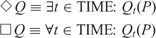
By these formulas we can introduce the temporal operators in a rather straightforward manner.

An observation (a predicate) Q is called stable, if the following proposition

holds for all processes P and all times t, t′.

1.5. System behaviors

A discrete system may show a set of behaviors represented by processes. In the literature a discrete system is often described by a state transition machine, for instance, or by a set of concurrent cooperating state machines, or by a Petri-Net. When executing such a state machine, actions are carried out that correspond to state transitions. Each instance of an action is an event. Thus, we associate for an interpreted process P (generated by the system) an action with each of its events.

Let E_p be the set of events forming a process P. The concept of a discrete interpreted process is defined by a mapping

where Action is the set of actions of the system. Each action defines a state change, a timing action or a communication action. This leads to a slightly more sophisticated notion of a system behavior represented by a set of processes where each event is timed and corresponds to an action.

1.6. Causality

Causality is a notion that is more sophisticated than that of time. Time is used to capture straightforward observations about systems. Referring to causality we speak about the rules (‘the logics’) for the occurrence of events and actions in the executions (processes) of systems.

Timing is an observation about a single process representing a run of a system. Causality speaks about the properties and rules that hold for all processes of a system and therefore deals with the logical properties of the system. Causality addresses the rules and thus the logics of systems.

But what is causality precisely and how is it related to the observations with respect to time?

Causality addresses the logical dependencies between the events and actions in the digital processes of a concurrent interactive system S. Causality actually deals both with liveness and safety in observations:

• • Liveness: Does observation A about the system S guarantee another observation B to follow later eventually: we say ‘in system S observation A leads_to observation B’.

• • Safety: Does observation B for the system S occur only if another observation A was observed before: we may write ‘in system S observation B ⇒ observation A’; however, this expression using implication does not properly express the relation between the two observations stating that B follows only after A, since the causal relationship is expressed rather implicitly this way.

For the concept of causality, the notion of the flow of actions and events in each process of the system is decisive, which reflects implicitly or explicitly a qualitative notion of time − more precisely an ordering of the events according to time.

Example: Airbag

Let us look at a simple example. An airbag in a car is activated only if the crash sensor indicates a crash, and whenever the crash sensor indicates a crash it is activated. Both observations are stable. Therefore, if we do not consider time flow, the two propositions: ‘crash sensor indicates crash’ (csic) and ‘airbag is activated’ (aia) are logical equivalent for completed processes.

The asymmetry of these two events with respect to the event flow of a system only gets modeled if we take the time flow into account. This can be done by studying sub-processes of the processes P representing the behaviors of cars. Then we require that

Here csic(P↓t) stands for ‘crash sensor indicates crash’ as one of the actions of an event in P↓t and aia stands for ‘airbag is activated’ as one of the actions of an event in P↓t.

These are examples of properties addressed by the notion of causality.

This example leads to a delicate question that addresses the difference between causality and logical implication. If we talk about the processes of a system and their sets of events without timing or causality information, we may easily write implications.

Example: Air Bag (continued)

For instance, in the case of an airbag we may write

This system property expresses that for each (complete) process of the airbag system this implication is valid. This seems fine. We are even tempted to read (*) as follows:

This is an assertion that can be appropriately formalized in temporal logic, but as a translation into the statement (*) above it is misleading, however, since it is an over-interpretation of implication. What we have written in (*) is simply logical implication. For the airbag we also assume the validity of the formula:

This is an implication like the one before. But now the ‘leads-to’ interpretation is no longer appropriate. A more accurate interpretation is: ‘If the air bag is activated then the crash sensor has indicated a crash before.’

In fact, one way to look at causality is to see it as a principle that can be observed in any form of information processing systems independently of their technical or physical representation. Causality addresses the logical dependencies between the events (and in turn the actions) of a system. Causality is a way to ‘understand’ a system. Certain events and actions may take place or not (such as input). Other events and actions can be caused by these events and actions (such as output). If a system has no rules of causality it is chaotic. Then all actions and events may occur at all times in a completely unrelated random manner.

Causality addresses both safety and liveness properties of systems. An event A may guarantee an event B to happen later. This relationship is what is called a liveness property. An event B may only happen if event A has happened before. This relationship is what is called a safety property.

There are basically two aspects of causality between two events (or actions) A and B. If A is causal for B, we may assume that

• • A enforces (leads_to) B: this means that whenever event A occurs event B eventually occurs (later),

• • B requires A: this means that event B does not occur if event A did not take place before.

Of course, there are many generalizations of the notion of causality beyond these two basic principles.

Example: Air Bag (continued)

For the airbag we obviously get the rules

as well as

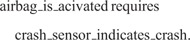
Here we have a typical example of a strong relation of causality.

Causality can be discussed not only in terms of events but also in terms of system properties. A property Q is called causal for a property Q′ if, for each system run, whenever we observe Q at some time t at some time later t′ > t we observe Q′. Moreover, whenever we observe Q at some time t′ there exists some time with t < t′ such that Q holds.

We say ‘observation A is causal for observation B in system S’ if for each process P ∈ S we have (for all times t ∈ TIME)

The first formula is capturing what is called the ‘leads-to’-property in temporal logic. It can be expressed by temporal logic as follows:

If both formulas shown above hold we speak of causality and write

From the definition of causality we easily prove the transitivity of the causality relation:

An observation is called stable for a process P, if

or in terms of temporal logic

In other words, if A holds at time t it remains valid from thereon. For stable observations causality is very close to logical equivalence. If A is causal for B and if A and B are stable then for each complete process P system causality boils down to implication:

Here, logically there is no asymmetry between A and B, which indicates that by simple implication the causal relationship between A and B is not modeled appropriately. Causality is reduced to logical equivalence when abstracting from timing. If we include timing the asymmetry between A and B becomes observable. There exist times t such that A(P↓t) holds but not B(P↓t). We get for all times t (recall that we assume that A and B are stable)

and

This shows that if A is causal for B we get B implies A which sounds counterintuitive since sometimes ‘implies’ may be confused with ‘leads to’.

A sophisticated question asks about the very nature of causality. If we assume in systems that there are mechanisms (‘algorithms’) that enforce that certain actions are executed by some control flow, this gives us a very concrete (‘operational’) idea of causality. On the other hand, we may develop some idea about causality only by observing systems and their generated actions and try to conclude causality relations from that.

Actually there are, along these lines, two ways to look at the causality of a system:

• • in an intentional approach (‘glass box view’) we study the internal structure and mechanisms of a system to recognize that certain events A are causal for certain events B due to the technical mechanisms (the ‘algorithmics’) that control the behavior and the flow of actions and events of the system.

• • in an extensional approach (‘black box view’) to causality we study only observations about a system in terms of its events and actions and their temporal relationships without any knowledge of the internal structure and mechanisms of the system. In the set of all observations we may recognize certain regularities that we then call causal dependencies.

In the first case we can speak about the causality within a single process or a single instance. In the second case we speak about the causality within the system considering all its processes. Both approaches lead to concepts and notions of causality. Extensional causality can be seen as an abstraction of intentional causality. By this abstraction some intentional causality may get hidden. We get a universal notion of extensional (‘observable’) causality for a system S modeled by its set of timed processes.

A simple example that illustrates this distinction between intentional and extensional is a non-deterministic process, where we have one run that first shows the action d that leads, due to its underlying mechanism, causally to the action b, and a behavior where the system can non-deterministically choose between the actions d or b. Then, intentionally in the first run, there is a causal relationship between d and b, while extensionally for the system this does not hold. Observationally, the intentional causality is hidden by the non-determinism of the system. An extensional causality is only valid if it is intentionally valid for all executions of the system.

If we can only observe runs of a system with the events and their timing we get processes that are sets of events with their timing. From the set of all observations we cannot, in general, derive the intentional causality. Intentional causality allows us to talk about the causality within a single execution represented by a process, while extensional causality considers a system as a whole with all its processes.

In spite of the example above, causality and non-determinism are independent notions. We do not even have to have a notion of non-determinism to introduce the concept of causality and vice versa.

2.1. What is a nondeterministic system

In the literature, there is a careful distinction between deterministic and non-deterministic systems. When looking at concrete system models, this distinction seems obvious, at a first sight. In fact, however, it is often not so clear how to give a definition of what it means that a system is ‘deterministic’ or ‘non-deterministic’. Often, abstractions turn deterministic system models into non-deterministic ones and vice versa.

The notion of non-determinism is inherently related to the notion of input to a system. If we consider systems without input from the outside, either the system has only one behavior (one run or one process) or it has to be considered as being non-deterministic. Input to a system comes from its environment and cannot be controlled by the system itself. Systems with a variety of choices for input are not considered non-deterministic if several processes depending on different input exist. Only if the system shows at least two different processes for the same input events do we call it non-deterministic.

We take here a very fundamental point of view. For us, a system is non-deterministic if its behavior includes choices that cannot be controlled by input from the outside but do influence its visible observable behavior.

2.2. Causality between input and output

For a system, there are events that are only internal and others that affect or are affected by the environment. Typical events of the second class are input and output. If we are aiming at an interface view of systems then we study the events at the border of a system, these being events that carry input or output across the system borders.

Of course, we may study models of systems where certain events carry both input and output; however, in the following we deal only with systems that show a clear separation between events providing input and those providing output in their externally visible events. Note that there exist system models (specific instances of so-called ‘process algebras’) like CSP or CCS (see Refs Reference Hoare2 and Reference Milner3) with the concept of synchronous communication where certain events are ‘shared’ between systems and their environments and thus may carry both input and output. Then there is no straightforward clear notion of causality between input and output.

We study a specific form of causality for systems in the following, namely the causality between their input and output events. We work under following hypothesis:

• • there is a canonical notion of extensional causality between input and output.

This idea of causality captures the essential relationship between input and output. For a system we assume that we have a clear notion of input, which means input events can be chosen arbitrarily by the environment (and must be accepted by the system). The input events form a sub-process called the input process. The system may or must react to such an input by an output. This manifests the fundamental principle of causality between input and output. Of course, in addition, there may be a causal relationship between the output events observable, which manifests some additional logics of the system.

In a deterministic system for each input process, exactly one output process is generated. Therefore, there is a fixed causality between the output events given some input process. In a non-deterministic system, several output processes may be possible for a given input.

Extensional causality is observed by studying all possible system processes or traces to find out whether an event is always present and guaranteed only after another event. This also applies for the causality between input and output. Such observations about the flow of events and their relationships are closely related to a model of time.

We work in the following with the simplifying assumption that we do not know anything about or at least do not take advantage of any causality in the input history. We are mainly interested in studying causality between input and output and the causality in the output history. This in turn also leads to a notion of causality in the output.

2.3. Information flow and causality

Whenever two subsystems of a system interact, and in this way mutually influence each other’s behavior within the context of the larger system, this requires a form of information exchange between the subsystems. In general, the information flows in both directions. This leads to a fundamental question:

• • Can we always model information exchange as a directed activity (information flow) with an explicit sender and one or several receivers (modeling mutual information exchange as two steps of directed information exchange)? The events of information exchange are then the output of one system and the input to the other.

The basic principle of causality in the information flow of components with input and output is as simple as the following axiom (here we assume that a system cannot predict its future input and thus there is no ‘anticipating logical gate’ – no logical gate that can predict its future input and thus produce a corresponding output before the input actually arrived; therefore, in real life systems, an output depending on such a future input can be produced only after that input had been received):

• • Information can only be evaluated, processed and forwarded as soon as/after it has been received.

This hypothesis leads to essential questions about the relationship between time, granularity, and causality. If the time granularity is fine enough there is always a delta, the ‘reaction time’, between the timing of the input and the output caused by it. If the time granularity is not fine enough, this does not hold, in general. In this case, input and output might occur in the same time interval and thus have the same time stamp.

2.4. Time granularity and causality

In this section we study changes and transformations of the time granularity of a system and its consequences. We are, in particular, interested in time abstractions that make the time scale coarser. Given a timed process P with the event set E and the timing function

we can change (‘transform’) the timing of the process P by a function

where we assume the following monotonicity property for all times t1, t2 ∈ TIME:

Given a time transformation function we get a new timing for process P by the function

specified by the formula (for all events e ∈ E)

As a result of a time transformation, the new timing may be coarser. Events e1 and e2 with the timing property time(e1) < time(e2) may become simultaneous events under time’. In other words, we may get time′(e1) = time′(e2). We speak of a time coarsening in this case.

We discuss in the remainder of this paper the notions of strong and of weak causality. Given strong causality, the time model strictly separates all events that are causal for other events from those for which they are causal. If we coarsen the timing of a process we may map a strongly causal process onto a process that is no longer strongly but only weakly causal.

We are interested to study in the following the effects of the time granularity and its coarsening onto the notion of causality. We study systems and their models under several time granularities.

Basically, for systems and their models we assume the following principles:

• • For the time granularity we find:

  • • If the time scale of the input events is chosen fine enough then there is no non-determinism/underleft in the system model that is due to missing information about the timing of the input.

  • • If the time scale is finer than the minimal delay of reactions to events, then causal events are separated by time and the behavior is strongly causal.

  • • Every system behavior is weakly causal in appropriately constructed system models. Strong causality, however, may be abstracted away due to time models that are too coarse and hence do not separate some events that are in the causality relation.

  • • Every system behavior is ‘physically’ strongly causal. This means that even for a given weakly causal model of a real-world system there exists a strongly causal behavior model such that the given weakly causal system behavior model is a time coarsening of this strongly causal model.

If we choose the time granularity not fine enough then we get a system behavior that is only weakly causal, although implicitly strongly causal since it is an abstraction of a strongly causal system.

3.1. Streams

A stream is a finite or infinite sequence of elements. In interactive systems streams are built over sets of messages, signals, or actions. Streams are used in that way to represent communication histories for sequential communication devices such as channels or for sequential histories of activities.

Let M be a given set of messages. A stream over the set M is a finite or an infinite sequence of elements from M.

We use the following notation:

M*

denotes the set of finite sequences over M including the empty sequence 〈〉,

M^∞

denotes the set of infinite sequences over M (that are represented by the total mappings IN\{0} → M).

A stream is a member of the set M^ω that is defined by the equation

We introduce the prefix ordering ⊑ on streams, which is a partial order specified for streams x, y ∈ M^ω by the formula

Here, x ^∧z denotes the well-known concatenation of sequences; by concatenation the stream z is appended to the stream x. To extend the concatenation to infinite streams we define: if x is infinite then x ^∧z = x.

Throughout this paper, we do not work with this simple concept of a stream as introduced above. Since we want to deal with the timing of systems we find it more appropriate to use so-called timed streams. An infinite timed stream represents an infinite history of communications over a channel or an infinite history of activities that are carried out sequentially in a discrete time frame. The discrete time frame represents time as an infinite chain of time intervals of equal finite duration. In each time interval a finite number of messages can be communicated or a finite number of actions can be executed. Since we do not assume anything about the speed of communication the sequence of messages communicated within a time interval can be arbitrarily long but it is always finite.

Therefore, we represent a communication history over a sequential communication medium in a system model executed in a discrete time frame by an infinite sequence (a ‘stream’) of finite sequences of messages or actions. By

we denote the set of timed streams. Note that the elements of (M*)^∞ are infinite streams of finite sequences.

The idea of a timed stream reflects directly the concept of an observation in a discrete time scale. For every time t ∈ IN and every stream s ∈ (M*)^∞ the prefix of s of length t (which is a sequence of length t of finite sequences from M*) reflects the observation until time t.

For a function f we often write f.z for function applications instead of f(z) to avoid unnecessary brackets.

Throughout this paper we work with a couple of simple basic operators and notations for streams that are summarized below:

〈〉

empty sequence or empty stream,

〈m〉

one-element sequence containing m as its only element,

x.t

tth element of the stream x, which is a sequence in the case of a timed stream

x

length of the stream x,

x ^∧z

concatenation of the sequence x to the sequence or stream z,

x↓t

prefix of length t of the stream x (which is a sequence with t elements; in the case of a timed stream, a sequence with t sequences as elements), provided x has at least t elements (otherwise x↓t = x),

S©x

stream obtained from x by deleting all its messages that are not elements of the set S.

For a timed stream we denote by

the finite or infinite stream that is the result of concatenating all sequences in the timed stream x. Note that is finite if x carries only a finite number of non-empty sequences.

A timed stream x ∈ (M*)^∞ carries the information at which times which messages are transmitted. As long as the timing is not relevant for a system it does not matter if a message is transmitted somewhat later (scheduling messages earlier may make a difference with respect to causality – see later). To take care of this we introduce the concept of a ‘delay closure’.

For a timed stream x ∈ (M*)^∞ we define the delay closure of x by the set x↑ of timed streams that carry the same stream of messages but perhaps with some additional time delays as follows:

Obviously, we have x ∈ x↑ and for each x′ ∈ x↑ we have

as well as

The set s↑ is called the delay closure for the stream s. The delay closure is easily extended from streams to sets of streams by pointwise application (let S ⊆ (M*)^∞)

Throughout this paper, we use streams exclusively to model the communication histories of sequential communication media that we call channels. In general, in a system, many communication streams occur. Therefore, we work with channels to name the individual communication streams. Accordingly, in Focus, a channel is simply an identifier in a system that identifies a communication line and in every execution of the system it evaluates a stream of messages communicated over that line.

3.2. Components: syntactic and semantic interfaces

In this section we introduce a mathematical notion of components and their interfaces. Components interact with their environment via channels. A channel is a communication link and is uniquely identified by a channel identifier.

3.2.1. I/O-behaviors

Types (or sorts) are useful concepts to describe interfaces. We work with a simple notion of types where each type represents a set of data elements. These data elements are used as messages or as values of state attributes.

Let a set S of types of messages be given. By M where

we denote the set (the ‘universe’) of all data messages.

In Focus a typed channel is an identifier for a sequential directed communication link for transmitting messages of that type. By C we denote a typed channel set. We assume that a type assignment for the channels in the set C is given by the mapping:

Given a set C of typed channels, a channel valuation is an element of the set defined as follows:

A channel valuation associates a stream of elements of type type(c) with each channel c ∈ C. In this way the channel valuation x defines a communication history for each of the channels in the set C. The operators on streams induce operators on channel valuations and furthermore on sets of streams as well as sets of channel valuations by pointwise application. In this way all our operators introduced on streams generalize to channel valuations.

Given a set of typed input channels I and a set of typed output channels O we introduce the notion of a syntactic interface of a component:

(I, O)

syntactic interface,

I

set of typed input channels and,

O

set of typed output channels.

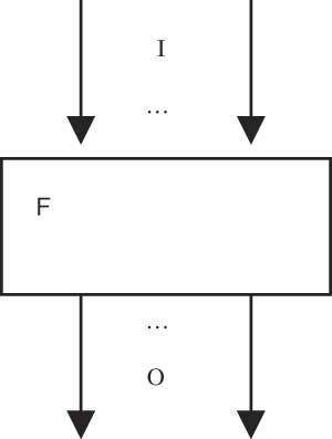
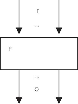
A graphical representation of a component and its interface as a data flow node is shown in Figure 1. We do not require that the channel sets I and O are disjoint. If a channel c occurs both in I and O it denotes two different channels: one channel in the set of input channels and one channel in the set of input channels.

Figure 1

Graphical Representation of a Component F with the Set of Input Channels I and the Set of Output Channels O.

For a component-oriented approach to system development in addition to the syntactic interface, a concept for describing the behavior of a component is needed. We work with a simple and straightforward notion of a behavior. Relations between input histories and output histories represent behaviors of systems. Input histories are represented by valuations of the input channels and output histories are represented by the valuations of the output channels.

In Focus, we represent the black box or interface behavior of systems by set-valued functions (we also speak of the semantic or behavioral interface of the component):

As is well known, such a set-valued function is isomorphic to a relation that is a subset of . We prefer set-valued functions in the case of system behaviors to emphasize the different roles of input and output. We call the function F an I/O-behavior. Given an input history , F.x denotes the set of all output histories. A system with behavior F may exhibit anyone of these in reaction to the input x.

An I/O-behavior F is called deterministic, if F.x is a one-element set for each . A deterministic I/O-behavior represents a function .

It is well known that a naive modeling of the behavior of systems by relations on streams leads into the so-called merge anomaly (also called Brock-Ackermann anomaly, see Ref. Reference Brock and Ackermann6). In Focus, this anomaly is avoided by the notion of strong causality (see later).

3.3. Specification of I/O-behaviors

An I/O-behavior represents a model of the behavior of a system. Using logical means, an I/O-behavior F can be described by a logical formula, called a specifying assertion relating the streams on the input channels to the streams on the output channels. In such a formula, channel identifiers occur syntactically as identifiers (variables) for streams of the respective type. The specifying formulas are interpreted in the standard way of typed higher-order predicate logic (see Ref. Reference Andrews7).

An abstract specification of a system provides the following information:

• • its syntactic interface, describing the input and output channels by which the system interacts with its environment,

• • its behavior by a specifying formula Φ relating input and output channel valuations.

This leads to a specification technique for systems (see Ref. Reference Broy and Stølen4 for lots of examples). In Focus we specify a system by a scheme of the following form:

〈name〉

in 〈input channels〉

out 〈output channels〉

〈specifying formula〉

The shape of the scheme is inspired by well-known specification approaches like Z (see Ref. Reference Spivey8).

Example. Transmission, merge and fork

As simple but quite fundamental examples of systems we specify a merge component MRG, a transmission component TMC, and a fork component FRK. In the examples, let T1, T2, and T3 be types (recall that in our case types are simply sets) where T1 and T2 are assumed to be disjoint and T3 is the union of the sets of elements of type T1 and T2. The specification of the merge component MRG (actually the specification relies on the fact that T1 and T2 are disjoint, which should be made explicit in the specification in a more sophisticated specification approach) reads as follows:

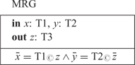
In this specification we do not specify the quantitative timing (since the output does not refer to or depend on the timing of the input of the output streams) and therefore we refer only to the time abstractions of the involved streams. The causality of the time and message flow is considered in detail in the following subsection.

We specify the proposition x∼y for timed streams x and y of arbitrary type T; x∼y is true if the messages in x are a permutation of the messages in y. Formally, we define this operator by the following logical equivalence relation:

Based on this definition we specify the component TMC below.

Often it is helpful to use some channel identifiers both for input channels and for output channels. These are then actually two different channels, which, of course, may have different types. To distinguish these channels in the specifying formulas, we use a well-known notational convention. In a specification, it is sometime convenient to use the same channel name for an input as well as for an output channel. Since these are different channels with identical names we have to distinguish them in the body of a specification. Hence, in the body of a specification, we write, for a channel c − which occurs both as an input and as an output channel − simply c to denote the stream on the input channel c, and c′ to denote the stream on the output channel c. Thus, in the following specification, z is the outside name of the output channel z, and z′ is its local name used in the specifying formula.

TMC

inz: T3

outz: T3

z∼z′

This simple specification says that for component TMC every input message occurs eventually also as an output message, and vice versa. Nothing is specified about the timing of the messages. In particular, messages may be arbitrarily delayed and overtake each other. Output messages may even be produced earlier than they are received. This paradox is excluded by causality in the following section.

The following component, FRK, is just the ‘inversion’ of the component MRG.

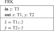
Note that the merge component MRG as well as the TMC component and the fork component FRK as they are specified here are ‘fair’. Every input is eventually processed and reproduced as output.

Based on the specifying formula given in a specification of an I/O-behavior, F, we may prove properties about the function F in classical (higher order) predicate logic.

3.4. Causality and timing in I/O-behaviors

For input/output information processing devices, the notion of causality is crucial. Certain output depends causally on certain input. Causality indicates dependencies between the input and output actions of information exchange of a system. So far I/O-behaviors are nothing but relations represented by set-valued functions. In the following we introduce and discuss the notion of causality for I/O-behaviors.

I/O-behaviors generate their output and consume their input in a global time frame. This time frame is useful to characterize causality between input and output. Output that depends causally on certain input cannot be generated before this input has actually been received.

Let an I/O-behavior

be given. In the following we define a couple of fundamental notions to characterize specific properties of F that relate to causality and the timing of the input and output messages.

Definition: Weak causality for component behavior

An I/O-behavior F is called weakly causal (properly timed), if for all times t∈IN the following formula is valid

F is properly timed if the output in the tth time interval does not depend on input that is received after time t. This ensures that there is a proper time flow for the component modeled by the behavior function F. This is a property that manifests the essential asymmetry between input and output.

If F is not weakly causal then there exists a time t and input histories x and x′ such that x↓t = x′↓t but (F.x)↓t ≠ (F.x′)↓t. A difference between the input histories x and x′ occurs only after time t, but at time t the reactions of F in terms of its output messages until time t are already different.

Nevertheless, proper timing in terms of weak causality does not exclude instantaneous reaction (see Ref. Reference Berry and Gonthier9): the output at time t may depend on the input at time t. This may, however, lead into problems with causality if we consider, in addition, delay free feedback loops (such problems also occur in EsterelReference Berry and Gonthier⁹). To avoid these problems we better strengthen the concept of proper time flow to the notion of strong causality.

Definition: Strong causality for component behavior

An I/O-behavior F is called strongly causal (or time guarded), if for all times t∈IN (and all input histories x and z) we have

If F is time guarded then the output in the tth time interval does not depend on input that is received after the (t−1)th time interval. Then F is certainly properly timed and, in addition, reacts to input received in the (t−1)th time interval, and not before the tth time interval. In this way, causality between input and output is guaranteed and explicitly visible according to the sufficiently fine time granularity.

Definition: Delay by n time units

We write delay(F, n), if F is a behavior with a delay by (at least) n time units. More precisely we define:

In other words, F is (weakly) causal if delay(F, 0) holds and strongly causal if delay(F, 1) holds.

Obviously we have for all n, m∈IN (the proof is straightforward):

If delay (F, ∞) holds then the output does not depend on the input at all.

For a weakly causal component there is always a maximal number n∈IN ∪ {∞} such that delay(F, n) holds. This number is called the guaranteed delay.

Our concept of delay is easily extended to individual output channels. Of course, there may be different delays and different guaranteed delays valid for the different output channels of an I/O-behavior. We will return to this.

A function is called weakly or strongly causal respectively if the deterministic I/O-behavior specified by F.x={f.x} for all has the required properties.

By [F] we denote the set of time guarded total functions , with f.x ∈ F.x for all input histories .

A non-deterministic specification F defines the set [F] of total deterministic behaviors. A specification is only meaningful (‘consistent’) if the set [F] is not empty. This idea leads to the following definition.

Definition: Realizability

An I/O-behavior F is called realizable, if [F] ≠ Ø; this means that there exists a time guarded total function such that

Given an input an output is called realizable for F with input x, if there is a function f∈[F] such that y = f.x.

A time guarded function provides a deterministic strategy to calculate for every input history x a particular output history y which is correct for F, i.e. such that y ∈ F.x holds. Every input x↓t until time point t fixes the output until time point t+1 and in particular the output at time t + 1. Actually the function f essentially defines a deterministic automaton with input and output.

If an I/O-behavior F is not realizable there does not exist a state machine that implements it, not even a state machine that implements a refinement of F (for a proof, see Ref. 11).

There are sophisticated examples of behaviors that are strongly causal, but not realizable. Consider for instance the following example of a behavior that is not realizable (here the proof of this fact is left to the reader, a proof can be found in Ref. Reference Broy and Stølen4):

Note that this behavior F is strongly causal but not realizable.

Definition: Full realizability

An I/O-behavior F is called fully realizable, if it is realizable, and if for all input histories :

holds.

Full realizability guarantees that for all output histories there is a strategy (a deterministic state machine implementation) that computes this output history. For fully realizable behavior there is a close relationship between F and the set [[F]]. Both define the behavior of a system. In fact, non-deterministic state machines with input and output are not more powerful or more expressive than sets of deterministic state machines with input and output. An extensive definition of realizability and its relation to computability can be found in Ref. 11.

3.5. Property refinement of interfaces

Property refinement allows us to replace an interface behavior by one having additional properties. In this way, interface behaviors are replaced by a more restricted ones. An interface

is refined by a behavior

If

We then write

Obviously, property refinement is a partial order and therefore reflexive, asymmetric, and transitive. Note that the paradoxical system, with empty sets of output histories for each of its input histories, is logically a refinement for every system with the same syntactic interface.

A property refinement is a basic refinement step, adding requirements as is done step by step in requirements engineering.

3.6. Computations

Our model describes behavior in terms of the relationship between input and output histories. In this section, we show how to associate computations with behaviors. The key idea is that we calculate the output in each time interval step by step from the input given in the previous time interval according to the progress of time.

We show how to calculate stepwise inductively an output history for a given strongly causal realizable behavior F and an input history that is only provided stepwise. We construct the output histories defining y↓t iteratively from input x↓t for t = 0, 1, 2, … The key idea is that we can select the output y.t+1 given x↓t without considering x.t + 1.

We define a computation for a realizable behavior F for a given input history inductively as follows: we choose a deterministic behavior f ∈ [F].

We start with t = 0; by definition x↓0 and y↓0 are both empty histories. Given x↓t and y↓t ∈ (F.x)↓t we construct from x↓t and y↓t the sequence y.t + 1 as follows.

We construct a chain of partial output histories y_t ∈ (F.x)↓t such that

The construction works as follows: we start the iteration with the empty history:

Given y_t we construct y_{t + 1} by the following rules:

1. (1) choose some y′ ∈ {f.x′: x′↓t = x↓t}

2. (2) define y_{t + 1} = y_t ^∧〈y′.t + 1〉

Note that by strong causality y_t = y′↓t and thus y_{t +1} = y′↓t + 1. This shows that our construction essentially relies on the strong causality of f.

If the behavior is not strongly causal, then our construction does not work, in general. Given some input x↓t we may select some output

such that

The partial output y↓t therefore cannot be necessarily completed into a complete infinite output history (for details, see Ref. 11).

The same applies if the output y is not realizable. Then a function f ∈ [F] does not exist with y = f.x. If we would choose in step (1) the formula y′ ∈ {F.x′: x′↓t = x↓t} then it is not guaranteed that y ∈ F.t holds with this construction. For a behavior function there may exist a history such that for some input history we have y↓t ∈ (F.x)↓t for all t but y ∉ F.x (for details see Ref. 11).

3.7. Fixpoints

To compose two or more components into a system architecture these components are connected by their channels. Some of these connecting channels typically form feedback loops, in general. Feedback corresponds to recursive definitions of the streams in the channel valuations. Recursion on streams is treated, as usual, in terms of ‘fixpoints’.

As is well-known, deterministic strongly causal functions always have fixpoints. Strongly causal function are guarded and thus the fixpoints can be ‘inductively’ defined. The existence proof basically is given by an inductive construction of the fixpoint along the lines of the definition of the concept of a computation as shown above. Thus, realizable strongly causal behaviors always have fixpoints that reflect feasible computations of the system.

Recall, that every strongly causal function

has a unique fixpoint x = f(x). The proof is quite straightforward by an inductive construction of the fixpoint as in the previous section on computations. Therefore, every realizable function

has a fixpoint x ∈ F(x). (Note that, for a function F that maps histories onto sets of histories, x is called a fixpoint if x ∈ F(x).) Moreover, for a fully realizable behavior, every fixpoint x ∈ F(x) is a fixpoint of a function f ∈ [F].

Using weakly causal functions we run into difficulties, here, however, to separate fixpoints x ∈ F(x) that correspond to actual computations from those that do not. In the case of strongly causal, realizable functions, every fixpoint corresponds to a proper computation. For a weakly causal function

we do not even have a guarantee that fixpoints actually exist.

Example: Fixpoints for weakly and strongly causal functions

Consider as an example the following specification:

Succ

ina: IN

outb: IN

∀ t: b.t=ifa.t=〈〉 then 〈1〉 else succ*(a.t) fi

where ∀ n ∈ IN, s ∈ IN*:

succ*(〈〉)=〈〉

∧ succ*(〈n〉^∧s) = 〈n + 1〉^∧succ*(s)

Succ is obviously weakly causal, but not strongly causal since the output at time t depends exclusively on the input at time t. However, Succ does not have a fixpoint x ∈ Succ.x; this is proved by contradiction as follows; there does not exist a history x and y with

since this would immediately result in a contradiction because then for all times t ∈ IN we would get (with a.t = b.t):

which is an equation impossible to fulfill since if b.t = 〈〉 then b.t = 〈1〉 would follow as well as b.t ≠ 〈〉 and b.t = succ*(b.t) cannot hold. If we slightly change the definition by writing b.t + 1=… instead of b.t=… then the specified behavior is obviously strongly causal and fixpoints do exist. One fixpoint (in fact the only one) is then given by the timed stream on channel b:

b.0 = 〈〉

b.1 = 〈1〉

b.2 = 〈2〉 …

This example demonstrates the complications when working with only weakly causal in contrast to strongly causal functions and behaviors. Such problems are also encountered in approaches called ‘perfect synchrony’ as found in Esterel,Reference Berry and Gonthier⁹ leading to the well-known problem of certain Esterel programs called causal loops that are without proper computations.

4.1. Composing components

Given I/O-behaviors

where the sets of output channels are disjoint

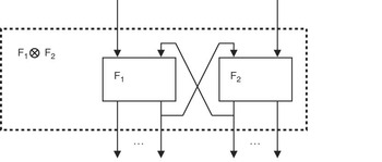
we define the parallel composition with feedback as it is illustrated in Figure 2 by the I/O-behavior

with a syntactic interface as specified by the equations:

The resulting function is specified by the following equation (here we assume where the set of all channels C is given by C = I₁ ∪ I₂ ∪ O₁ ∪ O₂):

Here for a channel set C′ ⊆ C we denote for by z|C′ the restriction of y to the channels in C′. The equation defining composition includes a fixpoint construction for all channels in

For these channels for given input history we get, by the notation above, some which is a fixpoint of the function

where, for ,

is defined as follows:

As long as F₁ and F₂ have disjoint sets of input and output channels the composition is simple. Given and we get the equation

Now assume

Note F₂ is then the component without input and output. We write then μ.F₁ for F₁ ⊗ F₂. We get I = Ø (μ.F₁ has no input channels) and

This somewhat special construction shows once more that composition with feedback loops corresponds to a kind of fixpoint equation. We call y ∈ F₁.y a fixpoint of F₁. Note in the case of a deterministic function we get y = f₁.y.

Figure 2

Parallel composition with feedback.

The operator ⊗ is a rather general composition operator that can be easily extended from two components to a family of components.

A more specific operation is sequential composition also called pipelining. It is a special case of the composition operator where O₁ = I₂ and the sets I₁ and O₂ are disjoint. In this case we define

where the composition is illustrated by Figure 3.

Figure 3

Pipelining.

Pipelining is the special case of composition without feedback. It can easily be generalized to the case where the channel sets I₁ and O₂ are not disjoint. The definition reads as follows

This composition is also called relational composition if F₁ and F₂ are represented as relations or functional composition if F₁ and F₂ are deterministic and thus functions.

4.2. Granularity refinement: changing levels of abstraction

In this section we show how to change the levels of abstractions by refinements of the interfaces, state machines and processes. Changing the granularity of interaction and thus the level of abstraction is a classical technique in software system development.

Interaction refinement is the refinement notion for modeling development steps between levels of abstraction. Interaction refinement allows us to change for a component

• • the number and names of its input and output channels,

• • the types of the messages on its channels determining the granularity of the communication.

An interaction refinement is described by a pair of functions

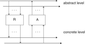
that relate the interaction on an abstract level with corresponding interaction on the more concrete level. This pair specifies a development step that is leading from one level of abstraction to the other, as illustrated by Figure 4. Given an abstract history each y ∈ R(x) denotes a concrete history representing x. Calculating a representation for a given abstract history and then its abstraction yields the old abstract history again. Using sequential composition, this is expressed by the requirement:

Let Id denote the identity relation, and ‘°’ the sequential composition is defined as follows:

A is called the abstraction and R is called the representation. R and A are called a refinement pair. For untimed systems we weaken this requirement by requiring R°A to be a property refinement of the untimed identity, formally expressed by the following equation:

This defines an identity under time abstraction.

Figure 4

Communication history refinement.

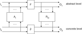
Interaction refinement allows us to refine systems, given appropriate refinement pairs for their input and output channels. The idea of an interaction refinement is visualized in Figure 5 for the so-called U⁻¹-simulation. Note that here the components (boxes) A_I and A_O are no longer definitional in the sense of specifications, but rather methodological, since they relate two levels of abstraction.

Figure 5

Interaction refinement (U ⁻¹-simulation).

Given refinement pairs

for the input and output channels we are able to relate abstract to concrete channels for the input and for the output. We call the interface

an interaction refinement of the I/O-behavior

if the following proposition holds: ≈>

This formula essentially expresses that is a property refinement of the system A_I ° F ° R_O. Thus, for every ‘concrete’ input history every concrete output can also be obtained by translating onto an abstract input history such that we can choose an abstract output history y ∈ F(x) such that .

5.1. Changing the time scale

Let n ∈ IN with n > 0 and C be a set of typed channels; to make, for a channel history (or a stream)

its time scale coarser by the factor n we introduce the coarsening function

defined by (for all t ∈ IN):

COA(n).x yields a history from history x where for each stream associated with a channel the sequences for n successive time intervals are concatenated (‘abstracted’) into one. In that way we forget about some of the time distributions of x. The time scale is made coarser that way.

Time coarsening, obviously, is an instance of abstraction. We forget some information about the timing of a history. The mapping is not injective. Distinct histories may be mapped onto the same history by time scale coarsening.

It is not difficult to allow even a coarsening factor n = ∞ in time coarsening. Then, the infinite number of time intervals in a timed stream is mapped into one. The infinite stream of sequences is concatenated into a non-timed stream. Timed streams are abstracted into non-timed streams in that way if we define:

On histories, coarsening is a function that is not injective and thus there does not exist an inverse.

We generalize the coarsening of the time scale from channel histories to behaviors. We coarsen both the input and the output histories. To make a behavior

coarser by the factor n, we define the coarsening operator that maps F onto a function

which is defined as follows

Coarsening maps I/O-behaviors onto I/O-behaviors. On one hand, coarsening may introduce further non-determinism and underspecification into behaviors due to the coarser time scale of the input histories. Certain different input histories are mapped by the time coarsening onto the same coarser input histories. Then their sets of output histories are defined by the union of all their coarsened output histories. In this way non-determinism may grow.

On the other hand, some non-determinism and underspecification may be removed in behaviors by coarsening since some different output histories may be mapped by the time coarsening onto the same coarser output history.

A special case is the coarsening COA(F, ∞), which abstracts completely away all time information. If the output of F depends on the timing of the input, then the coarsening COA(F, ∞) introduces a lot of non-determinism, in general. However, if the output produced by F does not depend on the timing of the input messages at all but only on their values and the order in which they arrive, COA(F, ∞) will rather be more deterministic.

If F is weakly causal, the behavior COA(F, n) is obviously also weakly causal. However, strong causality is not maintained by coarsening the time scale. We will return to more explicit laws of causality and coarsening later. Reactions to input at later time intervals may be mapped onto one time interval.

We can also map a history as well as a behavior onto a finer time granularity. Let n ∈ IN; to make for a history (or a stream)

its time scale finer by the factor n we use the function

defined by the equation:

FINE(n).x yields the set of histories where for each time interval the sequences of messages in this interval are arbitrarily subdivided into n sequences that are associated with n successive time intervals. Thus, the sequence on each time interval for each channel is non-deterministically divided into n sequences. The time scale is made finer that way.

Making the time scale finer is a form of concretization in contrast to abstraction. Each history is mapped onto a number of histories by making its time scale finer. Each of these histories represents one version of the history with a finer time granularity.

Another way to define the function FINE is demonstrated by the following formula

This equation shows more explicitly the relationship between making the time scale coarser and making the time scale finer. They are ‘inverse’ operations (for detailed discussion see the following section). Changing the time scale represents an abstraction if we make the time scale coarser, and a concretization if we make it finer.

The idea of making a time scale finer can be applied also to behaviors. We specify

Due to the underspecification that is involved in the way we make the time scale finer, there is no guarantee that we get a higher number of delays in the behaviors when moving to a finer time scale.

Nevertheless, we can introduce an ‘artificial’ operator DFINE that makes the time scale finer in a way that guarantees a larger delay. This operator is easily defined in a brute force way by defining DFINE as follows for t ∈ IN\{0}

Then every input is delayed by the factor n.

Such an operator is artificial, however, since it resolves some of the non-determinism introduced by the operator FINE in a brute force way by making the time grain finer in a way that guarantees the largest delay.

Going from a finer to a coarser time scale we generally lose some information about the timing that cannot be recovered properly when making the time scale finer again.

5.2. Rules for time scale refinement

Changing the time scale is an operation on histories and behaviors. In this section we study laws and rules for changing the time scale.

Our first rules for changing the time scale show that the functions COA(n) and FINE(n) form refinement pairs in the sense ofReference Broy and Stølen⁴

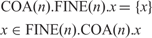
In other words, coarsening is the inverse of making the time scale finer. The proof of the equation is quite straightforward by the definition of COA and FINE.

We observe, in particular, the following equations (here F₁°F₂ denotes the pipeline composition of and 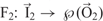where O₁ = I₂ and (F₁ ° F₂ ).x={y: ∃z: z ∈ F₁.x ∧ y ∈ F₂.z})

The proof is again quite straightforward. The equations show that time refinement in fact is a special case of interaction granularity refinement (see Ref. 12).

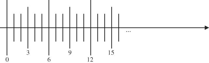
Both time granularity abstractions and refinements by factors n*m can be seen as two consecutive refinements by the factor n followed by a refinement with factor m or vice versa.

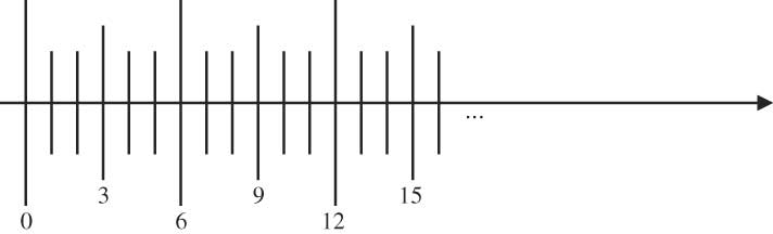
Figure 6 shows such an iterative refinement of the time scale.

Figure 6

Refinement of the time scale by 6: shown as a refinement by the factor 3 followed by a refinement by the factor 2.

Figure 7

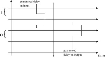
Relationship between input with guaranteed delay and output with guaranteed delay at time t.

We get the following obvious rules:

We are, in particular, interested to analyze how time refinement relates to causality. This relationship is illustrated by the following equation (let m, n ∈ IN with m ⩾ 1):

The proof of this rule is quite straightforward and uses the fact that

holds.

This rule is, in particular, interesting for our discussion of time, time abstraction, and causality. As long as we coarsen a behavior F for which delay(F, n) holds at most by factor n, causality is still guaranteed for the resulting component.

In fact, there exists a kind of monotonicity of coarsening with respect to delay properties:

Again the proof is straightforward and left to the reader. If we coarsen the time scale we may, in general, lose strong causality. In other words, the property of strong causality depends on a fine enough granularity of the time scale.

The following equation does not, in general, hold for the operator FINE. It holds only for the version DFINE of FINE that increases the delay.

To keep this formula valid we cannot replace the operator DFINE by FINE.

5.3. Fractions of time changes

For a given behavior F we can change its timing by fractions m/n for m, n ∈ IN using the time change operator TCH.

Note that all the rules introduced so far for COA and FINE obviously carry over to this case, since we expressed TCH in terms of COA and FINE.

5.4. Choosing the appropriate time scale

We have discussed how closely the time scale is related to the property of causality. It depends very much on the time scale whether a behavior is strongly causal as well as on the delay properties of the components. In a large system with many components, different time scales may be appropriate for different subsystems. In the remainder of this section we therefore study an idea of flexible timing.

Complex hierarchical distributed systems require a flexible time model such that its time granularity can be adapted individually to the needs of its various subsystems.

This leads to the following idea: we establish and model different time scales for the subsystems of a composed system. Then we can choose the time scales in a flexible way, according to the following observations:

• • for each system composed of strongly causal components its time delay is greater than the length of the shortest path of channels through the system of components;

• • therefore we can coarsen the interface abstraction of the system by the factor k without losing strong causality provided the shortest path is ⩾ k.

This leads to hierarchical system models that support local islands (‘subsystems’) of finer granularity of time. A system may be composed of many subsystems with their own finer time scales. To discuss this idea in detail we have first to introduce a notion of composition.

5.5. Causal fixpoints and causal loops

Given a strongly causal function

each fixpoint y ∈ F.y is called causally faithful or, for short, causal. In a causal fixpoint, each sequence of values in a time interval t is triggered by the values that occurred in the history before t.

Now we consider a coarsening of the time for the function F

We get for each fixpoint

that COA(n).y is a fixpoint of COA(F, n), too. But there may be fixpoints COA(F, n) that do not correspond to fixpoints of F.

A fixpoint y′ ∈ (COA(F, n)).y′ is called causal w.r.t. F if there is a fixpoint y ∈ F.y such that y′=COA(n).y. Otherwise y′ is called a causal loop.

We will show that considering COA(F, n) alone without knowing F we cannot distinguish, in general, causal fixpoints from causal loops. In other words, if we choose the time scale too coarse such that the resulting function is not strongly causal we may lose the faithful notion of causality and compositionality and cannot distinguish causal from not causal fixpoints.

Let us consider a simple function

with the specification (for all channels c ∈ C)

IDS is the identity on the data streams shifted by one time interval.

Now we consider the history

we get

This shows that x is not a fixpoint of IDS. Now we consider COA(2).IDS. We get:

This proves the fixpoint property

So 〈〈1〉〉^∞ is a fixpoint of COA(2).IDS. However, this fixpoint is not causal, since 〈〈〉〉^∞ is the only fixpoint of IDS as well as COA(IDS, 2).

This shows that coarsening a behavior F leads to functions F′ with additional fixpoints that are not causal in the case that F′ is, in contrast to F, not strongly but only weakly causal. Moreover, we cannot distinguish, in general, for these functions between causal and non-causal fixpoints.

5.6. Delay calculus for system architectures

By composition of a family of components we can form a network (representing an architecture) of components with delays. This network is a directed graph with channels as arcs and components as nodes.

With each path in the graph leading from an input channel to an output channel c, we can associate a delay, which is the sum of all delays on that path (each component on the path adds to the delays). For an output channel c the (guaranteed) delay in the system for c is the minimum over the sum of delays on each of the paths from some input channel to the output channel c.

In a behavior function we can define the guaranteed delay between an input channel and an output channel. Consider

and an output channel c′ ∈ O and an input channel c ∈ I. We define the guaranteed delay for the output channel c in F by the following formula (Figure 7 illustrates the relationship between delayed input and guaranteed delay of the output):

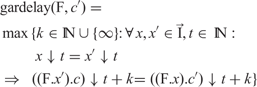
In a composed system we define the delay length of a path from an input channel c′ to an output channel c as follows:

A path is a sequence of channels p = 〈c ₀c ₁ … c _k〉 such that for each index i < k there exists a component F_i in the system such that c _i is an input channel of F_i and c _{i +1} is an output channel of that component. c ₀ is called the source of p and c _k is called the target of p. By Path(c, c′) we denote the set of all paths with source c and target c′.

The delay length of the path is given by the formula

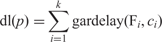
For each output channel c′ for the system F represented by the considered network we obtain:

Given lower bounds for the delays between the components we can calculate lower bounds for the delays for output channels in composed systems.

5.7. Composition and delay

Using our composition operators we can construct system architectures represented by data flow nets. In this section, we study how to calculate the delay of composed systems from the delay profile of their components. For each component of the considered system, we can define a (maximal) guaranteed delay for each output channel. Given a component

we introduce mappings

that associate a delay with every input and output channel. To calculate the guaranteed delay of a network of components, we have to be able to determine the delay of F if for each of its input channels a delay is given.

We are interested in the delay of a component that is inside a large architecture given by a data flow graph (with feedback loops). If we give input to the data flow graph up to time t ∈ IN then we assume that for each channel c ∈ I the stream (x.c)↓(t + d.c) determined by that input to the network up to time t.

From this delay of the input we guarantee a delay for the output channels at time t, if d.b is the guaranteed delay on input channel b∈I; thus the input (x.b)↓(t + d.b) is fixed at time t. We write

for the logical proposition that holds, if for all times t ∈ IN we have (here we assume that for a stream s the partial stream s↓j is empty if j ⩽ 0)

This formula expresses that the input on channel b affects the output on channel c at most after e.c time steps, provided fresh input arrives on the input channels only after the times as described by d. We call then the functions

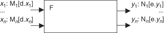
a delay profile. A delay profile can be graphically represented by an annotated data flow node as show in Figure 8.

Figure 8

Delay profile in a graphical representation.

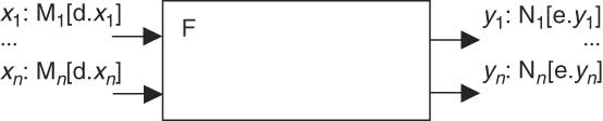
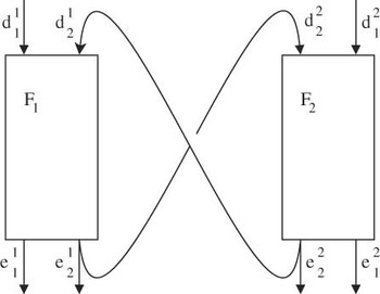
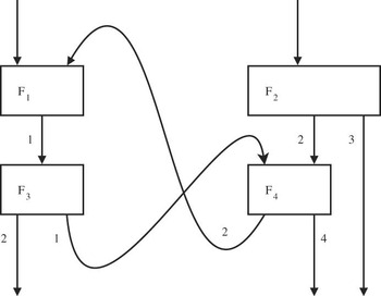
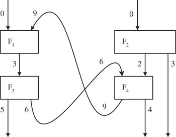
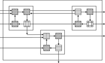
Let all the definitions be as in the section on composition. For a composition we get graphical representations of the delay profiles of the components as shown in Figure 9.

Figure 9

Delay profile for the components in a composition (suppressing channel identifiers).

Given

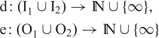
we only have to assume for d^k = d|I_k and e^k = e|O_k for k = 1, 2:

as well as

and for the feedback (by we denote the vector of delays for the channels in (I₁ ∩ O₂), by 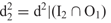we denote the vector of delays for the channels in (I₁ ∩ O₂), by 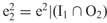we denote the vector of delays for the channels in (I₁ ∩ O₂), by we denote the vector of delays for the channels in (I₁ ∩ O₂))

to guarantee

Note that the guaranteed delay of a feedback channel c ∈ (I₁ ∩ O₂) ∪ (I₂ ∩ O₁) must be greater at the output than the assumed at the input to guarantee a faithful fixpoint and strong causality. This way of asserting delays of composition can be captured in a simple proof rule.

Figure 10

Network of components with given delay for each channel.

Figure 11

Network of components with accumulated delay for each channel.

5.8. Optimal delay profile

In this section we show how to calculate optimal delay profiles for composed systems.

We assume that ∀ c ∈ I₁ ∩ I₂:

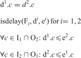
to guarantee that

holds, where

and

are functions defined by the equations:

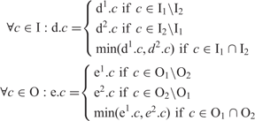
These rules allow us to calculate and prove delays in a modular way for composed systems given delays for their components.

We construct the maximal guaranteed delay b for the feedback loops in a composition. We assume that for all i ∈ {1, 2}

holds and that for all channels c ∈ I₁ ∩ O₂

and for all c ∈ I₂ ∩ O₁

where input delay b is defined as

with

and where we inductively calculate the delays

as follows

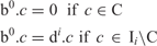
where C is the set of feedback channels

The delays b^{k + 1} are defined inductively by

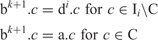
where the delay a: O₁ ∪ O₂ → IN is the maximal numbers such that

holds.

Note that b is the ‘least fixpoint’ of the delay function.

The construction uses as its basis the compositionality of the calculus.

5.9. Deducing delay equations

We consider a network N with interface behavior F_N with a number of systems as data flow nodes. Let C be the set of all channels in the net N. We want to calculate a delay profile

With every system behavior F in the network we may associate a function

for every output channel c defined by

This equation calculates the maximal guaranteed delay for channel c given the delays d.c ₁, …, d.c _n for the input channels of F.

To calculate for every channel c in the network its delay d.c we associate with every node and every output channel c of one of the nodes F the equation

For the input channels c we assume

We get an equation for each channel c ∈ C. It is easy to show that the functions gdel_F(c) are all monotonic. Therefore, there exists a least fixpoint d for the equations which is the delay profile.

6.1. Strong causality and compositionality of coarsening

In this section we study cases that guarantee the validity of the equation

As we will explain in Section 9.3, coarsening is fundamental for a flexible timing of large systems architectures.

That this equation does not hold, in general, can immediately be concluded from our discussion of causal and not causal fixpoints.

Theorem: Let F₁ and F₂ be behaviors that can be composed (according to consistent channel naming and typing); then the following equation holds

Proof: By definition, the statement (let all definitions be as in the definition of ⊗)

stands for: there exists a history z for all channels in I₁, I₂, O₁, and O₂ such that y = z|O and

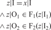
Now let us assume y′ ∈ COA(F₁ ⊗ F₂, n).x′; then there exists y ∈ (F₁ ⊗ F₂).x such that x′ = COA(n).x and y′ = COA(n).y and there exists z such that y = z|O and

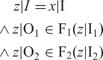
From this, we get with z′ = COA(n).z:

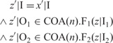
Since by definition of COA(n) we get

we get

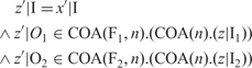
and finally

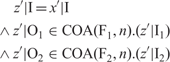
which proves that

and thus that

This completes the proof.

The theorem shows that

is a refinement of

The converse statement is not true, in general. It holds only if both F₁ and F₂ are not sensitive to the finer timing.

Theorem: Let n > 1 hold. Assume for i = 1, 2 that we have (for all x, x )

and that delay(F_i, n) holds, then we get:

Proof: The proof that under the given assumptions the formula holds uses the stepwise construction of the history z such that

for any given z′ with

with z′ = COA(n).z. Note that y′ ∈ (COA(F₁, n) ⊗ COA(F₂, n)).x′ iff such a history z′ exists with y′ = z′|O. From the existence of z we can conclude y′ = COA(n).z and y′ ∈ COA(F₁ ⊗ F₂, n).

This construction is inductive and uses the fact that the behaviors are strongly causal. Since delay(F_i, n) holds for i = 1, 2, we can conclude that COA(F_i, n) is strongly causal for i = 1, 2.

By the assumption we get for any history d and b such that

with the history a ∈ O_i → (M*)^n*k specified by

and

that there exists a history a′ ∈ O_i → (M*)^n*(k+1) such that

and

Now let

hold; then there exists a history z′ such that y′ = z′|O and

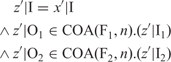
We construct a history z such that z′ = COA(n).z holds and

inductively as follows: since delay(F_i, n) holds there exists a history

such that z′↓1 = COA(n).z ⁽⁰⁾ and for every z′′ we have (for i = 1, 2)

This follows from the fact that F_i.a↓n = F_i.b↓n for all a, b since delay(F_i, n) holds and therefore

Given z ^(k) ∈ C → (M*)^{n*(k + 1)} where

and

there exists z ^{(k + 1)} ∈ C → (M*)^{n*(k + 2)} such that

This follows from the fact that

For all a, b since delay(F_i, n) holds and therefore

By induction we get for all k:

and

and thus for z with z↓(n*(k+1)) = z ^(k) for all k

and

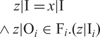
This proves that

and thus concludes the proof.

Moreover, if a component is time independent, then we have the validity of the following equation:

However, in contrast to problems when coarsening behaviors, the equation

does always hold, as long as F₁ and F₂ are strongly causal.

8.1. Strongly and weakly causal behaviors

In this section we explore possibilities to identify causal fixpoints for weakly causal behaviors. In fact, there is a natural implicit notion of strong causality that applies even for weakly causal systems.

Definition:Causality

An I/O-behavior (that is weakly causal)

is called causal (properly timeable), if there exists a number n ∈ IN and a strongly causal function

such that F = COA(F′, n).

In other words, in the definition above, F is a causal function that is weakly causal and can be understood as an abstraction (by time coarsening) of some strongly causal function F′. The critical question, however, is whether such a strongly causal function is unique and thus leads to a canonical construction of causal fixpoints.

Every fixpoint of the strongly causal function F′ is a fixpoint of the weakly causal function F since

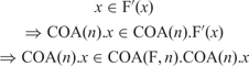
Given a weakly causal function F the existence of a strongly causal function F′ such that F is an abstraction of F′ does not really help, however, to separate faithful fixpoints from causal loops. There are cases where there are several choices of strongly causal behaviors F′, say F₁′ and F₂′, such that some fixpoints of F are causal for F₁′ but not for F₂′. This leads to the following fact: time abstractions may lose the notion of strong causality leading to models where we cannot distinguish causal from non-causal fixpoints. The information loss by time abstraction is therefore critical, in general, and does not allow any longer distinguishing causal from non-causal fixpoints.

We illustrate this problem by an example. First we show an example where weak causality works.

Example. Identity

Consider again some identity function F with . We can prove that fix F is the empty stream. The proof is essentially the same as the one given above. We assume that there is a strongly causal function and that every causal fixpoint of F corresponds to a fixpoint of the strongly causal function. This way we easily deduce for every fixpoint.

This shows that the assumption of strong causality leads to proof of principles for systems with feedback loops. But the assumption does not allow us to rule out non-causal fixpoints in a canonical way. Only strong causality guarantees that all fixpoints are causal and that we do not have fixpoints for which we do not know whether they are causal or not.

Finally, to demonstrate the significance of strong causality let us look at a slightly trickier example. We consider a function F with the following characteristic behavior:

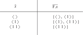
Depending on the structure of its timing the history x with can be a causal fixpoint or not (here 〈〈〉〉^∞ denotes the infinite stream with empty sequences of messages in each time interval) depending on the actual definition of F. The following table shows a particular version of F:

In this case F is (more precisely, can be extended to) a strongly causal function and the stream 〈1〉^∧〈〈〉〉^∞ is a causal fixpoint.

Now consider the strongly causal function F′ with the following characteristic behavior

In this case 〈1〉^∧〈〈〉〉^∞ is not a causally correct fixpoint of F′, although

do coincide. In such a case, the timing of the output is essential for determining the causality of fixpoints and therefore for determining which of the fixpoints are causal.

9.1. Causality and composition

Given a set of specified components we get for each component

with the relational specification (‘specifying assertion’) for y ∈ F.x in the form of a predicate P:

by imposing causality the logical weakest specification Pc that fulfills the following equation

This way we can add the requirement of strong causality to every specification to get a strongly causal specification. Note, that the specification may become inconsistent if the original specification contradicts the notion of strong causality. As is well-known (and straightforward to prove), if we compose strongly causal systems we get again strongly causal systems.

9.2. Composition and coarsening time

If we compose strongly causal systems, then their time delays accumulate. For instance, if each component has a time delay of at most one, then computing the time delay of a composed system is the result of calculating the minimal number of delays of components on the shortest path from an input to an output channel. This allows us to calculate delays in architectures of composed systems. But sometimes we may be interested in a more abstract view on the function computed by an architecture.

If we work with a component F with delay k, we easily construct a strongly causal component of delay one by the component

This construction can be understood as a way to abstract from the finer time scale used inside for the sub-systems of a system to a coarser time scale outside of the system. We may speak of a macro/micro time scale. As long as we are not interested in the fine-grained notion of time, such an abstraction is certainly appropriate. It is the best abstraction maintaining crucial notions such as causal fixpoints and ways to reason about them.

9.3. Local timing

The flexibility of our timing calculus can be seen in the following by demonstrating how we can work with local timing and local clocks.

For each subsystem (subcomponent) of a network we can introduce a local time and a local time granularity. This idea is demonstrated by a simple example.

Example: Architecture with local Time Granularities

The following expression

denotes a system with a subsystem

This way we get a system with different local time scales where each time scale can be chosen fine enough for each of the components locally to guarantee strong causality of each of its subcomponents such that all local computations are captured on the right level of time granularity. The components operate locally on a higher frequency. Since delays accumulate in a system the larger components composed of many subcomponents show typically larger delays such that we can choose coarser time granularity for them without losing strong causality.

Figure 12 shows an informal example of a complex system composed of three subsystems, each of which is composed of four components. For each of the subsystems we may select local proprietary time granularity.

Figure 12

Hierarchical architectures of components with different time scales.

9.4. Multiplexing of the components of a network on one CPU

In general, we cannot expect that each dedicated node in a data flow net always runs on its own CPU. We rather expect that a complete net or sub-net of components is executed on one CPU. Then the multiplexing of the components, which may be running at different speeds, have to be mapped by a scheduling onto the CPU cycles.

9.5. Avoiding causal loops

In the following, we finally discuss the problem of causal loops. We show how we can add strong causality as a property to specifications to reason about feedback loops.

Example: Interface specification

Consider the following specification of a component that copies its input on channel x on both of its output channels y and r.

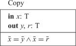
Strong causality as an assumption on the specification Copy allows us to conclude in addition to the specifying assertion the following property:

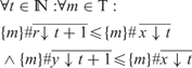
where M x denotes the number of copies of messages in the set that occur in x. Another example is the specification of component Repeater, which repeats each of its inputs infinitely often. Its specification reads as follows:

Repeater

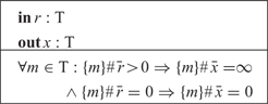
Strong causality allows us to conclude in addition to the specifying assertion the following property

Now let us compose the two components into the composed system characterized by the term

as shown in Figure 13. We get a system that forms a feedback loop. If we want to reason about the composed system, we have to refer to the assumption of strong causality to reason about the system in a way where we avoid causal loops.

Figure 13

Composition repeater ⊗ copy.

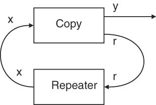
Without strong causality arguments we get the following formula:

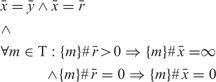
which simplifies to

which indicates for the output y of the network only

With strong causality arguments we get in addition the assertion

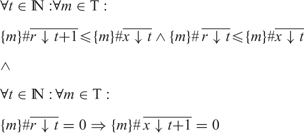
that allows us to conclude (by a simple inductive argument) the validity of the following formula

which cannot be concluded without strong causality.