2.1 Governing equations

The immediate neighbourhood of a given droplet is characterized by a local value of the supersaturation field $s=p/p_{s}-1$ (where $p$ is the vapour partial pressure and $p_{s}$ is the saturation pressure), which induces the growth of its squared radius $r^{2}$ , i.e. the droplet surface area:

The coefficient $a_{3}$ is assumed to be constant, i.e. the small temperature dependence is neglected. It is here understood that the time scale associated with the establishment of vapour diffusion is faster than the external time scales, especially the smallest scale of turbulence, the Kolmogorov scale $\unicode[STIX]{x1D70F}_{\unicode[STIX]{x1D702}}$ (see, e.g., Pruppacher & Klett Reference Pruppacher and Klett1997; Vaillancourt et al. Reference Vaillancourt, Yau and Grabowski2001, for a detailed derivation). This approximation might become invalid in some highly turbulent environments encountered in technical applications where $\unicode[STIX]{x1D70F}_{\unicode[STIX]{x1D702}}$ can be very small. Additionally, it is assumed that the droplet volume loading is small enough to ensure no overlap between the diffusion regions of different droplets. Finally, curvature and salinity effects relevant for the activation and affecting the growth of very small droplets are neglected (Celani et al. Reference Celani, Mazzino and Tizzi2008). Instead, we assume that a completely evaporated droplet is simply reactivated if it is located in a region with positive supersaturation playing the role of a condensation nucleus that stays in the system. We show in § 4 that the specific type of boundary condition imposed at $r=0$ is not important for the large-value tail of the droplet size distribution, i.e. far away from the zero-size boundary.

The growing and shrinking droplets are transported by a turbulent gas velocity $\boldsymbol{u}$ according to the Stokes drag law

where $\boldsymbol{x}$ and $\boldsymbol{v}$ are the particle position and velocity, $\unicode[STIX]{x1D70F}_{d}=2\unicode[STIX]{x1D70C}_{d}r^{2}/(9\unicode[STIX]{x1D70C}\unicode[STIX]{x1D708})$ is the droplet response time, $\unicode[STIX]{x1D70C}_{d}$ is its mass density, and $\unicode[STIX]{x1D70C}$ and $\unicode[STIX]{x1D708}$ are the gas mass density and kinematic viscosity respectively. The Stokes drag approximation is valid for very small and heavy liquid droplets. The droplet radius $r$ has to be smaller than the smallest scale of turbulence, the Kolmogorov dissipative scale $\unicode[STIX]{x1D702}=\unicode[STIX]{x1D708}^{3/4}/\unicode[STIX]{x1D700}^{1/4}$ , where $\unicode[STIX]{x1D700}$ is the mean kinetic energy dissipation rate of the turbulent gas flow. Although the liquid to gas density ratio $\unicode[STIX]{x1D70C}_{d}/\unicode[STIX]{x1D70C}$ is typically large, the droplet size and therewith its mass are typically small enough for gravitational acceleration to be neglected. A posteriori we know that in our parameter range the droplet motion is practically identical to tracer motion as the droplet response time stays negligibly small. Furthermore, for the smallest droplets Brownian motion might become important.

The gas velocity $\boldsymbol{u}$ evolves according to the incompressible Navier–Stokes equation

where $p$ is the pressure and $\unicode[STIX]{x1D719}_{u}$ is a large-scale forcing, which maintains turbulence in a developed regime. Mixing with the environment at the boundaries, often called entrainment and detrainment, is neglected. Additionally, as for the droplets, we neglect temperature and gravity effects, including buoyancy. This might be the strongest approximation, as latent heat release upon condensation is often a strong source for natural moist convection. However, without the anisotropies introduced by buoyancy and edge effects, we generate a homogeneous and isotropic turbulent flow. This drastically simplifies the statistics and their interpretation, and thus motivated us to use these approximations as a first step. As a matter of fact, we will show that some of our results are similar to those of Celani et al. (Reference Celani, Mazzino, Seminara and Tizzi2007), who accounted for the temperature field and buoyancy effects.

Since thermal effects are neglected, it is not necessary to treat the temperature and vapour fields separately. Instead, the supersaturation $s$ can be modelled as a passive scalar coupled to the Lagrangian particles,

where $\unicode[STIX]{x1D705}$ is the molecular diffusivity of the vapour inside the gas. The second term on the right-hand side accounts for the local change in supersaturation due to the presence of $N$ droplets. There, $\boldsymbol{x}_{i}$ denotes the position of the $i$ th droplet and the coefficient $a_{2}$ accounts for the change in both vapour mass and temperature due to the condensation or evaporation. We assume again that the temperature dependence of $a_{2}$ is negligible. There are two common choices for the forcing term $\unicode[STIX]{x1D719}_{s}$ . The first one, often used in experiments on passive scalars, is to impose a mean gradient (Warhaft Reference Warhaft2000). In atmospheric conditions, there is often a vertical temperature gradient, so that updraughts increase the supersaturation (Squires Reference Squires1952; Twomey Reference Twomey1959). Hence, the DNS studies in the context of cloud physics (see § 1) considered $\unicode[STIX]{x1D719}_{s}=\boldsymbol{u}\boldsymbol{\cdot }(0,0,a_{1})$ , where $a_{1}$ is a constant that depends weakly on temperature. If $a_{1}$ is assumed to be constant, this forcing is just a special form of the mean gradient forcing. The second choice, more commonly used in the physics community and in numerical simulations on the advection of passive scalars by a turbulent flow, is to also force the supersaturation field by a large-scale forcing. The properties of the supersaturation field without droplets, which is then a passive scalar, are thus well known. Even if this has been recently questioned by Gotoh & Watanabe (Reference Gotoh and Watanabe2015), one expects such properties to not depend on the specific form of forcing and to display some universality. For instance, coherent structures are present at all length scales, separated by regions where the field undergoes significant fluctuations, the so-called fronts associated with very sharp gradients (Celani et al. Reference Celani, Lanotte, Mazzino and Vergassola2001). If there is no mean forcing input ( $\int _{\unicode[STIX]{x1D710}}\unicode[STIX]{x1D719}_{s}\,\text{d}^{3}x=0$ ), the mean value of supersaturation remains constant. Then, the system (2.1)–(2.4) conserves the global mass of liquid and vapour,

Similar mass balances have been proven to be useful to obtain analytical results (Pinsky et al. Reference Pinsky, Mazin, Korolev and Khain2013; Devenish, Furtado & Thomson Reference Devenish, Furtado and Thomson2016). Motivated by our idea to concentrate on the influence of turbulent mixing, we choose here to use a large-scale forcing for $\unicode[STIX]{x1D719}_{s}$ . We will show in § 6 that we can explain the results of DNS studies with updraught forcing by the outcomes of our simulations. However, in contrast to assuming a mean gradient, our choice ensures the statistical homogeneity and isotropy of the scalar field $s$ , and hence of the droplet sizes.

2.2 Qualitative predictions

In the various systems (see § 1), the physical parameters such as the kinematic viscosity of the gas, the number of droplets and the total amount of liquid and vapour can take very different values. To treat the problem of turbulent condensation as generally as possible, i.e. independently of any specific application, we analyse here dimensionless equations. Thereby, non-dimensional groups are obtained by dimensional analysis that are determining the solutions of the system of differential equations. As long as the assumptions made in the previous subsection are not violated, the solutions we obtain can be applied to a specific application, once they have been rescaled together with time and length scales using the specific dimensional parameters. Non-dimensional quantities are always written in capital letters to distinguish them from the dimensional quantities written in lowercase.

The turbulent fluctuations of supersaturation along droplet trajectories are essentially correlated over the large scales, because to leading order, droplets are Lagrangian objects. We thus decide to use as a reference length the large scale $l_{0}=u_{rms}^{3}/\unicode[STIX]{x1D700}$ , where $u_{rms}$ is the root-mean-square (r.m.s.) velocity, and as a reference time the large-eddy turnover time $t_{0}=l_{0}/u_{rms}$ .

Application of this to the Navier–Stokes equations (2.3) leads to the Reynolds number

which is the ratio of the viscous mixing time scale to the turbulent advection time scale. In principle, we want the Reynolds number as large as possible in order to have a large separation between the forcing and dissipation scales. However, the computational effort increases with the resolution, such that most of our simulations will be conducted at $Re=2100$ .

The droplet equation of motion (2.2) leads to introduce the large-scale Stokes number

A priori, the droplet sizes evolve with time, and so do the Stokes numbers. Motivated by the global mass balance (2.5), we choose here and in the following to use the droplet mass averaged over the whole population as the typical size $\bar{r}=f(t)$ , namely $\bar{r}=\langle r(t)^{3}\rangle ^{1/3}$ . As the droplets are typically small, we expect the Stokes number to be small, so that inertia effects, such as clustering, are weak even on the smallest scales.

The supersaturation equation (2.4) provides two time scale ratios: the Schmidt number,

which we only consider to be one, and the time scale of change in supersaturation due to condensation,

which is obtained from a spatial average and depends on both the characteristic radius $\bar{r}$ and the droplet number density $n_{d}$ .

The supersaturation diffusion–advection equation (2.4) is linear and hence the proper choice for the reference value of $s$ is not straightforward. We select its standard deviation $s_{rms}$ in the absence of droplets. From the droplet growth equation (2.1), a time scale arises, which we call hereafter the condensation time scale,

This condensation time scale did not receive much attention in recent DNS studies of homogeneous condensation (Vaillancourt et al. Reference Vaillancourt, Yau, Bartello and Grabowski2002; Celani et al. Reference Celani, Falkovich, Mazzino and Seminara2005; Lanotte et al. Reference Lanotte, Seminara and Toschi2009; Sardina et al. Reference Sardina, Picano, Brandt and Caballero2015). However, it is known and used in the context of mixing of sub- and supersaturated regions. Based on the notation in reacting flows, a Damköhler number is constructed to compare the turbulent mixing time scale with the time for phase change (Devenish et al. Reference Devenish, Bartello, Brenguier, Collins, Grabowski, IJzermans, Malinowski, Reeks, Vassilicos and Wang2012). In this sense, the dimensionless quantities defined in (2.9) and (2.10) can be seen as inverse Damköhler numbers. This raises a question about the relevant time scales that characterize the system. From their DNS results, Kumar et al. (Reference Kumar, Janetzko, Schumacher and Shaw2012) concluded that the Damköhler number based on the supersaturation time scale is the relevant one. However, Lehmann, Siebert & Shaw (Reference Lehmann, Siebert and Shaw2009) argued that the time scale of the coupled system might be very different from both the condensation and supersaturation time scales.

We give here some preliminary heuristic arguments on possible asymptotic behaviour of the system. Let us consider the supersaturation equation (2.4). If $\unicode[STIX]{x1D70F}_{s}$ is very large, the influence of the particle on the supersaturation field is small, i.e. its evolution is dominated by turbulent mixing characterized by the time scale $t_{0}$ . Conversely, if this supersaturation time scale is very small, the condensation or evaporation of droplets dominates the variations of $s$ , and the characteristic time scale for the supersaturation evolution is $\unicode[STIX]{x1D70F}_{s}$ . The supersaturation field thus changes on a time scale given by the minimum of $t_{0}$ and $\unicode[STIX]{x1D70F}_{s}$ . Assume now that the condensation time scale $\unicode[STIX]{x1D70F}_{c}$ is much larger than the minimum of $t_{0}$ and $\unicode[STIX]{x1D70F}_{s}$ , meaning that the droplet sizes change slowly compared with the supersaturation field. This was implicitly assumed in mean-field models and corresponds to the homogeneous case (small Damköhler number) in the context of chemical reactions. In this case, individual droplets experience a rapidly changing supersaturation, which to leading order can be approximated as a random white noise. From (2.1), one infers that their surface area $r^{2}$ follows a Brownian motion. This implies that the standard deviation of the droplet surface $\unicode[STIX]{x1D70E}_{r^{2}}$ , which gives a measure of the spectral broadening, evolves as $\propto \sqrt{t}$ . Conversely, if we now consider that $\unicode[STIX]{x1D70F}_{c}$ is much smaller than the minimum of $t_{0}$ and $\unicode[STIX]{x1D70F}_{s}$ , the droplet sizes change faster than the supersaturation value along their trajectories. We are then in the inhomogeneous limit, where more complex dynamics can be expected. Droplets experience a quasiconstant supersaturation value for a long time and change their sizes rapidly. This could lead to both very large droplets and complete evaporation. We thus expect a very broad droplet size spectrum in this case.

Table 1.

Parameters of the numerical simulations for the turbulent gas flow with respect to the large-scale values of the intermediate-resolution case denoted as $l_{\ast }$ and $t_{\ast }$ : $N_{x}^{3}$ , number of spatial collocation points; $\unicode[STIX]{x1D708}$ , kinematic viscosity; $\unicode[STIX]{x1D702}=\unicode[STIX]{x1D708}^{3/4}/\unicode[STIX]{x1D700}^{1/4}$ , Kolmogorov dissipative scale; $\unicode[STIX]{x1D70F}_{\unicode[STIX]{x1D702}}=\unicode[STIX]{x1D708}^{1/2}/\unicode[STIX]{x1D700}^{1/2}$ , Kolmogorov time; $u_{rms}$ , r.m.s. velocity; $l_{0}=u_{rms}^{3}/\unicode[STIX]{x1D700}$ , large scale; $t_{0}=u_{rms}^{2}/\unicode[STIX]{x1D700}$ , large-eddy turnover time; $t_{u}$ , integral time scale of the Lagrangian velocity autocorrelation; $t_{s}$ , integral time scale of the Lagrangian scalar autocorrelation; $Re=u_{rms}l_{0}/\unicode[STIX]{x1D708}$ , large-scale Reynolds number; $R_{\unicode[STIX]{x1D706}}=\sqrt{15}u_{rms}^{2}\unicode[STIX]{x1D70F}_{\unicode[STIX]{x1D702}}^{2}/\unicode[STIX]{x1D702}^{2}$ , Taylor microscale Reynolds number.

2.3 Direct numerical simulations

We conduct a series of DNS of the flow and the supersaturation field with the pseudospectral code LaTu (Homann, Dreher & Grauer Reference Homann, Dreher and Grauer2007) in a cubic periodic domain. The gas flow forcing $\unicode[STIX]{x1D719}_{u}$ is chosen to keep constant the energy content of the first two shells of wavenumbers in Fourier space. The supersaturation forcing $\unicode[STIX]{x1D719}_{s}$ is Gaussian white noise in time and is concentrated at wavenumbers with moduli between $1$ and $2.5$ . The various non-dimensional parameters are reported in table 1. Most simulations are performed at a resolution of $512^{3}$ collocation points, corresponding to a Taylor microscale Reynolds number of $R_{\unicode[STIX]{x1D706}}\approx 180$ . The ratio between the largest and smallest time scales is $t_{0}/\unicode[STIX]{x1D70F}_{\unicode[STIX]{x1D702}}\approx 50$ , indicating a sufficient scale separation. Additionally, selected simulations are repeated at decreased ( $256^{3}$ ) and increased ( $1024^{3}$ ) resolutions, corresponding to $R_{\unicode[STIX]{x1D706}}\approx 100$ and $R_{\unicode[STIX]{x1D706}}\approx 320$ respectively, in order to test possible Reynolds-number dependence. We only consider cases where the Schmidt number is unity and the Eulerian mean supersaturation is initially zero. The fields are evolved until a statistical steady state is reached. Then, 10 000 000 equal-sized droplets are randomly released in the domain with a large-scale Stokes number of $St=2.3\times 10^{-5}$ to ensure that particle inertia is initially negligible. These Lagrangian droplets, together with their sizes, are subsequently integrated according to (2.1) and (2.2) using a tricubic interpolation of the gas velocity and of the supersaturation value at the particle position. The backreaction of the droplets onto the supersaturation field in (2.4) is performed by linear extrapolation to the nearest collocation points.

Figure 1.

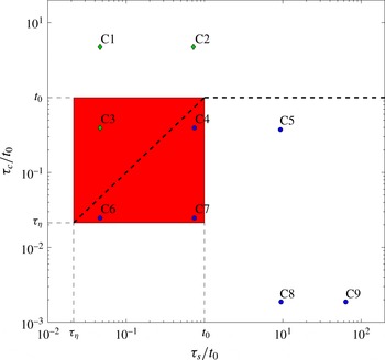
Plot showing the parameter space explored by DNS as labelled points in terms of the condensation time scale $\unicode[STIX]{x1D70F}_{c}$ and the supersaturation time scale $\unicode[STIX]{x1D70F}_{s}$ . The red area spans from the Kolmogorov time scale $\unicode[STIX]{x1D70F}_{\unicode[STIX]{x1D702}}$ to the large-eddy turnover time $t_{0}$ to indicate the turbulent inertial range. The thick dashed line separates the region above in which $\unicode[STIX]{x1D70F}_{c}>\min (\unicode[STIX]{x1D70F}_{s},t_{0})$ with green diamonds from the region with $\unicode[STIX]{x1D70F}_{c}<\min (\unicode[STIX]{x1D70F}_{s},t_{0})$ with blue circles.

Table 2.

The parameter space explored by DNS cases C1–C9 in terms of the condensation and supersaturation time scales $\unicode[STIX]{x1D70F}_{c}$ and $\unicode[STIX]{x1D70F}_{s}$ .

The parameter space explored in terms of the condensation and supersaturation time scales $\unicode[STIX]{x1D70F}_{c}$ and $\unicode[STIX]{x1D70F}_{s}$ is visualized in figure 1 and additionally summarized in table 2. Different combinations are chosen in or close to the turbulent inertial range in order to detect possible interferences or resonances between the various physical processes.

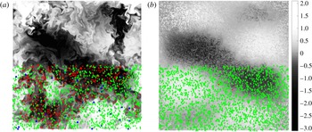
In § 2.2, we anticipated two different asymptotic regimes. For a first impression of these two regimes, we select the cases C3 and C4 for visualization. They feature the same value of the condensation time scale $\unicode[STIX]{x1D70F}_{c}<t_{0}$ , but C4 has a larger value of the supersaturation time scale $\unicode[STIX]{x1D70F}_{s}<t_{0}$ , such that we expect to obtain for these instances the two different asymptotic regimes. Two-dimensional cuts of the two supersaturation fields are shown in figure 2. Figure 2(a) shows the case C4 where $\unicode[STIX]{x1D70F}_{c}<\unicode[STIX]{x1D70F}_{s}<t_{0}$ . The supersaturation field clearly looks like a turbulent passive scalar as described in § 2.1 (see Warhaft Reference Warhaft2000, for a review). Hence, the influence of the droplets is practically unnoticeable, except globally as the spatial average of $s$ is negative. In figure 2(b), the case C3, where $\unicode[STIX]{x1D70F}_{s}<\unicode[STIX]{x1D70F}_{c}<t_{0}$ , is represented and displays a completely different behaviour. The local fluctuations of $s$ are strongly reduced at both positive and negative values. Large-scale structures still exist, but intermediate-scale variations are smoothed out by the droplet–vapour exchange. At fine scales, the influence of the individual droplets can be recognized. Their positions are superimposed on the lower half of figure 2. There are very few completely evaporated droplets, but no droplet that has doubled its surface area after $3.1t_{0}$ . For comparison, in the case C4 (figure 2 a), there are large droplets and a huge portion of evaporated droplets can be found in regions with a negative supersaturation.

Figure 2.

Slice of thickness $0.4\unicode[STIX]{x1D702}$ through the 3D supersaturation field at $t=3.1t_{0}$ : (a) case C4, (b) case C3. The value of $s/s_{rms}$ is given as a greyscale contour plot. Additionally, the droplets are superpositioned in the lower half. Their size is increased for better visibility; their colour indicates their real size: red stars are for $r^{2}=0$ , green diamonds for the intermediate sizes ( $0<r^{2}<2\langle r^{2}\rangle$ ) and blue circles for $r^{2}>2\langle r^{2}\rangle$ .

3.1 Derivation

We are interested in the behaviour of the joint distribution of $r^{2}$ and $s$ along droplet trajectories at large times. As the large-scale Stokes number is small, we assume that droplet inertia can be neglected. Following ideas borrowed from PDF modelling of turbulent mixing (see Pope Reference Pope2000), we assume that along droplet trajectories, the variations of supersaturation due to diffusion and forcing can be approximated at large times by a Langevin (Ornstein–Uhlenbeck) process. The correlation time should then be the integral time scale of the Lagrangian scalar autocorrelation $t_{s}$ , and the drift the (time-dependent) Eulerian average of the supersaturation field $\langle s\rangle _{E}$ . When taking into account the variation of supersaturation due to condensation or evaporation of the droplet from (2.4), this leads to modelling the evolution of $s$ along droplets as

where $\unicode[STIX]{x1D709}$ is the standard white noise. Hence, it should be noted that this evolution equation is a stochastic differential equation, which has to be taken into account when, e.g., computing the moments of $s$ . The evolution equation is, of course, supplemented by (2.1) to account for the time variations of the droplet radius $r$ . This modelling involves the Eulerian average $\langle s\rangle _{E}$ of the supersaturation field, which is not directly given by a Lagrangian approach but can be inferred from the global mass conservation of liquid and vapour. We indeed have from (2.5) combined with (2.9) and (2.10)

The Eulerian averaged supersaturation is thus a global quantity that depends on the full distribution of $r$ . In that sense, the system is not closed at the level of a single droplet, and the associated Fokker–Planck equation is an integro-differential equation. Because of this, our model differs from that proposed by Paoli & Shariff (Reference Paoli and Shariff2009). They have indeed used the Lagrangian mean of $s$ instead of the Eulerian one. Additionally, we want to emphasize that the supersaturation along trajectories is correlated over times corresponding to the Lagrangian integral time scale of the scalar $t_{s}$ . Table 1 shows, in agreement with Yeung (Reference Yeung2001), that $t_{s}$ generally differs from the large-eddy turnover time $t_{0}$ used by Paoli & Shariff (Reference Paoli and Shariff2009) and the Lagrangian integral time scale of the velocity $t_{u}$ used by Sardina et al. (Reference Sardina, Picano, Brandt and Caballero2015).

To single out the relevant parameters, we next rescale time $t$ by $t_{s}$ , the supersaturation $s$ by $s_{rms}$ and the droplet radius $r$ by $\bar{r}\sqrt{t_{s}/\unicode[STIX]{x1D70F}_{c}}=\sqrt{2a_{3}s_{rms}t_{s}}$ . The model then reads

The evolution depends upon two parameters: the global mass

and the constant $A$ , which determines how strongly the evolution of $R$ couples back to the evolution of $S$ . It is given by the two time scales $\unicode[STIX]{x1D70F}_{c}$ and $\unicode[STIX]{x1D70F}_{s}$ , namely

To provide evidence that $t_{s}$ is the correct correlation time, we conduct DNS at various resolutions, i.e. varying the Reynolds number, while at the same time we keep the dimensionless parameters $\unicode[STIX]{x1D70F}_{c}/t_{s}$ and $\unicode[STIX]{x1D70F}_{s}/t_{s}$ constant. 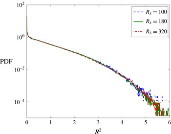As depicted in table 1, these parameters would differ by 20 or 25 % in this Reynolds number range if $t_{0}$ or $t_{u}$ had been used instead. Figure 3 shows the PDF of the normalized droplet surface area $R^{2}$ for the three different Reynolds numbers at a specific time $T$ . The collapse of the distribution confirms the role of large-scale mixing and emphasizes the choice of $t_{s}$ as a reference time scale. As $\unicode[STIX]{x1D702}$ decreases with the Reynolds number at fixed $l_{0}$ , we also decreased $r$ accordingly to stay in the Stokes drag limit (see § 2.1). We kept the particle volume loading $n_{d}$ constant; hence, the number of particles increases with the Reynolds number. That is why the $R^{2}$ tail contains less statistical noise at higher Reynolds number. Still, by normalizing with the Reynolds-number-dependent values of $t_{s}$ and $s_{rms}$ the PDF of $R^{2}\left(T\right)$ is collapsing, i.e. if there is any Reynolds-number dependence at all it is only very weak.

Figure 3.

Comparison of three DNS runs with increasing resolution and therewith Taylor-scale-based Reynolds number but the same parameters $\unicode[STIX]{x1D70F}_{c}/t_{s}$ and $\unicode[STIX]{x1D70F}_{s}/t_{s}$ , namely those of case C8, by means of the PDF of $R^{2}$ at $t=6.2~t_{s}$ : blue, $256^{3}$ at $R_{\unicode[STIX]{x1D706}}=100$ ; green, $512^{3}$ at $R_{\unicode[STIX]{x1D706}}=180$ ; red, $1024^{3}$ at $R_{\unicode[STIX]{x1D706}}=320$ .

The nonlinear integro-differential stochastic system (3.3) is much simpler than the original governing system of partial-differential equations, but still too complex to be solved analytically. As done by Paoli & Shariff (Reference Paoli and Shariff2009), the evolution of the moments can be written down from the model equations (3.3):

This is an unclosed hierarchy of equations and can only be solved if additional closure assumptions are made. However, it is possible to understand the system dynamics qualitatively. A typical trajectory in the phase space is shown in figure 4. Due to the noise term, the supersaturation tends to make Brownian excursions. For negative values of $S$ , the droplet shrinks, while for positive values, the droplet grows. The drift term prevents runaway excursions to $s=\pm \infty$ . 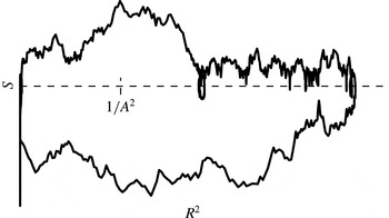It should be noted that the nonlinear coupling term $-ARS$ is dominant for large droplets, $R^{2}\gg 1/A^{2}$ . Thereby, the larger the droplet is, the faster a positive $S$ is reduced to zero, so that large droplets can grow only on very short time scales. Conversely, an evaporating droplet is less and less effective in pushing its negative supersaturation back to zero and thus has longer and longer time to shrink. Due to this bias, it seems reasonable to assume that a droplet cannot grow infinitely large. In the opposite limit, when a droplet completely evaporates (reaches $R=0$ ), the dynamics of $S$ decouples from $R$ and the droplet will start to grow only once $S$ becomes positive, reinitializing the full process again. There is thus a loss of memory of the previous growth history. Bounded excursions, together with the recurrent memory losses, suggest that, at long time, the system should reach a statistical stationary state independent of its initial condition.

Figure 4.

Example of a typical dynamic in the $R^{2}$ – $S$ phase space.

3.2 Comparison with DNS

We perform Monte-Carlo (MC) simulations of the system (3.3) for the same parameters as in the DNS cases C3 and C4 shown in figure 2. Thereby, the parameters $A$  (3.5) and $\langle W\rangle$  (3.4) are calculated from the DNS initial conditions. In particular, $t_{s}$ and $s_{rms}$ are measured from the initial supersaturation field as the afterwards released droplets change its properties. The parameters $A$ and $\langle W\rangle$ both depend on $s_{rms}$ ; hence, the model is sensitive to the value of $s_{rms}$ . The MC simulations allow us to simulate the system for much longer times than the DNS.

Figure 5.

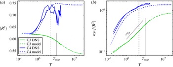
Comparison of the DNS (solid lines) with the results of the stochastic model (dashed lines) for the cases C3 (green) and C4 (blue). It should be noted that for case C4 two independent DNS runs are shown. (a) Time evolution of the mean droplet surface area $\langle R^{2}\rangle$ . (b) Time evolution of the relative standard deviation of the droplet surface area $\unicode[STIX]{x1D70E}_{R}^{2}/\langle R^{2}\rangle$ . The vertical black solid line marks $T_{evap}$ for C3, at which $\unicode[STIX]{x1D70E}_{R}^{2}/\langle R^{2}\rangle$ is predicted to start deviating from the $t^{1/2}$ behaviour (see § 2.2 for the preliminary heuristic arguments and § 5.1 for a detailed derivation of (5.3)). The vertical black dashed line marks the time of the snapshots shown in figure 2.

The evolution of $\langle R^{2}\rangle$ is shown in figure 5(a). In the case C3, the mean value of $R^{2}$ for both the DNS and the model first remains relatively constant and then even decreases. In contrast, for the case C4, the average of $R^{2}$ increases substantially before converging to a constant value. In this case, the model lags a little bit behind the DNS. Additionally, the final value seems to be a few per cent higher, although this is not unambiguous as the DNS value fluctuates strongly. That is why we have represented two different realizations of the full DNS C4 in figure 5. Given the large amplitude of the variations between these two runs and of the fluctuations as a function of time, the deviations from the model could be explainable by a lack of ensemble averaging. While the number of droplets is the same for the DNS and the MC simulation, the supersaturation in DNS is correlated on the large scales, whereas the random increments are independent in the model. Hence, the number of independent realizations is higher in the model. Ensemble averaging of independent DNS realizations would be needed but is computationally too expensive.

Figure 5(b) represents the coefficient of variation of the droplet surface area, namely the relative standard deviation $\unicode[STIX]{x1D70E}_{R}^{2}/\langle R^{2}\rangle$ . In the case C4, it increases first rapidly and then converges, although more slowly than the mean value, to a value close to one. The model values are slightly lower than the DNS values. Nevertheless, for both the model and the DNS, the coefficient of variation is of order one, indicating a very broad distribution close to the one given, for instance, by an exponential distribution. For the case C3, the relative standard deviation starts much lower and, for a decade of time, the predicted $t^{1/2}$ power law can be seen in the logarithmic plot. Hence, while the case C4 is already in the steady state in figure 2, C3 is still in the Brownian-motion regime, leading to the very different pictures. However, also in the case C3, the model eventually converges to a constant value, i.e. a steady state is reached at very large times.

To conclude we want to emphasize two points, First, the MC simulations confirm the above reasoning that, at long times, the system converges to a steady state. Hence, the heuristic arguments of § 2.2 actually describe two regimes of the transient system behaviour. Second, the model predictions are representative of the actual dynamics. The simple stochastic model is indeed able to reproduce some results of the DNS surprisingly well. This is unexpected as the turbulence is only modelled trivially and no intermittency or inertia effects are taken into account. The short-time behaviour is perfectly reproduced, while there are deviations for the steady state. However, these deviations are systematic for all DNS runs reported in figure 1 that we have conducted. We will come back to this issue in the next section.

4.1 Model-based analytical predictions

We can find from the equations of the moments (3.6) that in the steady state, the Lagrangian and Eulerian means of the supersaturation coincide, $\langle S\rangle =\langle S\rangle _{E}$ , as all time derivatives are zero and thus the mixed moments $\langle SR^{x}\rangle$ all vanish. The latter can only be fulfilled if the probability density function of the supersaturation $s$ conditioned on any $R>0$ is symmetric around zero. Due to the convergence of the mean droplet mass $\langle R^{3}\rangle$ and of the mean Eulerian supersaturation $\langle S\rangle _{E}$ , the system (3.3) is no longer a stochastic integro-differential equation as it does not involve integrals anymore. Hence, it can be described by its associated stationary Fokker–Planck equation. To reflect the piecewise definition of the stochastic model (3.3), we split the joint probability density $p$ into an atomic contribution $m$ for evaporated droplets and a smooth part $\tilde{p}$ for active droplets,

The stationary Fokker–Planck equation for the active droplets $\tilde{p}(S,R^{2},T\rightarrow \infty )$ can then be written as

Despite the simplifications in the steady state, it is not straightforward to find a general solution because of the nonlinear coupling term $\left(1+AR\right)S$ . Nevertheless, we can predict the shape of the tail of the distribution $p(R^{2})$ of the droplet surface area. Interpreting the surface area $R^{2}$ as position and the supersaturation $S$ as velocity, equation (4.2) is similar to the Fokker–Planck equation associated with Brownian particles subject to a position-dependent drag. In the large-drag limit, the velocity is a fast variable and can be eliminated. Following Sancho, San Miguel & Dürr (Reference Sancho, San Miguel and Dürr1982), an expansion of the nonlinear drag term yields to leading order

This solution is only valid when the term $(1+AR)$ is dominant, i.e. for large droplets with $R^{2}\gg 1/A^{2}$ (see figure 4). One could think of finding another solution for the opposite asymptotic $R^{2}\ll 1/A^{2}$ and then matching the two limiting solutions similarly to the approach in boundary layer theory. However, due to the finite probability of having completely evaporated droplets, see (4.1), and the complicated boundary conditions at $R=0$ , this is a very challenging task. Still, the large-droplet solution (4.3) has global consequences: to have an integrable distribution of large droplets the mean Eulerian supersaturation $\langle S\rangle _{E}$ has to be negative. As seen above, $S$ conditioned on $R>0$ has to be symmetric around zero, such that the mean value of $S$ in the presence of droplets is zero. Hence, only $S$ conditioned on $R=0$ contributes to the negative $\langle S\rangle _{E}$ . Therefore, it follows that the presence of completely evaporated droplets is a prerequisite for reaching the steady state.

Figure 6.

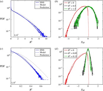
(a,c) Probability density function of $R^{2}$ from the DNS (solid line) and the model (dashed line). The prediction from (4.3) is shown as a thin dashed line. The value $1/A^{2}$ is indicated as a thin solid black line. (b,d) Probability density function of $S$ conditioned on three values of $R^{2}$ . Again, the DNS results are drawn as solid lines while the results from the model are shown as dashed lines. The PDFs are computed for the case C4 (a,b) and the case C6 (c,d).

4.2 Comparison with numerical results

In the following, we show that the theoretical predictions for the PDFs of $R^{2}$ and $S$ not only apply to the model but also to the DNS. In figure 6, the predictions, the MC simulations and the DNS are contrasted by the means of the PDF of $R^{2}$ and the conditioned PDFs of $S$ . For the case C4, which is presented in figure 6(a,b), we know from figure 5 that the model predicts a slightly higher $\langle R^{2}\rangle$ than the DNS. The PDF of $R^{2}$ obtained from the model shows a higher probability for intermediate-size droplets, which leads to this higher mean value. For $R^{2}\gg 1/A^{2}$ , the MC simulation fits the tail prediction (4.3). The tail of the PDF of the DNS is parallel to this prediction, i.e. the shapes match, up to a multiplicative constant. The PDF of the supersaturation $S$ is shown conditioned on the droplet size. For evaporated droplets ( $R^{2}=0$ ), the PDF of $S$ has only negative values. For finite-size droplets, the PDFs are centred at zero and nearly symmetric with practically constant variances, independent of the value of $R^{2}$ on which the PDF is conditioned. The model fits the supersaturation PDFs of the DNS well, although some small deviations can be observed in the negative- $S$ tail.

The trends discussed in the case C4 are representative for all DNS runs that we have conducted and are reported in figure 1. To corroborate this, we also show the data corresponding to the case C6 in figure 6(c,d), which feature smaller $\unicode[STIX]{x1D70F}_{c}$ and $\unicode[STIX]{x1D70F}_{s}$ , i.e. a larger $A$ . The PDF of $R^{2}$ obtained with the model coincides with the prediction at large droplet sizes. Intermediate values of $R$ are less probable in the DNS, but the shape of the tail fits. The PDFs of $S$ are well reproduced. While the PDF of $S$ for evaporated droplets looks very similar to that for the case C4, the active droplets damp the supersaturation more strongly due to the larger coupling parameter $A$ . Because of a smaller variance of $S$ , the droplets are smaller in the case C6 than in the case C4.

4.3 Characterization by the model parameters

In the steady state, the system (3.3) depends only on the two model parameters, namely the coupling parameter $A$ defined in (3.5) and the total mass $\langle W\rangle$ associated with the conservation of liquid and vapour (3.4). In figure 7, the steady state is characterized by the mean drop surface area, its relative standard deviation and the mean Eulerian supersaturation, which are represented as a function of $A$ for various values of $\langle W\rangle$ .

Figure 7.

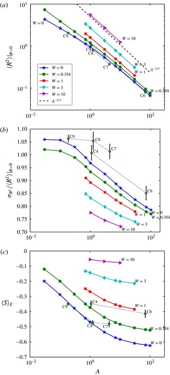
Steady-state values of the mean drop surface area $\langle R^{2}\rangle |_{R>0}$ (a), the relative standard deviation $\unicode[STIX]{x1D70E}_{R^{2}}/\langle R^{2}\rangle |_{R>0}$ (b) and the mean Eulerian supersaturation $\langle S\rangle _{E}$ (c) as a function of $A$ and with the water parameter $\langle W\rangle$ ranging from $0$ to $10$ . For comparison with these model results, the DNS values of the cases C7, C8 and C9 with $\langle W\rangle \sim 0$ and C4 and C6 with $\langle W\rangle \sim 0.354$ are superimposed.

The mean drop surface area $\langle R^{2}\rangle |_{R>0}$ , displayed in figure 7(a), shows approximately a power-law behaviour $\propto A^{-2/3}$ . This can be explained by the conservation of mass (3.4). For large $A$ , the third moment of $R$ corresponding to the mean drop mass has to decrease correspondingly. This argument also explains why $\langle R^{2}\rangle |_{R>0}$ increases with $\langle W\rangle$ . We would like to emphasize the fact that mean-field arguments predict no drop growth for an initially vanishing average supersaturation. In contrast, due to the supersaturation fluctuations, $\langle R^{2}\rangle |_{R>0}$ always converges to a positive non-zero value even for zero total mass in the system.

Following the same scaling arguments, $\langle R^{4}\rangle$ is proportional to $A^{-4/3}$ , such that, to leading order, $\unicode[STIX]{x1D70E}_{R^{2}}/\langle R^{2}\rangle |_{R>0}$ is expected to be constant. However, one finds from figure 7(b) that the size broadening slightly decreases with $A$ . This can be explained by the tail prediction, since $\langle R^{4}\rangle$ depends strongly on the large droplets. For large $A$ , the droplet size distribution has a subexponential tail given by (4.3). Consistently, the relative standard deviation features values smaller than $1$ , which decrease slowly with $A$ . For $A$ going to zero, an exponential distribution would be expected from (4.3), similarly to the case of Brownian motion with reflection. However, the shape prediction is only valid for $(1+AR)$ large, and hence the moments become dominated by the unknown small-drag distribution. The mean drop size increases with $\langle W\rangle$ , so that the tail prediction is valid for a larger portion of the PDF of $R^{2}$ and $\unicode[STIX]{x1D70E}_{R^{2}}/\langle R^{2}\rangle$ becomes smaller.

A negative mean Eulerian supersaturation $\langle S\rangle _{E}$ is a requirement for a steady state (see § 4.1). It should be noted that

Since the PDF of $S$ conditioned on $R=0$ seems to be independent of both $A$ and $\langle W\rangle$ (see figure 6), the value of $\langle S\rangle _{E}$ is directly proportional to the number of evaporated drops. For a small coupling parameter $A$ , the tendency for droplets to be pushed towards $R^{2}=0$ is low, so that most of them are active (see figure 7 c). As $A$ increases, the steady-state fraction of evaporated droplets increases. This leads to more negative contributions to $\langle S\rangle _{E}$ . The mean size $\langle R^{2}\rangle$ increases with $\langle W\rangle$ , and therefore the distance to the zero-size boundary becomes larger. Hence, for larger $\langle W\rangle$ , the probability for evaporated droplets is smaller and $\langle S\rangle _{E}$ is larger, closer to zero.

The DNS statistics are also shown in figure 7. These values are less certain, since, as visible in figure 5, they fluctuate more strongly and the fourth-order moment of $R$ might not be fully converged to its steady-state value at the end of the simulation time of $20t_{s}$ . As expected from figure 5, the DNS cases show lower mean values and higher relative standard deviations. Nevertheless, their scalings are consistent with the model results.

Figure 8.

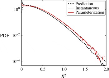
Comparison of the steady-state $R^{2}$ PDF of two MC simulations with different boundary conditions at $R=0$ . Black solid line, instantaneous reactivation as soon as the supersaturation $S$ is positive, according to (2.1); red solid line, activation according to a power-law parameterization in $S$ (Seifert & Beheng Reference Seifert and Beheng2006); black dashed line, prediction given by (4.3).

Finally, to show that the shape of the PDF of $R^{2}$ at large droplet sizes does not depend on the treatment of those with a size close to zero, the model is modified to activate droplets according to a parameterization given by the Köhler–Kelvin theory (see, e.g., Seifert & Beheng Reference Seifert and Beheng2006). In this parameterization, the activation probability behaves as a power law on $S$ . Therefore, the time a droplet spends at $R=0$ until it is reactivated is increased. Hence, the number of evaporated drops in the steady state increases. However, as can be seen in figure 8, the dynamics of large drops far away from the boundary is practically unaffected. This is consistent with the findings of Celani et al. (Reference Celani, Mazzino and Tizzi2008) (see § 1).

5.1 Short-time behaviour

At short times, the evolution of the system still depends on the initial conditions for $S$ and $R$ . We exemplarily explain the short-time behaviour of (3.3) by concentrating on the DNS settings with a normally distributed supersaturation $S\sim {\mathcal{N}}(0,1)$ , where ${\mathcal{N}}(\unicode[STIX]{x1D707},\unicode[STIX]{x1D70E}^{2})$ denotes a normal distribution with mean $\unicode[STIX]{x1D707}$ and standard deviation $\unicode[STIX]{x1D70E}$ , and a monodisperse drop spectrum $\unicode[STIX]{x1D6FF}(R-R_{0})$ . Let us assume that, at short times, the mean droplet mass $\langle R^{3}\rangle$ and the coupling $(1+AR)$ remain approximately constant. The second assumption might seem a bit crude as we are interested in the evolution of the individual radii $R$ . However, turbulent condensation models frequently assume that $\unicode[STIX]{x1D70F}_{s}\bar{r}/r$ is constant, equal to $\langle \unicode[STIX]{x1D70F}_{s}\rangle$ , in order to obtain analytical solutions (see, e.g., Field et al. Reference Field, Hill, Furtado and Korolev2014; Sardina et al. Reference Sardina, Picano, Brandt and Caballero2015). This can be justified globally, as the assumption of constant $\langle R^{3}\rangle$ implies $\langle SR\rangle =0$ ; see (3.6a ). Under such approximations, the evolution of $S$ greatly simplifies: equation (3.3b ) loses its dependence on an integral quantity ( $\langle S\rangle _{E}\approx 0$ ), as well as its nonlinearity ( $AR\approx \text{const.}$ ). Hence, the dynamics of $S$ is independent of $R$ and follows a standard Ornstein–Uhlenbeck process, where $R$ is just the time integration of this process. Therefore, the distributions of $S$ and $R$ are Gaussian and are fully determined by their first two moments. Using (3.6), the distributions of $S$ and $R^{2}$ can be straightforwardly written as

with

where we have used the assumptions that $(1+AR)$ and $\langle \unicode[STIX]{x1D70F}_{s}\rangle$ are constant.

Figure 9.

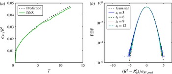
Short-time behaviour of the DNS in the case C1. (a) Relative standard deviation $\unicode[STIX]{x1D70E}_{R^{2}}/\langle R^{2}\rangle$ as a function of time (solid line), in comparison with the prediction of (5.1b ) (dashed line). (b) The PDF of $R^{2}$ standardized by the initial mean value $\bar{R}_{0}^{2}$ and the standard deviation $\unicode[STIX]{x1D70E}_{R^{2},pred}$ predicted by (5.1b ) at different times (solid lines) and in comparison with a standard Gaussian distribution (dashed line).

These predictions are compared in figure 9 with the DNS results for the case C1. The initial time evolution of the relative standard deviation matches very well. This demonstrates that the droplets feel the supersaturation along their trajectory as if it were white noise because $\unicode[STIX]{x1D6E9}\ll \unicode[STIX]{x1D70F}_{c}/t_{s}$ (see § 2.2). The resulting Brownian motion for the drop surface area leads to a Gaussian distribution with a variance increasing linearly with time. The time-dependent DNS distributions can be perfectly collapsed to a standard normal distribution using the predicted values. When time increases, the assumptions used to derive (5.1) are violated, e.g.  $\langle R^{3}\rangle$ increases slightly with increasing $\unicode[STIX]{x1D70E}_{R^{2}}$ . Nevertheless, the prediction for $\unicode[STIX]{x1D70E}_{R^{2}}/\langle R^{2}\rangle$ stays close to the DNS values.

Figure 10.

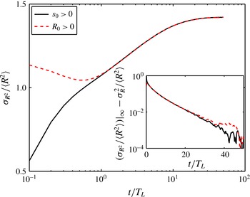
Time behaviour of the droplet surface normalized standard deviation $\unicode[STIX]{x1D70E}_{R^{2}}/\langle R^{2}\rangle$ in lin–log for two different initial conditions but the same model parameters $A$ and $\langle W\rangle$ . Red dashed line, initially delta function in $R>0$ and zero mean normal distribution for $s$ ; black solid line, initially zero sized droplets ( $R=0$ ) and constant positive $S>0$ . Inset: the same data but with the steady-state value subtracted and in a log–lin plot.

The system behaviour changes drastically when the drop size distribution becomes so wide that some droplets start to completely evaporate. Thereby, they lose their memory of their past history and they thus become independent of their initial condition. This is apparent in figure 10, where the time evolutions of two MC simulations with different initial conditions but the same parameters $A$ and $\langle W\rangle$ are compared. While the time evolutions depend on the initial conditions at short times and are thus very different, they converge towards each other and coincide at long times.

The time at which the diffusive short-time behaviour ends and a transition to the long-time behaviour starts is the time at which complete evaporation becomes significant. This evaporation time $T_{evap}$ can be estimated as the time where $2\unicode[STIX]{x1D70E}_{R^{2}}\sim \langle R^{2}\rangle$ . From (5.1b ), one obtains (in the limit of $T\gg \unicode[STIX]{x1D6E9}$ )

This time scale was already shown in figure 5 to mark the transition from the diffusive behaviour to the convergence to the steady state. If we want to observe the diffusive behaviour on time scales of the order of $t_{s}$ , the time until first evaporation has to satisfy $t_{evap}>t_{s}$ . For $\unicode[STIX]{x1D6E9}$ small, this leads to

It should be noted that a harmonic mean of $t_{s}$ and $\unicode[STIX]{x1D70F}_{s}$ appears; see (5.2). This is very close to the initial phenomenological reasoning $\unicode[STIX]{x1D70F}_{c}>\min (\unicode[STIX]{x1D70F}_{s},t_{0})$ that was used to distinguish between the two regimes found in the DNS (see § 2.2). Moreover, Paoli & Shariff (Reference Paoli and Shariff2009) could collapse the time dependence of their DNS results by normalizing time with the harmonic mean of $t_{0}$ and $\unicode[STIX]{x1D70F}_{s}$ . As a rule of thumb, it can be stated that the short-time behaviour containing no evaporated droplets is always present. However, when $\langle W\rangle$ is smaller than one, it is too short to be identified.

Figure 11.

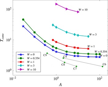
The exponential convergence time scale $T_{conv}$ as a function of the parameter $A$ and with the parameter $\langle W\rangle$ ranging from $0$ to $10$ . As in figure 7, the DNS values of the cases C7, C8 and C9 with $\langle W\rangle \sim 0$ and C4 and C6 with $\langle W\rangle \sim 0.354$ are superimposed.

5.2 Long-time behaviour

The long-time evolution of the system is independent of the initial conditions (see figure 10). It can be expected that the system will converge exponentially to the steady state with a rate given by the largest eigenvalue of the Fokker–Planck equation associated with the stochastic dynamics (3.3). This is confirmed in the inset of figure 10. The exponential convergence time $T_{conv}$ can be measured and is plotted in figure 11. The curves are very similar to the steady-state values of $\langle s\rangle _{E}$ , and the behaviour can be explained by the same arguments. The larger the parameter $A$ is, the stronger the bias due to the coupling term is, i.e. the waiting time to be evaporated shortens. For large $A$ , the convergence time seems to saturate to approximately $2.75t_{s}$ for $\langle W\rangle =0$ . At larger masses $\langle W\rangle$ , the convergence to the steady state is slower. Since the mean droplet size is larger (see figure 7), the time needed for droplets to completely evaporate increases. In DNS, the convergence to the steady state is faster than in the model. This was already visible from figure 5, albeit it can also be seen that the measurements are less certain and the fluctuations of the moments of $R$ are stronger. Nevertheless, the trends with respect to $A$ and $\langle W\rangle$ seem to be consistent with the behaviour obtained from the model.