



1. Introduction
Epidemic propagation, chemical reactions, opinion dynamics, flow control in the Internet, and even neural computations can all be modeled via punctuate interactions between interconnected agents [Reference Amblard and Deffuant1,Reference Baccelli, McDonald and Reynier2,Reference Gupta, Briat and Khammash11,Reference Pastor-Satorras, Castellano, Van Mieghem and Vespignani16,Reference Shriki, Alstott, Carver, Holroyd, Henson, Smith, Coppola, Bullmore and Plenz19]. The phenomena of interest in this context are idealized as network dynamics on a graph of agents which interact via point processes: edges between agents are the support of the interactions, with edge-specific point processes registering the times at which these interactions are exerted. Such point-process-based network dynamics constitute a very versatile class of models able to capture phenomena in natural sciences, engineering, social sciences, and economics. However, this versatility comes at the cost of tractability as the mathematical analysis of these dynamics is impossible except for the simplest network architectures. As a result, one has to resort to simplifying assumptions to go beyond numerical simulations.
Generic point-process-based networks are computationally intractable because their stochastic dynamics does not appear to belong to any known parametric class of point processes. Replica-mean-field (RMF) limits are precisely meant to circumvent this obstacle [Reference Baccelli and Taillefumier3]. The RMF limit of a given network is an extension of the network built in such a way that the interaction point processes are parametric, e.g. Poisson. This extended network is made of infinitely many replicas of the initial network, all with the same basic structure, but with randomized interactions across replicas. The interest in RMF limits stems from the fact that they offer a tractable version of the original dynamics that retain some of its most important features. The fact that Poisson point processes arise in the RMF version of a network is called the ‘Poisson hypothesis’. Thus formulated, the Poisson hypothesis originates from communication network theory [Reference Kleinrock13] and is distinct from replica approaches developed in statistical physics [Reference Castellani and Cavagna6].
Although intuitively clear and despite its usefulness, the Poisson hypothesis is often only conjectured and/or numerically validated. The purpose of this work is to rigorously establish the Poisson hypothesis for the RMF limits of a broad class of point-process-based network dynamics in discrete time introduced here. This class, which will be referred to as fragmentation-interaction-aggregation processes (FIAPs), includes important classes of queueing networks as special cases, as well as discrete-time Galves–Löcherbach (GL) neural networks.
Galves–Löcherbach networks can be viewed as coupled Hawkes processes with spike-triggered memory resets. Because of these memory resets, it can be shown that the dynamics of finite-sized GL networks is Markovian [Reference Robert and Touboul17]. The RMF limit of the GL case was studied from a computational standpoint in [Reference Baccelli and Taillefumier3] but in continuous time. In the next subsection we use results established in [Reference Baccelli and Taillefumier3] to illustrate how the Poisson hypothesis yields tractable mean-field equations for the stationary dynamics of these RMF limits. This is done for the simplest example of GL networks, called the ‘counting-neuron’ model.
1.1. Illustration from the study of spiking neural networks
The counting-neuron model consists of a fully connected network of K exchangeable neurons with homogeneous synaptic weights
 $\mu$
. For each neuron i,
 $1 \leq i \leq K$
, the continuously time-indexed stochastic intensity
 $\lambda_i$
increases by
 $\mu>0$
upon reception of a spike, and resets upon spiking to its base rate
 $b>0$
. Thus, its stochastic intensity is
 $\lambda_i(t)=b+\mu C_i(t)$
, where
 $C_i(t)$
is the number of spikes received at time t since the last reset. It can be shown that the network state
 $\lbrace C_1(t), \dots , C_K(t) \rbrace$
has a well-defined stationary distribution. Despite the simplicity of the model, analytic characterizations of the stationary state, including the stationary spiking rate, are hindered by the fact that the law of the point process of spike receptions is not known.
To circumvent this hindrance, the RMF setting proposes to compute stationary spiking rates in infinite networks that are closely related to the original finite-sized networks. Informally, the counting-model RMF is constructed as follows: for a K-neuron counting model and for an integer
 $M>0$
, the M-replica model consists of M replicas, each comprising K counting neurons. Upon spiking, a neuron i in replica m, indexed by (m,i), delivers spikes with synaptic weight
 $\mu$
to the
 $K-1$
neurons
 $(v_j,j)$
,
 $j\neq i$
, where the replica destination
 $v_j$
is chosen uniformly at random for all j. RMF networks are defined in the limit of an infinite number of replicas, namely infinite M but fixed and finite K. The Poisson hypothesis then states that the dynamics of replicas become asymptotically independent in the limit
 $M \to \infty$
, and that each neuron receives spikes from independent Poisson point processes. It is shown in [Reference Baccelli and Taillefumier3] that as a consequence of this Poisson property, the stationary state is characterized by a single ordinary differential equation (ODE) bearing on G, the probability-generating function (PGF) of a neuron count C:
 \begin{equation} \beta - \mu z G'(z) + \big(\beta (K - 1)(z - 1) - b \big)G(z) = 0 .\end{equation}
The simplifications warranted by the Poisson hypothesis in the above ODE characterization come at the cost of introducing the spiking rate
 $\beta$
as an unknown parameter in (1). As the ODE (1) is otherwise analytically tractable, characterizing the RMF stationary state amounts to specifying the unknown firing rate
 $\beta$
. Then, the challenge of the RMF approach consists in specifying the unknown firing rate via purely analytical considerations about a parametric system of ODEs. It turns out that requiring that the solution of (1) be analytic, as any PGF shall be, is generally enough to exhibit self-consistent relations about the stationary rates. For instance, the RMF stationary spiking rate
 $\beta$
of the RMF counting model is shown to be determined as the unique solution of
 \begin{equation*}\beta = \frac{\mu c^a \mathrm{e}^{-c}}{\gamma (a,c)}\end{equation*}
with
 $a = \frac{1}{\mu}[(K-1)\beta+b]$
and
 $c = \frac{1}{\mu}[(K-1)\beta]$
, where
 $\gamma$
denotes the lower incomplete Euler gamma function.
We have shown that the above approach generalizes to networks with continuous state space, heterogeneous network structures [Reference Baccelli and Taillefumier3], and including pairwise correlations [Reference Baccelli and Taillefumier4]. In all cases, the Poisson hypothesis is the cornerstone of a computational treatment. As a key step toward establishing the Poisson hypothesis for continuous-time network dynamics, the goal of this work is to prove it for a broad class of discrete-time dynamics, which we refer to as fragmentation-interaction-aggregation processes.
1.2. Fragmentation-interaction-aggregation processes
In FIAPs, agents are graph nodes endowed with a state that evolves over time. The nodes are coupled via point processes which model punctuate interactions. Specifically, each node’s state evolves in response to its input point process, and generates an output point process in a state-dependent manner. In all generality, the transformation of input into output point processes can be viewed as a random map. In FIAPs, this map is defined through the following dynamics: (i) The fragmentation process is triggered by local activation events taking place on each node that occur with a probability that depends on the state of the node. (ii) Each fragmentation event in turn triggers interactions between the nodes by creating input events in the neighboring nodes. (iii) Finally, the aggregation process consists in the integration of the input point processes to the states of each node.
Thus broadly defined, FIAPs offer a simple, albeit general, framework to analyze the phenomena alluded to above. The precise definition of a FIAP is given as follows:
Definition 1. An instance of the class
 $\mathcal{C}$
of discrete fragmentation-interaction-aggregation processes is determined by:
-
an integer K representing the number of nodes;
-
a collection of initial conditions for the integer-valued state variables at step zero, which we denote by
 $\{X_{i}\}$
, where
$i \in \{1,\ldots,K\}$
;
-
a collection of fragmentation random variables
$\{U_{i}\}$
, which are independent and identically distributed (i.i.d.) uniform in [0, 1] and independent of
$\{X_{i}\}$
, where
$i \in \{1,\ldots,K\}$
; -
a collection of fragmentation functions
$\{g_{1,i} \colon \mathbb{N} \rightarrow \mathbb{N}\}_{i \in \{1,\ldots,K\}}$
and
$\{g_{2,i} \colon \mathbb{N} \rightarrow \mathbb{N}\}_{i \in \{1,\ldots,K\}}$
; -
a collection of bounded interaction functions
$\{h_{i,j} \colon \mathbb{N} \rightarrow \mathbb{N}\}_{i,j \in \{1,\ldots,K\}}$
; -
a collection of activation probabilities
$\{\sigma_i(0), \sigma_i(1),\ldots\}_{i\in \{1,\ldots,K\}}$
verifying the conditions
$\sigma_i(0)=0$
and
$0<\sigma_i(1)\le \sigma_i(2)\le \cdots\le 1$
for all i.








The associated dynamics take as input the initial integer-valued state variables
 $\{X_{i}\}$
and define the state variables at the next step as
 \begin{equation}Y_{i}=g_{1,i}(X_{i})\textbf{1}_{\{U_{i}<\sigma_i(X_{i})\}}+g_{2,i}(X_{i})\textbf{1}_{\{U_{i}>\sigma_i(X_{i})\}}+A_{i}, \qquad \text{for all} \ i=1,\ldots,K,\end{equation}
with arrival processes
 $A_{i}=\sum_{j \neq i} h_{i,j}(X_{j})\textbf{1}_{\{U_{j}<\sigma_j(X_{j})\}}$
, for all
 $i=1,\ldots,K$
.
The interpretation is that node i activates with probability
 $\sigma_i(k)$
if its state
 $X_i$
is equal to k. The state of this node is fragmented to
 $g_{1,i}(k)$
upon activation and to
 $g_{2,i}(k)$
otherwise. This activation triggers an input of
 $h_{j,i}(k)$
units to node j. Hence, the interaction functions encode the structure of the graph. The variable
 $A_i$
gives the total number of arrivals to node i. This variable is aggregated to the state of the node as seen in (2). Note that considering
 $\sigma_i(0)=0$
for all i ensures that state variables in state 0 cannot be fragmented.
The FIAP class
 $\mathcal{C}$
encompasses many network dynamics relevant to queueing theory and mathematical biology. For example, taking
 $g_{1,i}(k)=k-1$
,
 $g_{2,i}(k)=k$
, and
 $h_{i,j}(k)=\textbf{1}_{\{i=j+1 \mod K\}}$
, we recover an instance of Gordon–Newell queueing networks [Reference Kleinrock12]. Taking
 $g_{1,i}(k)=0$
,
 $g_{2,i}(k)=k$
, and
 $h_{i,j}(k)=\mu_{i,j}\in \mathbb{N}$
defines a discrete instance of GL dynamics for the neural networks introduced above. Taking
 $g_{1,i}(k)=\lfloor \frac k 2 \rfloor$
and
 $g_{2,i}(k)=k+1$
corresponds to aggregation-fragmentation processes modeling, e.g., TCP communication networks [Reference Baccelli, McDonald and Reynier2]. The class
 $\mathcal{C}$
also includes certain discrete-time Hawkes processes. Namely, if, for each coordinate of a Hawkes vector process, we define its state as the sum over time of all its variations, then all discrete Hawkes processes that are Markov with respect to their so-defined state are in
 $\mathcal{C}$
. Thus, the results of the present paper have potential computational implications in a wide set of application domains beyond the neural network setting used above to illustrate them.
The present paper is focused on discrete-time versions of this type of dynamics as in, e.g., [Reference Cessac7,Reference Seol18]; note that continuous instances were also considered in the literature, such as in [Reference Delattre, Fournier and Hoffmann8,Reference Masi, Galves, Löcherbach and Presutti15].
1.3. Replica models for fragmentation-interaction-aggregation networks
Finite RMF models are defined as a coupling of replicas of the network of interest by randomized routeing decisions. For a FIAP, the state of its M-replica model is thus specified by a collection of state variables
 $X^{M}_{m,i}$
, where m is the index of the replica and i corresponds to the index of the node in the original network. Instead of interacting with nodes within the same replica, an activated node i in replica m interacts with a downstream node j from a replica n chosen uniformly at random and independently. This randomization preserves essential features of the original dynamics, such as the magnitude of interactions between nodes, but degrades the dependence structure between nodes. Indeed, over a finite period of time, the probability for a particular node to receive an activation from another given node scales as
 $1/M$
. Thus, as the number of replicas increases, interactions between distinct replicas become ever scarcer, intuitively leading to replica independence when
 $M \to \infty$
. This asymptotic independence is the root of RMF computational tractability.
Here is the precise definition of the finite-replica version of a FIAP:
Definition 2. For any process in
 $\mathcal{C}$
, the associated M-replica dynamics is entirely specified by:
-
a collection of initial conditions for the integer-valued state variables at step zero, which we denote by
$\{X^{M}_{n,i}\}$
, where
$n \in \{1,\ldots,M\}$
and
$i \in \{1,\ldots,K\}$
, such that for all
$M, n, i$
,
$X^M_{n,i}=X_i$
; -
a collection of fragmentation random variables
$\{U_{n,i}\}$
, which are i.i.d. uniform in [0, 1] and independent of
$\{X^{M}_{n,i}\}$
, where
$n \in \{1,\ldots,M\}$
and
$i \in \{1,\ldots,K\}$
; -
a collection of i.i.d. routeing random variables
$\{R^M_{m,j,i}\}$
independent of
$\{X^{M}_{n,i}\}$
and
$\{U_{n,i}\}$
, uniformly distributed on
$\{1,\ldots,M\}{\setminus}\{m\}$
for all
$i,j \in \{1,\ldots,K\}$
and
$m \in \{1,\ldots,M\}$
. In other words, if
$R^M_{m,j,i}=n$
, then an eventual activation of node j in replica m at step 0 induces an arrival of size
$h_{i,j}(X^M_{m,j})$
in node i of replica n, and n is chosen uniformly among replicas and independently of the state variables. Note that these variables are defined regardless of the fact that an activation actually occurs. Also note that for
$i'\ne i$
, the activation in question will induce an arrival in node i’ of replica n’, with n’ sampled in the same way but independently of n.






Then, the integer-valued state variables at step one, denoted by
 $\{Y^{M}_{n,i}\}$
, are given by the M-RMF equations
 $Y^{M}_{n,i}=g_{1,i}(X^{M}_{n,i})\textbf{1}_{\{U_{n,i}<\sigma_i(X^{M}_{n,i})\}}+g_{2,i}(X^{M}_{n,i})\textbf{1}_{\{U_{n,i}>\sigma_i(X^{M}_{n,i})\}}+A^M_{n,i}$
, where
 $g_{1,i}$
,
 $g_{2,i}$
denote fragmentation functions,
 $\sigma_i$
denotes activation probabilities, and where
 $A^M_{n,i}=\sum_{m \neq n}\sum_{j \neq i} h_{i,j}(X^M_{m,j})\textbf{1}_{\{U_{m,j}<\sigma_i(X^{M}_{m,j})\}}\textbf{1}_{\{R^M_{m,j,i}=n\}}$
is the number of arrivals to node i of replica n via the interaction functions
 $h_{i,j}$
.
RMF models are only expected to become tractable when individual replicas become independent. This happens in the limit of an infinite number of replicas, i.e. in the so-called RMF limit [Reference Baccelli and Taillefumier3]. In this RMF limit, asymptotic independence between replicas follows from the more specific Poisson hypothesis. The Poisson hypothesis states that spiking deliveries to distinct replicas shall be asymptotically distributed as independent Poisson (or compound) point processes. Such a hypothesis, which has been numerically validated for certain RMF networks, has been conjectured for linear Galves–Löcherbach dynamics in [Reference Baccelli and Taillefumier3]. Proving the validity of the Poisson hypothesis for the RMF limits of the much more general FIAPs is the purpose of the present work.
1.4. Methodology for proving the Poisson hypothesis
Classical mean-field approximations of a given network are obtained by considering the limit of the original network when a certain characteristic of the network, typically the number of nodes, goes to infinity. When the dynamics of the nodes are synchronous, one gets a discrete-time dynamical system. The term ‘mean field’ comes from the fact that in such network limits, the effects that individual nodes have on one another are approximated by a single averaged effect, typically an empirical mean. In the limit, this empirical mean usually converges to an expectation term through a propagation of chaos result [Reference Sznitman20] which leads to analytical tractability. In replica mean fields, there is no such empirical mean over the nodes of the network; the mean-field simplification comes from the random routeing operations between replicas. The input point process in the M-replica model consists in a superposition of M rare point processes, which informally explains why Poisson (or compound Poisson) processes arise at the limit. For classical mean fields, different techniques have been developed to prove the existence of and convergence to the mean-field limit. Standard techniques include the use of the theory of nonlinear Markov processes [Reference Vladimirov, Pirogov, Rybko and Shlosman21] and stochastic approximation algorithms [Reference Benaim and Le Boudec5] for continuous-time dynamics, and induction techniques which assume the existence of limits at time zero and extend the result by induction [Reference Le Boudec, McDonald and Mundinger14] for dynamics in discrete time. Refinements to the latter approach can be made in order to obtain explicit rates of convergence [Reference Gast, Latella and Massink10]. The approach developed for the RMF case belongs in spirit to the third class of techniques. We suppose that the property of asymptotic independence (see Definition 3) holds for the state variables at time zero. We then prove that this property is preserved by the dynamics of the M-replica model and thus holds by induction for any finite time. Thus, we focus hereafter on the one-step transition of the model from time 0 to time 1. We show that this asymptotic independence hypothesis implies both convergence in distribution and an ergodic type property that we call the triangular law of large numbers. We apply this law of large numbers to the input process to a single node to show that Poisson (or compound Poisson) processes indeed appear in the replica-mean-field limit. We stress that this proof is by induction. The fact that the main difficulty consists in proving the induction step should not hide the fact that the result relies in a crucial way on the assumption that at step 0, the initial state variables satisfy the asymptotic independence property. Whether the result can be extended to more general initial conditions is an open question at this stage.
1.5. Structure of the paper
For the sake of clarity in exposition, we start with the proof of the Poisson hypothesis for the special case of neural networks, before extending it to general FIAPs. More precisely, we first consider the symmetric neural network case, which is a fully symmetric GL model [Reference Galves and Löcherbach9] in discrete time. We introduce the model in Section 2 and prove the Poisson hypothesis in Section 3. We then extend the proof to the class of FIAPs defined above. We first consider the symmetric case in Section 4, and then the general case in Section 5. Finally, some extensions are discussed in Section 6.
2. The symmetric Galves–Löcherbach model
2.1. The symmetric RMF network model
We consider a network of K spiking neurons. We suppose that the behavior of each neuron is determined by a random variable representing the membrane potential of the neuron. Each neuron spikes at a rate depending on its state variable. Let
 $X=\{X_{i}\}$
be the integer-valued state variables at step 0, where
 $i \in \{1,\ldots,K\}$
. Let
 $Y=\{Y_{i}\}$
be the integer-valued state variables at time 1. The system continues to evolve in discrete time with all corresponding state variables defined by induction.
Let
 $\sigma \colon \mathbb{N} \rightarrow [0,1]$
be the spiking probabilities of the neurons. Namely,
 $\sigma(k)$
is the probability that a neuron in state k spikes. We consider that
 $\sigma(0)=0$
, accounting for the fact that a neuron in state 0 never spikes. We also consider that
 $\sigma(1)>0$
and that
 $\sigma$
is nondecreasing. Let
 $\{U_{i}\}$
be uniformly distributed i.i.d. random variables independent of
 $\{X_{i}\}$
. We then write, for the evolution equation for the state of the system,
 $Y_{i}=\textbf{1}_{\{U_{i}>\sigma(X_{i})\}} X_{i}+A_{i}$
, where
 $A_{i}=\sum_{j \neq i} \textbf{1}_{\{U_{j}<\sigma(X_{j})\}}$
is the number of arrivals to neuron i.
Here, the fragmentation is complete if
 $U_{i}<\sigma(X_{i})$
, namely if there is a spike, in which case the state variable is reset (jumps to 0). Otherwise there is no fragmentation at all and the state variable is left unchanged. In both cases, the arrivals
 $A_i$
are aggregated to the state.
The RMF model described below is a discrete-time version of the model introduced in [Reference Baccelli and Taillefumier3]. Namely, we consider a collection of M identically distributed replicas of the initial set of K neurons. Let
 $X=\{X^{M}_{n,i}\}$
be the integer-valued state variables at step 0, where
 $n \in \{1,\ldots,M\}$
,
 $i \in \{1,\ldots,K\}$
. Let
 $Y=\{Y^{M}_{n,i}\}$
be the integer-valued state variables at time 1. Let
 $U=\{U_{n,i}\}$
be uniformly i.i.d. random variables in [0, 1] independent of
 $\{X^{M}_{n,i}\}$
. Let
 $R=\{R^M_{m,i,j}\}$
be i.i.d. routeing random variables independent of
 $\{X^{M}_{n,i}\}$
and
 $\{U_{n,i}\}$
, uniformly distributed on
 $\{1,\ldots,M\}{\setminus}\{m\}$
for all
 $i,j \in \{1,\ldots,K\}$
and
 $m \in \{1,\ldots,M\}$
. The replica model has the evolution equation
 \begin{equation}Y^{M}_{n,i}=\textbf{1}_{\left\{U_{n,i}>\sigma\left(X^{M}_{n,i}\right)\right\}} X^{M}_{n,i}+A^M_{n,i},\end{equation}
where
 \begin{equation}A^M_{n,i}=\sum_{m \neq n}\sum_{j \neq i} \textbf{1}_{\left\{U_{m,j}<\sigma\left(X^{M}_{m,j}\right)\right\}}\textbf{1}_{\left\{R^M_{m,j,i}=n\right\}}\end{equation}
is the number of arrivals to neuron i of replica n.
2.2. Pairwise asymptotic independence and consequences
Our goal is to show the propagation of chaos and the Poisson hypothesis in this system. In other words, we want to show that the arrivals to two distinct replicas are asymptotically independent, and the number of arrivals to one replica is asymptotically Poisson distributed. We begin by considering the fully exchangeable case with equal weights, but we will consider the general case later. In order to do so, we choose to characterize the propagation of chaos through the following properties.
Definition 3. Given
 $M \in \mathbb{N}$
, given an array of integer-valued random variables
 $Z=\{Z^{M}_{n,i}\}_{1 \leq n \leq M, 1 \leq i \leq K}$
such that, for all fixed M, the random variables
 $Z^M_{n,i}$
are exchangeable in n and i, we say that the variables
 $Z^M_{n,i}$
are pairwise asymptotically independent, which we will denote PAI(Z), if there exists an integer-valued random variable
 $\tilde{Z}$
such that, for all
 $(n,i) \neq (m,j)$
, for all
 $u,v \in [0,1]$
,
 $\lim_{N \rightarrow \infty}\mathbb{E}\big[u^{Z^N_{n,i}}v^{Z^N_{m,j}}\big] =\mathbb{E}\big[u^{\tilde{Z}}\big]\mathbb{E}\big[v^{\tilde{Z}}\big]$
.
Definition 4. Given
 $M \in \mathbb{N}$
, given an array of integer-valued random variables
 $Z=\{Z^{M}_{n}\}_{n \in \{1,\ldots,M\}}$
such that, for all fixed M, the random variables
 $Z^M_{n}$
are exchangeable in n, we say that Z satisfies the triangular law of large numbers, denoted by TLLN(Z), if there exists an integer-valued random variable
 $\tilde{Z}$
such that, for all functions
 $f \colon \mathbb{N}\rightarrow \mathbb{R}$
with compact support, we have the following limit in
 $L^2$
:
 $\lim_{N\rightarrow\infty}\frac{1}{N}\sum_{n=1}^N f(Z_{n}^N)=\mathbb{E}[f(\tilde{Z})]$
.
We have a few remarks about these definitions. First, note that if an array of random variables Z satisfies PAI(Z) then, for all n and i,
 $Z^M_{n,i}$
converges in distribution to
 $\tilde{Z}$
as
 $M \rightarrow \infty$
. This can be seen by taking
 $v=1$
in the definition. By considering the case where
 $Z^M_{n}=Z^1_1$
for all n and M, we see that the convergence in distribution of
 $Z^M_{n}$
does not imply TLLN(Z). However, we show below that for all arrays of random variables
 $Z=\{Z^{M}_{n,i}\}_{n \in \{1,\ldots,M\}, i \in \{1,\ldots,K\}}$
satisfying PAI(Z), for all i,
 $Z_i=\{Z^{M}_{n,i}\}_{n \in \{1,\ldots,M\}}$
satisfies
 $TLLN(Z_i)$
. In other words, pairwise asymptotic independence of an array of random variables implies that these random variables satisfy the triangular law of large numbers. Finally, note that an array of integer-valued random variables Z satisfies PAI(Z) if and only if the random variables are asymptotically independent in the sense that, for all
 $(n,i) \neq (m,j)$
,
 $\mathbb{P}\big(Z^M_{n,i} \in B_1, Z^M_{m,j} \in B_2\big) \rightarrow \mathbb{P}(\tilde{Z} \in B_1)\mathbb{P}(\tilde{Z} \in B_1)$
when
 $M \rightarrow \infty$
for
 $B_1, B_2 \in \mathcal{B}(\mathbb{R})$
.
The following characterization of
 $L^2$
convergence will be used throughout this paper.
Lemma 1. Let
 $(X_n)$
be random variables with finite second moments. Then there exists a constant c such that
 $X_n \rightarrow c$
in
 $L^2$
when
 $n \rightarrow \infty $
if and only if
-
(i)
$\mathbb{E}[X_n] \rightarrow c$
when
$n \rightarrow \infty$
; -
(ii)
$\text{var}(X_n) \rightarrow 0$
when
$n \rightarrow \infty$
.


This follows directly from the definition of
 $L^2$
convergence.
The following lemma describes the relation between pairwise asymptotic independence and the triangular law of large numbers.
Lemma 2. Let
 $M \in \mathbb{N}$
, and let
 $Z=\big\{Z^{M}_{n,i}\big\}_{n \in \{1,\ldots,M\}, i \in \{1,\ldots,K\}}$
be an array of integer-valued random variables verifying PAI(Z). Then, for all i,
 $Z_i=\big\{Z^{M}_{n,i}\big\}_{n \in \{1,\ldots,M\}}$
satisfies
 $\textrm{TLLN}(Z_i)$
.
Proof. Let
 $f \colon \mathbb{N} \rightarrow \mathbb{R}$
be a function with compact support. We use Lemma 1. We fix
 $i \in \{1,\ldots,K\}$
, which we omit in the rest of the proof. We have
 \begin{align*}\text{var}\left(\frac{1}{M}\sum_{n=1}^M f\big(Z^M_n\big)\right)& = \frac{1}{M^2}\left(\sum_{n=1}^M \text{var}\left(f\big(Z^M_n\big)\right)+\sum_{p \neq q}\text{cov}\big[f\big(Z^M_p\big),f\big(Z^M_q\big)\big]\right) \\& = \frac{1}{M}\text{var}\left(f\big(Z^M_1\big)\right)+\frac{M(M-1)}{M^2}\text{cov}\big[f\big(Z^M_1\big),f\big(Z^M_2\big)\big],\end{align*}
the last equality holding by exchangeability between replicas. Both terms on the right-hand side go to 0 when
 $M \rightarrow \infty$
. For the first term, this follows from the boundedness of f. For the second, we first show the result for indicator functions. Let
 $B \in \mathcal{B}(\mathbb{R})$
and let f be defined by
 $f(n)=\textbf{1}_{\{n\in B\}}$
. Then we have
 $\text{cov}\big[f\big(Z^M_1\big),f\big(Z^M_2\big)\big]=\mathbb{P}\big(Z^M_1\in B,Z^M_2\in B\big)-\mathbb{P}\big(Z^M_1\in B\big)\mathbb{P}\big(Z^M_2\in B\big)$
, which goes to 0 when
 $M \rightarrow \infty$
by PAI(Z). This immediately extends to functions with compact support since they only take a finite number of values. Moreover, for all such functions,
 $\mathbb{E}\big[\frac{1}{M}\sum_{n=1}^M f(Z^M_n)\big] \rightarrow \mathbb{E}[f(\tilde{Z})]$
when
 $M \rightarrow \infty$
as a direct consequence of the fact that, for integer-valued random variables, convergence in distribution of
 $Z^M$
to
 $\tilde{Z}$
is equivalent to the convergence
 $\mathbb{P}(Z^M=k) \rightarrow \mathbb{P}(\tilde{Z}=k)$
for all
 $k \in \mathbb{N}$
. This concludes the proof.
For our subsequent needs, we also establish the following result: we show that pairwise asymptotic independence implies a property that is slightly more general than the triangular law of large numbers, where we allow the function f to depend on an array of i.i.d. random variables
 $U=\{U_{n,i}\}_{n \in \{1,\ldots,M\}, i \in \{1,\ldots,K\}}$
, independent of the rest of the dynamics.
Lemma 3. Let
 $M \in \mathbb{N}$
, and let
 $Z=\big\{Z^{M}_{n,i}\big\}_{n \in \{1,\ldots,M\}, i \in \{1,\ldots,K\}}$
be an array of integer-valued random variables satisfying PAI(Z). Then, for all bounded functions
 $f \colon \mathbb{N}\times [0,1] \rightarrow \mathbb{R}$
with compact support, for all i.i.d. sequences of random variables
 $U=\{U_{n,i}\}_{n \in \{1,\ldots,M\}, i \in \{1,\ldots,K\}}$
independent of Z, there exists
 $\tilde{U}$
independent from
 $\tilde{Z}$
and Z such that, for all
 $i \in \{1,\ldots,K\}$
, we have the following limit in
 $L^2$
:
 \begin{equation*}\lim_{M\rightarrow\infty}\frac{1}{M}\sum_{n=1}^M f\big(Z_{n,i}^M, U_{n,i}\big)=\mathbb{E}[f(\tilde{Z},\tilde{U})].\end{equation*}
Note that compared to Definition 4, we consider that the functions are bounded, a condition that was automatically fulfilled for functions with compact support on
 $\mathbb{N}$
.
Proof. We proceed as in the last lemma, conditioning on the
 $U_{n,i}$
when necessary. Let
 $M \in \mathbb{N}$
, let
 $i \in \{1,\ldots,K\}$
. We will omit this index in the rest of the proof. By exchangeability between replicas, defining
 $\tilde{U}=U_1$
, we have
 $\mathbb{E}\left[\frac{1}{M}\sum_{n=1}^M f\big(Z^M_{n}, U_n\big)\right] =\mathbb{E}\big[f\big(Z^M_1,U_1\big)\big]=\mathbb{E}\big[f\big(Z^M_1,\tilde{U}\big)\big]$
. Since
 $Z^M_1$
converges in distribution to
 $\tilde{Z}$
when
 $M \rightarrow \infty$
, and since
 $Z^M_1$
is integer valued and f is bounded, for all
 $u \in [0,1]$
,
 $\mathbb{E}\big[f\big(Z^M_1,u\big)\big] \rightarrow \mathbb{E}[f(\tilde{Z},u)]$
when
 $ M \rightarrow \infty$
. Therefore, since
 $\tilde{U}$
is independent of Z and
 $\tilde{Z}$
,
 $\mathbb{E}\big[f\big(Z^M_1,\tilde{U}\big)\big] \rightarrow \mathbb{E}[f(\tilde{Z},\tilde{U})]$
when
 $M \rightarrow \infty$
almost surely. Finally,
 \begin{equation*}\mathbb{E}\left[\frac{1}{M}\sum_{n=1}^M f\big(Z^M_{n},U_n\big)\right] \rightarrow \mathbb{E}\left[f(\tilde{Z},\tilde{U})\right]\end{equation*}
when
 $M \rightarrow \infty$
. Moreover,
 \begin{align*}& \text{var}\left(\frac{1}{M}\sum_{n=1}^M f\big(Z^M_{n}, U_n\big)\right) \\& \quad = \frac{1}{M^2}\sum_{n=1}^M \text{var}\left(f\big(Z^M_n,U_n\big)\right)+\frac{1}{M^2}\sum_{n\neq n'}\text{cov}\left[f\big(Z^M_n,U_n\big),f\big(Z^M_{n'},U_{n'}\big)\right]\\& \quad = \frac{1}{M}\text{var}\left(f\big(Z^M_1,U_1\big)\right)+\frac{M(M-1)}{M^2}\text{cov}\left[f\big(Z^M_1,U_1\big),f\big(Z^M_2,U_2\big)\right],\end{align*}
the last equality stemming from exchangeability between replicas. When
 $M \rightarrow \infty$
, the first term goes to 0 because f is bounded. For the second term, since the
 $\{Z^M_n\}$
and the
 $\{U_n\}$
are independent and the
 $\{U_n\}$
are i.i.d., we can proceed as above. Namely, let
 $B, C \in \mathcal{B}(\mathbb{R})$
. Let f be defined by
 $f(n,t)=\textbf{1}_{\{n \in B\}}\textbf{1}_{\{t \in C\}}$
. Then we have
 \begin{align*}& \text{cov}\big[f\big(Z^M_1,U_1\big),f\big(Z^M_2,U_2\big)\big]\\[4pt] &\quad = \mathbb{P}\big(Z^M_1\in B,Z^M_2\in B, U_1 \in C, U_2 \in C\big)-\mathbb{P}\big(Z^M_1\in B, U_1 \in C\big)\mathbb{P}\big(Z^M_2\in B, U_2 \in C\big) \\[4pt] &\quad = \left(\mathbb{P}\big(Z^M_1\in B,Z^M_2\in B\big)-\mathbb{P}\big(Z^M_1\in B\big)\mathbb{P}\big(Z^M_2\in B\big)\right)\mathbb{P}(U_1 \in C)\mathbb{P}(U_2 \in C),\end{align*}
the last equality holding by independence between Z and
 $\{U_{n,i}\}_{n \in \{1,\ldots,M\}, i \in \{1,\ldots,K\}}$
. The right-hand term goes to 0 when
 $M \rightarrow \infty$
by PAI(Z). This generalizes to bounded functions with compact support, which concludes the proof.
2.3. Main result
Our goal is to show that if
 $X=\big\{X^{M}_{n,i}\big\}$
are asymptotically independent, then
 $Y=\big\{Y^{M}_{n,i}\big\}$
are as well. In other words, if we choose initial conditions that satisfy a certain property, this property will hold by induction at any finite discrete time.
Theorem 1. Let
 $M \in \mathbb{N}$
, and let
 $X=\{X^{M}_{n,i}\}_{n \in \{1,\ldots,M\}, i \in \{1,\ldots,K\}}$
be an array of integer-valued random variables (the ‘state variables’). Suppose that PAI(X) holds. Then PAI(Y) holds as well, where Y is defined by (3). Moreover, the arrivals to a given node
 $A^M_{n,i}$
converge in distribution to a Poisson random variable when
 $M \rightarrow \infty$
.
Note that the result depends on a choice of initial conditions verifying PAI(X), a typical example of which is i.i.d. initial conditions stable in law, in the sense that their law does not depend on M. The question of whether, given an arbitrary initial condition, the dynamics become pairwise asymptotically independent after some (finite or infinite) amount of time, is still open. Note also that this shows that we have convergence in distribution of the exchangeable variables
 $\big\{Y^M_n\big\}$
when
 $M \rightarrow \infty$
.
3. Proof of Theorem 1
In the following proof, since K is always finite and all the random variables considered are exchangeable, as above, we will sometimes omit the neuron index
 $i \in \{1,\ldots,K\}$
in order to simplify notation. Tilde superscripts will refer to objects in the infinite replica limit. Hat superscripts will refer to fragmentation processes.
3.1. Fragmentation
Lemma 4. Let
 $\hat{X}=\left\{\hat{X}^{M}_{n,i}=X^{M}_{n,i} \textbf{1}_{\left\{U_{n,i}>\sigma\left(X^{M}_{n,i}\right)\right\}}\right\}$
. Then PAI(X) implies
 $PAI(\hat{X})$
.
Proof. We have, for
 $u,v \in [0,1]$
,
 $\mathbb{E}\big[u^{\hat{X}^M_1}v^{\hat{X}^M_2}\big]=\sum_{k,l \in \mathbb{N}}\mathbb{P}\big(\hat{X}^M_1=k,\hat{X}^M_2=l\big)u^k v^l$
. For
 $k,l >0$
, we have
 $\mathbb{P}\big(\hat{X}^M_1=k,\hat{X}^M_2=l\big)=\mathbb{P}\big(X^M_1=k,X^M_2=l\big)(1-\sigma(k))(1-\sigma(l))$
. Similarly,
 $\mathbb{P}\big(\hat{X}^M_1=k,\hat{X}^M_2=0\big) = \sum_{l\in \mathbb{N}}\mathbb{P}\big(X^M_1=k,X^M_2=l\big)(1-\sigma(k))\sigma(l)$
for all
 $k>0$
, and
 $\mathbb{P}\big(\hat{X}^M_1=0,\hat{X}^M_2=0\big) = \sum_{k,l\in \mathbb{N}}\mathbb{P}\big(X^M_1=k,X^M_2=l\big)\sigma(k)\sigma(l)$
. Since PAI(X) holds, for all
 $k,l \in \mathbb{N}$
,
 $\mathbb{P}\big(X^M_1=k,X^M_2=l\big) \rightarrow \mathbb{P}(\tilde{X}=k)\mathbb{P}(\tilde{X}=l)$
when
 $M \rightarrow \infty$
. Since all the functions considered are bounded by 1, we have, for all
 $k,l \in \mathbb{N}$
,
 $\mathbb{P}\big(\hat{X}^M_1=k,\hat{X}^M_2=l\big) \rightarrow \mathbb{P}\big(\tilde{\hat{X}}=k\big)\mathbb{P}\big(\tilde{\hat{X}}=l\big)$
when
 $M \rightarrow \infty$
, where
 $\tilde{\hat{X}}=\tilde{X}\textbf{1}_{\left\{U>\sigma\left(\tilde{X}\right)\right\}}$
. This shows that
 $\mathbb{E}\big[u^{\hat{X}^M_1}v^{\hat{X}^M_2}\big] \rightarrow \mathbb{E}\big[u^{\tilde{\hat{X}}}\big]\mathbb{E}\big[v^{\tilde{\hat{X}}}\big]$
when
 $M \rightarrow \infty$
, which concludes the proof.
3.2. Asymptotic behavior of the arrivals processes
We now show that the number of arrivals
 $A^M_{n,i}$
defined in (4) is asymptotically Poisson as the number of replicas goes to infinity. This is precisely the Poisson hypothesis introduced in [Reference Kleinrock13].
Lemma 5. Supposing that PAI(X) holds. When
 $M \rightarrow \infty$
, we have the convergence in distribution
 $A^M_{n,i} \rightarrow \mathrm{Poi}((K-1)\theta)$
, where
 $\theta=\mathbb{E}[\sigma(\tilde{X})]$
.
Proof. Let
 $z\in [0,1]$
. Then
 \begin{equation*}\begin{split}\mathbb{E}\big[z^{A^M_{n,i}}\big]&=\mathbb{E}\left[z^{\sum_{m \neq n}\sum_{j \neq i} \textbf{1}_{\left\{U_{m,j}<\sigma\left(X^{M}_{m,j}\right)\right\}}\textbf{1}_{\left\{R^M_{m,j,i}=n\right\}}}\right]\\[4pt]&=\mathbb{E}\left[\prod_{m\neq n}\prod_{j \neq i}\mathbb{E}\left[z^{ \textbf{1}_{\left\{U_{m,j}<\sigma\left(X^{M}_{m,j}\right)\right\}}\textbf{1}_{\left\{R^M_{m,j,i}=n\right\}}} \, \Big| \, X^M_{m,j},U\right]\right] \\[4pt]&=\mathbb{E}\left[\prod_{m\neq n}\prod_{j \neq i}\left(\left(1-\frac{1}{M-1}\right)+\frac{1}{M-1}z^{\textbf{1}_{\left\{U_{m,j}<\sigma\left(X^{M}_{m,j}\right)\right\}}}\right)\right] \\[4pt]&=\mathbb{E}\left[\exp\left\{\sum_{m \neq n}\sum_{j \neq i}\log\left(1-\frac{1}{M-1}\left(1-z^{\textbf{1}_{\left\{U_{m,j}<\sigma\left(X^{M}_{m,j}\right)\right\}}}\right)\right)\right\}\right].\end{split}\end{equation*}
We now give upper and lower bounds for this expression. Since
 $\log(1-x)\leq -x$
for
 $x\leq 1$
, we have
 \begin{equation*}\mathbb{E}\big[z^{A^M_{n,i}}\big]\leq \mathbb{E}\left[\exp\left\{-\frac{1}{M-1}\sum_{m \neq n}\sum_{j \neq i}\left(1-z^{\textbf{1}_{\left\{U_{m,j}<\sigma\left(X^{M}_{m,j}\right)\right\}}}\right)\right\}\right].\end{equation*}
Using the generalized TLLN given in Lemma 3,
 \begin{equation*}\frac{1}{M-1}\sum_{m \neq n}\sum_{j \neq i}\left(1-z^{\textbf{1}_{\left\{U_{m,j}<\sigma\left(X^{M}_{m,j}\right)\right\}}}\right) \rightarrow (K-1)(1-\Phi(z))\end{equation*}
in
 $L^2$
when
 $M \rightarrow \infty$
, with
 $\Phi(z)=\mathbb{E}\big[z^{\textbf{1}_{U<\sigma(\tilde{X})}}\big]$
, where U is any
 $U_{m,j}$
. We have
 $\Phi(z)=z\int_0^1\mathbb{P}(\sigma(\tilde{X})>t)\mathop{}\!\mathrm{d} t+\big(1-\int_0^1\mathbb{P}(\sigma(\tilde{X})>t)\mathop{}\!\mathrm{d} t\big)=(z-1)\theta+1.$
Therefore, since
 $L^2$
convergence implies convergence in distribution and thus convergence of the Laplace transforms,
 \begin{equation*}\mathbb{E}\left[\exp\left\{-\frac{1}{M-1}\sum_{m \neq n}\sum_{j \neq i}\left(1-z^{\textbf{1}_{\left\{U_{m,j}<\sigma\left(X^{M}_{m,j}\right)\right\}}}\right)\right\}\right] \rightarrow \mathrm{e}^{-\theta(1-z)(K-1)}\end{equation*}
when
 $M \rightarrow \infty$
. Thus,
 \begin{equation}\limsup_{M\rightarrow \infty}\mathbb{E}\big[z^{A^M_{n,i}}\big] \leq \mathrm{e}^{-\theta(1-z)(K-1)}.\end{equation}
Similarly, since
 $\log(1-x)\geq -x-\frac{x^2}{2}$
for
 $x\leq 1$
, we have
 \begin{multline*}\mathbb{E}\big[z^{A^M_{n,i}}\big]\geq \mathbb{E}\left[\exp\left\{-\frac{1}{M-1}\sum_{m \neq n}\sum_{j \neq i}\left(1-z^{\textbf{1}_{\left\{U_{m,j}<\sigma\left(X^{M}_{m,j}\right)\right\}}}\right)\right\}\right. \\ \left.\exp\left\{-\frac{1}{2(M-1)^2}\sum_{m \neq n}\sum_{j \neq i}\left(1-z^{\textbf{1}_{\left\{U_{m,j}<\sigma\left(X^{M}_{m,j}\right)\right\}}}\right)^2\right\}\right].\end{multline*}
Using once again Lemma 3, as the second term goes to 0 when
 $M \rightarrow \infty$
, by the same reasoning as previously, we get
 \begin{equation}\liminf_{M\rightarrow \infty}\mathbb{E}\big[z^{A^M_{n,i}}\big] \geq \mathrm{e}^{-\theta(1-z)(K-1)}.\end{equation}
Combining (5) and (6), the result follows.
Now, we show that the arrivals to different replicas become pairwise asymptotically independent.
Lemma 6. For all
 $(n,i) \neq (m,j)$
,
 $A^M_{n,i}$
and
 $A^M_{m,j}$
are pairwise asymptotically independent.
Proof. We first show the result in the case
 $n \neq m$
and
 $i \neq j$
. Let
 $u,v \in [0,1]$
. Then
 \begin{align*}\mathbb{E}\big[u^{A^M_{n,i}}v^{A^M_{m,j}}\big] & = \mathbb{E}\left[u^{\sum_{n' \neq n, i' \neq i}\textbf{1}_{\left\{U_{n',i'}<\sigma\left(X^M_{n',i'}\right)\right\}}\textbf{1}_{\left\{R^M_{n',i',i}=n\right\}}}\right. \\& \quad \qquad \left. v^{\sum_{m' \neq m, j' \neq j}\textbf{1}_{\left\{U_{m',j'}<\sigma\left(X^M_{m',j'}\right)\right\}}\textbf{1}_{\left\{R^M_{m',j',j}=m\right\}}}\right] \\[4pt]& = \mathbb{E}\left[\prod_{n' \neq n, i' \neq i}u^{\textbf{1}_{\left\{U_{n',i'}<\sigma\left(X^M_{n',i'}\right)\right\}}\textbf{1}_{\left\{R^M_{n',i',i}=n\right\}}}\right.\\& \quad \qquad \left. \prod_{m' \neq m, j' \neq j}v^{\textbf{1}_{\left\{U_{m',j'}<\sigma\left(X^M_{m',j'}\right)\right\}}\textbf{1}_{\left\{R^M_{m',j',j}=m\right\}}}\right] \\[4pt]& = \mathbb{E}\left[\mathbb{E}\left[\prod_{n' \neq n, i' \neq i}u^{\textbf{1}_{\left\{U_{n',i'}<\sigma\left(X^M_{n',i'}\right)\right\}}\textbf{1}_{\left\{R^M_{n',i',i}=n\right\}}}\right.\right.\\[6pt]& \qquad \qquad \left.\left. \prod_{m' \neq m, j' \neq j}v^{\textbf{1}_{\left\{U_{m',j'}<\sigma\left(X^M_{m',j'}\right)\right\}}\textbf{1}_{\left\{R^M_{m',j',j}=m\right\}}} \, \Big| \, X^M, U\right]\right] \\[6pt]& = \mathbb{E}\left[\prod_{n' \neq n, i' \neq i}\left[\left(1-\frac{1}{M-1}\right)+\frac{1}{M-1}u^{\textbf{1}_{\left\{U_{n',i'}<\sigma\left(X^M_{n',i'}\right)\right\}}}\right]\right. \\[6pt]& \quad \qquad \left. \prod_{m' \neq m, j' \neq j}\left[\left(1-\frac{1}{M-1}\right)+\frac{1}{M-1}v^{\textbf{1}_{\left\{U_{m',j'}<\sigma\left(X^M_{m',j'}\right)\right\}}}\right]\right] \\[6pt]& = \mathbb{E}\left[\exp\left\{\sum_{n' \neq n, i' \neq i}\log\left(1-\frac{1}{M-1}\left(1-u^{\textbf{1}_{\left\{U_{n',i'}<\sigma\left(X^M_{n',i'}\right)\right\}}}\right)\right)\right\}\right.\\[6pt]& \quad \qquad \left. \exp\left\{\sum_{m' \neq m, j' \neq j}\log\left(1-\frac{1}{M-1}\left(1-v^{\textbf{1}_{\left\{U_{m',j'}<\sigma\left(X^M_{m',j'}\right)\right\}}}\right)\right)\right\}\right].\end{align*}
The fourth equality above comes from the independence between the routeing variables
 $R^M$
.
Just as in the proof of Lemma 5, we can give upper and lower bounds of the last expression on the right-hand side:
 \begin{multline*}\mathbb{E}\big[u^{A^M_{n,i}}v^{A^M_{m,j}}\big] \leq \mathbb{E}\left[\exp\left\{-\frac{1}{M-1}\sum_{n' \neq n, i' \neq i}\left(2-u^{\textbf{1}_{\left\{U_{n',i'}<\sigma\left(X^M_{n',i'}\right)\right\}}}-v^{\textbf{1}_{\left\{U_{n',i'}<\sigma\left(X^M_{n',i'}\right)\right\}}}\right)\right\}\right]\end{multline*}
and
 \begin{align*}\mathbb{E}\big[&u^{A^M_{n,i}}v^{A^M_{m,j}}\big] \geq \mathbb{E}\left[\exp\left\{-\frac{1}{M-1}\sum_{n' \neq n, i' \neq i}\left(2-u^{\textbf{1}_{\left\{U_{n',i'}<\sigma\left(X^M_{n',i'}\right)\right\}}}-v^{\textbf{1}_{\left\{U_{n',i'}<\sigma\left(X^M_{n',i'}\right)\right\}}}\right)\right\} \right. \\[4pt]& \qquad\qquad \left. \exp\left\{-\frac{1}{2(M-1)^2}\sum_{m \neq n}\sum_{j \neq i}\left(2-u^{\textbf{1}_{\left\{U_{n',i'}<\sigma\left(X^M_{n',i'}\right)\right\}}}-v^{\textbf{1}_{\left\{U_{n',i'}<\sigma\left(X^M_{n',i'}\right)\right\}}}\right)^2\right\}\right]. \end{align*}
The last expression on the right-hand side goes to
 $\mathrm{e}^{(1-u+1-v)(K-1)\theta}$
when
 $M \rightarrow \infty$
in both cases, as previously. The result follows from these two bounds as in the proof of Lemma 5.
The case where
 $n=m$
, i.e. when we consider the arrivals to two different neurons in the same replica, is done in the same way since the routeing variables are independent of the neurons chosen. The case where
 $i=j$
, i.e. when we consider the arrivals to the same neuron in two different replicas, is treated in the same way, with the extra step of isolating the terms that are not independent of each other.
3.3. Propagation of pairwise asymptotic independence
Our goal is now to combine the previous results to show that PAI(Y) holds, assuming PAI(X). We have, for all
 $i \in \{1,\ldots,K\}$
and all
 $n \in \{1,\ldots,M\}$
,
 $Y^M_{n,i}=\hat{X}^M_{n,i}+A^M_{n,i}$
. We call
 $\tilde{A}$
the limit in distribution of
 $A^M_{n,i}$
(it is Poisson distributed by the previous lemma). It is clear that by exchangeability between replicas, we only require the following lemma.
Lemma 7. For
 $i,j \in \{1,\ldots,K\}$
,
 \begin{equation}\mathbb{E}\big[u^{Y^M_{1,i}},v^{Y^M_{2,j}}\big] \rightarrow \mathbb{E}\big[u^{\tilde{Y}}\big]\mathbb{E}\big[v^{\tilde{Y}}\big]\end{equation}
when
 $M \rightarrow \infty$
, where
 $\tilde{Y}=\tilde{\hat{X}}+\tilde{A}$
.
Proof. Let
 $u,v \in [0,1]$
. Then, given
 $i,j \in [0,K]$
, with
 $i \neq j$
for simplicity,
 \begin{align*}\mathbb{E}\big[u^{Y^M_{1,i}}v^{Y^M_{2,j}}\big] & = \mathbb{E}\left[u^{\hat{X}^M_{1,i}}v^{\hat{X}^M_{2,j}}u^{\sum_{n' \neq 1, i' \neq i}\textbf{1}_{\left\{U_{n',i'}<\sigma\left(X^M_{n',i'}\right)\right\}}\textbf{1}_{\left\{R^M_{n',i',i}=1\right\}}}\right.\\& \quad \qquad \left. v^{\sum_{m' \neq 2, j' \neq j}\textbf{1}_{\left\{U_{m',j'}<\sigma\left(X^M_{m',j'}\right)\right\}}\textbf{1}_{\left\{R^M_{m',j',j}=2\right\}}}\right] \\& = \mathbb{E}\left[u^{\hat{X}^M_{1,i}}v^{\hat{X}^M_{2,j}}\prod_{n' \neq 1, i' \neq i}u^{\textbf{1}_{\left\{U_{n',i'}<\sigma\left(X^M_{n',i'}\right)\right\}}\textbf{1}_{\left\{R^M_{n',i',i}=1\right\}}} \right. \\& \quad \qquad \left. \prod_{m' \neq 2, j' \neq j}v^{\textbf{1}_{\left\{U_{m',j'}<\sigma\left(X^M_{m',j'}\right)\right\}}\textbf{1}_{\left\{R^M_{m',j',j}=2\right\}}}\right] \\& = \mathbb{E}\left[\mathbb{E}\left[u^{\hat{X}^M_{1,i}}v^{\hat{X}^M_{2,j}}\prod_{n' \neq 1, i' \neq i}u^{\textbf{1}_{\left\{U_{n',i'}<\sigma\left(X^M_{n',i'}\right)\right\}}\textbf{1}_{\left\{R^M_{n',i',i}=1\right\}}} \right.\right. \\& \quad \qquad \left.\left. \prod_{m' \neq 2, j' \neq j}v^{\textbf{1}_{\left\{U_{m',j'}<\sigma\left(X^M_{m',j'}\right)\right\}}\textbf{1}_{\left\{R^M_{m',j',j}=2\right\}}} \, \Big| \, X^M,U\right]\right]\\& = \mathbb{E}\left[u^{\hat{X}^M_{1,i}}v^{\hat{X}^M_{2,j}}\prod_{n' \neq 1, i' \neq i}\left(\frac{1}{M-1} u^{\textbf{1}_{\left\{U_{n',i'}<\sigma\left(X^M_{n',i'}\right)\right\}}}+\left(1-\frac{1}{M-1}\right)\right) \right. \\& \quad \qquad \left. \prod_{m' \neq 2, j' \neq j}\left(\frac{1}{M-1}v^{\textbf{1}_{\left\{U_{m',j'}<\sigma\left(X^M_{m',j'}\right)\right\}}}+\left(1-\frac{1}{M-1}\right)\right)\right] \\& = \mathbb{E}\left[\phi_1^M(u,v)\phi_2^M(u,v)\right], \end{align*}
where
 \begin{align*}\phi_1^M(u,v) & = u^{\hat{X}^M_{1,i}}\left(1-\frac{1}{M-1}+\frac{1}{M-1}v^{\textbf{1}_{\left\{U_{1,i}<\sigma\left(X^M_{1,i}\right)\right\}}}\right)\\[4pt]& \quad \ v^{\hat{X}^M_{2,j}}\left(1-\frac{1}{M-1}+\frac{1}{M-1}u^{\textbf{1}_{\left\{U_{2,j}<\sigma\left(X^M_{2,j}\right)\right\}}}\right)\end{align*}
and
 \begin{align*}\phi_2^M(u,v) & = \exp\left\{\sum_{n' \neq 1; i' \neq i;(n',i')\neq (2,j)}\log\left(1-\frac{1}{M-1}\left(1-u^{\textbf{1}_{\left\{U_{n',i'}<\sigma\left(X^M_{n',i'}\right)\right\}}}\right)\right)\right\} \\[4pt]& \quad \ \exp\left\{\sum_{m' \neq 2; j' \neq j;(m',j')\neq (1,i)}\log\left(1-\frac{1}{M-1}\left(1-v^{\textbf{1}_{\left\{U_{m',j'}<\sigma\left(X^M_{m',j'}\right)\right\}}}\right)\right)\right\}.\end{align*}
When
 $M \rightarrow \infty$
, by Lemmas 4 and 6,
 $\phi_1^M(u,v)$
and
 $\phi_2^M(u,v)$
are pairwise asymptotically independent. Since in
 $\phi_2^M(u,v)$
the contribution of the missing terms in the sum is negligible, when
 $M \rightarrow \infty$
we have
 $\mathbb{E}\left[\phi_1^M(u,v)\phi_2^M(u,v)\right] \rightarrow \mathbb{E}\big[u^{\tilde{\hat{X}}}\big]\mathbb{E}\big[v^{\tilde{\hat{X}}}\big]\mathbb{E}\big[u^{\tilde{\hat{A}}}\big]\mathbb{E}\big[v^{\tilde{\hat{A}}}\big]$
. This shows that (7) holds.
Thus, PAI(X) implies PAI(Y), which concludes the proof of the theorem. Note that Lemma 7 also shows that
 $\tilde{\hat{X}}$
and
 $\tilde{A}$
are independent.
4. The symmetric fragmentation-interaction-aggregation process
Our goal is to show that propagation of chaos and the Poisson hypothesis hold in the more general setting of symmetric FIAPs under mild hypotheses on the dynamics of the system. The symmetrical evolution equations read
 $Y_{i}=g_1(X_{i})\textbf{1}_{\{U_{i}<\sigma(X_{i})\}}+g_2(X_{i})\textbf{1}_{\{U_{i}>\sigma(X_{i})\}}+A_{i}$
, where
 $A_{i}=\sum_{j \neq i} h(X_j)\textbf{1}_{\{U_{j}<\sigma(X_{j})\}}$
and
 $g_1,g_2,h \colon \mathbb{N} \rightarrow \mathbb{N}$
are functions such that h is bounded.
We now introduce the corresponding replica dynamics. Let
 $\{X^{M}_{n,i}\}$
be the integer-valued state variables at step 0, where
 $n \in \{1,\ldots,M\}$
and
 $i \in \{1,\ldots,K\}$
. Let
 $\{Y^{M}_{n,i}\}$
be the integer-valued state variables at time 1. Let
 $\{U_{n,i}\}$
be i.i.d. random variables independent of
 $\{X^{M}_{n,i}\}$
uniformly distributed in [0, 1]. We introduce again the i.i.d. routeing variables
 $R^M_{m,j,i}$
, independent of
 $\{U_{n,i}\}$
and
 $\{X^{M}_{n,i}\}$
and uniformly distributed in
 $\{1,\ldots,M\}{\setminus}\{m\}$
. The M-replica equations read
 $Y^{M}_{n,i}=g_1(X^{M}_{n,i})\textbf{1}_{\left\{U_{n,i}<\sigma\left(X^{M}_{n,i}\right)\right\}}+g_2(X^{M}_{n,i})\textbf{1}_{\left\{U_{n,i}>\sigma\left(X^{M}_{n,i}\right)\right\}}+A^M_{n,i}$
, where
 \begin{equation*}A^M_{n,i}=\sum_{m \neq n}\sum_{j \neq i} h\big(X^M_{m,j}\big)\textbf{1}_{\left\{U_{m,j}<\sigma\left(X^{M}_{m,j}\right)\right\}}\textbf{1}_{\left\{R^M_{m,j,i}=n\right\}}\end{equation*}
is the number of arrivals in node i of replica n.
We also recall the definition of a compound Poisson distribution:
Definition 5. The random variable X is said to follow a compound Poisson distribution if there exist a Poi(
 $\lambda$
) random variable N and i.i.d. random variables
 $(X_i)_{i \in \mathbb{N}^\star}$
independent of N such that
 $X=\sum_{i=1}^N X_i$
. The generating function of X, denoted
 $\phi_X$
, is given by
 \begin{equation}\phi_X(t)=\mathrm{e}^{\lambda(\phi(t)-1)},\end{equation}
where
 $\phi(t)$
is the generating function of
 $X_1$
.
We have the following theorem.
Theorem 2. For all symmetric RMF FIAP dynamics, PAI(X) implies PAI(Y). Moreover, the arrivals to a given node are asymptotically compound Poisson distributed.
We will require the following two lemmas. The first replaces Lemma 4, and the second replaces Lemma 5.
Lemma 8. Let
 \begin{equation*}\hat{X^1}=\left\{\hat{X}^{1,M}_{n,i}=g_1\big(X^{M}_{n,i}\big)\textbf{1}_{\left\{U_{n,i}<\sigma\left(X^{M}_{n,i}\right)\right\}}\right\}, \quad \hat{X^2}=\left\{\hat{X}^{2,M}_{n,i}=g_2\big(X^{M}_{n,i}\big)\textbf{1}_{\left\{U_{n,i}>\sigma\left(X^{M}_{n,i}\right)\right\}}\right\}.\end{equation*}
Then PAI(X) implies
 $\textrm{PAI}\big(\hat{X^1}\big)$
,
 $\textrm{PAI}\big(\hat{X^2}\big)$
, and
 $\textrm{PAI}\big(\hat{X}\big)$
, where
 $\hat{X}=\hat{X^1}+\hat{X^2}$
.
Proof. We proceed exactly as in Lemma 4. We write here only the proof for
 $\hat{X^2}$
, the others being identical except for the numerical expressions involved. We have, for
 $u,v \in [0,1]$
,
 $\mathbb{E}\big[u^{\hat{X}^{2,M}_1}v^{\hat{X}^{2,M}_2}\big]=\sum_{k,l \in \mathbb{N}}\mathbb{P}\big(\hat{X}^{2,M}_1=k,\hat{X}^{2,M}_2=l\big)u^{k}v^{l}$
. For
 $k,l >0$
, we have
 \begin{multline*}\mathbb{P}\big(\hat{X}^{2,M}_1=k,\hat{X}^{2,M}_2=l\big) = \sum_{p,q \in \mathbb{N}}\mathbb{P}\big(g_2\big(X^M_1\big)=k,g_2\big(X^M_2\big)=l, X^M_1=p, X^M_2=q\big)(1-\sigma(p))(1-\sigma(q)).\end{multline*}
Since PAI(X) holds, when
 $M \rightarrow \infty$
we have
 \begin{equation*}\mathbb{P}\big(g_2(p)=k,g_2(q)=l, X^M_1=p, X^M_2=q\big) \rightarrow \mathbb{P}(\tilde{X}=p, g_2(p)=k)\mathbb{P}(\tilde{X}=q, g_2(q)=l).\end{equation*}
Hence,
 $\mathbb{E}\big[u^{\hat{X}^{2,M}_1}v^{\hat{X}^{2,M}_2}\big] \rightarrow \mathbb{E}\big[u^{g_2(\tilde{X})\textbf{1}_{\{U<\sigma(\tilde{X})\}}}\big]\mathbb{E}\big[v^{g_2(\tilde{X})\textbf{1}_{\{U<\sigma(\tilde{X})\}}}\big]$
when
 $M \rightarrow \infty$
. The cases where k and/or l are equal to 0 are handled in the same way. This proves the result.
Lemma 9. Supposing that PAI(X) holds, when
 $M \rightarrow \infty$
we have the convergence in distribution
 $A^M_{n,i} \rightarrow \tilde{A}$
, where
 $\tilde{A}$
follows a compound Poisson distribution.
Proof. We still have, just like in the proof of Lemma 5, for
 $z\in [0,1]$
,
 $i \in \{1,\ldots,K\}$
, and
 $n \in \{1,\ldots,M\}$
,
 \begin{equation*}\mathbb{E}\big[z^{A^M_{n,i}}\big]=\mathbb{E}\left[\exp\left\{\sum_{m \neq n}\sum_{j \neq i}\log\left(1-\frac{1}{M-1}\left(1-z^{h\left(X^M_{m,j}\right)\textbf{1}_{\left\{U_{m,j}<\sigma\left(X^{M}_{m,j}\right)\right\}}}\right)\right)\right\}\right].\end{equation*}
Using the same arguments as before, when
 $M \rightarrow \infty$
,
 $\mathbb{E}\big[z^{A^M_{n,i}}\big] \rightarrow \mathrm{e}^{(K-1)(\Phi(z)-1)}$
, where
 $\Phi(z)=\mathbb{E}\big[z^{h(\tilde{X})\textbf{1}_{\{U<\sigma(\tilde{X})\}}}\big]$
, which is precisely of the form (8), that is, a generating function of a random variable with a compound Poisson distribution.
We now combine these results to prove Theorem 2.
Proof of Theorem 2. We follow the outline of the previous section. Lemmas 1, 2, and 3 still apply as previously. Lemma 8 replaces Lemma 4, and Lemma 9 replaces Lemma 5. Lemmas 6 and 7 still hold, with only differences in the limiting expressions.
5. The general fragmentation-interaction-aggregation process
The previously introduced exchangeable dynamics allow for simpler computations at the expense of realistic modeling. For example, neuron populations are not homogeneous and are not fully connected. In order to account for such geometry, we now generalize the previous result to the case where the functions governing the information received by a node when another node activates depend on the nodes involved. Specifically, recall the class
 $\mathcal{C}$
of discrete FIAPs defined in Section 1.
For any process in
 $\mathcal{C}$
, we can define a replica-mean-field model as in the previous sections: we consider a collection of M identically distributed replicas of a set of K nodes, which could be neurons, particles, queues, or other objects, depending on context. As previously, let
 $\{X^{M}_{n,i}\}$
be the integer-valued state variables at step 0, where
 $n \in \{1,\ldots,M\}$
and
 $i \in \{1,\ldots,K\}$
. Let
 $\{Y^{M}_{n,i}\}$
be the integer-valued state variables at time 1. Let
 $\{U_{n,i}\}$
be uniformly distributed on [0, 1] i.i.d. random variables independent of
 $\{X^{M}_{n,i}\}$
. Let
 $\{R^M_{m,j,i}\}$
be i.i.d. routeing random variables independent of
 $\{X^{M}_{n,i}\}$
and
 $\{U_{n,i}\}$
, uniformly distributed on
 $\{1,\ldots,M\}{\setminus}\{m\}$
for all
 $i,j \in \{1,\ldots,K\}$
and
 $m \in \{1,\ldots,M\}$
. Recall that the M-RMF equations read
 \begin{equation*}Y^{M}_{n,i}=g_{1,i}\big(X^{M}_{n,i}\big)\textbf{1}_{\left\{U_{n,i}<\sigma_i\left(X^{M}_{n,i}\right)\right\}}+g_{2,i}\big(X^{M}_{n,i}\big)\textbf{1}_{\left\{U_{n,i}>\sigma_i\left(X^{M}_{n,i}\right)\right\}}+A^M_{n,i},\end{equation*}
where
 $A^M_{n,i}=\sum_{m \neq n}\sum_{j \neq i} h_{i,j}\big(X^M_{m,j}\big)\textbf{1}_{\left\{U_{m,j}<\sigma_i\left(X^{M}_{m,j}\right)\right\}} \textbf{1}_{\left\{R^M_{m,j,i}=n\right\}}$
is the number of arrivals in node i of replica n. We now show that the result from the previous section carries over to this more general setting with only minor modifications.
First, we must slightly modify the definition of pairwise asymptotic independence in order to take into account the dependence on the node of the limiting distribution. As a simplification, we keep the same notations for this modified definition.
Definition 6. Given
 $M \in \mathbb{N}$
, and given an array of integer-valued random variables
 $Z=\{Z^{M}_{n,i}\}_{1 \leq n \leq M, 1 \leq i \leq K}$
such that, for all fixed M, the random variables
 $Z^M_{n,i}$
are exchangeable in n, we say that the variables
 $Z^M_{n,i}$
are pairwise asymptotically independent, which we will denote PAI(Z), if there exist integer-valued random variables
 $(\tilde{Z}_i)_{i \in \{1,\ldots,K\}}$
such that, for all
 $(n,i) \neq (m,j)$
and for all
 $u,v \in [0,1]$
,
 \begin{equation*}\lim_{M \rightarrow \infty}\mathbb{E}\big[u^{Z^M_{n,i}}v^{Z^M_{m,j}}\big] =\mathbb{E}\big[u^{\tilde{Z}_i}\big]\mathbb{E}\big[v^{\tilde{Z}_j}\big].\end{equation*}
For clarity of exposition, we also recall here the definition of the triangular law of large numbers, even though it is left unchanged.
Definition 7. Given
 $M \in \mathbb{N}$
, and given an array of integer-valued random variables
 $Z=\{Z^{M}_{n}\}_{n \in \{1,\ldots,M\}}$
such that, for all fixed M, the random variables
 $Z^M_{n}$
are exchangeable in n, we say that Z satisfies the triangular law of large numbers TLLN(Z) if there exists an integer-valued random variable
 $\tilde{Z}$
such that, for all functions
 $f \colon \mathbb{N} \rightarrow \mathbb{R}$
with compact support, we have the following limit in
 $L^2$
:
 $\lim_{M\rightarrow\infty}\frac{1}{M}\sum_{n=1}^M f(Z_{n}^M)=\mathbb{E}[f(\tilde{Z})]$
.
Then, we obtain the same result.
Theorem 3. Using the previously defined notation, PAI(X) implies PAI(Y). Moreover, the arrivals to a given node are asymptotically compound Poisson distributed and are independent of the states of the nodes.
We once again require the following two lemmas for the proof. We replace Lemma 3 with the following similar result, taking into account the fact that the limiting distribution now depends on the node.
Lemma 10. Let
 $M \in \mathbb{N}$
, and let
 $Z=\{Z^{M}_{n,i}\}_{n \in \{1,\ldots,M\}, i \in \{1,\ldots,K\}}$
be an array of integer-valued random variables satisfying PAI(Z). Then, for all bounded functions
 $f \colon \mathbb{N}\times [0,1] \rightarrow \mathbb{R}$
with compact support, and for all i.i.d. sequences of random variables
 $U=\{U_{n,i}\}_{n \in \{1,\ldots,M\}, i \in \{1,\ldots,K\}}$
independent of Z, there exists U independent of
 $(\tilde{Z}_i)_{i \in \{1,\ldots,K\}}$
and Z such that, for all
 $i \in \{1,\ldots,K\}$
, we have the following limit in
 $L^2$
:
 $\lim_{M\rightarrow\infty}\frac{1}{M}\sum_{n=1}^M f(Z_{n,i}^M, U_{n,i})=\mathbb{E}[f(\tilde{Z}_i,U)]$
. The proof is exactly the same as for Lemma 2.
We must also replace Lemma 5 with the following result.
Lemma 11. Supposing that PAI(X) holds, when
 $M \rightarrow \infty$
 $A^M_{n,i} \rightarrow \tilde{A}_i$
in distribution, where
 $\tilde{A}_i$
follows a compound Poisson distribution.
Proof. We have, for
 $z\in [0,1]$
,
 $i \in \{1,\ldots,K\}$
, and
 $n \in \{1,\ldots,M\}$
,
 \begin{equation*}\mathbb{E}\big[z^{A^M_{n,i}}\big]=\mathbb{E}\left[\exp\left\{\sum_{m \neq n}\sum_{j \neq i}\log\left(1-\frac{1}{M-1}\left(1-z^{h_{i,j}\left(X^M_{m,j}\right)\textbf{1}_{\left\{U_{m,j}<\sigma_i\left(X^{M}_{m,j}\right)\right\}}}\right)\right)\right\}\right].\end{equation*}
Using the same arguments as before, when
 $M \rightarrow \infty$
we have
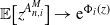 $\mathbb{E}\big[z^{A^M_{n,i}}\big] \rightarrow \mathrm{e}^{\Phi_i(z)}$
, where
 $\Phi_i(z)=-\sum_{j \neq i}\mathbb{E}\left[1-z^{h_{i,j}(\tilde{X_i})\textbf{1}_{\left\{U<\sigma_i\left(\tilde{X}_i\right)\right\}}}\right]$
. Therefore,
 \begin{equation*}\mathbb{E}\big[z^{A^M_{n,i}}\big] \rightarrow \exp\left\{-\sum_{j \neq i}\left(1-\mathbb{E}\left[z^{h_{i,j}\left(\tilde{X}_i\right)\textbf{1}_{\left\{U<\sigma_i\left(\tilde{X}_i\right)\right\}}}\right]\right)\right\}.\end{equation*}
This expression is of the form (8), which proves Lemma 11.
We now prove Theorem 3.
Proof of Theorem 3. We use the same reasoning as previously.
Lemma 2 still holds (the replicas are still exchangeable, only the nodes are not). Lemma 10 replaces Lemma 3. Since the functions
 $g_{1,i}$
and
 $g_{2,i}$
only depend on the node and not on the replica index, an equivalent result to Lemma 8 still holds. Lemma 5 is replaced by Lemma 11. For asymptotic independence, we have, using the same arguments as in the proof of Lemma 6, for
 $u,v \in [0,1]$
,
 $n \neq m$
, and
 $i \neq j$
,
 \begin{multline*}\!\!\!\!\mathbb{E}\big[u^{A^M_{n,i}}v^{A^M_{m,j}}\big] \rightarrow \exp\left\{-\sum_{i' \neq i}\left(1-\mathbb{E}\left[u^{h_{i,i'}(\tilde{X}_i)\textbf{1}_{\{U<\sigma_i(\tilde{X}_i)\}}}\right]\right)-\sum_{j' \neq j}\left(1-\mathbb{E}\left[v^{h_{j,j'}(\tilde{X}_j)\textbf{1}_{\{U<\sigma_i(\tilde{X}_j)\}}}\right]\right)\right\} \end{multline*}
when
 $M \rightarrow \infty$
. The other cases (
 $n=m$
and
 $i=j$
) are also valid. Lemma 7 also still holds, with only minor differences in the limit expressions.
Note that once again, this proves that the limit processes
 $\tilde{\hat{X}}_i$
and
 $\tilde{A}_j$
are independent for all
 $i,j \in \{1,\ldots,K\}$
.
As an application, let us apply this result to the model from Section 2 with the addition of nonexchangeable interactions. Namely, we consider
 $h_{i,j}\big(X^M_{m,j}\big)=\mu_{i,j}$
with
 $\mu_{i,j} \in \mathbb{N}$
(potentially zero). In this case, Theorem 3 proves the propagation of chaos in this system, and the limit distributions of arrivals at the different nodes are characterized by, for
 $i \in \{1,\ldots,K\}$
and
 $z \in [0,1]$
,
 \begin{equation*}\mathbb{E}\big[z^{\tilde{A}_i}\big] = \exp\Bigg\{\theta_i\sum_{j \neq i}\left(z^{\mu_{i,j}}-1\right)\Bigg\} = \prod_{j \neq i} \mathrm{e}^{\theta_i\left(z^{\mu_{i,j}}-1\right)},\end{equation*}
where
 $\theta_i=\mathbb{E}\big[\sigma_i(\tilde{X}_i)\big]$
. Note that, as expected, when all
 $\mu_{i,j}$
are equal to one, we obtain the result from Section 2.
6. Extensions
There are several ways of extending the FIAP framework while preserving the basic properties proved in the present paper (propagation of chaos and the Poisson hypothesis). We decided not to include them in the general framework in order to keep the notation and exposition light. A few natural extensions of this type are nevertheless discussed below.
6.1. Random interactions
The functions
 $h_{i,j}(k)$
can be replaced by randomized functions of the type
 $h_{i,j}(k,V_{i,j})$
, where the random variables
 $\{V_{i,j}\}_{1\le i,j\le K}$
are i.i.d. uniformly in [0, 1]. This allows us to represent, e.g., the queueing theory scenario where a customer leaving a queue is randomly routed to an other queue of the network according to some stochastic routeing matrix
 $\{p_{j,i}\}_{1\le i,j \le K}$
, namely a customer leaving queue i is routed to queue j with probability
 $p_{j,i}$
. If the random variables
 $\{V_{i,j}\}$
are independent of
 $\{X_i\}_i$
, then the main results still hold.
6.2. Time-inhomogeneous dynamics
The general setting of the paper implicitly suggests using the same (activation, fragmentation, and interaction) functions at all time steps for a given node. There is no difficulty extending the results to the time-inhomogeneous case where these functions depend on the time step. In the neural network case, this for instance happens in certain learning dynamics where the synaptic weights evolve over time.
6.3. Exogenous input and output
To the endogenous arrivals
 $A_i$
to node i given in (2) we add arbitrary exogenous arrivals
 $B_i\in \mathbb N$
. In the special case where the random variables
 $\{B_i\}$
are independent, Poisson, and independent of the state variables
 $\{X_i\}_i$
then the same results still hold. Note that we can also define an exogenous output for node i through the relation
 $D_i= h_{o,i} (X_i) \textbf{1}_{\{U_i<\sigma_i(X_i)\}}$
, where
 $h_{o,i}$
is a given output function
 $\mathbb N\to \mathbb N$
.
Exogenous input point processes are needed for modeling reasons in a variety of contexts (e.g. to represent requests from end-users in a computer network, or input signals from sensors in a neural network). Exogenous output processes are useful in, e.g., a two-layer network where the first layer feeds the second one, but not conversely. Exogenous input and output point processes are instrumental in the partition scheme of the vector state example discussed below. In that example, the exogenous input variables are neither necessarily Poisson nor independent.
6.4. Vector state example
This extension is first described through a simple neural network example. We partition the set of neurons of a discrete Galves–Löcherbach network in pairs (this assumes that K is even). Each pair of the partition is a node of the network. If (i,j) is one of these nodes, it has a two-dimensional vector state
 $(X_i,X_j)$
(rather than a one-dimensional state as in the initial model). We let this pair (as well as each other pair in the partition) evolve as a two-node GL network with some vector exogenous input and output. More precisely, conditionally on
 $(X_i,X_j)=(k,l)$
, neurons i and j spike independently with probability
 $\sigma_i(k)$
and
 $\sigma_j(l)$
respectively. If none of them spikes, the state
 $(Z_i,Z_j)$
after its endogenous evolution is still
 $(X_i,X_j)$
. If only i (resp. j) spikes and the other neuron of the pair does not spike, then
 $(Z_i,Z_j)$
is equal to
 $(0,X_j+r_{j,i})$
(resp.
 $(X_i+r_{i,j},0)$
). If both spike, then
 $(Z_i,Z_j)=(r_{i,j},r_{j,i})$
, with
 $r_{k,l}$
equal to 1 if there is a directed edge from l to k and 0 otherwise. Therefore, if
 $(B_i,B_j)$
denotes the vector exogenous input, the state of this pair at time one is
 $(Z_i+B_i,Z_j+B_j)$
, by combining the endogenous evolution and the exogenous arrivals.
Define now the exogenous output of type
 $k\notin \{i,j\}$
of node (i,j) by
 $D_k(i,j)= \textbf{1}_{\{U_i<\sigma_i(X_i)\}} r_{k,i} + \textbf{1}_{\{U_j<\sigma_j(X_j)\}} r_{k,j}$
. The extension of interest here involves taking the following exogenous input to node (i,j):
 \begin{equation*}B_i=\sum_{k\notin \{i,j\}} D_i(k,l(k))\textbf{1}_{\{k<l(k)\}}, \qquad B_j=\sum_{k\notin \{i,j\}} D_j(k,l(k))\textbf{1}_{\{k<l(k)\}},\end{equation*}
with l(k) the neuron paired with k.
Note that with this definition, when neuron i spikes, the effect on pair (k,l) with
 $l=l(k)$
is as follows: no effect if
 $r_{k,i}=r_{l,i}=0$
; one arrival in k and none in l (resp. one in l and none in k) if
 $r_{k,i}=1$
and
 $r_{l,i}=0$
(resp.
 $r_{l,i}=1$
and
 $r_{k,i}=0$
); a simultaneous arrival in both l and k otherwise. This defines a network which does not belong to the FIAP class, were it only because the state is now a vector. The M-RMF model features M replicas of this network with
 $K/2$
(vector state) nodes each. In this M-RMF model, the exogenous output of node/pair (i,j) in replica m is randomly sent to a replica chosen at random. More precisely, for all exogenous output type k paired with l,
 $D_k^m(i,j)= \textbf{1}_{\left\{U_i^m<\sigma_i\left(X^m_i\right)\right\}} r_{k,i} + \textbf{1}_{\left\{U^m_j<\sigma_j\left(X^m_j\right)\right\}} r_{k,i}$
(resp.
 $D_l^m(i,j)= \textbf{1}_{\left\{U_i^m<\sigma_i\left(X^m_i\right)\right\}} r_{l,i} + \textbf{1}_{\left\{U^m_j<\sigma_j\left(X^m_j\right)\right\}} r_{l,i}$
) units are sent to k (resp. l) of another replica selected uniformly at random where they are aggregated to the coordinates of the state variable of this pair. It can be shown that when M tends to infinity, (i) the random state vectors
 $\big(X^m_{i},X^m_{j}\big)$
and
 $\big(X^m_{i'},X^m_{j'}\big)$
, where (i,j) and (i’,j’) are two different pairs, are asymptotically independent (although the two coordinates of each vector are, in general, dependent); (ii) the exogenous arrivals to any coordinate of a pair in a typical replica tends to an independent compound Poisson variable.
6.5. Vector state general case
Consider a FIAP F with K nodes. Let
 $S_1,S_2,\ldots,S_l$
be a partition of
 $[1,\ldots,K]$
. Let
 $K_p$
,
 $1\le p\le l$
, denote the cardinality of set
 $S_p$
, and let
 $F_p$
be the restriction of F to the coordinates of
 $S_p$
. Let
 $\mathfrak{F}_p$
be the FIAP combining the endogenous dynamics of
 $F_p$
and exogenous input
 $(\mathfrak{B}_{p,i},\ i\in S_p)$
. Let
 $\mathfrak{X}_{p,i}$
denote the state variables in
 $\mathfrak{F}_p$
. For all
 $k\notin S_p$
, define the exogenous output of type k of
 $\mathfrak{F}_p$
as
 \begin{equation}\mathfrak{D}_p(k)= \sum_{i\in S_p}\textbf{1}_{\{U_{p,i}<\sigma_i(\mathfrak{X}_{p,i})\}} h_{k,i}(\mathfrak{X}_{p,i}).\end{equation}
Note that
 $\mathfrak{D}_p(k)$
is also what coordinate k receives as exogenous input from
 $S_p$
. That is, if we take
 \begin{equation}\mathfrak{B}_{p,i}=\sum_{q\ne p}\mathfrak{D}_q(i), \qquad i \in S_p,\end{equation}
we get another (more complex) representation of the dynamics of F based on the point processes describing the interactions between the sets of the partition. The M-RMF model associated with this partition features M replicas of this network with q (vector state) nodes each. In this M-RMF model, the exogenous output of node
 $i\in S_p$
of replica m is randomly sent to replicas chosen at random. More precisely, for all
 $q\ne p$
, the vector
 $(\mathfrak{D}_p^m(k),\ k\in S_q)$
, with
 $\mathfrak{D}_p^m(k)$
defined as in (9), is sent to one replica chosen at random, and this is done independently for all
 $q\ne p$
. This in turn defines new exogenous input point processes
 $\mathfrak{B}_{p,i}^m$
as in (10). Let
 $(\mathfrak{X}^m_{p,i},\ i\in S_p,\ p=1,\ldots,l,\ m=1,\ldots,M)$
denote the state variables in this M-RMF model. It can be shown that, when M tends to infinity,
-
(i) for all
$p\ne q$
, the random state vectors
$(\mathfrak{X}^m_{p,i},\ i\in S_p)$
and
$(\mathfrak{X}^m_{q,j},\ j\in S_q)$
are asymptotically independent (although the coordinates of each vector are, in general, dependent); -
(ii) for all p, and for all m, the exogenous arrivals
$(\mathfrak{B}^m_{p,i},\ i\in S_p)$
to set
$S_p$
tend to an independent multivariate compound Poisson variable with multivariate generating function In this last equation,
\begin{equation*} \exp\Bigg(\sum_{q\ne p} \sum_{n_i\in \mathbb N, i\in S_q} \sum_{s\subset S_q} \pi_{q,s,(n_i)}\Bigg( 1-\prod_{i\in s} \prod_{k\in S_q} z_k^{h_{k,i}(n_i)}\Bigg)\Bigg).\end{equation*}
where
\begin{equation*} \pi_{q,s,(n_i)}=\textbf{P} \big[\tilde{\mathfrak{X}}_{q,i}=n_i,\ i\in S_q\big]\prod_{j\in s} \sigma_j(n_j) \prod_{j'\in S_q{\setminus} s} (1-\sigma_{j'}(n_{j'})),\end{equation*}
$(\tilde{\mathfrak{X}}_{q,i})$
denotes random variables with the limiting joint distribution assumed in the vector generalization of PAI.


7. Conclusion
A new class of discrete-time dynamics involving point-process-based interactions between interconnected nodes was introduced. The Poisson hypothesis was proved for the RMF version of such dynamics. The proof is based on the property of pairwise asymptotic independence between replicas, and is by induction over time. The key point is that randomized routeing decisions on exchangeable events which are asymptotically independent lead to Poisson point processes. As for future research, a natural question is whether these results extend to continuous-time and continuous-space versions of FIAP dynamics. The extension to continuous-time FIAPs will follow from similar arguments to those presented here under the condition that the replica-limit/time-limit diagram commutes for FIAPs. The extension to continuous-space FIAPs appears to require analytical tools distinct from those presented here. Finally, another question of interest is whether the Poisson hypothesis can be shown for the RMF limits of other classes of systems besides FIAPs.
Acknowledgements
The authors would like to thank N. Gast, S. Rybko, S. Shlosman and the anonymous referees for their comments on the present paper.
Funding Information
T.T. was supported by the Alfred P. Sloan Research Fellowship FG-2017-9554. F.B. was supported by an award from the Simons Foundation (#197982). Both awards are to the University of Texas at Austin. F.B. and M.D. were supported by the ERC NEMO grant (#788851) to INRIA Paris.
Competing Interests
There were no competing interests to declare which arose during the preparation or publication process of this article.


