




No CrossRef data available.
ASYMPTOTIC INFERENCE FOR UNIT ROOT PROCESSES WITH GARCH(1,1) ERRORS
Published online by Cambridge University Press: 06 June 2003
Abstract
This paper investigates the so-called one-step local quasi–maximum likelihood estimator for the unit root process with GARCH(1,1) errors. When the scaled conditional errors (the ratio of the disturbance to the conditional standard deviation) follow a symmetric distribution, the asymptotic distribution of the estimated unit root is derived only under the second-order moment condition. It is shown that this distribution is a functional of a bivariate Brownian motion as in Ling and Li (1998, Annals of Statistics 26, 84–125) and can be used to construct the unit root test.The authors thank the co-editor, Bruce Hansen, and two referees for very helpful comments and suggestions. W.K. Li's research is partially supported by the Hong Kong Research Grants Council. Ling's research is supported by RGC Competitive Earmarked Research grant HKUST6113/02P.
Information
- Type
- Research Article
- Information
- Copyright
- © 2003 Cambridge University Press
1. INTRODUCTION
Consider the unit root process with the first-order general conditional heteroskedastic errors [GARCH(1,1)]:


where φ = 1 and α0 > 0, α ≥ 0, and β ≥ 0, and ηt's are a sequence of independently and identically distributed (i.i.d.) random variables with zero mean and variance one.
The GARCH models were proposed by Bollerslev (1986) and have important applications in financial and econometric time series. Some reviews can be found in Bollerslev, Engle, and Nelson (1994). When α = β = 0, εt's defined by model (1.2) reduce to i.i.d. white noises, and in this case the unit root process has been investigated for a long time. In recent decades, motivated by the practical applications in statistics and econometrics, many statisticians and econometricians have considered various unit root processes with non-i.i.d. errors. Some related results on estimating and testing unit roots can be found in Phillips and Durlauf (1986), Phillips (1987), Chan and Wei (1988), Lucas (1995), and Herce (1996) and references therein. When the error terms follow a GARCH model, how to estimate and how to test the unit root are obviously important problems.
Ling and Li (1998) derive the limiting distribution of the local maximum likelihood estimator (MLE) for a general nonstationary autoregressive moving-average time series with general-order GARCH errors and demonstrate that the MLE is more efficient than the least squares estimator (LSE). Seo (1999) also independently has derived the limiting distribution of the local MLE unit root in the nonstationary AR(p) model. The simulation results in Seo (1999) and Ling, Li, and McAleer (2001) show that the unit root tests based on the MLE are not only more powerful than Dickey–Fuller tests based on the LSE but also have more stable sizes. However, the results in Ling and Li (1998) require that Eεt4 < ∞, whereas those in Seo (1999) require that Eεt8 < ∞.
Note that the condition for strict stationarity is ln(αηt2 + β) < 0 (see Nelson, 1990), the condition for Eεt2 < ∞ is α + β < 1, and the condition for Eεt4 < ∞ is 3α2 + 2αβ + β2 < 1. The conditions for Eεt4 < ∞ or Eεt8 < ∞ are clearly much more stringent. For the pure GARCH(1,1) model, Lee and Hansen (1994) and Lumsdaine (1996) prove that MLE are consistent and asymptotically normal under ln(αηt2 + β) < 0. A challenging problem is whether or not we can derive the limiting distribution of the MLE under weaker conditions for the unit root process with GARCH errors. When ηt is symmetrically distributed, in this paper we obtain the asymptotic distribution of the so-called one-step local quasi-MLE of the unit root in model (1.1) under the assumption that α + β < 1, that is, only the existence of the second moment of εt is required. In the literature on unit root with GARCH, this is the weakest condition for the unit root distribution to exist. This limiting distribution is a functional of a bivariate Brownian motion and is also the same as that obtained in Ling and Li (1998).
This paper proceeds as follows. Section 2 presents the one-step local MLE and main results. Section 3 extends the results in Section 2 to models with a constant intercept. The proof of main results is given in Section 4.
Throughout the paper, U′ denotes the transpose of the vector U; o(1)(op(1)) denotes a series of numbers (random numbers) converging to zero (in probability); O(1)(Op(1)) denotes a series of numbers (random numbers) that are bounded (in probability);

denote convergence in probability and in distribution, respectively; and D = D[0,1] denotes the space of functions f (s) on [0, 1], which is defined and equipped with the Skorokhod topology (Billingsley, 1968).
2. ONE-STEP LOCAL QMLE AND MAIN RESULTS
Given observations y1,…,yn with the initial value y0 = 0, generated by model (1.1), the log-likelihood function (ignoring a constant) can be written as

Assumption 1.

.
Assumption 2. ηt has a symmetric distribution and Eηt4 < ∞.
Because we do not assume that ηt is normal, the maximizer of

on R × Θ is called the quasi–maximum likelihood estimator (QMLE) of φ = 1 and δ. In practice, ε0 and h0 are unavailable and can be replaced by some constants. These initial values do not affect our asymptotic results, which can be verified via some arguments similar to those in Lee and Hansen (1994).
Let

be the LSE of the unit root φ = 1 in model (1.1). Then

. The residual

can be used as the artificial observations of εt to estimate δ in model (1.2) through MLE as in Lee and Hansen (1994). Because

[see (2.9), which follows], Theorem C in Appendix C shows that Hessian matrices based on

are asymptotically equivalent. The corresponding asymptotic equivalence on the log-likelihood functions and the score functions can be found in Lemma 2.1 in Ling et al. (2001). Thus, if Assumptions 1 and 2 hold then the MLE of δ based on

is asymptotically equivalent in probability to that based on the true εt as in Lee and Hansen (1994). Hence, we assume that the estimator

δn of δ has been obtained and

.
Using

and an initial estimator

with

, the one-step local QMLE of φ = 1, denoted by

, is obtained by the one-step iteration

When

, we abbreviate

, respectively. If Assumptions 1 and 2 hold, then

by Lemma 6.5 in Ling et al. (2001), and hence, by Theorem 3.1 in the same paper, we have


uniformly in the ball Θn = {φ : |n(φ − 1)| ≤ M} for any fixed positive constant M. Thus, by (2.2)–(2.4), we have that

As pointed out by a referee and the co-editor Professor Bruce Hansen,

is not the local QMLE in the usual sense, but it has the same asymptotic distribution as the QMLE. We call

the one-step QMLE. In practice, we can use

as a new initial value to repeat the iterative procedure (2.2), and, for the estimated value from each iterative procedure, it has the same asymptotic representation as (2.5). The following is our main result.
THEOREM 2.1. Let

be the estimator of the unit root φ = 1 such that (2.5) holds. If Assumptions 1 and 2 are satisfied, then

where (w1(τ),w2(τ)) is a bivariate Brownian motion with covariance


. In particular, when ηt is normal, κ = 2.
Remark. Let

where σ2 = Eht and K is the (2,2)th element of Ω in (2.6). Then B1(τ) and B2(τ) are two independent standard Brownian motions. As shown in Ling and Li (1998),

The second term of (2.7) can be simplified as

, where ξ is a standard normal random variable independent of

(see Phillips, 1989). Let

. We can obtain that

Under Assumptions 1 and 2, Ling et al. (2001) show that

From (2.8) and (2.9), we see that the asymptotic distribution of

is a combination of that of

and a scale mixture of normals. This property is similar to those of the least absolute deviation estimators of unit roots given by Herce (1996). Ling and Li (1998) show that

is more efficient than

, in the sense defined in Ling and McAleer (2003). Our result heavily relies on the symmetry assumption. When ηt is asymmetric, the MLEs of φ and δ are not asymptotically independent, and hence (2.4) and (2.5) do not hold. In this case, the limiting distribution of the local MLE of (φ,δ) can be obtained by using a similar method to that in Ling and McAleer (2003).
3. MODELS WITH A CONSTANT INTERCEPT
The co-editor, Bruce Hansen, pointed out that many economic data include an intercept. In this section, we consider the following model:


where δ = (α0,α,β) is defined as in (2.1). Denote λ = (μ,φ)′ and assume that its true value is λ0 = (0,1)′. Let

be the LSE of λ0. Then

Let the residual

. Under Assumptions 1 and 2, Ling et al. (2001) prove that the MLE of δ based on

is asymptotically equivalent in probability to that based on the true εt as in Lee and Hansen (1994). As in Section 2, we can assume that the estimator

of δ has been obtained and

.
The log-likelihood function for model (3.1) and (3.2) is similarly defined as (2.1) with φ replaced by λ. Let

. Using an initial value

with

, the one-step local QMLE

of λ0 is obtained by the one-step iterative procedure as (2.2) with φ replaced by λ. If Assumptions 1 and 2 hold, then

by Lemma 6.5 in Ling et al. (2001), and hence, by Theorem 3.1 in the same paper, we can obtain the asymptotic representation

In Appendix B, we show that

Thus, by Theorem 2.1, Lemma 4.2 in the next section, (3.5), and the continuity mapping theorem, we have the following result.
THEOREM 3.1. Let

be the estimator of λ0 = (0,1)′ such that (3.4) holds. If Assumptions 1 and 2 hold, then

where F and (w1(τ),w2(τ)) are defined as in Theorem 2.1.
Remark. Similar to (2.8), by Theorem 3.1, we can show that
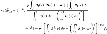
where c and ρ are defined as in (2.8). Under Assumptions 1 and 2, Ling et al. (2001) show that

From (3.6) and (3.7), we see that the limiting distribution of

is a combination of that of

and a scale mixture of normals. Some critical values of limiting distributions in (2.8) and (3.6) with different ρ are given in Ling et al. (2001), and those for the corresponding t-statistics are given in Seo (1999) and Ling et al. (2001).
4. PROOF OF MAIN RESULTS
LEMMA 4.1. Under Assumption 1, the processes ht and εt defined by model (1.2) are strictly stationary and ergodic and have the expansions

and

Proof. This comes straightforwardly from Theorem 2 in Nelson (1990) (for another expansion, see also Ling and Li, 1997). █
LEMMA 4.2. Suppose that the process εt is generated by model (1.2) and Assumptions 1 and 2 are satisfied. Then

where [w1(τ),w2(τ)] is a bivariate Brownian motion with mean zero and covariance τΩ and Ω is defined in Theorem 2.1.
Proof. Let λ = (λ1,λ2)′ be a constant vector with λλ′ ≠ 0. Denote

By Lemma 4.1, it is easy to show that both ξt and ξt* are martingale differences with respect to

, where

is the σ-field generated by {ηt,ηt−1,…}. First we consider the asymptotic property of

. From Lemma 4.1, we see that ht is a function in terms of {ηt−12, ηt−22,…}. Note that

and ηt is symmetric. It is easy to see that E(εt−iεt−j /ht2) = 0 as i ≠ j, and hence

where σ2 = Eht. By Assumption 2 and the Cauchy–Schwarz inequality, σ2E(1/ht) > 1 and hence σ*2 > λ1σ2 + 2λ1λ2 + λ22E(1/ht) = (σλ1 + λ2 /σ)2 + λ22[σ2E(1/ht) − 1]/σ2 > 0. Note that

By Lemma 4.1,

is a strictly stationary and ergodic time series. By the ergodic theorem and Assumption 2, it is easy to show that

Furthermore, because {ξt*} is also a strictly stationary and ergodic time series with finite variance, it follows that, for any small ε > 0,

as n → ∞, where P(x) is the distribution function of ξt*. By (4.3) and (4.4) and the invariance principle for martingale (Hall and Heyde, 1980, Theorem 4),

where W*(τ) is a Brownian motion with variance σ*2τ.
Let

. Note that

where c is a constant and o(1) holds uniformly in τ ∈ [0,1] . By (4.5) and (4.6),

Furthermore, by Cramér's device, we complete the proof. █
LEMMA 4.3. Suppose that Assumption 1 holds. Then:

Proof.

LEMMA 4.4. Suppose that Assumptions 1 and 2 hold and gt is one of the following types of random variables:

Then

converges to a constant σ02 and

where w0(τ) is a standard Brownian motion.
Remark. Davis, Mikosch, and Basrak (1999) prove that εt and ht are strongly mixing with geometric rates. As a referee pointed out, it is possible to prove Lemma 4.4 under some mixing framework. However, one has not shown in the literature that

, which follow, are strongly mixing. Our proof uses Theorem 21.1 in Billingsley (1968) and heavily relies on Lemma 4.1.
Proof. Because the proofs of (a) and (b) are similar, we present only the proofs of (b) and (c). For (b), denote

where εt,l, ht,l, and εt−k,l are defined as in Lemma 4.3. By Lemma 4.1, gt* is a measurable function of ηt,ηt−1,…. Meanwhile gt,l* is a measurable function of {ηt,…,ηt−l}.

In Appendix A, we prove that there exists a ρ ∈ (0,1) such that

By (4.7) and (4.8), it is easy to show that

By Theorem 21.1 in Billingsley (1968),

converges absolutely to a constant σ02 and when σ0 > 0,

When σ0 = 0, it is not difficult to verify that the conditions C1–C4 of Theorem 3.2 in Ling and Li (1998) are satisfied and by the theorem,

Using a similar method as for (4.8), we can show that E(gt − gt*)2 = O(ρt) and hence

, where op(1) holds uniformly in τ ∈ [0,1] . Furthermore, by (4.10) and (4.11), we can claim that the conclusion with case (b) holds.
For case (c), let

Because 1 − 2εt2/ht = 1 − 2εt,l2/ht,l = 1 − 2ηt2 is independent of

, it follows that

where c is some constant. In Appendix A, we prove that there exists a constant ρ ∈ (0,1) such that

By (4.12) and (4.13), we have that

Similar to (b), we can complete the remaining proof of case (c). This completes the proof. █
LEMMA 4.5. (Ling and Li, 1998, Theorem 3.1). Let {Sn(τ),0 ≤ τ ≤ 1} and {ξk,k = 1,2,…} be two sequences of random processes such that

and almost all trajectories of S(τ) and ξ(τ) are continuous. Then

LEMMA 4.6. Let gt be defined as in Lemma 4.4. Then under Assumptions 1 and 2,

Proof. It is not difficult to verify that gt's satisfy the conditions (c) and (d) in Lemma 4.5 (see Ling and Li, 1998, the proof of Theorem 3.4). By Lemma 4.2 and the continuity mapping theorem,

. By Lemmas 4.4 and 4.5,

. This completes the proof. █
The following lemma gives the asymptotic properties of the information matrix.
LEMMA 4.7. Under Assumptions 1 and 2,

where F and w1(τ) are defined as in Theorem 2.1.
Proof.

Note that

Denote rt,i =

. Then Ert,i2 = i. We first study I2t in (4.14). By (4.15),

By Lemma 4.3(1)(b),

where o(·) holds uniformly in t. Similarly, we can show that the following equation holds uniformly in t:

By (4.16) and (4.18), we know that

Next, we show that

Because their proofs are similar, we prove only the latter.

Similar to Lemma 4.2, we can show that

where W(τ) is a Brownian motion. Similar to the proof of Lemma 4.6, by (4.22) and Lemma 4.5, it is easy to show that

Similar to (4.17), by Lemma 4.3(1)(b),

By (4.21), (4.23), and (4.24), it follows that

By (4.14), (4.19), and (4.20), we have

where the last equation holds by Lemma 4.6. Furthermore, note that

where the last equation holds because yt−12/n = Op(1) and εt−i2/ht = O(βi) a.s. Thus we have

by Lemma 4.2 and the continuity mapping theorem. This completes the proof. █
LEMMA 4.8. If Assumptions 1 and 2 hold, then

where (w1(τ),w2(τ)) is defined as in Theorem 2.1.
Proof.

where rt,i =

. Denote the last term in (4.27) as Rt. Similar to (4.24), we can show that

. Furthermore, by Lemma 4.2 and applying Theorem 2.2 in Kurtz and Protter (1991), we know that the conclusion holds. █
Proof of Theorem 2.1. By Lemma 4.2 and the continuity mapping theorem, all limiting distributions in Lemmas 4.7 and 4.8 are jointly convergent. By (2.5) and Lemmas 4.7 and 4.8, we complete the proof. █
APPENDIX A: PROOFS OF (4.8) AND (4.13)
Proof of (4.8). By the definition of εt−k,l in Lemma 4.3, |εt−k,l| ≤ |εt−k| a.s. Furthermore, by Lemma 4.3(1)(b), we have

Thus, by Lemma 4.3(2)(c),

where 0 < ρ < 1, ρ1 = max{β,ρ}, and 0 < ρ2 < 1 such that lρ1l < ρ2l for some large enough l.
By Lemma 4.3(2)(a),

Thus, by Lemma 4.3(2)(c),

where 0 < ρ < 1. By Lemma 4.3(1)(b),

where O(·) holds uniformly in all t. Hence

where 0 < ρ < 1. By (A.1)–(A.3), we complete the proof of (4.8). █
Proof of (4.13). Note that, by Lemma 4.3(1)(b),

Therefore

where c is a constant. By Lemma 4.3(1)(c), ht−k /ht < β−k a.s., and hence

Thus, by Lemma 4.3(2)(c),

where 0 ≤ ρ < 1, ρ1 = max{β,ρ}, and 0 < ρ2 < 1 such that l2ρ1l < ρ2l for some large enough l. By Lemma 4.3(2)(b) and 4.3(2)(c), the Cauchy–Schwarz inequality applying to ht−k /ht, and E [β/(αηt2 + β)]2 < 1, we have

where c is a constant. By (A.4)–(A.6), EL1t2 = O(ρl) with 0 < ρ < 1. Now, we consider L2t in (4.13).

where c is a constant. By Lemma 4.3(2)(a) and 4.3(2)(b), the Cauchy–Schwarz inequality, and E [β/ (αηt2 + β)]4 < 1,

where the second inequality follows by the Minkowski inequality. Similarly we can show that EL3t2 = O(ρl), where 0 < ρ < 1. This completes the proof of (4.13). █
APPENDIX B: PROOF OF (3.5)
Proof.

By (4.15),

By Lemma 4.3(1)(b),

where O(·) holds uniformly in t.

Similarly, we can show that

By (B.1)–(B.5), we have that

where the last equation holds by Lemmas 4.2, 4.4, and 4.5. Furthermore, note that

where the last equation holds because

Thus, we have that

by Lemma 4.2 and the continuity mapping theorem. This completes the proof. █
APPENDIX C: ASYMPTOTIC EQUIVALENCE OF HESSIAN MATRICES
The likelihood function based on εt can be written as

THEOREM C. Under Assumption 1, it follows that

Proof. For simplicity, we only consider the case with

. It is easy to modify the proof for the case with

.

When

. Because of the similarity, we only present the proof of the equation:

In the following discussion, all O(·), Op(·), and op(·) hold uniformly in

and t = 1,…,n.
Denote εt(φ) = yt − φyt−1. Because max1≤t≤n|n−1/2yt−1| = Op(1) under Assumption 1, it follows that εt(φ) = εt − [n(φ − 1)](n−1/2yt−1)n−1/2 = εt + Op(n−1/2). Thus,

By (C.3), we can show that

Note that

. By (C.3) and (C.4), it follows that

for i = 0,1,…, where the next to last equation holds because

. Again because

, we can show that

. Using the fact that

and a similar method as for (C.5), we can obtain

By (C.5), it is straightforward to show that

Similarly, by (C.6), we can obtain


By (C.7)–(C.9), it is easy to show that

Because

uniformly in

and any t and i, we have

where the last equation holds by (C.3). Similarly, it follows that

Note that

. By (C.11) and (C.12), we have

Taking ν1 small enough such that βlν1 > β, we have

Under Assumption 1, Eεt2 < ∞, and hence we can show that

. Note that εt2 = ηt2ht. By (C.13) and (C.14), we can show that

where 2ν < ν1. By (C.10) and (C.15), we have


By (C.5) and (C.13), it follows that

Finally, by (C.16)–(C.18), we can show that (C.2) holds. This completes the proof. █
References
REFERENCES
Billingsley, P.
(1968)
Convergence of Probability Measures.
New York:
Wiley.
Bollerslev, T.
(1986)
Generalized autoregressive conditional heteroskedasticity.
Journal of Econometrics
31,
307–327.CrossRefGoogle Scholar
Bollerslev, T.,
R.F. Engle, &
D.B. Nelson
(1994)
ARCH model. In
R.F. Engle and
D. C. McFadden (eds.),
Handbook of Econometrics,
vol. 4, pp.
2959–3038.
Amsterdam:
Elsevier Science.
Chan, N.H. &
C.Z. Wei
(1988)
Limiting distributions of least squares estimates of unstable
autoregressive processes.
Annals of Statistics
16,
367–401.CrossRefGoogle Scholar
Davis, R.A.,
T. Mikosch, &
B. Basrak
(1999)
The Sample ACF of Multivariate Stochastic Recurrence Equations with
Applications to GARCH.
Technical Report,
Laboratory of Actuarial Mathematics, University of Copenhagen.
Hall, P. &
C.C. Heyde
(1980)
Martingale Limit Theory and Its Applications.
San Diego:
Academic Press.
Herce, M.A.
(1996)
Asymptotic theory of LAD estimation in a unit root process with
finite variance errors.
Econometric Theory
12,
129–53.CrossRefGoogle Scholar
Kurtz, T.G. &
P. Protter
(1991)
Weak limit theorems to stochastic integrals and stochastic
differential equations.
Annals of Probability
19,
1035–1070.CrossRefGoogle Scholar
Lee, S.-W., &
R.E. Hansen
(1994)
Asymptotic theory for GARCH(1,1) quasi-maximum likelihood estimator.
Econometric Theory
10,
29–52.CrossRefGoogle Scholar
Ling, S. &
W.K. Li
(1997)
On fractionally integrated autoregressive moving-average time
series models with conditional heteroscedasticity.
Journal of the American Statistical Association
92,
1184–1194.CrossRefGoogle Scholar
Ling, S. &
W.K. Li
(1998)
Limiting distributions of maximum likelihood estimators for
unstable autoregressive moving-average time series with general
autoregressive heteroscedastic errors.
Annals of Statistics
26,
84–125.Google Scholar
Ling, S.,
W.K. Li, &
M. McAleer
(2001)
Estimation and testing for unit root processes with GARCH (1,1) errors:
Theory and Monte Carlo study.
Econometric Reviews
(special issue), forthcoming.Google Scholar
Ling, S., &
M. McAleer
(2003)
On adaptive estimation in nonstationary ARMA models with GARCH
errors.
Annals of Statistics 31,
forthcoming.Google Scholar
Lucas, A.
(1995)
Unit root tests based on M estimators.
Econometric Theory
11,
331–346.CrossRefGoogle Scholar
Lumsdaine, R.
(1996)
Consistency and asymptotic normality of the quasi-maximum
likelihood estimator in IGARCH(1,1) and covariance stationary
GARCH(1,1) models.
Econometrica
64,
575–596.CrossRefGoogle Scholar
Nelson, D.B.
(1990)
Stationarity and persistence in the GARCH(1,1) model.
Econometric Theory
6,
318–334.CrossRefGoogle Scholar
Phillips, P.C.B.
(1987)
Time series regression with a unit root.
Econometrica
55,
277–301.CrossRefGoogle Scholar
Phillips, P.C.B.
(1989)
Partially identified econometric models.
Econometric Theory
5,
181–240.CrossRefGoogle Scholar
Phillips, P.C.B. &
S.N. Durlauf
(1986)
Multiple time series regression with integrated processes.
Review of Economic Studies
53,
473–495.CrossRefGoogle Scholar
Seo, B.
(1999)
Distribution theory for unit root tests with conditional
heteroskedasticity.
Journal of Econometrics
91,
113–144.CrossRefGoogle Scholar
 You have
Access
- 33
- Cited by