“All day the dust sifted down from the sky, and the next day it sifted down. An even blanket covered the earth…Every moving thing lifted the dust into the air: a walking man lifted a thin layer as high as his waist, and a wagon lifted the dust as high as the fence tops, and an automobile boiled a cloud behind it. The dust was long in settling back again.”
—John Steinbeck, The Grapes of Wrath (Reference Steinbeck1939, pp. 6, 4)
The American Dust Bowl, a prolonged ecological event characterized by drought, accelerated soil erosion, and severe dust storms, represents one of the most devastating environmental catastrophes in American history (Worster Reference Worster1979). During this crisis, which lasted throughout the 1930s, a series of dust storms ravaged the U.S. Great Plains, destroying land, property, and agricultural livelihoods; disrupting public services; and causing injury to health and nutrition (Carlson Reference Carlson1935; Hansen and Libecap Reference Hansen and Libecap2004; Hornbeck Reference Hornbeck2012). Recent literature indicates that early-life shocks such as these can radically change the course of human capability formation, and thus shape adult outcomes (Almond Reference Almond2006; Heckman Reference Heckman2007; Almond and Currie Reference Almond and Currie2011b; Bhalotra and Venkataramani Reference Bhalotra and Venkataramani2012). In light of this literature, the Dust Bowl's shocks to health and incomes would be expected to have non-negligible adverse effects on wellbeing in later-life; however, these long-run human costs have been little studied, meaning we may currently underestimate the full toll of this important event in American history.Footnote 1
Accordingly, the aim of this paper is to analyze the long-term consequences of the Dust Bowl for the human capital of the children who lived through it. To do this, I take a difference-in-differences approach, using plausibly exogenous variation in childhood Dust Bowl exposure to explain variation in human capital in adulthood. Specifically, I draw on a sample of more than four million individuals who were born between the years 1900 and 1959 in 15 Great Plains and adjacent states, and who were enumerated as adults in the 1980–2000 U.S. Censuses. These IPUMS microdata offer rich individual-level information on a range of human capital outcomes, including educational attainment and later-life disability (Ruggles, Alexander, Genadek, et al. Reference Ruggles, Trent Alexander and Genadek2010). Each individual in the sample is then assigned a measure of Dust Bowl exposure in early life. The temporal component of childhood Dust Bowl exposure arises from cohort membership: of this sample, 1918–1941 birth cohorts were exposed to the Dust Bowl either as children or in utero, and are considered to have been treated. This cohort variation in Dust Bowl eligibility is then interacted with spatial variation in the severity of the Dust Bowl in the state of birth, proxied by measures of Dust Bowl-induced soil erosion taken from Richard Hornbeck (Reference Hornbeck2012).
Using these data, I test for the degree to which this natural disaster scarred human capital in the long run, the developmental pathways through which such scarring occurred, and the capacity for investment in human capital—here, in the form of New Deal-era public spending—to remediate the shock. I find that exposure to the Dust Bowl in childhood had statistically significant and economically meaningful adverse impacts on later-life outcomes, for instance, increasing disability and reducing fertility and college completion. I show that the results hold even after accounting for the possibly confounding effects of the Great Depression, migration, selective fertility, and selective mortality. Many of the worst adverse effects are found amongst those exposed prenatally and in early childhood, suggesting that congenital complications in capability development, together with low parental incomes in utero and thereafter, may be to blame for such later-life disadvantage. Lastly, results—especially those concerning New Deal spending—indicate that post-shock investment had the capacity to compensate for damage to child endowments.
This study makes two main contributions. First, it enriches our understanding of the Dust Bowl. The Dust Bowl's impacts on land management and conservation, agricultural recovery, and migration have been well studied, and qualitative sources on the Dust Bowl's short-term health effects abound (see, e.g., Worster Reference Worster1979; Helms, Pavelis, Argabright, et al. Reference Helms, Pavelis and Argabright1996; Hansen and Libecap Reference Hansen and Libecap2004; Cunfer Reference Cunfer2005; Fishback, Troesken, Kollmann, et al. Reference Fishback, Troesken, Kollmann, Libecap and Steckel2011; and Hornbeck Reference Hornbeck2012). While two recent studies, David Cutler, Grant Miller, and Douglas Norton (Reference Cutler, Miller and Norton2007) and Price Fishback and MelissaThomasson (Reference Fishback and Thomasson2014), have examined the impact of early-life exposure to a bundle of 1930s-era shocks on wellbeing in adulthood, to my knowledge, no existing study has attempted to quantify the long-term human costs of this natural disaster as separate from the larger macroeconomic shocks of the Great Depression.Footnote 2 As such, it is possible that the literature currently underestimates the damage caused by the Dust Bowl. By quantifying the event's later-life impact on human capital, I more fully account for its human toll.
Second, this article contributes to our understanding of the technology of human capital formation. By accounting for differences in the timing of Dust Bowl exposure, I provide suggestive evidence on both the channels by which adverse environmental shocks may affect different capabilities, and the sensitive periods for the development of these outcomes. More importantly, this study is one of few to examine the question of remediation. In contrast to household-level investment responses, which may be endogenous, here, the large-scale and plausibly exogenous compensatory investment represented by New Deal expenditure allows me to better test the extent to which children can bounce back from early-life deprivation. By showing that New Deal spending was effective in aiding recovery from Dust Bowl damage, I not only provide new historical evidence on this program's long-run impact, but I also provide new empirical evidence on the capacity for recovery from adverse shocks to a child's human capital endowment. In doing so, this study is one of the few in the capability formation literature that examines the contemporaneous public policy responses to disaster.
RELATED LITERATURE
During the period from 1930 to 1940, poor rainfall, high temperatures, and strong winds precipitated a series of massive dust storms across the U.S. Great Plains (Stephens Reference Stephens1937; Lord Reference Lord1938; Wallace Reference Wallace1938; Cunfer Reference Cunfer2005). These storms blew away roughly 480 tons of fertile topsoil per acre, with many regions losing more than 75 percent of their original topsoil by 1940 (Hansen and Libecap Reference Hansen and Libecap2004; Hornbeck Reference Hornbeck2012). Winds decimated existing crops through exposure and abrasion, and prevented new ones from being planted (Soil Conservation Service 1935). Meanwhile, dirt deposited downwind suffocated livestock and buried crops and property (Worster Reference Worster1979; Hansen and Libecap Reference Hansen and Libecap2004; Egan Reference Egan2006). Accordingly, agricultural yields were low (Bennett Reference Bennett1939; Bonnifield Reference Bonnifield1979) and recovery was slow (Hornbeck Reference Hornbeck2012).
The Dust Bowl was not just an environmental crisis, but a human tragedy as well. As the country struggled with the Great Depression, the Dust Bowl compounded misfortunes, especially for the farming communities of the Great Plains (Wallace Reference Wallace1938; Cutler, Miller, and Norton Reference Cutler, Miller and Norton2007). Economic hardship was widespread: meager harvests meant low incomes, nutritional deprivation, and, for some, farm foreclosure and migration (Bonnifield Reference Bonnifield1979; Worster Reference Worster1979). More directly, the drought could prove fatal (Fishback, Troesken, Kollmann, et al. Reference Fishback, Troesken, Kollmann, Libecap and Steckel2011), while poor air quality led to eye infections, influenza, and respiratory illnesses such as “dust pneumonia” (Soil Conservation Service 1935; Worster Reference Worster1979; Hurt Reference Hurt1981; Hansen and Libecap Reference Hansen and Libecap2004; Egan Reference Egan2006; Burns, Duncan, and Dunfey Reference Burns, Duncan and Dunfey2012). What was once home became surreal and terrifying, “as nearly a literal hell on earth as can be imagined” (Lord Reference Lord1938).
Research indicates that stress, deprivation, and early-life shocks to income and health can have long-term adverse impacts on wellbeing (Barker and Osmond Reference Barker and Osmond1986; Almond and Currie Reference Almond and Currie2011b). Human capital development may be impaired directly through childhood illness and deprivation, and indirectly, through poor prenatal conditions (e.g., maternal stress, illness, or malnutrition). These poor early-life circumstances hamper the successful development of capabilities such as cognitive and non-cognitive skills, metabolism, and immunity, and have been implicated in conditions from heart disease to schizophrenia (see the overview of the famine and fetal programming literatures in Cormac Ó Gráda Reference Ó Gráda2011).Footnote 3 In turn, low human capital stocks negatively impact other outcomes such as later-life income and employment (Heckman Reference Heckman2007; Bhalotra and Venkataramani Reference Bhalotra and Venkataramani2012). Given the Dust Bowl's well-documented destruction, Dust Bowl survivors are likely to suffer just such damage to human capital. It is this insight that motivates the following analysis.
EMPIRICAL APPROACH
Data
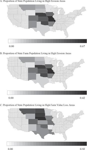
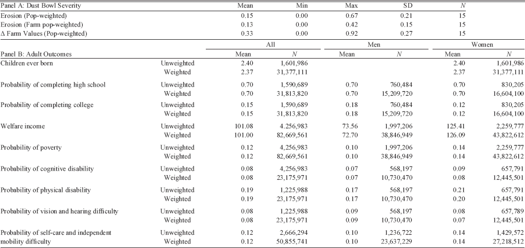
To measure the impact of early-life Dust Bowl exposure on later-life human capital, I draw from IPUMS a sample of individuals born between 1900 and 1959 in 15 Great Plains and adjacent states (see Figure 1), for whom we can observe stable human capital outcomes in adulthood. Specifically, I take data from the 5 percent samples of the 1980, 1990, and 2000 censuses, which provide detailed individual-level information on a range of human capital and wellbeing outcomes such as educational attainment, poverty, and the incidence of disability (Ruggles, Alexander, Genadek, et al. Reference Ruggles, Trent Alexander and Genadek2010). These particular census waves are chosen in part because they capture outcomes, such as educational attainment or completed fertility, which might not be stable until middle age; and outcomes, such as disability, which might not manifest until later in adulthood.Footnote 4 They are also chosen for the specific outcomes they contain. For instance, certain disability outcomes are available only in the 2000 census, while college and high school completion can only be calculated from the “highest grade completed” variable listed in 1980. Summary statistics on the adult human capital outcomes used in this study, by gender, are available in Table 1. Graphs of outcome summary statistics by gender and birth year, with 95 percent confidence intervals, are provided in Figures A1a–A1i in Section 4 of the Online Appendix.
DUST BOWL SEVERITY

SUMMARY STATISTICS

Note: Panel A reports summary statistics for state-level Dust Bowl severity measures. Erosion (pop-weighted) refers to the proportion of individuals in the state living in high-erosion counties in 1930. Erosion (farm pop-weighted) refers to the proportion of farm population in the state living in high-erosion counties in 1930. Change in farm values refers to the proportion of individuals in the state living in counties in 1930 that experienced high loss in farm values between 1930 and 1940. Panel B reports average values of human capital outcome variables by IPUMS observation (unweighted) and by IPUMS observation weighted by the IPUMS variable PERWT (weighted); the latter yields the average value of the human capital outcome variables for the entire population represented by the observations included.
Source: Panel A calculated from data in Hornbeck (Reference Hornbeck2012). Panel B calculated from the 5 percent IPUMS 1980, 1990, and 2000 samples (Ruggles, Alexander, Genadek, et al. Reference Ruggles, Trent Alexander and Genadek2010) for individuals born in 1900–1959, inclusive, in the 15 sample states given in Figure 1.
Using the year and state of birth listed in IPUMS, I assign each individual a measure of childhood exposure to the Dust Bowl. Temporal variation in Dust Bowl exposure comes from cohort membership. I consider an individual to have been treated by the Dust Bowl if they were a child at any point during the Dust Bowl. I take the Dust Bowl period to last from 1930–1940, and I define childhood as the ages –1 to 12 to capture the period in utero to the onset of puberty. Accordingly, those born 1918–1941 are taken as treated in the main analysis, while the remaining individuals, who were either too young or too old to have been children at the time of the Dust Bowl, serve as control cohorts. The inclusion of a range of different birth-year cohorts within each of the treated and control groups provides the variation necessary to disentangle age-at-exposure effects from cumulative (i.e., chronology-related) effects.
To identify the spatial component of Dust Bowl exposure during childhood, I use measures of soil erosion for 15 Great Plains and adjacent states (see Figure 1a) which account for 23 percent of U.S. population (U.S. Census Bureau Reference Census Bureau2002) and 47 percent of U.S. landmass (U.S. Census Bureau Reference Census Bureau2013) in 1930. Beyond what is typically thought of as the core Dust Bowl region, this group of states adds both similar nearby states in which there was relatively little damage, and states which are typically overlooked but which nevertheless suffered substantial erosion during the Dust Bowl.Footnote 5 Thus, this choice of states offers sufficient variation in erosion to enable analysis when erosion must be assigned at the birth-state level, which is the most granular level for which nativity information is available in the IPUMS data.
Erosion measures are taken from the U.S. Soil Conservation Service. Beginning in 1934 in response to the Dust Bowl, and continuing over its course, the Soil Conservation Service conducted comprehensive surveys of soil conditions across the United States, identifying thousands of areas of erosion classified by the severity (e.g., slight, moderate, severe) and type (e.g., sheet, wind, gullying) of damage observed (Soil Conservation Service 1935). By 1948, the office had created the first of a series of maps cataloging the cumulative erosion experienced over the full Dust Bowl period. I take my erosion figures from this cumulative erosion map (as reported in Richard Hornbeck Reference Hornbeck2012), which characterizes erosion severity by percentage of original topsoil lost: high (75 percent or more), medium (25–50 percent), and low (0–25 percent) erosion. To control for possible changes to county boundaries during the Dust Bowl period, per Hornbeck (Reference Hornbeck2012), 1910 county boundary definitions are enforced for measures of erosion, population, and farm value.
Since the severity of the Dust Bowl in human terms depends on population distribution over space within a given state, I weight erosion measures by population, taken from the U.S. Census, such that states with a greater proportion of population residing in high-erosion counties are deemed to have been more severely treated by the Dust Bowl. As an alternative means of weighting erosion, I also use measures weighted by the farm population.Footnote 6 Erosion measures are constructed at the state level so as to correspond to individual outcomes from IPUMS, which can only be measured at the birth-state level.Footnote 7
One limitation of the erosion data is the lack of baseline erosion measures, since no erosion surveys were made prior to 1934 (Soil Conservation Service 1935; Hornbeck Reference Hornbeck2012). To account for possible measurement error due to the absence of information on pre-1930 erosion levels, I substitute data from the U.S. Census of Agriculture on the percentage change in farm values between 1930 and 1940 for the erosion s term in equation (1) as a robustness check, since 1930 farm values proxy the quality of land prior to the Dust Bowl.Footnote 8 Maps detailing the severity of Dust Bowl exposure by measures of erosion and change in farm values are detailed in Figure 1.
Identification Strategy
I adopt a difference-in-differences approach, wherein plausibly exogenous environmental shocks to income and health—in the form of Dust Bowl-induced soil erosion—interact with cohort membership to impact later-life human capital. My baseline specification is as follows, and is estimated by ordinary least square (OLS):

Here, h ibst represents the later-life human capital outcome of interest for individual i born in year b in state s and observed in census year t. The term treated b × erosion s is the chief variable of interest, and refers to whether an individual was a child during the Dust Bowl and whether they were exposed to high erosion. It may thus be interpreted as the reduced form effect of childhood Dust Bowl exposure on adult outcomes. Treated b is equal to 1 for individuals aged –1 to 12 at any time during the Dust Bowl, so as to capture the effects of the shock during childhood, which has been defined so as to span the period in utero up to the onset of puberty.Footnote 9 Thus, in a sample comprising birth years 1900–1959, the Dust Bowl-treated cohort comprises children born 1918–1941. Erosion s represents the erosion intensity in a given state over the Dust Bowl period—that is, the degree of exposure to this random environmental shock. Since county-level erosion is known, but birth county is not, in the baseline, erosion s is constructed as the proportion of the state population in 1930 living in high-erosion counties within that state. Accordingly, it may be interpreted as the probability that an individual born in a given state was born into a high-erosion county. Since census data do not allow for the identification of those who may have migrated away from the birth state during childhood, the treated b × erosion s term may be interpreted as an intent-to-treat estimate. Thus, its coefficient, β 1, describes the causal effect of Dust Bowl exposure relative to those not exposed.
Finally, x ibst represents a vector of controls (in baseline, the individual's race; outside it, race, veteran status, and birth-state-birth-year per capita income), while θ s, λ b, η t, and γ bs represent birth-state fixed effects, birth-year fixed effects, census-year fixed effects, and linear birth-state trends, respectively. Together, these variables control for several dimensions of unobserved heterogeneity while also stripping away the effects of larger-scale trends in outcomes during this period, such that β 1 may be interpreted as the causal effect of Dust Bowl exposure above and beyond these phenomena.Footnote 10 Standard errors are two-way clustered by birth state and birth year so as to adjust for serial correlation in outcomes, and the equation is estimated separately for men and women to identify gender differences in Dust Bowl impacts.
For the purposes of identification, erosion must be plausibly exogenous, and the pre-trends in outcomes between high- and low-erosion birth states should be parallel. On the latter issue, comparisons of cohort trends in outcomes by above- and below-mean-erosion states indicate that parallel trends assumptions are upheld (not reported). Next, I elaborate on the former issue.
Although as an environmental phenomenon, we might expect that the Dust Bowl would be clearly exogenous, it could be endogenous if human activity exacerbated adverse weather conditions, or if individuals were selected into residence in the Great Plains. On the first point, although the contribution of Great Plains settlers to land degradation and dust storms has been long debated by scholars of the Dust Bowl (see, e.g., Worster Reference Worster1979 or Hansen and Libecap Reference Hansen and Libecap2004), more recent and in-depth analysis by Geoff Cunfer (Reference Cunfer2005) suggests that the Dust Bowl was largely driven by exogenous and cyclical climatic conditions and was not, as previous scholars have proposed and as had been popularly assumed, a man-made disaster. Thus, particularly when measured at the state level, it seems reasonable to treat the Dust Bowl as exogenous.
On the second point, we might worry that the Great Plains were settled by the poorest and most desperate farmers, who may have taken marginal lands and cultivated them sub-optimally. If this were the case, then we might expect that individuals born in more severely-stricken states were substantially more sensitive to Dust Bowl shocks because of their poverty, or that they were more prone to pursue farming strategies that depleted the land. However, there is no clear indication that erosion severity and pre-Dust Bowl poverty were strongly associated on the eve of the Great Depression: the correlation between Dust Bowl erosion and per capita personal income in 1929 is a relatively weak 0.29. Furthermore, the difference-in-differences design accounts for the pre-Dust Bowl period. That is, it naturally compares individuals born in Dust Bowl states before and after the shock to those born in Dust Bowl states during the shock. Thus, if Great Plains residents were adversely selected (say, due to nineteenth-century homesteading policies), then the inclusion in the (untreated) control group of individuals selected in the same manner as those who were treated, and using the same sorts of farming techniques as those treated, would help mitigate the concern over the endogeneity of Dust Bowl victims.Footnote 11 Lastly, after controlling, as I do, for state fixed effects and trends, it is unlikely that selective settlement or cultivation patterns in the lead-up to the 1930s would have effects on later-life outcomes except through the Dust Bowl.
MAIN RESULTS
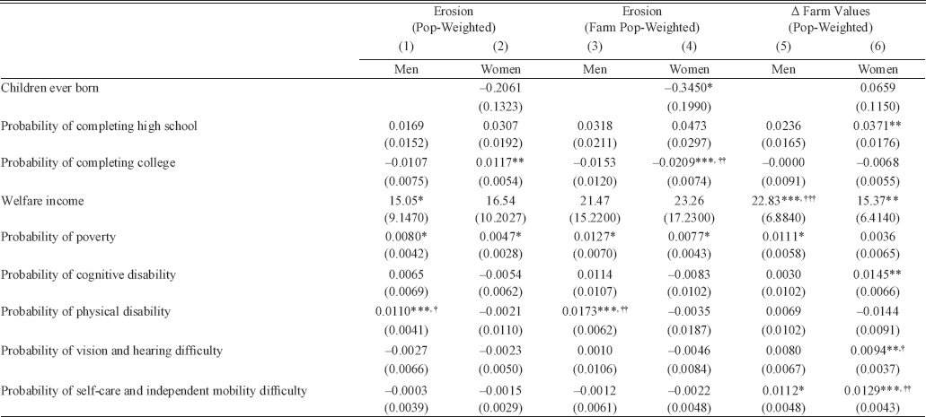
I begin by testing the impact of Dust Bowl exposure on later-life outcomes by sex.Footnote 12 Table 2 lists the estimates of β 1 from equation (1) for each of the later-life outcomes considered. I find that individuals exposed to the Dust Bowl as children suffered permanent damage to human capital and wellbeing on a scale that is both statistically and economically significant. Under the baseline specification in column (2), I find that exposed women had a 1.17 percentage point lower probability of completing college, and a 0.47 percentage point higher probability of living in poverty, defined as living at or below the census poverty line (see Section 2 of the Online Appendix). The poverty effects for men (column 1) are even starker: exposed men have a 0.80 percentage point greater likelihood of living in poverty than men who were not exposed, and receive $15.05 more in welfare payments. Furthermore, exposed men have a 1.10 percentage point greater chance of experiencing physical disability.
IMPACT OF CHILDHOOD EXPOSURE TO THE DUST BOWL ON LATER-LIFE OUTCOMES

*** p<0.01, ** p<0.05, * p<0.1 uncorrected.
††† p<0.01, †† p<0.05, † p<0.1 Bonferroni-corrected.
Note: Table reports treated b × erosion s coefficients. Each row in the left-hand column refers to the regression's dependent variable, while the remaining column headings indicate the definition of Dust Bowl severity (i.e., erosion s ) used. Treated cohorts are those born 1918–1941. All regressions are estimated by OLS and include controls for race; birth year, birth state, and census year fixed effects; and state trends. Standard errors, two-way clustered by birth state and birth year, are reported in parentheses below each coefficient.
Source: Erosion and farm value data are calculated from Hornbeck (Reference Hornbeck2012), while human capital outcome data come from the 5 percent IPUMS 1980, 1990, and 2000 samples (Ruggles, Alexander, Genadek, et al. Reference Ruggles, Trent Alexander and Genadek2010) for individuals born in 1900–1959, inclusive, in the 15 sample states given in Figure 1.
Columns (3) for men and (4) for women present the β 1 values for regressions in which the erosion s variable in equation (1) is instead defined as the proportion of the state's farm population (rather than total population) living in high-erosion counties (see Section 2 of the Online Appendix). In effect, these regressions test whether the Dust Bowl only mattered insofar as farmers were exposed: if a county hit by the Dust Bowl contained no farmers, it would not be considered exposed to the Dust Bowl, and would not contribute to the state's erosion level. Under this specification, exposed women see a fertility reduction of 0.35 children ever born, as well as a 2.09 percentage point decrease in the probability of completing college. The latter outcome is nearly twice as severe as in the baseline (i.e., total population-weighted erosion) specification. Exposed women are 0.77 percentage points likelier to be living in poverty than their unexposed counterparts; exposed men, 1.27 percentage points likelier. Exposed men similarly have a 1.73 percentage point increase in the probability of physical disability, a figure roughly 50 percent more severe than the in the baseline.
Finally, in columns (5) and (6), percentage change in farm values between 1930 and 1940 takes the place of erosion as the measure of Dust Bowl severity. As before, the measure is population-weighted. That is, I use the share of the population living in counties that experienced above-average losses in farm value over the 1930s. This farm-value-based measure is a useful exposure proxy since it does not penalize states that may naturally experience poor land quality or higher levels of pre-1930 erosion, traits that the baseline specification would attribute to the Dust Bowl. Here I find similar effects on poverty and welfare payments. However, a number of additional impacts are also statistically significant, most notably, disability: exposed men see a 1.12 percentage point greater chance of experiencing self-care and independent mobility disability, while exposed women experience 1.45, 0.94, and 1.29 percentage point increases in cognitive, vision and hearing, and self-care and independent mobility disabilities, respectively. Exposed women also see a 3.71 percentage point greater chance of high school completion than their unexposed counterparts. This seemingly counterintuitive finding (which also appears in the results in Tables 3–6 concerning developmental stage and public spending) may in fact reflect a drop in the opportunity cost of secondary schooling as farms, and thus, the demand for child farm labor, collapsed. I will return to this result in greater detail later on.Footnote 13
IMPACT OF EXPOSURE TO THE DUST BOWL BY DEVELOPMENT STAGE ON LATER-LIFE OUTCOMES: MEN

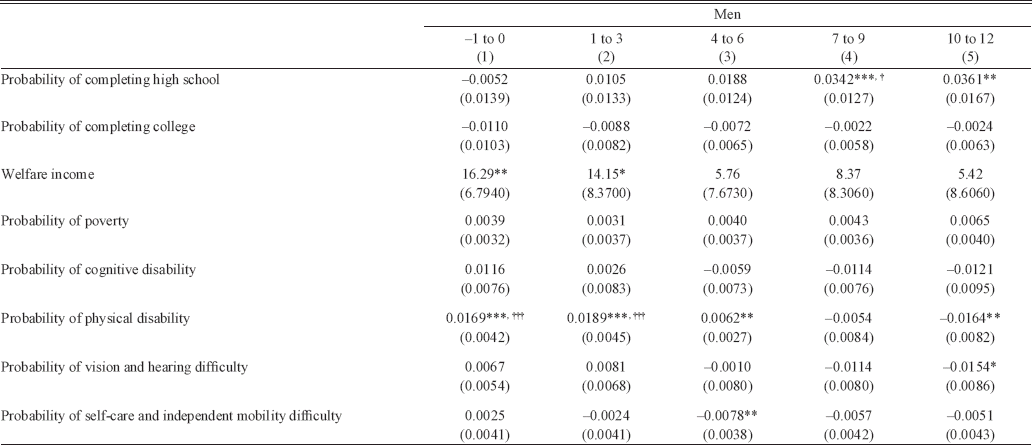
*** p<0.01, ** p<0.05, * p<0.1 uncorrected.
††† p<0.01, †† p<0.05, † p<0.1 Bonferroni-corrected.
Note: Table reports treated b × erosion s coefficients. Each row in the left-hand column refers to the regression's dependent variable, while the remaining column headings indicate the developmental stage that defines treated b. Treated b here is a duration-weighted measure that gives the proportion of time an individual born 1918–1941 spent in the given age band during the Dust Bowl years of 1930–1940 (see Section 2 of the Online Appendix). All regressions are estimated by OLS and include controls for race; birth year, birth state, and census year fixed effects; and state trends. Standard errors, two-way clustered by birth state and birth year, are reported in parentheses below each coefficient.
Source: Erosion data are calculated from Hornbeck (Reference Hornbeck2012), while human capital outcome data come from the 5 percent IPUMS 1980, 1990, and 2000 samples (Ruggles, Alexander, Genadek, et al. Reference Ruggles, Trent Alexander and Genadek2010) for individuals born in 1900–1959, inclusive, in the 15 sample states given in Figure 1.
IMPACT OF EXPOSURE TO THE DUST BOWL BY DEVELOPMENT STAGE ON LATER-LIFE OUTCOMES: WOMEN

*** p<0.01, ** p<0.05, * p<0.1 uncorrected.
††† p<0.01, †† p<0.05, † p<0.1 Bonferroni-corrected.
Note: Table reports treated b × erosion s coefficients. Each row in the left-hand column refers to the regression's dependent variable, while the remaining column headings indicate the developmental stage that defines treated b. Treated b here is a duration-weighted measure that gives the proportion of time an individual born 1918–1941 spent in the given age band during the Dust Bowl years of 1930–1940 (see Section 2 of the Online Appendix for details). All regressions are estimated by OLS and include controls for race; birth year, birth state, and census year fixed effects; and state trends. Standard errors, two-way clustered by birth state and birth year, are reported in parentheses below each coefficient.
Source: Erosion data are calculated from Hornbeck (Reference Hornbeck2012), while human capital outcome data come from the 5 percent IPUMS 1980, 1990, and 2000 samples (Ruggles, Alexander, Genadek, et al. Reference Ruggles, Trent Alexander and Genadek2010) for individuals born in 1900–1959, inclusive, in the 15 sample states given in Figure 1.
IMPACT OF EXPOSURE TO THE DUST BOWL BY MECHANISM: PUBLIC SPENDING - MEN

*** p<0.01, ** p<0.05, * p<0.1 uncorrected.
††† p<0.01, †† p<0.05, † p<0.1 Bonferroni-corrected.
Note: Tables report treated b × erosion s coefficients (columns a) and interaction×treated b × erosion s coefficients (columns b) for specifications that interact the baseline treatment term with the relevant measure of the state's total per capita New Deal and related spending. Treated cohorts are those born 1918–1941. All regressions are estimated by OLS and include two-way interactions and controls for race; birth year, birth state, and census year fixed effects; and state trends. Standard errors, two-way clustered by birth state and birth year, are reported in parentheses below each coefficient. Public spending variables are continuous; to aid in interpreting the interaction coefficient for these regressions, the minimum, maximum, and standard deviation for the relevant variables in the full sample are as follows: New Deal (104.351, 289.141, 47.396); Relief (41.708, 128.980, 23.143); Loans (58.462, 167.357, 23.787).
Source: Erosion data are calculated from Hornbeck (Reference Hornbeck2012), spending data are calculated from Fishback, Kantor, and Wallace (Reference Fishback, Kantor and Wallis2003), and human capital outcome data come from the 5 percent IPUMS 1980, 1990, and 2000 samples (Ruggles, Alexander, Genadek, et al. Reference Ruggles, Trent Alexander and Genadek2010) for individuals born in 1900–1959, inclusive, in the 15 sample states given in Figure 1.
IMPACT OF EXPOSURE TO THE DUST BOWL BY MECHANISM: PUBLIC SPENDING - WOMEN

*** p<0.01, ** p<0.05, * p<0.1 uncorrected.
††† p<0.01, †† p<0.05, † p<0.1 Bonferroni-corrected.
Note: Tables report treated b × erosion s coefficients (columns a) and interaction×treated b × erosion s coefficients (columns b) for for specifications that interact the baseline treatment term with the relevant measure of the state's total per capita New Deal and related spending. Treated cohorts are those born 1918–1941. All regressions are estimated by OLS and include two-way interactions and controls for race; birth year, birth state, and census year fixed effects; and state trends. Standard errors, two-way clustered by birth state and birth year, are reported in parentheses below each coefficient. Public spending variables are continuous; to aid in interpreting the interaction coefficient for these regressions, the minimum, maximum, and standard deviation for the relevant variables in the full sample are as follows: New Deal (104.351, 289.141, 47.396); Relief (41.708, 128.980, 23.143); Loans (58.462, 167.357, 23.787).
Source: Erosion data are calculated from Hornbeck (Reference Hornbeck2012), spending data are calculated from Fishback, et al. (Reference Fishback, Kantor and Wallis2003), and human capital outcome data come from the 5 percent IPUMS 1980, 1990, and 2000 samples (Ruggles, Alexander, Genadek, et al. Reference Ruggles, Trent Alexander and Genadek2010) for individuals born in 1900–1959, inclusive, in the 15 sample states given in Figure 1.
These results are intuitive, economically meaningful, and consistent with the literature on childhood shocks (e.g., Almond, Edlund, and Li, et al. Reference Almond, Edlund and Li2007; Banerjee, Duflo, Postel-Vinay, et al. Reference Banerjee, Duflo and Postel-Vinay2010; Ó Gráda 2010). The Dust Bowl had negative consequences for health, human capital, and indicators of wellbeing, increasing poverty and disability, and decreasing rates of college completion.Footnote 14 What is more, the long-run effects of the Dust Bowl on human capital appear to be on a similar scale to the event's short-run effects on land value.Footnote 15
MECHANISMS
Next, I investigate pathways through which the Dust Bowl may affect later-life outcomes. First, I test whether the types and severity of adverse effects are linked to the developmental stage at which children were exposed to the Dust Bowl. Second, I test for the effects of New Deal spending in ameliorating adverse effects on children's health, nutrition, and education. I report these results in Tables 3–6. Here, I show that many of the adverse effects outlined in the preceding section—for instance, lower rates of postsecondary education—appear to stem from low incomes and developmental complications in early life. Furthermore, I provide evidence that the New Deal was able to mitigate these environmental insults, suggesting that there is scope for compensating investments to remediate adverse shocks in early life.
Developmental Stage
To pinpoint the effects of the timing of exposure, I estimate equation (1) substituting the proportion of a given age band spent during the Dust Bowl period for the original treated b term. Thus, where all those aged –1 to 12 at any point between 1930 and 1940 would have been counted as treated on a binary basis, now each individual receives a duration-weighted measure of exposure during each development stage, defined as follows: –1 to 0 (in utero/neonatal), 1 to 3 (infancy), 4 to 6 (early childhood), 7 to 9 (school age), and 10 to 12 (early adolescence). See Section 2 of the Online Appendix for further discussion of development stage measures.Footnote 16
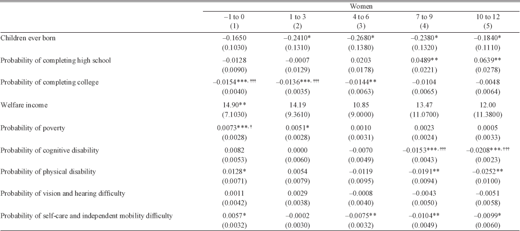
In Table 3, I report estimates of β 1 for men, and in Table 4, those for women.Footnote 17 I find that age at exposure matters, both to the severity and significance of adverse effects. Additionally, by disentangling the Dust Bowl's effects by developmental stage, these results provide suggestive evidence of likely pathways of impact that the baseline regressions obscure.
For men, adverse effects on poverty ($14.15–16.29 more in welfare receipts) and disability (1.69–1.89 percentage point higher rates of physical disability) are worst amongst those exposed in utero and in infancy. Adverse effects appear to dampen as the age of exposure rises,Footnote 18 except notably in disability outcomes; in the early adolescence period, shocks that in early childhood produced greater likelihoods of physical disability instead produce lower likelihoods of physical and vision and hearing disabilities.Footnote 19 These findings are consistent with the idea that congenital health defects (rather than, say, schooling disruptions) may be responsible for poor later-life outcomes and that these may act through disability, or even directly, to produce lower adult socioeconomic status.
For women, fertility outcomes are negatively affected across developmental stages. Exposed women experience a 0.18 to 0.27 child reduction in fertility, with the greatest adverse impact occurring in the 4 to 6 age range. That fertility reduction effects are greatest for those exposed to the Dust Bowl well before puberty suggests early damage to reproductive health, perhaps as an adaptive response to poor nutrition in the growing years. This interpretation is corroborated by the fact that exposed women had neither the higher marriage ages nor the higher college-completion rates associated with the deferral of childbearing in favor of long-term career planning (Goldin and Katz Reference Goldin and Katz2002), nor did they experience income levels in adulthood that might have induced them to voluntarily restrict fertility. This finding is particularly striking given the nationwide post-war “baby boom” trend in fertility experienced by the generation born in the 1920s and 1930s (see Figure A1a in Section 4 of the Online Appendix).
Meanwhile, as with men, it is in early childhood that exposed women's college completion, poverty, and disability effects are worst. Women exposed between the ages –1 and 6 had a 1.36–1.54 percentage point lower chance of completing college, with the greatest adverse effects accruing to those exposed in utero. A similar pattern follows for probability of poverty (0.73 percentage points higher for those exposed at ages –1 to 0 and 0.51 percentage points higher for those exposed at ages 1 to 3) and for physical disability and self-care and independent mobility difficulty (1.28 and 0.57 percentage points higher, respectively, for those exposed in utero). For both sexes, the preponderance of damage where exposure was in early childhood suggests that the pathway of impact is largely through subverted capability formation.Footnote 20
Public Spending Responses
Dynamic models of capability formation, such as that outlined in James Heckman (Reference Heckman2007), suggest that where the intertemporal elasticity of substitution in human capital investments is low, it may be very difficult to recover from early shocks to the human capital endowment. Remediation, then, is a matter for empirical study. However, the evidence base to date on the substitutability and complementarity of investments across periods is both limited and mixed (see reviews in Almond and Mazumder Reference Almond and Mazumder2013; Duque, Rosales, and Sanchez Reference Duque, Rosales and Sanchez2017; and Rossin-Slater and Wüst Reference Rossin-Slater and Wüst.2017). The 1930s famously saw the rollout of a series of New Deal-related spending programs—such as cash assistance, farm loans, and the building of schools, hospitals, and roads—that may have provided relief to Dust Bowl-stricken households. This raises an important question: although the results thus far make it clear that the Dust Bowl did have a statistically significant and economically meaningful adverse impact on the human capital of exposed individuals, could things have been even worse? Put another way, is there empirical support for the possibility of remediation in this setting? To examine this question, I test for whether New Deal spending attenuated the Dust Bowl's adverse effects.
I interact measures of total state-level per capita public spending over the period, taken from Price Fishback, Shawn Kantor, and John Wallis (Reference Fishback, Kantor and Wallis2003), with the measure of treatment as follows:

Depending on the specification, the public spending variable takes one of three values. The first is relief expenditure, which includes Works Progress Administration, Federal Emergency Relief Administration, and Public Assistance grants; the second is loans, which includes loans made in aid of farms and housing; and the third encompasses all New Deal expenditures, including additional expenditures such as those on the construction of roads and public buildings.Footnote 21 Evidence suggests that these state-level measures of New Deal-related spending may be treated as plausibly exogenous to Dust Bowl severity. For instance, I find these public spending variables to be largely uncorrelated with observable birth-state characteristics such as erosion. Additionally, panel regressions using annual state-level spending data for a variety of highly granular New Deal programs (Fishback Reference Fishback2015; Fishback and Kachanovskaya Reference Fishback and Kachanovskaya2015) indicate no significant relationship between spending and contemporaneous or lagged values of state drought or income per capita, except in the case of a few very narrow categories of relief spending (not reported). The apparent exogeneity of New Deal allocations to state-level need during the 1930s is consistent with Fishback, Haines, and Kantor (Reference Fishback, Haines and Kantor2007) and Fishback, Kantor, and Wallis (Reference Fishback, Kantor and Wallis2003), who suggest that funding may not have been allocated purely to severely-affected regions; rather, such spending may have in part been used to curry political favor. Although we might expect states that were more politically engaged, civic-minded, or public goods-oriented to receive more funding (and so, to enjoy different returns to or take-up of remediation efforts), the evidence on this is mixed. State-level spending appears to be weakly to moderately positively correlated with turnout in the 1928 and 1932 presidential elections, weakly to moderately negatively correlated with pre-existing healthcare provision, and strongly positively correlated with pre-existing educational provision.
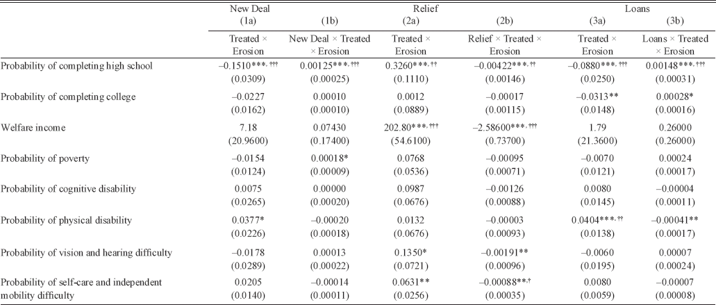
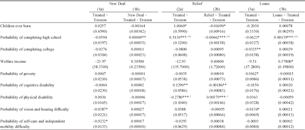
The results from these regressions are reported in Table 5 (for men) and Table 6 (for women). Public expenditure associated with the New Deal is found to ameliorate the adverse effects of Dust Bowl exposure in large and statistically significant ways. Relief spending in particular appears to mitigate the damage caused by Dust Bowl exposure: a one standard deviation increase in per capita relief spending reduces exposed men's welfare income by $60.13, and lowers the probability of work disability, vision and hearing disability, and self-care and independent living disability by 0.89, 4.49, and 2.05 percentage points, respectively. Per capita loans similarly ameliorate adverse impacts on male college completion and female work disability, albeit to a smaller degree: a one standard deviation increase in per capita loans is associated with a 0.66 percentage point greater chance of completing college, and the same increase in spending contributes to 0.52 percentage point lower rates of work disability amongst exposed women.
Broader New Deal expenditures, meanwhile, are associated with higher probabilities of high school completion among both exposed men (5.93 percentage points for a one standard deviation increase in spending) and exposed women (3.26 percentage points). Given that loans and broader New Deal spending are associated with higher probabilities of high school completion amongst the exposed, but the subset of New Deal spending focused on direct relief has the opposite effect, perhaps spending was most effective in improving secondary schooling outcomes where it was targeted at agricultural recovery and infrastructural investment. Clearly, state spending aimed at Depression and Dust Bowl recovery appears to have been effective in compensating for early-life insults and diminishing the worst Dust Bowl impacts on human capital, in particular those on disability and schooling. These results are consistent with some recent studies in modern developing countries, in which positive shocks to income have been shown to partially or even fully mitigate early-life deprivation (Gunnsteinsson, Adhvaryu, Christian, et al. Reference Gunnsteinsson, Adhvaryu and Christian2016; Adhvaryu, Molina, Nyshadham, et al. Reference Adhvaryu, Molina and Nyshadham2016). Importantly, relative to these comparatively short-run studies, I show that the effects of childhood remediation efforts can persist well into adulthood.
ROBUSTNESS
The results discussed thus far refer to coefficients that are statistically significant at the standard levels. However, many results, particularly those for college completion and disability, also survive the much stricter standards imposed by the Bonferroni correction for multiple comparisons.Footnote 22 Specifications including controls for age (to account for life cycle effects) and veteran status (to account for possible G.I. Bill benefit effects on postsecondary education and income/wealth) produce similar results to those in the baseline (not reported). Results are also robust to the removal of trends,Footnote 23 controls for place of residence and birth-residence migration paths,Footnote 24 alternate approaches to the standard errors,Footnote 25 alternate definitions of treated cohorts,Footnote 26 and alternate definitions of Dust Bowl severity (not reported). Clearly, the Dust Bowl was a meaningful shock that severely influenced the human capital and later-life welfare of those exposed.
Nevertheless, there are four major phenomena that could be said to have confounded effects that I attribute here to Dust Bowl exposure: the Great Depression, which could have affected childhood incomes independently of the Dust Bowl; migration from the Great Plains to the West, which could have affected duration of treatment and sample selection; and selection into the sample (fertility) or out of the sample (mortality). In this section, I provide evidence to suggest that these issues are unlikely to undermine my analysis and findings.Footnote 27
The Great Depression
First, the difference-in-differences approach is designed to test the effect of differences in the severity of Dust Bowl exposure even within cohorts in which all individuals were exposed to the Depression. Thus, as long as Depression severity is not systematically correlated with erosion (which does not appear to be the case), β 1 isolates the treatment effect of the Dust Bowl above and beyond the effects of the Great Depression.Footnote 28
Second, I control for several fixed effects and trends that account for variation beyond that due to the Dust Bowl. These include birth-year fixed effects, which control for nationwide macroeconomic shocks; birth-state fixed effects, which take into account a state's level of economic development; and state trends, which capture trends in state economic performance and public spending over time. Only if the Depression's effects varied dramatically within a state (for instance, spatially or demographically) might the latter two controls be insufficient to approximate the Depression's effect on individuals.Footnote 29 While controls for an individual's actual household income in childhood would be ideal, these figures are not available in the census data used here.
Lastly, in the absence of information on actual childhood household circumstances, I control for state-level childhood income per capita, meant to proxy for Great Depression effects (Fishback and Thomasson Reference Fishback and Thomasson2014).Footnote 30 Although, consistent with Fishback and Thomasson (Reference Fishback and Thomasson2014), childhood income has an intuitive and significant impact on outcomes such as disability, results on Dust Bowl exposure are robust to the inclusion of these controls (reported in Section 3 of the Online Appendix), which include real state per capita personal income in the birth year, in the year before birth, and averaged over childhood (ages –1 to 12). These results suggest that the Dust Bowl had adverse effects above and beyond those due to the Depression; indeed, it is likely that the Dust Bowl, and not just macroeconomic shocks, contributed to the low incomes experienced in this period in the Great Plains.
Migration
First, since migration status during childhood is unknown, equation (1) proceeds as an intent-to-treat analysis, meaning that the adverse effects estimated here are likely a lower bound on the true treatment effects of the Dust Bowl. Indeed, regressions disaggregating adult outcomes by (eventual) migrant status indicate that migrants had wellbeing outcomes similar to or better than non-migrants. This could be because Dust Bowl exposure was cut short by childhood out-migration, because the destination state offered better conditions to remediate early-life insults, or because migrants were positively selected on health or other related characteristics. In the first two cases, my analysis would, by conflating plausible migrants and non-migrants, actually understate the adverse effects experienced by exposed non-migrants (methods and results reported in Section 3 of the Online Appendix). If, however, the apparent better outcomes of migrants are exclusively a function of positive selection, then the Dust Bowl effects estimated here are neither under- nor over-estimates. I find little evidence of selection into migration when looking for socioeconomic-status gradients in the probability of migration during childhood (see Table A4). Although the data do not allow me to fully rule out selection into post-childhood migration, the baseline results are unchanged after adding controls for the state of adult residence and the birth-state-residence-state migration path. Finally, I find that childhood Dust Bowl severity has no significant effect on eventual migration status as an adult (see Section 3 of the Online Appendix).
Second, migration is unlikely to have affected childhood treatment. Even individuals migrating as children are unlikely to have escaped the phase in which I find the strongest adverse impacts of exposure: the –1 to 0 age band, a narrow and vulnerable timeframe in a child's life. This, added to the fact that interstate migration rates were actually “unusually” low during the 1930s (Rosenbloom and Sundstrom Reference Rosenbloom, Sundstrom, Wolcott and Hanes2004; Long and Siu Reference Long and Siu2016), suggests that migration during the treatment window is unlikely to influence exposure measures.
Third, I find little evidence of migrant selectivity. Neither Dust Bowl severity nor measures of household income and socioeconomic status, conditional on Dust Bowl treatment, are significant in determining the likelihood of migration in childhood (methods and results reported in Sections 1 and 3 of the Online Appendix). The only significant difference is found in Dust Bowl-exposed children from farm households, who were if anything less likely to have migrated before age 12 than the non-farm exposed, consistent with Jason Long and Henry E. Siu (Reference Long and Siu2016), who find that farmers were the least likely to have moved during the Dust Bowl. Secondary literature, too, suggests an ambiguous (or even non-existent) relationship between migrant status and individual/household characteristics, such as wealth, which one might expect to affect both treatment and the response to the shock (Lord Reference Lord1938; Wallace Reference Wallace1938; Worster Reference Worster1979; Nealand Reference Nealand2008; Burns, Duncan, and Dunfey Reference Burns, Duncan and Dunfey2012; Long and Siu Reference Long and Siu2016). Together, these findings suggest no systematic difference in migrant and non-migrant characteristics in this setting.
Fertility Selection
Work on crisis events such as famine and macroeconomic busts indicates that often in such periods, only those who can afford to provide for children will choose to continue bearing them (Dehejia and Lleras-Muney Reference Dehejia and Lleras-Muney2004; Ó Gráda Reference Ó Gráda2011). If such a phenomenon were at play during the Dust Bowl, I would expect that the individuals most resilient to and best able to compensate for the shock would disproportionately enter my sample, while many of the most vulnerable would never been born at all. This would tend to understate the adverse effects of the shock. Similarly, any involuntary reductions in fertility amongst Dust Bowl mothers (for instance, due to malnutrition- or stress-related amenorrhea) would also raise the average health status of the Dust Bowl cohort in ways that would lead me to underestimate the event's damage to later-life human capital (Ladurie Reference Ladurie1969).
I test for such fertility selection into my sample and find no statistically significant differences in fertility in response to the Dust Bowl by maternal socioeconomic status (methods and results reported in Sections 1 and 3 of the Online Appendix). Analysis of vital statistics shows that the timing and severity of erosion did not drive change in birth rates: indeed, states experienced no significant change in birth rates during the Dust Bowl period, consistent with Cutler, Miller, and Norton (Reference Cutler, Miller and Norton2007) and Fishback, Haines, and Kantor (Reference Fishback, Haines and Kantor2007). As a further check, regressions inferring Dust Bowl-era fertility adjustments from 1920–1950 Census cohort size in single-year age bands indicate no significant effect of childhood exposure to the Dust Bowl on cohort size (not reported).Footnote 31
Mortality Selection
Given that the individuals in the Dust Bowl cohort are aged anywhere from 39–82 by the time I observe them as adults in 1980–2000, survivorship bias may be a concern. That is, many of the individuals in poorest health as a result of Dust Bowl exposure may have died before being observed as adults, a “culling” effect that would bias the wellbeing of individuals in my sample upwards. If such an effect existed, my results would underestimate the true adverse effects of the Dust Bowl on health.
I find no significant change by Dust Bowl exposure in yearly state-level stillbirth rates and infant mortality rates (reported in Section 3 of the Online Appendix). Similarly, I test for whether the Dust Bowl cohort had significantly higher mortality rates than the unexposed at any stage in their life-course, up to and including my observation period. I find no significant difference in mortality rates, except in the 5–14 and 55–64 age bins, during which males in the Dust Bowl cohort experienced marginally lower mortality rates than their unexposed counterparts (methods and results reported in Sections 1 and 3 of the Online Appendix). These findings indicate that mortality selection and survivorship bias are unlikely to influence my results.
DISCUSSION
Taken as a whole, the results presented in this study not only suggest that the Dust Bowl had permanent consequences for health, but they also hint at when and how certain capabilities are developed. In this way, they shed light on the technology of human capital formation. For instance, the finding that health outcomes like disability are determined within the first year of life is reasonably intuitive, given that the fetal programming literature suggests that earlier developmental stages tend to disproportionately influence many health outcomes. However, it is striking that this early-life development pathway would also be responsible for outcomes like college completion and poverty, which one might expect to be associated with deficits in schooling and labor-market preparation resulting from shocks at school-going age. Indeed, given that high school completion rates rose amongst the exposed, why did not college completion rise as well, and poverty levels fall with this acquisition of education? Why does college completion behave like a health outcome? The answer might be that cognitive and physical impairments accrued in utero as a result of maternal poverty and ill-health influenced individuals' ability to enter and complete college, to hold down jobs, and to earn income as adults. That these impairments were not fully remediated by adulthood is consistent with dynamic models of capability formation, such as that in James Heckman (Reference Heckman2007), in which investments made further in time from a shock are less productive.Footnote 32
For contrast, increases in high school completion among the exposed (a notable exception to the infant exposure pattern more generally observed) suggest that secondary schooling outcomes may depend less on innate ability than on access to opportunity and questions of time use. As discussed briefly with respect to the results using the change in farm value, these increases in high school completion rates are substantial: for instance, men exposed between the ages of 7 and 12 see a 3.42 to 3.61 percentage point greater chance of finishing high school; for women, the figures are even higher, ranging from an extraordinary 4.89 to 6.39 percentage point increase. An analysis of the short-term impact of the Dust Bowl on school attendance corroborates this finding: 1940 teenagers born in more highly eroded states and counties were statistically significantly likelier to be attending school than their counterparts in 1930 (see Online Appendix and Tables A9–10 for more). Although the idea that a shock at schooling age would affect schooling is intuitive, finding positive outcomes on schooling may appear less intuitive at first glance. Here, the devastation of farming livelihoods may have played a role.
In particular, these findings suggest a tradeoff between secondary schooling and child labor in agriculture. Prior to the Dust Bowl's destruction of farms, child farm labor was prevalent. Robert Whaples (Reference Whaples2005) shows that in 1930, 74.5 percent of boys and 61.5 percent of girls aged 10–15 were employed in agriculture, and Karen Clay, Jeff Lingwall, and Melvin Stephens, Jr. (Reference Clay, Lingwall and Stephens2012) indicate that child labor was extensive even in the face of compulsory schooling laws, which were not strictly enforced. Laws restricting child labor, such as the 1938 Fair Labor Standards Act, contained many exemptions for child labor in agriculture, especially on family farms (U.S. Department of Labor Reference Department of Labor2007, Reference Department of Labor2013). Thus, the collapse of agriculture in the Great Plains may have reduced opportunities for child labor. Child labor and schooling have been shown to be closely related (McNay, Humphries, and Klasen Reference McNay, Humphries and Klasen2005; Bhalotra Reference Bhalotra2007; Clay, Lingwall, and Stephens, Jr. Reference Clay, Lingwall and Stephens2012; Baker Reference Baker2015). For instance, in present-day India, Sonia Bhalotra (Reference Bhalotra2007) finds that lowering the opportunity cost of schooling through cash transfers meant to offset the child's wages is essential to reducing child labor and increasing schooling. Poverty may have remained an issue for Dust Bowl households, but for them the lack of opportunities for labor in agriculture may have caused a drop in the opportunity cost of schooling. Indeed, Kirsty McNay, Jane Humphries, and Stephen Klasen (Reference McNay, Humphries and Klasen2005) find this phenomenon at play where higher rates of girls' schooling in nineteenth-century Britain are found in regions where opportunities for girls' employment were few. Richard Baker (Reference Baker2015) finds a similar effect in the twentieth-century U.S. South, where the boll weevil, a cotton pest, raised the school enrollment of black children, who were unusually active in agricultural work.
Together, the timing of the surge and the fact that farm population-weighting raises the magnitude of the Dust Bowl's high school completion effect suggest that a reduction in the need for child labor in agriculture following the destruction of farms may have lowered the opportunity cost of secondary schooling for school-age (i.e., working-age) children who now had no more profitable way to spend their time. Of course, increased high school completion may also reflect increased public spending—for instance, on school-building—as a response to the disaster. Most importantly to our understanding of human capital formation, despite both being educational outcomes, the fact that high school and college completion are associated with exposure in very different developmental stages suggests that these outcomes may in fact have very different inputs and production processes. For instance, childhood time allocation concerns appear to be important to pre-tertiary school attendance decisions (Moehling Reference Moehling1999; McNay, Humphries, and Klasen Reference McNay, Humphries and Klasen2005; Clay, Lingwall, and Stephens, Jr. Reference Clay, Lingwall and Stephens2012; Baker Reference Baker2015), while intellectual capability appears to be crucial to college completion (Heckman Reference Heckman2007). While for present-day households, credit constraints have been found less important than child ability in determining college enrollment (Heckman Reference Heckman2007), it should be noted that the same low incomes that may have played a role in producing poor college outcomes through fetal malnutrition, and thus, cognitive impairments in utero, may also have produced poor college outcomes through constraints on a Dust Bowl-stricken household's ability to afford college.
The results also shed light on the recovery process. Specifically, they show that public spending through New Deal and related programs helped mitigate the Dust Bowl's adverse effects. Thus, these findings provide striking evidence of the capacity for remediation through compensatory investments. Furthermore, they suggest that the New Deal was especially long-reaching through its beneficial effects on individuals' life-course wellbeing. Although these results indicate that some measure of recovery may in fact be possible, the findings that recovery is incomplete, and that those exposed in earlier stages suffer worse outcomes than those struck later on in life, nevertheless suggest that investments in human capital cannot be perfectly substituted across periods in a child's development. Thus, as Heckman (Reference Heckman2007) and Douglas Almond and Janet Currie (Reference Almond, Currie, Ashenfelter and Card2011a) discuss, the assumption that investments have linear effects across childhood is likely an unrealistic one.
CONCLUSION
Through this analysis, I use variation in childhood Dust Bowl exposure to show that this natural disaster had meaningful long-term human capital costs for those exposed as children. For women, fertility and college completion rates fell, while poverty rates rose. For men, poverty rates, welfare receipts, and disability rates rose. Notably, these adverse effects were most severe for those exposed in utero and in early childhood, implicating an indirect health pathway—that is, poor prenatal nutrition and health, and through it, disrupted capability development—in the production of these impacts.
For all, but especially for women, high school completion rates rose. In contrast to the sensitive periods implicated in the bulk of the outcomes studied here, the impact on secondary schooling was greatest on children who experienced the Dust Bowl in late childhood and early adolescence, when the tradeoff between child farm labor and formal schooling likely dictated time use. In these outcomes (unlike in college completion, which suffered as a result of the Dust Bowl), family income and student cognitive ability were unlikely to be barriers to entry. Results like these offer suggestive and policy-relevant evidence on when and how different capabilities are formed—for example, substantiating the hypothesis that college-readiness may be strongly determined in utero and in early childhood, and suggesting that postsecondary educational interventions should be targeted accordingly. Finally, New Deal-related expenditure is found to have attenuated the Dust Bowl's adverse effects, demonstrating the capacity for remediation even where private investment in recovery may have been constrained in light of large income shocks.
As intent-to-treat rather than treatment-on-the-treated estimates, my results represent the lower bounds on the actual later-life effects of childhood Dust Bowl exposure. This intent-to-treat design stems from a limitation in census data: the absence of information on individuals' circumstances as children. Although adult outcomes cannot be linked to childhood erosion below the state level, making it difficult to accurately gauge an individual's actual Dust Bowl exposure, true erosion exposure may not be as strongly tied to birth county erosion as expected. Accordingly, the state-level construction of erosion exposure may actually yield two advantages over county-level construction. First, a less localized measure reflects the reality of the considerable intra-state, inter-county migration documented within the Dust Bowl region (Long and Siu Reference Long and Siu2016), and second, a state-level measure is likelier to capture downwind externalities (Hansen and Libecap Reference Hansen and Libecap2004). Nevertheless, I do take steps to account for the likely level, timing, and duration of exposure. First, I weight erosion by county population, allowing for a more realistic measure of the severity of human exposure within a state. Second, I disaggregate exposure by developmental stage. Finally, since these data do not allow for analysis of the effects of differences in parental or household characteristics in childhood, I include state-level proxies for childhood economic circumstances.
These results represent an important contribution to our understanding of the Dust Bowl's impacts; namely, they show quantitatively that exposed children suffered long-term and meaningful damage to health and human capital. Perhaps more important, however, is the finding that such harm can be overcome through timely and substantial policy intervention.