


1 Introduction
Turbulent flows in the natural environment often evolve under the influences of ambient current shear and stable density stratification. For example, stably stratified shear layers have been observed in the oceans and in the atmosphere (Woods Reference Woods1968; De Silva et al. Reference De Silva, Fernando, Eaton and Hebert1996), where the shear can produce turbulence that can promote large rates of mixing. These observations in field experiments have led many researchers to study stably stratified shear layers with theories, laboratory experiments and numerical simulations, as summarized in review articles (Thorpe Reference Thorpe1973b ; Fernando Reference Fernando1991; Peltier & Caulfield Reference Peltier and Caulfield2003).
Laboratory experiments and numerical simulations often consider a stably stratified shear layer where shear and stratification are localized in a thin layer, across which both mean velocity and density vary in the vertical direction (Thorpe Reference Thorpe1973a ; Smyth & Moum Reference Smyth and Moum2000b ; Brucker & Sarkar Reference Brucker and Sarkar2007; Mashayek & Peltier Reference Mashayek and Peltier2012a ,Reference Mashayek and Peltier b ). Many studies on stratified shear layers have been devoted to understanding instabilities and transition to turbulence. When the initial bulk Richardson number is lower than a critical value, turbulence is generated by the Kelvin–Helmholtz instability and causes mixing of the fluids of different densities (Strang & Fernando Reference Strang and Fernando2001). The development of the stably stratified shear layer results in a density profile that is consistent with some observations in the oceans (Moum Reference Moum1996; Smyth & Moum Reference Smyth and Moum2000b ). The generated turbulence ultimately begins to rapidly decay with time under the influence of stable stratification. Smyth & Moum (Reference Smyth and Moum2000b ) have also investigated the evolution of various length scales for a wide range of Reynolds number, Richardson number and Prandtl number. Mashayek, Caulfield & Peltier (Reference Mashayek, Caulfield and Peltier2017) have shown the relation between the characteristics of turbulent mixing and various length scales and parameters of the stably stratified shear layers for much larger Reynolds number than in Smyth & Moum (Reference Smyth and Moum2000b ).
Turbulence is often studied in terms of its coherent structures. These structures are typified by their length scales and characteristic coherent patterns, which are extended in space and time (Pope Reference Pope2000). It is often sought to understand and explain a flow field in terms of a small number of these structures. Various structures have been identified in wall-bounded shear flows, such as low-speed streaks, outward ejections of low-speed fluid and hairpin-shaped vortical structures (Robinson Reference Robinson1991). These structures have been extensively studied using both numerical simulations and experiments (e.g. Head & Bandyopadhyay Reference Head and Bandyopadhyay1981; Zhou et al. Reference Zhou, Adrian, Balachandar and Kendall1999; Adrian, Meinhart & Tomkins Reference Adrian, Meinhart and Tomkins2000; Schoppa & Hussain Reference Schoppa and Hussain2002; Carlier & Stanislas Reference Carlier and Stanislas2005; Wu & Moin Reference Wu and Moin2009). Previous studies have also found highly elongated flow structures, with both positive and negative streamwise velocity fluctuations, which are termed ‘superstructures’ in turbulent boundary layers (Hutchins & Marusic Reference Hutchins and Marusic2007) and ‘very large-scale motions’ in turbulent pipe flows (Kim & Adrian Reference Kim and Adrian1999). These long flow structures are shown to be important, with significant turbulent kinetic energy (Hutchins & Marusic Reference Hutchins and Marusic2007), and their influence on small-scale features near a wall is noteworthy, as reported by Mathis, Hutchins & Marusic (Reference Mathis, Hutchins and Marusic2009). More studies on these very long structures in wall turbulence can be found, for example, in Monty et al. (Reference Monty, Stewart, Williams and Chong2007, Reference Monty, Hutchins, Ng, Marusic and Chong2009), Hellström, Sinha & Smits (Reference Hellström, Sinha and Smits2011), Wu, Baltzer & Adrian (Reference Wu, Baltzer and Adrian2012), Lee & Sung (Reference Lee and Sung2013).
The present study investigates the flow structures in a stably stratified shear layer with localized shear and stratification. Direct numerical simulations (DNS) in a very large computational domain allow us to explore large-scale structures as well as smaller-scale ones in a turbulent stably stratified shear layer. Our DNS confirms the existence of hairpin-shaped vortices and highly elongated structures with positive and negative streamwise velocity fluctuations, both of which are similar to the structures found in wall-bounded shear flows. The flow associated with the hairpin vortices is shown to contribute the vertical transfer of momentum and density even when the Kolmogorov scale is of the same order as the Ozmidov scale.
In § 2 we discuss the details of our simulation methodology, and some of the important dimensional and non-dimensional parameters in the problem. In § 3 we then present in detail our results, and in § 4 we summarize our conclusions from this study.
2 Direct numerical simulations of stably stratified shear layer
We consider temporally evolving, stably stratified shear layers with localized shear and stratification (Smyth & Moum Reference Smyth and Moum2000b
), which have also been studied with different parameters by DNS in our previous papers; details of our results and methodology can be found in Watanabe, Riley & Nagata (Reference Watanabe, Riley and Nagata2016, Reference Watanabe, Riley and Nagata2017). The streamwise, spanwise and vertical directions are represented by
 $x$
,
 $y$
and
 $z$
, respectively, and the corresponding components of the velocity vector are
 $u$
,
 $v$
and
 $w$
. The density field is expressed as
 $\unicode[STIX]{x1D70C}_{a}+\unicode[STIX]{x1D70C}(x,y,z;t)$
, with
 $\unicode[STIX]{x1D70C}_{a}$
a constant reference value, and the deviation from
 $\unicode[STIX]{x1D70C}_{a}$
denoted by
 $\unicode[STIX]{x1D70C}$
. The governing equations are the Navier–Stokes equations with the Boussinesq approximation, written as
 $$\begin{eqnarray}\displaystyle & \displaystyle \frac{\unicode[STIX]{x2202}u_{j}}{\unicode[STIX]{x2202}x_{j}}=0, & \displaystyle\end{eqnarray}$$
 $$\begin{eqnarray}\displaystyle & \displaystyle \frac{\unicode[STIX]{x2202}u_{i}}{\unicode[STIX]{x2202}t}+\frac{\unicode[STIX]{x2202}u_{i}u_{j}}{\unicode[STIX]{x2202}x_{j}}=-\frac{1}{\unicode[STIX]{x1D70C}_{a}}\frac{\unicode[STIX]{x2202}p}{\unicode[STIX]{x2202}x_{i}}+\unicode[STIX]{x1D708}\frac{\unicode[STIX]{x2202}^{2}u_{i}}{\unicode[STIX]{x2202}x_{j}\unicode[STIX]{x2202}x_{j}}-g\frac{\unicode[STIX]{x1D70C}}{\unicode[STIX]{x1D70C}_{a}}\unicode[STIX]{x1D6FF}_{i3}, & \displaystyle\end{eqnarray}$$
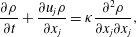 $$\begin{eqnarray}\displaystyle & \displaystyle \frac{\unicode[STIX]{x2202}\unicode[STIX]{x1D70C}}{\unicode[STIX]{x2202}t}+\frac{\unicode[STIX]{x2202}u_{j}\unicode[STIX]{x1D70C}}{\unicode[STIX]{x2202}x_{j}}=\unicode[STIX]{x1D705}\frac{\unicode[STIX]{x2202}^{2}\unicode[STIX]{x1D70C}}{\unicode[STIX]{x2202}x_{j}\unicode[STIX]{x2202}x_{j}}, & \displaystyle\end{eqnarray}$$
where the integers
 $i,j=1$
, 2 and 3 denote the
 $x$
,
 $y$
and
 $z$
directions,
 $\unicode[STIX]{x1D708}$
is the kinematic viscosity,
 $\unicode[STIX]{x1D705}$
is the diffusivity coefficient for density and
 $g$
is the gravitational acceleration. The gravitational force appears in the momentum equation in the
 $z$
direction.
The flow develops with time in a computational domain that is taken to be periodic in both horizontal directions. The initial mean streamwise velocity is given by
 $\langle u\rangle =0.5U_{0}\tanh (2z/h_{0})$
, where
 $\langle \cdot \rangle$
is an averaged value taken on a homogeneous plane,
 $U_{0}$
is the velocity difference across the shear layer and
 $h_{0}$
is the initial shear layer thickness. The initial mean velocity is zero for
 $v$
and
 $w$
. The initial velocity field is obtained by superimposing velocity fluctuations onto the mean velocity as
 $u=\langle u\rangle +u^{\prime }$
,
 $v=v^{\prime }$
and
 $w=w^{\prime }$
, where fluctuations
 $u^{\prime }$
,
 $v^{\prime }$
and
 $w^{\prime }$
are obtained by a diffusion process that converts random noise to spatially correlated fluctuations (Kempf, Klein & Janicka Reference Kempf, Klein and Janicka2005). The initial density field is given as
 $\unicode[STIX]{x1D70C}=-0.5\unicode[STIX]{x1D70C}_{0}\tanh (2z/h_{0})$
without any density perturbation, where
 $\unicode[STIX]{x1D70C}_{0}$
is the density difference across the stably stratified shear layer.
The flow is characterized by three non-dimensional parameters: the Reynolds number
 $Re=U_{0}h_{0}/\unicode[STIX]{x1D708}$
, the Prandtl number
 $Pr=\unicode[STIX]{x1D708}/\unicode[STIX]{x1D705}$
and the bulk Richardson number
 $Ri=g\unicode[STIX]{x1D70C}_{0}h_{0}/\unicode[STIX]{x1D70C}_{a}U_{0}^{2}$
. The Prandtl number affects the ratio between the smallest length scales of velocity and density fields, where this ratio is expected to be
 $O(1)$
in the case of
 $Pr=1$
. For simplicity, all the simulations are conducted with
 $Pr=1$
for investigating dependence of the flow on
 $Re$
and
 $Ri$
. Because the smallest length scale of density fluctuations decreases as
 $Pr$
increases, larger
 $Pr$
requires smaller grid spacing in the DNS, which increases the computational cost. The DNS are conducted in a computational domain with the size of
 $(L_{x}\times L_{y}\times L_{z})=(448h_{0},84h_{0},140h_{0})$
, which is discretized by (
 $N_{x}\times N_{y}\times N_{z}$
) grid points. This computational domain is much larger than the roller vortices arising from the Kelvin–Helmholtz instability. Previous numerical simulations of stratified shear layers sometimes used a computational domain whose streamwise extent is comparable to the roller vortices, because these studies mainly investigated the instabilities and transition (Smyth & Moum Reference Smyth and Moum2000b
; Mashayek & Peltier Reference Mashayek and Peltier2012a
). A significantly larger domain than most in previous numerical simulations is used in this study since its purpose is to investigate large-scale structures that appear after the transition. Uniform grid spacing is used in both horizontal directions, while the grid is stretched in the vertical direction near the vertical boundaries using a mapping function employed by Watanabe et al. (Reference Watanabe, Riley, Nagata, Onishi and Matsuda2018), while a finer grid is employed near the shear layer. The grid size near the centre line is set to be the same for all three directions, i.e.
 $\unicode[STIX]{x1D6E5}_{x}=\unicode[STIX]{x1D6E5}_{y}=\unicode[STIX]{x1D6E5}_{z}$
. Periodic boundary conditions are applied in the two horizontal directions, while the free-slip boundary conditions are applied to the velocity, and zero-flux conditions to the density, at the top and bottom of the computational domain.
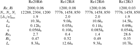
Parameters for the DNS of stably stratified shear layers. The table also presents values for
 $\unicode[STIX]{x1D6FF}_{u}$
,
 $L_{O}$
,
 $\unicode[STIX]{x1D702}$
,
 $Re_{b}$
,
 $Ri_{g}$
and
 $L_{\unicode[STIX]{x1D700}}$
at
 $z=0$
and
 $t=320t_{r}$
.
The DNS code is the same as the one used for stratified shear layers in Watanabe et al. (Reference Watanabe, Riley and Nagata2016, Reference Watanabe, Riley and Nagata2017, Reference Watanabe, Riley, Nagata, Onishi and Matsuda2018). The code is based on the fractional step method. Second- and fourth-order fully conservative central difference schemes are used in the vertical and horizontal directions, respectively, while a third-order Runge–Kutta method is used for temporal advancement. The Poisson equation for pressure is solved using the biconjugate gradient stabilized (Bi-CGSTAB) method.
Four simulations are carried out with parameters summarized in table 1. Most of the results presented are for case Re20Ri6, while other simulations are used for examining the effects of
 $Re$
and
 $Ri$
. Averages taken on a horizontal plane
 $\langle \cdot \rangle$
are obtained as functions of the vertical location and time. In this paper, a fluctuation of variable
 $f$
from the average
 $\langle f\rangle$
is denoted as
 $f^{\prime }=f-\langle f\rangle$
.
Important length scales and non-dimensional numbers used in the discussion are defined here. The mean velocity
 $\langle u\rangle$
increases in the
 $z$
direction from
 $-0.5U_{0}$
to
 $0.5U_{0}$
across the shear layer. Therefore, the shear layer thickness
 $\unicode[STIX]{x1D6FF}_{u}$
can be estimated as the distance between vertical locations of
 $\langle u\rangle =0.49U_{0}$
and
 $\langle u\rangle =-0.49U_{0}$
. An integral length scale of the flow is defined as
 $$\begin{eqnarray}\displaystyle L_{\unicode[STIX]{x1D700}}=q^{3}/\unicode[STIX]{x1D700}, & & \displaystyle\end{eqnarray}$$
where
 $q^{2}=\langle u_{i}^{\prime }u_{i}^{\prime }\rangle$
is twice the turbulent kinetic energy,
 $\unicode[STIX]{x1D700}=2\unicode[STIX]{x1D708}\langle \unicode[STIX]{x1D634}_{ij}^{\prime }\unicode[STIX]{x1D634}_{ij}^{\prime }\rangle$
is the turbulent kinetic energy dissipation rate and
 $\unicode[STIX]{x1D634}_{ij}^{\prime }$
is the fluctuating rate-of-strain tensor. The mean vertical shear and the buoyancy frequency are defined as
 $S=\langle \unicode[STIX]{x2202}u/\unicode[STIX]{x2202}z\rangle$
and
 $N=\sqrt{-(g/\unicode[STIX]{x1D70C}_{a})\langle \unicode[STIX]{x2202}\unicode[STIX]{x1D70C}/\unicode[STIX]{x2202}z\rangle }$
, respectively. One of the important length scales in stably stratified turbulence is the Ozmidov scale, defined by
 $$\begin{eqnarray}\displaystyle L_{O}=\sqrt{\unicode[STIX]{x1D700}/N^{3}}. & & \displaystyle\end{eqnarray}$$
The Ozmidov scale is considered to be the smallest length scale that is affected by buoyancy, so that vertical motions at scales greater than the Ozmidov scale are strongly suppressed under stable stratification. On the other hand, the smallest length scale of turbulence is the Kolmogorov scale, defined by
 $$\begin{eqnarray}\displaystyle \unicode[STIX]{x1D702}=(\unicode[STIX]{x1D708}^{3}/\unicode[STIX]{x1D700})^{1/4}. & & \displaystyle\end{eqnarray}$$
In the present DNS, the Kolmogorov scale takes its smallest value at
 $t\approx 100t_{r}$
(
 $t_{r}=h_{0}/U_{0}$
), and then increases with time because of the decay of
 $\unicode[STIX]{x1D700}$
(Smyth & Moum Reference Smyth and Moum2000b
). The table shows the maximum values of
 $\unicode[STIX]{x1D6E5}_{x}/\unicode[STIX]{x1D702}$
on the centre line during the simulation. All simulations are performed with
 $\unicode[STIX]{x1D6E5}_{x}/\unicode[STIX]{x1D702}\leqslant 2.0$
, which is small enough for the central difference schemes used in the DNS to adequately capture the dissipation spectrum of these turbulent flows (Watanabe et al.
Reference Watanabe, Riley, Nagata, Onishi and Matsuda2018). The table also shows
 $\unicode[STIX]{x1D6FF}_{u}$
and centre line values of
 $L_{\unicode[STIX]{x1D700}}$
,
 $L_{O}$
and
 $\unicode[STIX]{x1D702}$
at
 $t=320t_{r}$
. The value of
 $\unicode[STIX]{x1D6FF}_{u}$
decreases as
 $Ri$
increases, although it only weakly depends on
 $Re$
for the
 $Ri$
and
 $Re$
considered in this study. The gradient Richardson number
 $Ri_{g}$
and buoyancy Reynolds number
 $Re_{b}$
are defined as
 $$\begin{eqnarray}\displaystyle & \displaystyle Ri_{g}=N^{2}/S^{2}, & \displaystyle\end{eqnarray}$$
 $$\begin{eqnarray}\displaystyle & \displaystyle Re_{b}=(L_{O}/\unicode[STIX]{x1D702})^{4/3}=\unicode[STIX]{x1D700}/\unicode[STIX]{x1D708}N^{2}. & \displaystyle\end{eqnarray}$$
As can be seen in its definition,
 $Re_{b}$
takes a large value when the Ozmidov scale is much greater than the Kolmogorov scale. In this case, there is a range of turbulent length scales for which direct influences of buoyancy are not significant. On the other hand,
 $Re_{b}=O(10^{0})$
results in suppression of turbulent motions at all scales because then
 $L_{O}\sim \unicode[STIX]{x1D702}$
, for which motions at the smallest turbulent length scale are also strongly influenced by buoyancy. Also
 $Re_{b}$
is used as a measure of intensity of turbulence in oceanography (Barry et al.
Reference Barry, Ivey, Winters and Imberger2001; Shih et al.
Reference Shih, Koseff, Ivey and Ferziger2005; de Lavergne et al.
Reference de Lavergne, Madec, Le Sommer, Nurser and Naveira Garabato2016). The table also shows the gradient Richardson number
 $Ri_{g}$
and buoyancy Reynolds number
 $Re_{b}$
at
 $t=320t_{r}$
on the centre line. The temporal evolutions of
 $\unicode[STIX]{x1D6FF}_{u}$
,
 $L_{O}$
,
 $\unicode[STIX]{x1D702}$
,
 $Ri_{g}$
and
 $Re_{b}$
are shown in the next section.
3 Results and discussions
3.1 Temporal evolution of stably stratified shear layer
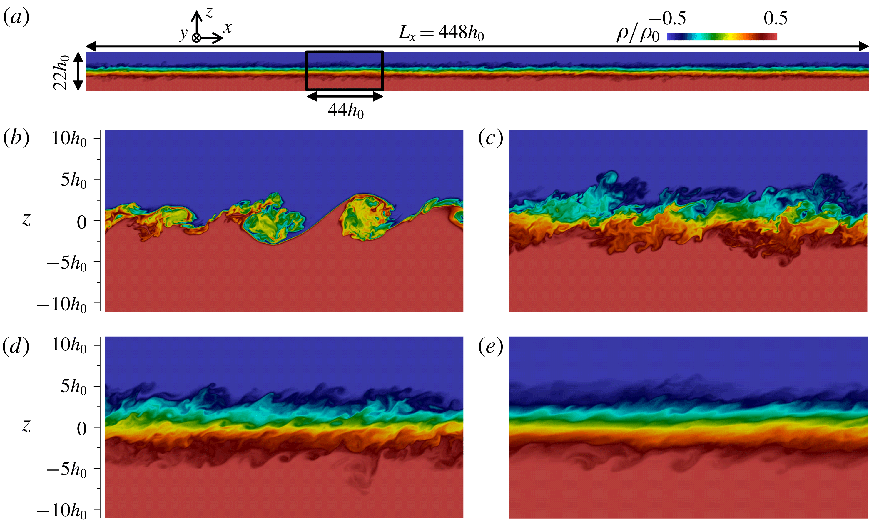
Figure 1(a) visualises the density field
 $\unicode[STIX]{x1D70C}$
on an
 $x$
–
 $z$
plane at
 $t/t_{r}=320$
for case Re20Ri6, while figure 1(b–e) show
 $\unicode[STIX]{x1D70C}$
at
 $t/t_{r}=80$
, 160, 240 and 320 in the box region shown in figure 1(a). It is seen that turbulence in the shear layer develops, due to Kelvin–Helmholtz instability, by
 $t/t_{r}=80$
. The roller vortices of the instability have already paired before
 $t/t_{r}=80$
. The streamwise length of the initial roller vortices before pairing, estimated from the density profile on an
 $x$
–
 $z$
plane, is about
 $2h_{0}$
-
 $4h_{0}$
at
 $t/t_{r}=40$
in all the DNS. The density field in figure 1(c) exhibits patterns associated with small scales of turbulence while density is more stratified in the shear layer at later time in figure 1(e).
From the DNS of a temporally evolving, stably stratified shear layer (Re20Ri6). (a) Density field at
 $t=320t_{r}$
in an
 $x$
–
 $z$
plane which includes the full length of the computational domain in the streamwise direction. Density field in the region marked by the box in (a) at (b)
 $t=80t_{r}$
, (c)
 $160t_{r}$
, (d)
 $240t_{r}$
and (e)
 $320t_{r}$
. The total extent of the computational domain in the vertical (
 $z$
) direction is not shown.
The evolution of statistics in a temporally evolving, stably stratified shear layer (Re20Ri6). (a) turbulent kinetic energy
 $k_{T}$
and density fluctuation variance
 $\langle {\unicode[STIX]{x1D70C}^{\prime }}^{2}\rangle$
, (b) Kolmogorov scale
 $\unicode[STIX]{x1D702}$
, Ozmidov scale
 $L_{O}$
and shear layer thickness
 $\unicode[STIX]{x1D6FF}_{u}$
, and (c) buoyancy Reynolds number
 $Re_{b}$
and gradient Richardson number
 $Ri_{g}$
.
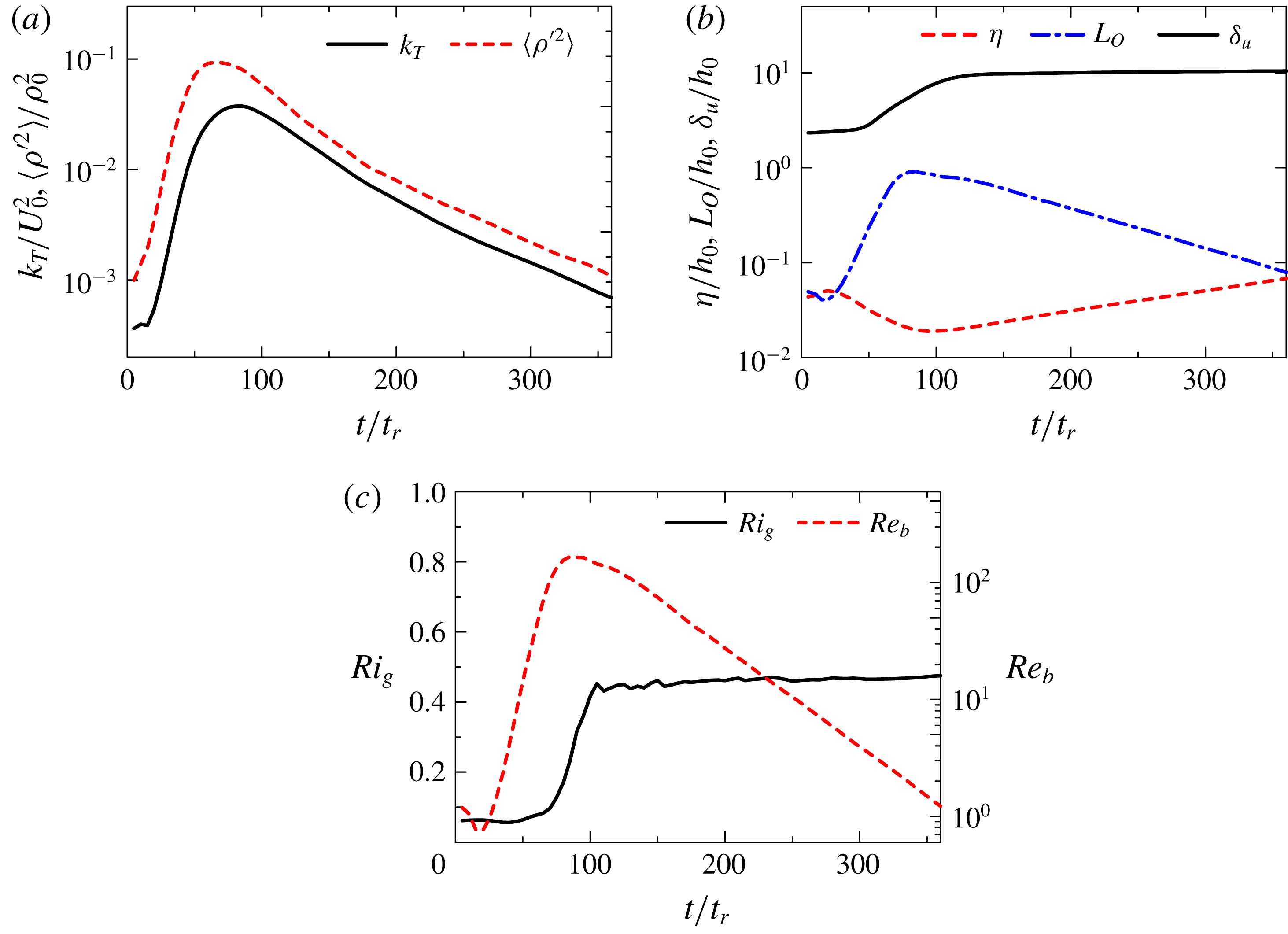
Figure 2 shows temporal evolutions of statistics in case Re20Ri6. Figure 2(a) plots density fluctuation variance
 $\langle {\unicode[STIX]{x1D70C}^{\prime }}^{2}\rangle$
and turbulent kinetic energy
 $k_{T}=\langle u_{i}^{\prime }u_{i}^{\prime }/2\rangle$
on the centre line, while figure 2(b) plots the shear layer thickness
 $\unicode[STIX]{x1D6FF}_{u}$
, Kolmogorov scale
 $\unicode[STIX]{x1D702}$
and Ozmidov scale
 $L_{O}$
on the centre line. As the turbulent shear layer grows from
 $t=0$
,
 $\langle {\unicode[STIX]{x1D70C}^{\prime }}^{2}\rangle$
,
 $k_{T}$
and
 $\unicode[STIX]{x1D6FF}_{u}$
initially increase with time. Then the shear layer stops growing as attested by the behaviour of
 $\unicode[STIX]{x1D6FF}_{u}$
for
 $t/t_{r}\geqslant 100$
, and the density and velocity fluctuations then decay rapidly with time. As these fluctuations decay, the Kolmogorov scale and Ozmidov scale increase and decrease, respectively, as also reported in previous DNS studies (Smyth & Moum Reference Smyth and Moum2000b
).
Figure 2(c) shows temporal evolutions of
 $Ri_{g}$
and
 $Re_{b}$
on the centre line for case Re20Ri6. Once the turbulent shear layer has developed,
 $Ri_{g}$
becomes almost independent of time, with the value of about
 $0.45$
. On the other hand,
 $Re_{b}$
ultimately decreases with time from
 $O(10^{2})$
to
 $O(10^{0})$
, implying that turbulent motions at very small scales also become directly affected by buoyancy, as the Ozmidov scale becomes as small as the Kolmogorov scale. Salehipour, Peltier & Mashayek (Reference Salehipour, Peltier and Mashayek2015) showed that the decay of
 $Re_{b}$
in late time is hardly affected by the Prandtl number for
 $1\leqslant Pr\leqslant 16$
in the stably stratified shear layers. Further details of stratified shear layer development can be found in previous studies (Smyth & Moum Reference Smyth and Moum2000b
; Brucker & Sarkar Reference Brucker and Sarkar2007; Watanabe et al.
Reference Watanabe, Riley and Nagata2016, Reference Watanabe, Riley and Nagata2017; Mashayek et al.
Reference Mashayek, Caulfield and Peltier2017).
The vertical profiles of (a) mean streamwise velocity
 $\langle u\rangle$
and density
 $\langle \unicode[STIX]{x1D70C}\rangle$
, (b) intermittency factor and (c) root mean square (r.m.s.) velocity fluctuations defined with average over the turbulent fluid
 $\langle \cdot \rangle _{T}$
or with conventional average for case Re20Ri6. (c) shows the results at
 $t=320t_{r}$
.
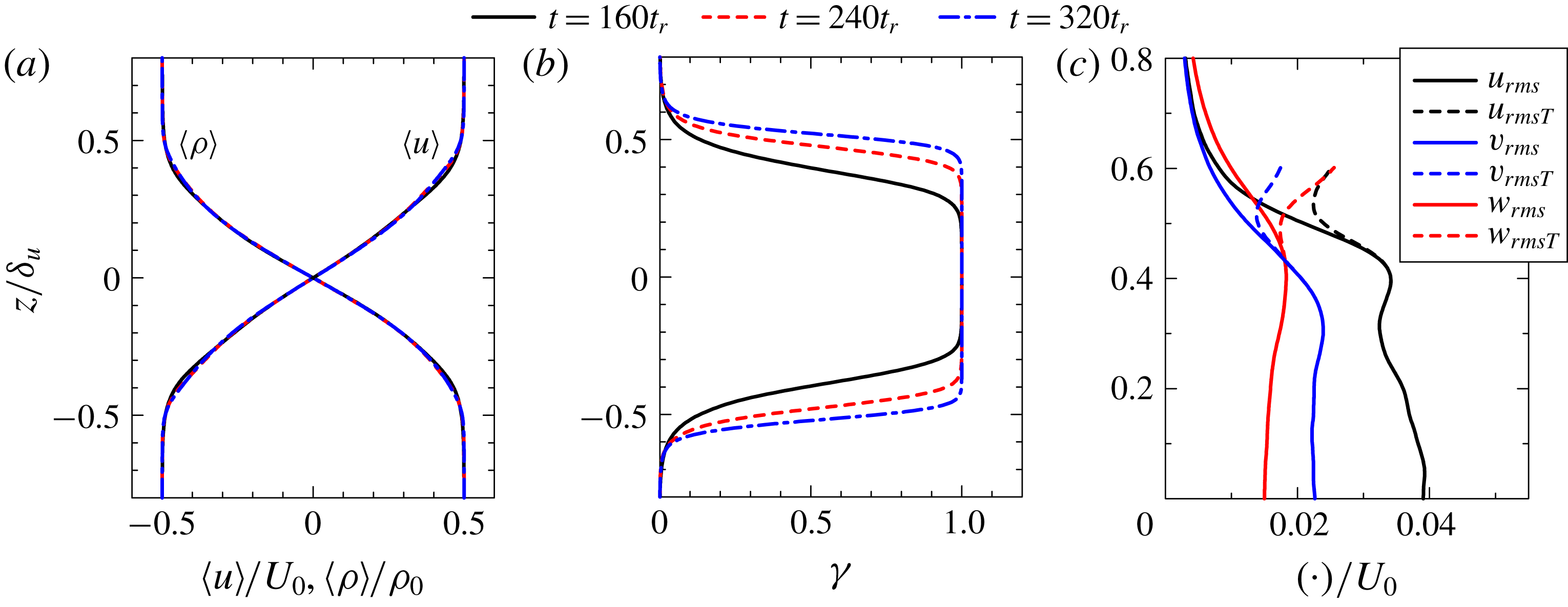
Figure 3(a) shows the vertical profiles of
 $\langle u\rangle$
and
 $\langle \unicode[STIX]{x1D70C}\rangle$
, where the vertical coordinate is normalized by the shear layer thickness
 $\unicode[STIX]{x1D6FF}_{u}$
. The normalized profiles of
 $\langle u\rangle$
and
 $\langle \unicode[STIX]{x1D70C}\rangle$
hardly change with time from
 $t=160t_{r}$
to
 $320t_{r}$
. Turbulent shear layers are known to be intermittent, and a flow can be turbulent or non-turbulent at a fixed location. Since turbulent structures are investigated in this study, it is important to show the spatial distribution of turbulent fluids in the stably stratified shear layer. Because a turbulent flow is characterized by its vorticity (Corrsin & Kistler Reference Corrsin and Kistler1955), the turbulent region in the stably stratified shear layer can be detected as the region with
 $|\unicode[STIX]{x1D74E}|\geqslant \unicode[STIX]{x1D714}_{th}$
, where
 $|\unicode[STIX]{x1D74E}|$
is the magnitude of the vorticity vector and
 $\unicode[STIX]{x1D714}_{th}$
is a suitably chosen threshold value (Watanabe et al.
Reference Watanabe, Riley and Nagata2016). The turbulent region also has higher kinetic energy dissipation rate than the non-turbulent region. The difference between turbulent and non-turbulent regions is clearer for vorticity magnitude (enstrophy) than kinetic energy dissipation rate in free shear flows (da Silva & Pereira Reference da Silva and Pereira2008). This is why the vorticity magnitude has been used for detecting the turbulent region in intermittent turbulent flows (da Silva et al.
Reference da Silva, Hunt, Eames and Westerweel2014). It should be noted that the regions outside of the shear layer have constant density values that do not support the propagation of internal gravity waves, unlike in turbulent shear layers developing in a stably stratified fluid (Watanabe et al.
Reference Watanabe, Riley, Nagata, Onishi and Matsuda2018). The threshold value
 $\unicode[STIX]{x1D714}_{th}$
is determined based on the mean vorticity magnitude on the centre line,
 $\langle |\unicode[STIX]{x1D74E}|\rangle _{C}$
, as
 $\unicode[STIX]{x1D714}_{th}=0.04\langle |\unicode[STIX]{x1D74E}|\rangle _{C}$
following our previous studies on turbulent/non-turbulent interfaces in stably stratified shear layers (Watanabe et al.
Reference Watanabe, Riley and Nagata2016, Reference Watanabe, Riley and Nagata2017). An intermittency function
 $I(x,y,z)$
is defined to be
 $I=1$
for a turbulent fluid and
 $I=0$
for a non-turbulent fluid (Pope Reference Pope2000). The intermittency factor
 $\unicode[STIX]{x1D6FE}$
, defined as the probability that the flow is turbulent, can be obtained by taking the average of
 $I$
as
 $\unicode[STIX]{x1D6FE}=\langle I\rangle$
. Figure 3(b) shows the vertical profile of
 $\unicode[STIX]{x1D6FE}$
at
 $t=160t_{r}$
,
 $240t_{r}$
and
 $320t_{r}$
for case Re20Ri6. The region near the centre line
 $z=0$
has
 $\unicode[STIX]{x1D6FE}=1$
, and the middle of the shear layer is always turbulent. At
 $t=160t_{r}$
,
 $\unicode[STIX]{x1D6FE}$
begins to decrease with
 $|z/\unicode[STIX]{x1D6FF}_{u}|$
for
 $|z/\unicode[STIX]{x1D6FF}_{u}|>0.2$
, as non-turbulent fluids appear in this region. At
 $t=240t_{r}$
and
 $320t_{r}$
,
 $\unicode[STIX]{x1D6FE}<1$
can be found for
 $|z/\unicode[STIX]{x1D6FF}_{u}|>0.4$
, and
 $\unicode[STIX]{x1D6FE}$
decreases with
 $|z/\unicode[STIX]{x1D6FF}_{u}|$
more sharply than at
 $t=160t_{r}$
. This confirms that the region where both turbulent and non-turbulent fluids coexist becomes narrower with time. This tendency is consistent with other observations that the turbulent/non-turbulent interface is flattened by the influence of stable stratification (Krug et al.
Reference Krug, Holzner, Lüthi, Wolf, Kinzelbach and Tsinober2015; Watanabe et al.
Reference Watanabe, Riley and Nagata2016, Reference Watanabe, Riley and Nagata2017). From its definition,
 $\unicode[STIX]{x1D6FE}=0$
implies that there are no turbulent motions at a certain height. Therefore, figure 3(b) also indicates that turbulent motions reach up to
 $|z/\unicode[STIX]{x1D6FF}_{u}|\approx 0.6{-}0.7$
. At
 $t=320t_{r}$
,
 $\unicode[STIX]{x1D6FE}$
is about
 $0.05$
at
 $|z/\unicode[STIX]{x1D6FF}_{u}|\approx 0.6$
, and the region of
 $|z/\unicode[STIX]{x1D6FF}_{u}|>0.6$
consists mostly of non-turbulent motions. Therefore, statistics related to turbulent structures are presented in the region of
 $|z/\unicode[STIX]{x1D6FF}_{u}|\leqslant 0.6$
in this paper.
The intermittency function
 $I$
can be used for defining averages taken for turbulent fluids as
 $\langle f\rangle _{T}=\langle fI\rangle /\langle I\rangle$
(Pope Reference Pope2000). Figure 3(c) shows the r.m.s. velocity fluctuations of the turbulent fluids,
 $u_{rmsT}=\sqrt{\langle u^{2}\rangle _{T}-\langle u\rangle _{T}^{2}}$
,
 $v_{rmsT}=\sqrt{\langle v^{2}\rangle _{T}-\langle v\rangle _{T}^{2}}$
and
 $w_{rmsT}=\sqrt{\langle w^{2}\rangle _{T}-\langle w\rangle _{T}^{2}}$
, in the upper side of the shear layer (
 $z\geqslant 0$
) at
 $t=320t_{r}$
. Here, the average for turbulent fluids is computed in the region with
 $\unicode[STIX]{x1D6FE}\geqslant 0.05$
. For comparison, the figure also shows the r.m.s. velocity fluctuations defined with the conventional average,
 $u_{rms}=\sqrt{\langle u^{2}\rangle -\langle u\rangle ^{2}}$
,
 $v_{rms}=\sqrt{\langle v^{2}\rangle -\langle v\rangle ^{2}}$
and
 $w_{rms}=\sqrt{\langle w^{2}\rangle -\langle w\rangle ^{2}}$
, which include the contribution from non-turbulent fluids. The difference between these two averaging procedures appears in the intermittent region with
 $0<\unicode[STIX]{x1D6FE}<1$
. In the middle of the shear layer (
 $|z/\unicode[STIX]{x1D6FF}_{u}|\leqslant 0.4$
), the vertical velocity
 $w$
has the smallest r.m.s. fluctuation, as expected from the suppression of vertical motions by stable stratification. In the region of
 $|z/\unicode[STIX]{x1D6FF}_{u}|\geqslant 0.4$
,
 $u_{rms}$
,
 $v_{rms}$
and
 $w_{rms}$
decrease in the vertical direction as the laminar flow exists outside the shear layer. The r.m.s. velocity fluctuations of turbulent fluids do not decrease in this region, and
 $u_{rmsT}$
,
 $v_{rmsT}$
and
 $w_{rmsT}$
for
 $|z/\unicode[STIX]{x1D6FF}_{u}|\geqslant 0.4$
are comparable to the values near the centre line. It can also be seen that the vertical r.m.s. velocity fluctuation
 $w_{rmsT}$
is as large as the horizontal ones (
 $u_{rmsT}$
and
 $v_{rmsT}$
), and vertical turbulent motions are more active near the edge of the shear layer than near the centre line.
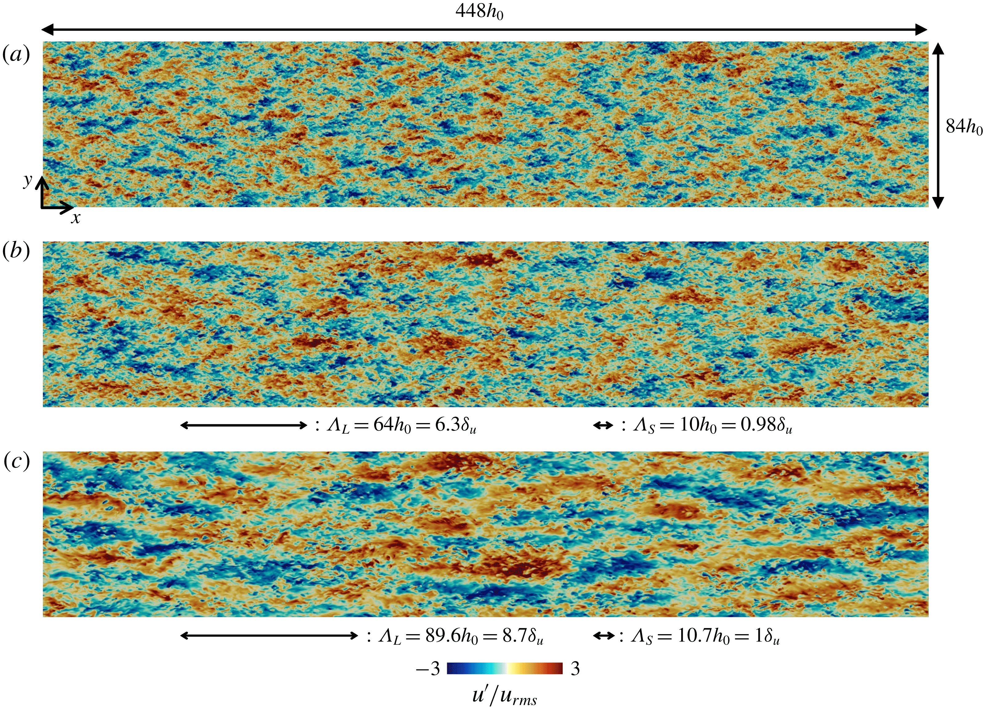
Streamwise velocity fluctuations on the
 $x$
–
 $y$
plane at the centre of the computational domain (
 $z=0$
) at (a)
 $t=160t_{r}$
, (b)
 $t=240t_{r}$
and (c)
 $t=320t_{r}$
for case Re20Ri6. The arrows under (b) and (c) represent wavelengths
 $\unicode[STIX]{x1D6EC}_{S}$
and
 $\unicode[STIX]{x1D6EC}_{L}$
at which the spectra of the streamwise velocity fluctuations
 $k_{x}E_{uu}$
have peaks (see figure 11).
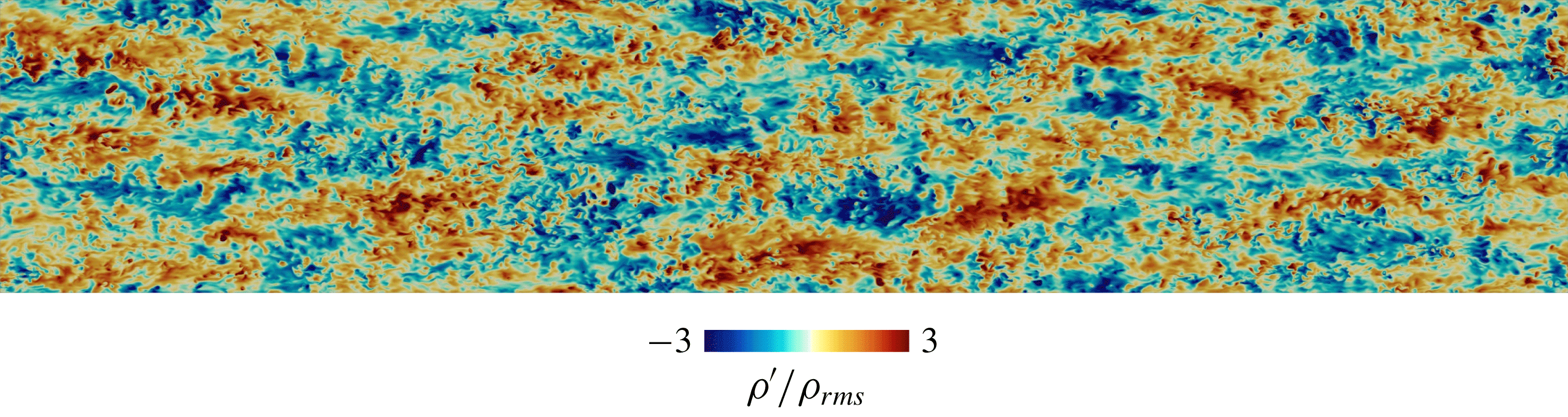
Density fluctuations on the
 $x$
–
 $y$
plane at the centre of the computational domain (
 $z=0$
) at
 $t=320t_{r}$
for case Re20Ri6.
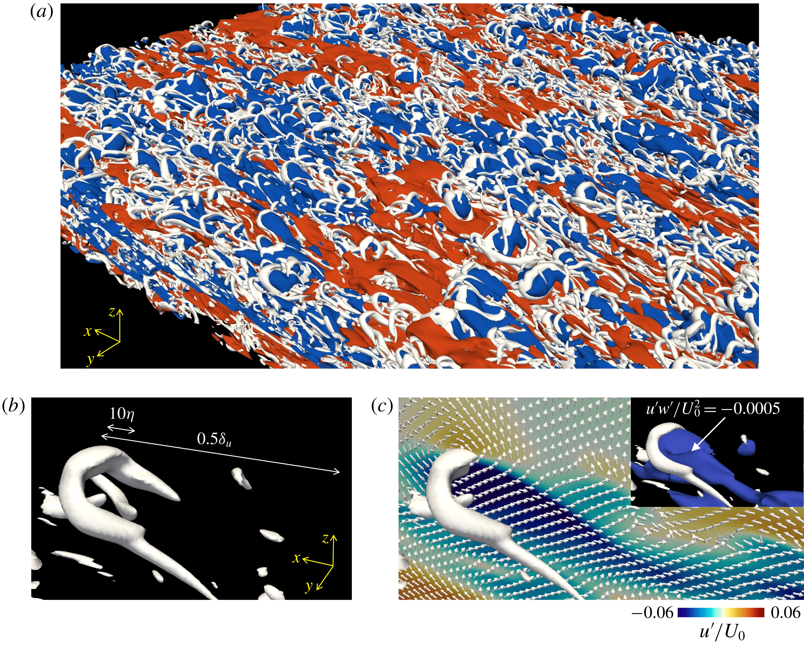
(a) Small-scale vortical structures (white), high-speed (red) regions and low-speed (blue) regions visualized by the isosurface of
 $Q/\langle \unicode[STIX]{x1D61A}_{ij}\unicode[STIX]{x1D61A}_{ij}\rangle _{C}=0.2$
,
 $u^{\prime }/U_{0}=0.039$
and
 $u^{\prime }/U_{0}=-0.039$
, respectively.
 $\langle \unicode[STIX]{x1D61A}_{ij}\unicode[STIX]{x1D61A}_{ij}\rangle _{C}$
is the averaged strain product on the centre line. (b) A hairpin vortex that appears at the top of the stably stratified shear layer. (c) The same hairpin vortex is shown with the colour contours of the streamwise velocity fluctuation
 $u^{\prime }$
and fluctuating velocity vector
 $(u^{\prime },w^{\prime })$
on the
 $x$
–
 $z$
plane crossing the head of the hairpin vortex, where the top right also shows the isosurface of
 $u^{\prime }w^{\prime }=-0.0005U_{0}^{2}$
. These results are taken from Re20Ri6 at
 $t=320t_{r}$
.
(a) Colour contours of the streamwise velocity fluctuation
 $u^{\prime }$
on the
 $x$
–
 $y$
plane at
 $z/h_{0}=0.5$
(
 $z/\unicode[STIX]{x1D6FF}_{u}=0.05$
) and small-scale vortical structures (isosurface of
 $Q/\langle \unicode[STIX]{x1D61A}_{ij}\unicode[STIX]{x1D61A}_{ij}\rangle _{C}=0.2$
) in the region of
 $z/h_{0}\leqslant 2.3$
(
 $z/\unicode[STIX]{x1D6FF}_{u}=0.22$
). (b) Close-up of small-scale vortical structures in the middle of the stably stratified shear layer in (a). These results are taken from Re20Ri6 at
 $t=320t_{r}$
.
Enstrophy in an
 $x$
–
 $z$
plane at (a)
 $t=160t_{r}$
and (b)
 $t=320t_{r}$
for case Re20Ri6.
3.2 Flow structures in stably stratified shear layers
Figure 4(a–c) show the streamwise velocity fluctuations
 $u^{\prime }$
in the horizontal plane at the centre of the shear layer (
 $z=0$
) at different times. The characteristic length scales (e.g.
 $\unicode[STIX]{x1D6EC}_{L}$
defined as the peak wavelength in energy spectra of streamwise velocity fluctuations in figure 11) of
 $u^{\prime }$
grow with time along with the increase in other characteristic length scales of turbulence, such as Kolmogorov scale defined in (2.6). It is also seen that the regions with positive or negative
 $u^{\prime }$
are highly elongated in the streamwise direction at later times. At
 $t=320t_{r}$
, the shear layer thickness is
 $\unicode[STIX]{x1D6FF}_{u}=10.3h_{0}$
, although the regions with positive or negative
 $u^{\prime }$
are extended to streamwise lengths of
 $O(10^{2}h_{0})$
. Figure 5 shows the density fluctuation
 $\unicode[STIX]{x1D70C}^{\prime }$
on the centre plane (
 $z=0$
) at
 $t=320t_{r}$
. The regions with positive or negative
 $\unicode[STIX]{x1D70C}^{\prime }$
are also elongated in the streamwise direction. Comparison between figures 4(c) and 5 shows that
 $u^{\prime }$
tends to be negatively correlated with
 $\unicode[STIX]{x1D70C}^{\prime }$
. This can be explained by the profiles of mean velocity and density.
Small-scale vortical structures are investigated using the second invariant of the velocity gradient tensor,
 $\unicode[STIX]{x1D64C}=(\unicode[STIX]{x1D714}_{i}\unicode[STIX]{x1D714}_{i}-2\unicode[STIX]{x1D61A}_{ij}\unicode[STIX]{x1D61A}_{ij})/4$
, where
 $\unicode[STIX]{x1D714}_{i}$
is the vorticity vector and
 $\unicode[STIX]{x1D61A}_{ij}$
is the rate-of-strain tensor. Regions with
 $Q>0$
are dominated by vortical motions rather than straining motions (Ooi et al.
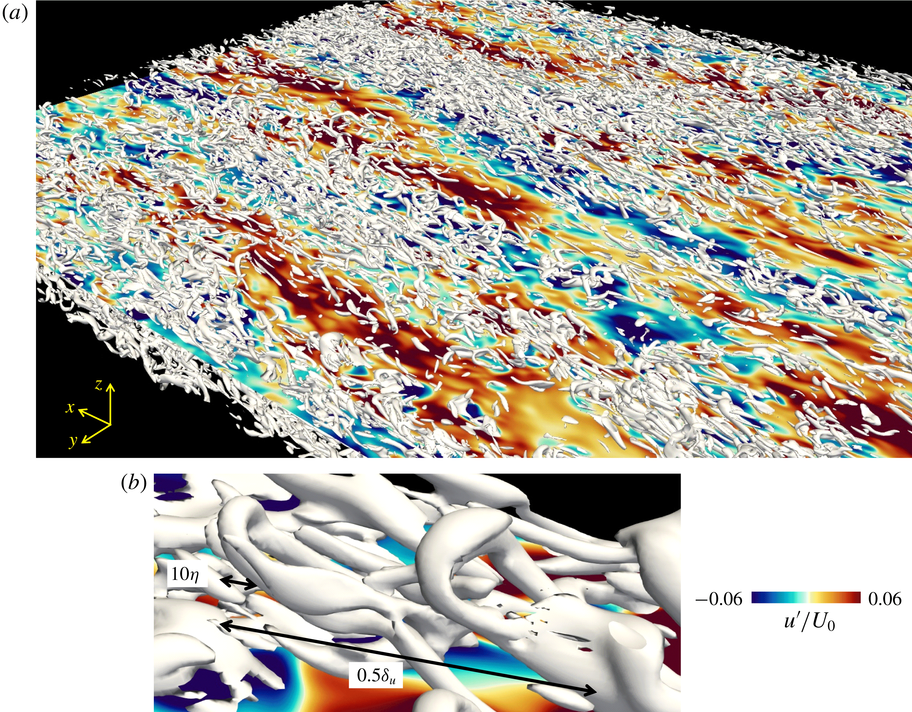
Reference Ooi, Martin, Soria and Chong1999; Davidson Reference Davidson2004). Figure 6(a) shows isosurfaces of a positive value of
 $Q$
(white) along with isosurfaces of positive (red) and negative (blue) values of
 $u^{\prime }$
at the top of the shear layer. Note that the outer edge of the turbulent region appears in the region with
 $0<\unicode[STIX]{x1D6FE}<1$
shown in figure 3(b). One can observe tube-like vortical structures given by the isosurfaces of
 $Q$
in figure 6(a). One of the typical vortical structures in figure 6(a) is enlarged and visualized in figure 6(b). This vortical structure has a shape similar to hairpin vortices found in wall turbulence (Adrian et al.
Reference Adrian, Meinhart and Tomkins2000; Wu & Moin Reference Wu and Moin2009). Most of the vortical structures in figure 6(a) have the shape of a hairpin vortex. A large number of hairpin vortices were also found in turbulent boundary layers at the momentum thickness Reynolds number
 $Re_{\unicode[STIX]{x1D703}}\approx 900$
(Wu & Moin Reference Wu and Moin2009). The diameter of the vortex in figure 6(b) is several times of the Kolmogorov scale
 $\unicode[STIX]{x1D702}$
, which is consistent with small-scale vortical structures of non-stratified turbulence (da Silva, Dos Reis & Pereira Reference da Silva, Dos Reis and Pereira2011). Figure 6(c) shows colour contours of
 $u^{\prime }$
and the velocity fluctuation vector
 $(u^{\prime },w^{\prime })$
on the
 $x$
–
 $z$
plane that crosses the head of the hairpin vortex. The region with low streamwise velocity
 $u^{\prime }<0$
appears between the legs of the hairpin vortex, and is extended in the streamwise direction over a length greater than
 $0.5\unicode[STIX]{x1D6FF}_{u}$
. The vectors also indicate that the head of the hairpin vortex induces a rotating motion, which is also consistent with a velocity vector around the head of the hairpin vortex in wall turbulence (Adrian et al.
Reference Adrian, Meinhart and Tomkins2000). Top right of figure 6(c) shows the isosurface of negative value of
 $u^{\prime }w^{\prime }$
, which can be related to vertical momentum transfer and turbulent kinetic energy production. The region of
 $u^{\prime }w^{\prime }<0$
appears below the head of the hairpin and between the legs, as expected for the hairpin vortex (Davidson Reference Davidson2004), and has a streamwise length scale that is comparable to the streamwise length of the hairpin vortex structure (
 ${\sim}\unicode[STIX]{x1D6FF}_{u}$
). This streamwise length scale of vertical momentum transfer
 $u^{\prime }w^{\prime }<0$
is much larger than the Ozmidov scale
 $L_{O}$
, as can be found from the relation
 $\unicode[STIX]{x1D6FF}_{u}\gg L_{O}$
at
 $t=320t_{r}$
in figure 2(b). At
 $t=320t_{r}$
, the buoyancy Reynolds number
 $Re_{b}$
is 2.7 on the centre line. It is indicated that the hairpin vortex can cause vertical momentum transfer at large scales even for such a small value of
 $Re_{b}$
.
Figure 7(a) shows isosurfaces (white) of a positive value of
 $Q$
in the middle of the shear layer (
 $z\leqslant 0.22\unicode[STIX]{x1D6FF}_{u}$
) along with colour contours of
 $u^{\prime }$
in the horizontal plane at
 $z=0.02\unicode[STIX]{x1D6FF}_{u}$
. Tube-like vortical structures can be found even in the middle of the shear layer for the isosurfaces of
 $Q$
. Figure 7(b) shows a close-up of the vortical structures in the middle of the layer. One can also find hairpin vortices near the centre line. Their diameters are
 ${\sim}10\unicode[STIX]{x1D702}$
and streamwise lengths
 ${\sim}\unicode[STIX]{x1D6FF}_{u}$
, and the vortices are similar in the top and middle of the layer. The middle of the shear layer, shown in figure 7(b), has more vortices oriented in the streamwise direction than in the top of the shear layer, while the top of the shear layer has many heads (spanwise vortices) of the hairpin vortex, as seen in figure 6(a). Comparison between figures 6 and 7 shows that hairpin vortices are more prominent near the top of the shear layer than in the middle.
In figures 6(a) and 7(a), the distribution of the small-scale vortical structures with
 $Q>0$
is intermittent. Specifically, in figure 6(a), small-scale vortical structures appear over the region with negative
 $u^{\prime }$
(blue). Both turbulent and non-turbulent fluids coexist at the top of the shear layer. The fluid with
 $u^{\prime }<0$
below the hairpin vortices in figure 6(a) is turbulent and has lower streamwise velocity than the non-turbulent fluid. On the other hand, the high-speed fluid in figure 6(a) is non-turbulent with negligible enstrophy
 $Q\approx -\unicode[STIX]{x1D61A}_{ij}\unicode[STIX]{x1D61A}_{ij}/2\leqslant 0$
. Therefore, small-scale vortices appear in the turbulent region with negative
 $u^{\prime }$
. Even in the middle of the shear layer in figure 7(a), fewer small-scale vortical structures appear above the region with
 $u^{\prime }>0$
(red). This is similar to the small-scale vortices that appear along with low-speed fluid in turbulent boundary layers (Dennis & Nickels Reference Dennis and Nickels2011).
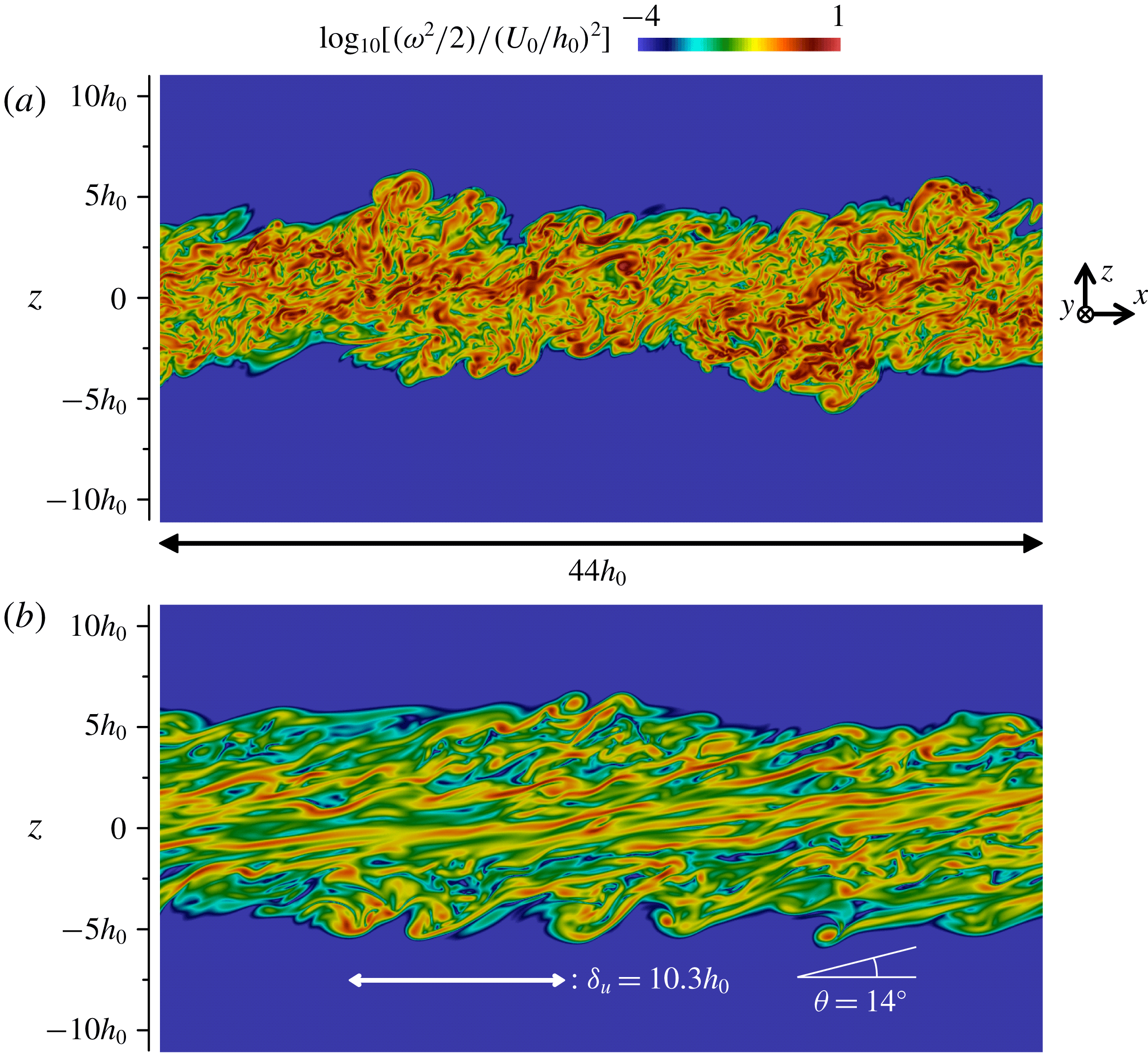
Figure 8 shows the enstrophy
 $\unicode[STIX]{x1D714}_{i}\unicode[STIX]{x1D714}_{i}/2$
in an
 $x$
–
 $z$
plane at
 $t=160t_{r}$
and
 $320t_{r}$
. The region with large enstrophy does not align in a specific direction at
 $t=160t_{r}$
, and the vortical structures with large enstrophy are oriented in various directions. On the other hand, the colour contours of
 $\unicode[STIX]{x1D714}_{i}\unicode[STIX]{x1D714}_{i}/2$
at
 $t=320t_{r}$
show patterns of streamwise vortices in the middle of the shear layer and of the heads and legs of hairpin vortices near the edge of the shear layers. In figure 8(b), the streamwise vortices and the legs of hairpin vortices appear as thin and long regions of large
 $\unicode[STIX]{x1D714}_{i}\unicode[STIX]{x1D714}_{i}/2$
with the streamwise length of
 ${\sim}\unicode[STIX]{x1D6FF}_{u}$
, while the heads of hairpin vortices can be identified as circular regions of large
 $\unicode[STIX]{x1D714}_{i}\unicode[STIX]{x1D714}_{i}/2$
. One of the large enstrophy regions associated with a hairpin vortex makes an angle of 14 degrees with the streamwise direction as shown in figure 8(b). Thus, the hairpin vortex in this stably stratified layer makes a lower angle than analogous vortices in wall turbulence, where the hairpin vortex is often oriented at 45 degrees from the mean flow direction (Head & Bandyopadhyay Reference Head and Bandyopadhyay1981). Reduction of the angle of hairpin vortices due to stable stratification was also reported in experiments of stably stratified boundary layers (Williams Reference Williams2014).
Volume fraction of vortices in turbulent regions,
 $F_{V}$
, plotted as a function of
 $z/\unicode[STIX]{x1D6FF}_{u}$
, where vortices and turbulent regions are detected respectively by the conditions
 $Q/\langle \unicode[STIX]{x1D61A}_{ij}\unicode[STIX]{x1D61A}_{ij}\rangle _{C}\geqslant 0.2$
and
 $|\unicode[STIX]{x1D74E}|\geqslant 0.04\langle |\unicode[STIX]{x1D74E}|\rangle _{C}$
. (a) Time dependence of
 $F_{V}$
in Re20Ri6. (b) In all simulations
 $F_{V}$
at
 $t=320t_{r}$
.
Probability density functions (p.d.f.s) of
 $\text{cos}\unicode[STIX]{x1D703}_{\unicode[STIX]{x1D714}i}=\unicode[STIX]{x1D714}_{i}/|\unicode[STIX]{x1D74E}|$
(
 $i=x,y$
or
 $z$
) computed from the regions with
 $Q/\langle \unicode[STIX]{x1D61A}_{ij}\unicode[STIX]{x1D61A}_{ij}\rangle _{C}\geqslant 0.3$
. The angle between the
 $i$
axis and vorticity vector is represented by
 $\unicode[STIX]{x1D703}_{\unicode[STIX]{x1D714}i}$
. (a)
 $\text{cos}\unicode[STIX]{x1D703}_{\unicode[STIX]{x1D714}x}$
, (c)
 $\text{cos}\unicode[STIX]{x1D703}_{\unicode[STIX]{x1D714}y}$
and (e)
 $\text{cos}\unicode[STIX]{x1D703}_{\unicode[STIX]{x1D714}z}$
at
 $t=160t_{r}$
. (b)
 $\text{cos}\unicode[STIX]{x1D703}_{\unicode[STIX]{x1D714}x}$
, (d)
 $\text{cos}\unicode[STIX]{x1D703}_{\unicode[STIX]{x1D714}y}$
and (f)
 $\text{cos}\unicode[STIX]{x1D703}_{\unicode[STIX]{x1D714}z}$
at
 $t=320t_{r}$
.
In figures 6 and 7, the vortices are detected as the regions with
 $Q/\langle \unicode[STIX]{x1D61A}_{ij}\unicode[STIX]{x1D61A}_{ij}\rangle _{C}\geqslant 0.2$
. The volume occupied by the vortices can be computed with a function
 $I_{Q}$
which is equal to
 $1$
for
 $Q/\langle \unicode[STIX]{x1D61A}_{ij}\unicode[STIX]{x1D61A}_{ij}\rangle _{C}\geqslant 0.2$
and
 $0$
for
 $Q/\langle \unicode[STIX]{x1D61A}_{ij}\unicode[STIX]{x1D61A}_{ij}\rangle _{C}<0.2$
. The volume fraction of the vortices in the turbulent region is computed with the intermittency factor
 $\unicode[STIX]{x1D6FE}=\langle I\rangle$
as
 $F_{V}(z)=\langle I_{Q}\rangle /\unicode[STIX]{x1D6FE}$
, where the vertical profiles of
 $\unicode[STIX]{x1D6FE}$
is shown in figure 3(b). Here,
 $F_{V}$
is computed in the region of
 $\unicode[STIX]{x1D6FE}\geqslant 0.05$
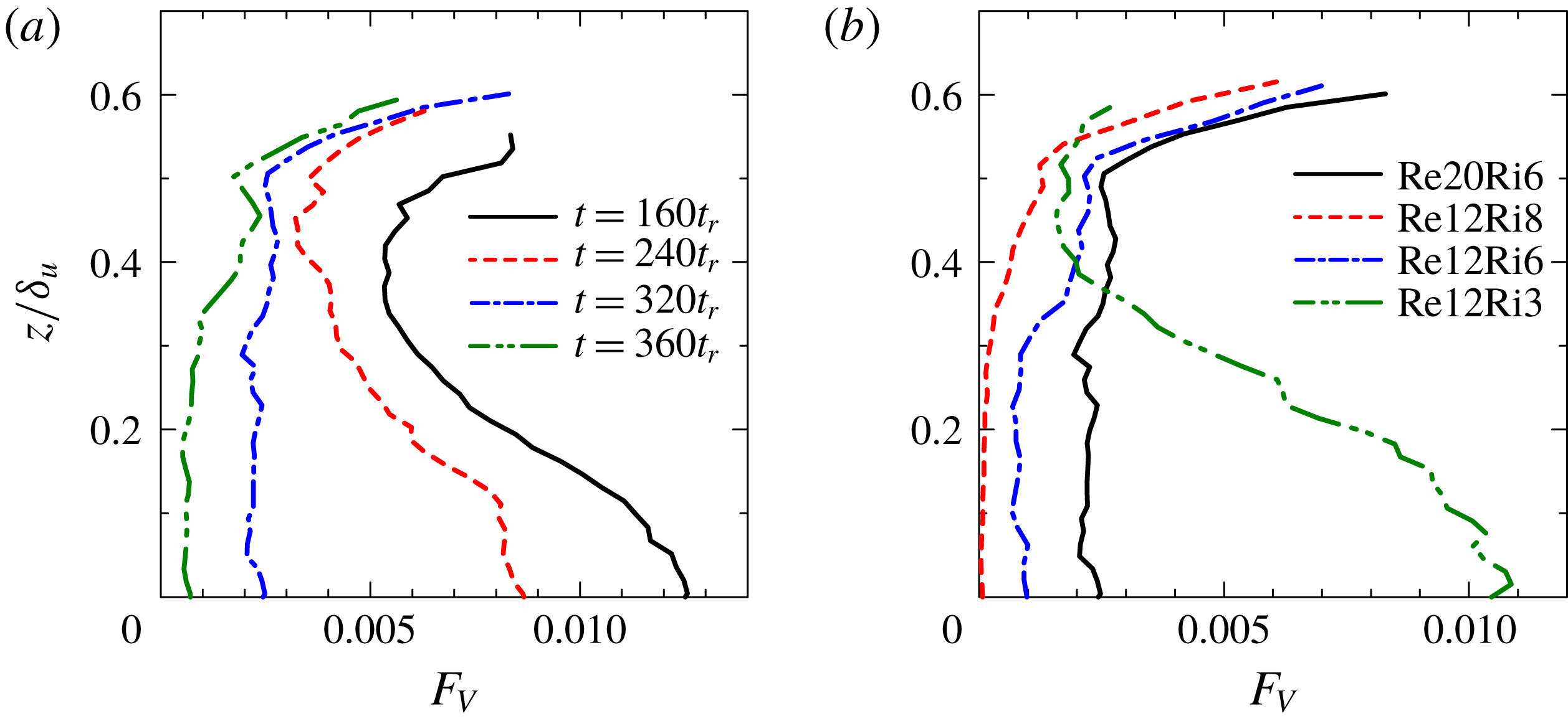
. Figure 9(a) shows the vertical profiles of
 $F_{V}$
at different times in Re20Ri6. Also
 $F_{V}$
is small because the distribution of the vortices is intermittent in space. Less than one per cent of the middle of the shear layer is occupied by the vortices except at early time
 $t=160t_{r}$
.
 $F_{V}$
in the middle of the shear layer is large at
 $t=160t_{r}$
, but decreases with time. At later times (
 $t=320t_{r}$
and
 $360t_{r}$
),
 $F_{V}$
hardly depends on the vertical location in the middle of the shear layer. At these times,
 $F_{V}$
increases with
 $z$
for
 $z/\unicode[STIX]{x1D6FF}_{u}\geqslant 0.5$
. Therefore, the vortices occupy a larger volume of the turbulent region near the edge of the shear layer than the middle of the shear layer. Figure 9(b) shows
 $F_{V}$
at
 $t=320t_{r}$
in all simulations. As
 $Re$
decreases or
 $Ri$
increases,
 $F_{V}$
near the centre line becomes smaller. Comparing figure 9(b) with table 1, one can see that
 $F_{V}$
on the centre line tends to be smaller as
 $Re_{b}$
decreases. Both
 $F_{V}$
and
 $Re_{b}$
decrease with time for the time period shown in figure 9(a). Thus, the volume fraction of the small-scale vortices decreases in the middle of the shear layer as
 $Re_{b}$
decreases. Even after
 $F_{V}$
becomes very small in the middle of the shear layer,
 $F_{V}$
for
 $z/\unicode[STIX]{x1D6FF}_{u}\geqslant 0.5$
has larger values than in the middle. The small-scale vortices in the middle of the shear layer tend to disappear as
 $Re_{b}$
decreases while the vortices can survive for longer time near the edge of the shear layer. Although
 $F_{V}$
depends on the threshold used for defining the vortices, the results are qualitatively insensitive to the threshold, where the dependence of
 $F_{V}$
on time,
 $Re$
and
 $Ri$
observed in figure 9 does not change with the threshold.
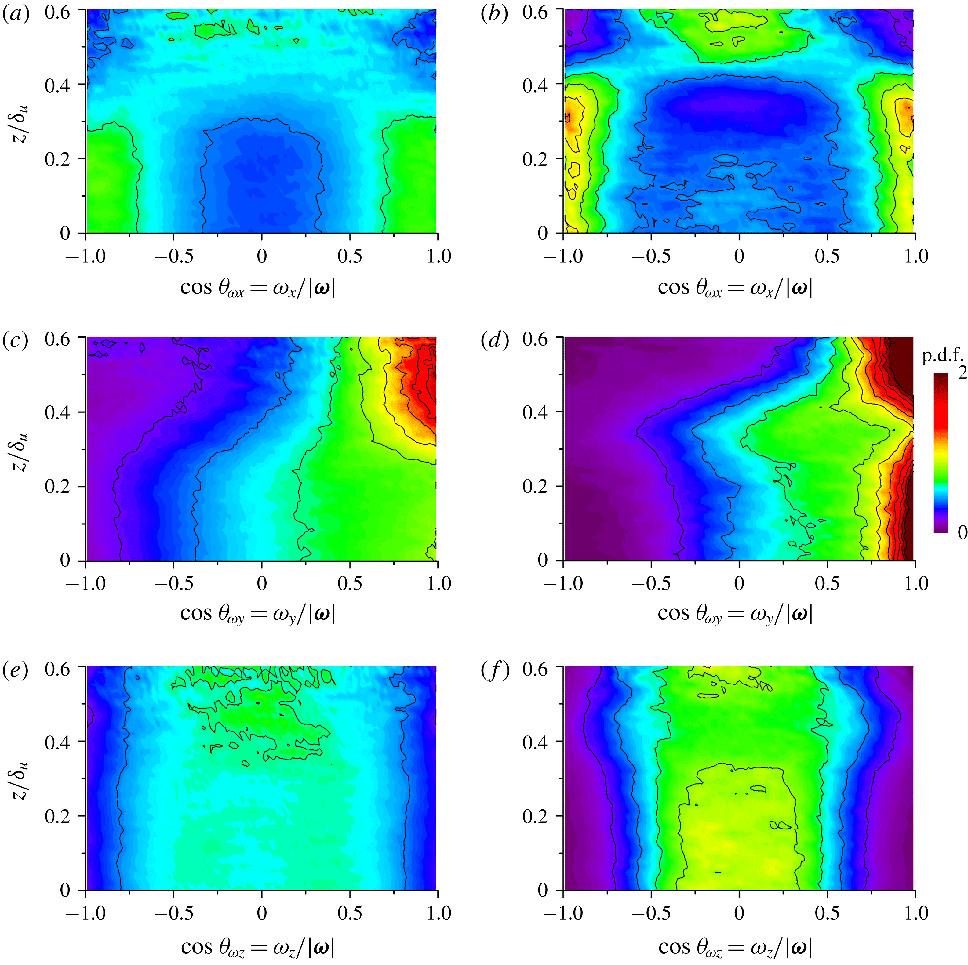
The orientation of vortices is examined by
 $\text{cos}\unicode[STIX]{x1D703}_{\unicode[STIX]{x1D714}i}=\unicode[STIX]{x1D714}_{i}/|\unicode[STIX]{x1D74E}|$
, where
 $\unicode[STIX]{x1D703}_{\unicode[STIX]{x1D714}i}$
is the angle between the
 $i$
axis and the vorticity vector. The probability density functions of
 $\text{cos}\unicode[STIX]{x1D703}_{\unicode[STIX]{x1D714}i}$
are computed from the regions with
 $Q/\langle \unicode[STIX]{x1D61A}_{ij}\unicode[STIX]{x1D61A}_{ij}\rangle _{C}\geqslant 0.3$
, which are inside the isosurfaces used for visualizing the vortices in figures 6 and 7. Figure 10 shows the p.d.f.s of
 $\text{cos}\unicode[STIX]{x1D703}_{\unicode[STIX]{x1D714}x}$
,
 $\text{cos}\unicode[STIX]{x1D703}_{\unicode[STIX]{x1D714}y}$
and
 $\text{cos}\unicode[STIX]{x1D703}_{\unicode[STIX]{x1D714}z}$
at (a,c,e)
 $t=160t_{r}$
and (b,d,f)
 $t=320t_{r}$
. At
 $t=160t_{r}$
and for
 $|z/\unicode[STIX]{x1D6FF}_{u}|\leqslant 0.4$
, the probability density function is large for
 $|\text{cos}\unicode[STIX]{x1D703}_{\unicode[STIX]{x1D714}x}|\geqslant 0.75$
, and the vortices in the middle of the shear layer tend to be oriented in the streamwise direction. The probability density function is large for
 $\text{cos}\unicode[STIX]{x1D703}_{\unicode[STIX]{x1D714}y}>0$
while the probability density function of
 $\text{cos}\unicode[STIX]{x1D703}_{\unicode[STIX]{x1D714}z}$
is somewhat small only for
 $|\text{cos}\unicode[STIX]{x1D703}_{\unicode[STIX]{x1D714}z}|>0.7$
. Thus, vortices can be oriented in various directions although there are a smaller number of vortices aligned in the vertical direction with
 $|\text{cos}\unicode[STIX]{x1D703}_{\unicode[STIX]{x1D714}z}|\approx 1$
. The preference for positive
 $\text{cos}\unicode[STIX]{x1D703}_{\unicode[STIX]{x1D714}y}$
can be related to the mean shear
 $\unicode[STIX]{x2202}\langle u\rangle /\unicode[STIX]{x2202}z>0$
that also contributes to positive spanwise vorticity. A large number of vortices inclined in the streamwise direction were also found in homogenous shear turbulence (Kida & Miura Reference Kida and Miura1998). Therefore, the large probability for
 $|\text{cos}\unicode[STIX]{x1D703}_{\unicode[STIX]{x1D714}x}|\geqslant 0.75$
is caused by the mean shear in the stably stratified shear layer. Near the top of the shear layer at
 $t=160t_{r}$
, the p.d.f.s are large for
 $\text{cos}\unicode[STIX]{x1D703}_{\unicode[STIX]{x1D714}y}\approx 1$
and small for
 $|\text{cos}\unicode[STIX]{x1D703}_{\unicode[STIX]{x1D714}x}|\approx \pm 1$
. Thus, there are a large number of spanwise vortices in this region. The p.d.f.s at
 $t=320t_{r}$
in figure 10(b,d,f) have larger peaks than at
 $t=160t_{r}$
in figure 10(a,c,e): the vortices at a later time tend to align with specific directions, while they can be oriented in various directions at early time, as also confirmed in the visualizations (figure 8). The p.d.f.s for
 $|z/\unicode[STIX]{x1D6FF}_{u}|\leqslant 0.4$
are very large for
 $\text{cos}\unicode[STIX]{x1D703}_{\unicode[STIX]{x1D714}x}\approx \pm 1$
and
 $\text{cos}\unicode[STIX]{x1D703}_{\unicode[STIX]{x1D714}y}\approx 1$
, but are almost 0 for
 $\text{cos}\unicode[STIX]{x1D703}_{\unicode[STIX]{x1D714}z}\geqslant 0.75$
. Most of the vortices are streamwise or spanwise vortices that are almost perpendicular to the vertical direction. Visualizations in figure 7 also show a large number of horizontal vortices. The shape of the p.d.f.s is different near the top of the shear layer, where the p.d.f.s are large for
 $\text{cos}\unicode[STIX]{x1D703}_{\unicode[STIX]{x1D714}y}\approx 1$
and small for
 $\text{cos}\unicode[STIX]{x1D703}_{\unicode[STIX]{x1D714}x}\approx \pm 1$
and
 $\text{cos}\unicode[STIX]{x1D703}_{\unicode[STIX]{x1D714}z}\approx \pm 1$
. Therefore, most small-scale vortices are spanwise vortices at the top of the shear layer. Figure 6 also shows that a large number of the heads of hairpin vortices are oriented in the spanwise direction.
The vortical structures in figure 6 clearly show that there are connections between the stably stratified shear layer and wall-bounded shear flows. This implies that the structures related to the highly elongated pattern of
 $u^{\prime }$
in the
 $x$
–
 $y$
plane in figure 4 are the stably stratified shear layer equivalent to the superstructure or very large-scale motion in wall-bounded shear flows. Flow visualizations related to these structures have been conducted in boundary layers, channel flows and pipe flows (Hutchins & Marusic Reference Hutchins and Marusic2007; Monty et al.
Reference Monty, Stewart, Williams and Chong2007; Hellström et al.
Reference Hellström, Sinha and Smits2011; Lee & Sung Reference Lee and Sung2013), where one can find highly elongated flow structures similar to figure 4(b,c). In turbulent boundary layers, the streamwise extent of the superstructures was found to be of the order of 10 times of the boundary layer thickness (Hutchins & Marusic Reference Hutchins and Marusic2007). The region of positive and negative
 $u^{\prime }$
in figure 4(c) also has a streamwise length of
 $O(10\unicode[STIX]{x1D6FF}_{u})$
. We use the term ‘superstructure’ to denote the structure related to the highly elongated region with positive or negative
 $u^{\prime }$
. It should be noted that the hairpin-shaped vortices cannot be found at earlier times, at which the small-scale vortices can be oriented in various directions as confirmed from figure 8(a). Our previous DNS of stably stratified shear layers (
 $Re=900$
and
 $Ri=0.04$
) also showed that small-scale vortices visualized with
 $Q$
are randomly oriented at early time
 $t=150t_{r}$
, at which the buoyancy Reynolds number is
 $80$
(Watanabe et al.
Reference Watanabe, Riley and Nagata2016). The superstructures also become detectable in figure 4 only for
 $t\geqslant 240t_{r}$
. The structures of stably stratified shear layers at late times become similar to those in wall-bounded shear flows.
In Smyth & Moum (Reference Smyth and Moum2000a ), a few hairpin vortices can be found in the visualization of enstrophy in the DNS of the stably stratified shear layer with a smaller computational domain than in the present DNS. The present study further confirms that the hairpin vortices are prominent near the top of the shear layer, and they can appear even in the middle of the shear layer. Hairpin vortices were also found in other stably stratified turbulent shear flows. It was shown that hairpin vortices appear in turbulent Holmboe waves of stably stratified shear layers (Smyth & Winters Reference Smyth and Winters2003; Smyth Reference Smyth2006). The Holmboe waves are dominant over the Kelvin–Helmholtz instability for high Richardson numbers, and are not addressed in this study. Pham, Sarkar & Winters (Reference Pham, Sarkar and Winters2012) performed DNS of two parallel stably stratified shear layers, where one of the shear layers develops into turbulence through the Kelvin–Helmholtz instability and interacts with another strongly stratified shear layer. Hairpin vortices were also found in their DNS when the turbulent shear layer begins to interact with the strongly stratified shear layer. Field measurements of stratocumulus clouds (Katzwinkel, Siebert & Shaw Reference Katzwinkel, Siebert and Shaw2012; Malinowski et al. Reference Malinowski, Gerber, Plante, Kopec, Kumala, Nurowska, Chuang, Khelif and Haman2013) found a stably stratified region with a wind shear at the stratocumulus top. In two-dimensional profiles of enstrophy taken from DNS of the stratocumulus top (Mellado, Stevens & Schmidt Reference Mellado, Stevens and Schmidt2014; Mellado Reference Mellado2017), the stably stratified sheared region exhibits enstrophy patterns of hairpin vortices similar to those in figure 8(b). These previous studies indicate that hairpin vortices can exist in various stably stratified shear flows.
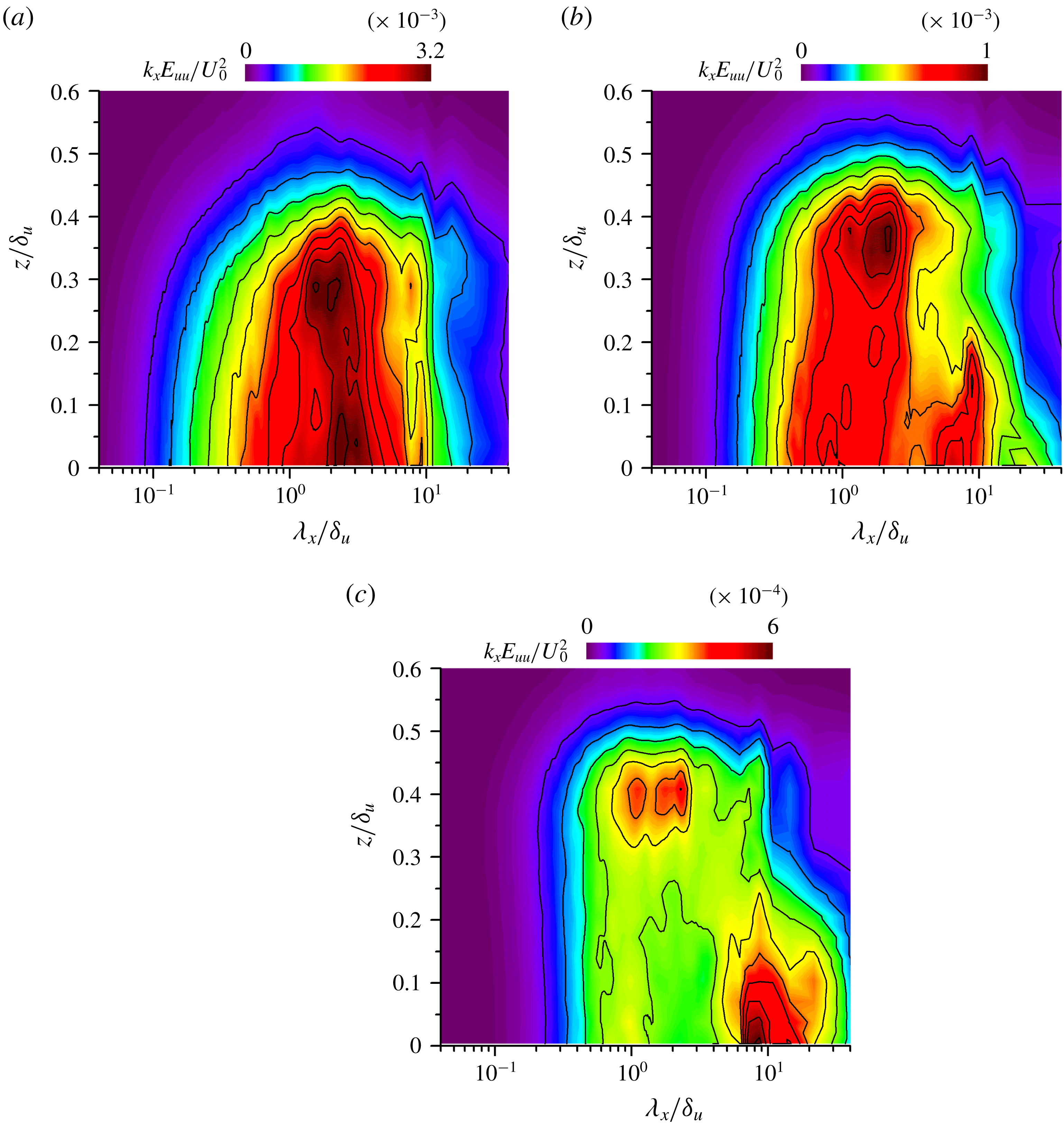
Spectra of streamwise velocity fluctuation
 $k_{x}E_{uu}$
. (a)
 $t=160t_{r}$
, (b)
 $t=240t_{r}$
and (c)
 $t=320t_{r}$
of Re20Ri6. Spectra are shown as a function of the vertical location
 $z$
and the streamwise wavelength
 $\unicode[STIX]{x1D706}_{x}=2\unicode[STIX]{x03C0}/k_{x}$
.
3.3 Spectral analysis
The energy spectrum of the streamwise velocity,
 $E_{uu}$
, is computed using Fourier transforms in the streamwise direction. Figure 11(a–c) show the energy spectrum as functions of the streamwise wavelength
 $\unicode[STIX]{x1D706}_{x}=2\unicode[STIX]{x03C0}/k_{x}$
and the vertical location, where
 $k_{x}$
is the streamwise wavenumber. The spectrum is multiplied by
 $k_{x}$
to put the plots in area-preserving form. It is seen that
 $k_{x}E_{uu}$
substantially changes with time. In figure 11(a), at
 $t=160t_{r}$
,
 $k_{x}E_{uu}$
takes on a very large value at
 $\unicode[STIX]{x1D706}_{x}/\unicode[STIX]{x1D6FF}_{u}\approx 2.0{-}2.5$
. At the later times shown in figures 11(b) and 11(c),
 $k_{x}E_{uu}$
exhibits two peaks at distinct wavelengths for
 $z/\unicode[STIX]{x1D6FF}_{u}\lesssim 0.2$
. At
 $z=0$
in figure 11(c), the shorter wavelength peak occurs at
 $\unicode[STIX]{x1D6EC}_{S}=1.0\unicode[STIX]{x1D6FF}_{u}$
while the longer wavelength peak is found at
 $\unicode[STIX]{x1D6EC}_{L}=8.7\unicode[STIX]{x1D6FF}_{u}$
. The wavelengths
 $\unicode[STIX]{x1D6EC}_{S}$
and
 $\unicode[STIX]{x1D6EC}_{L}$
at
 $z=0$
are shown with arrows in figures 4(b) and 4(c). From these two figures one can see that the streamwise extent of the superstructures is close to the wavelength
 $\unicode[STIX]{x1D6EC}_{L}$
. The shorter wavelength peak, at
 $\unicode[STIX]{x1D6EC}_{S}\sim \unicode[STIX]{x1D6FF}_{u}$
, is close to the shear layer thickness, which is of the same order as the streamwise length of the region of
 $u^{\prime }<0$
near the hairpin vortex in figure 6. Similarly, the spectrum of streamwise velocity with two peaks was also reported in wall turbulence (Guala, Hommema & Adrian Reference Guala, Hommema and Adrian2006; Lee & Moser Reference Lee and Moser2015). In figure 11(c),
 $\unicode[STIX]{x1D6EC}_{L}$
only weakly depends on the vertical location for
 $z/\unicode[STIX]{x1D6FF}_{u}\lesssim 0.2$
. This differs from the spectrum of streamwise velocity in channel and pipe flows, where the peak wavelength
 $\unicode[STIX]{x1D6EC}_{L}$
associated with very large-scale motion becomes larger with the distance from the wall (Monty et al.
Reference Monty, Hutchins, Ng, Marusic and Chong2009). In the region of
 $0.2\leqslant z/\unicode[STIX]{x1D6FF}_{u}\leqslant 0.4$
, the spectral shape in figure 11(c) changes with vertical location from a bimodal profile to a unimodal profile. The peak at
 $\unicode[STIX]{x1D6EC}_{L}$
does not exist near the top of the shear layer (
 $z/\unicode[STIX]{x1D6FF}_{u}\gtrsim 0.3$
), where
 $k_{x}E_{uu}$
is large for
 $\unicode[STIX]{x1D706}_{x}\sim \unicode[STIX]{x1D6FF}_{u}$
. Similarly, the spectrum in turbulent boundary layers has a peak associated with the superstructure near the wall, but this peak disappears in the outer region (Monty et al.
Reference Monty, Hutchins, Ng, Marusic and Chong2009). Although the shorter peak-wavelength
 $\unicode[STIX]{x1D6EC}_{S}$
weakly depends on the vertical location, the peak value of
 $k_{x}E_{uu}$
around
 $\unicode[STIX]{x1D6EC}_{S}$
is higher near the top of the shear layer than in the middle.
Spectra of streamwise velocity fluctuation
 $k_{x}E_{uu}$
on the centre line of Re20Ri6.
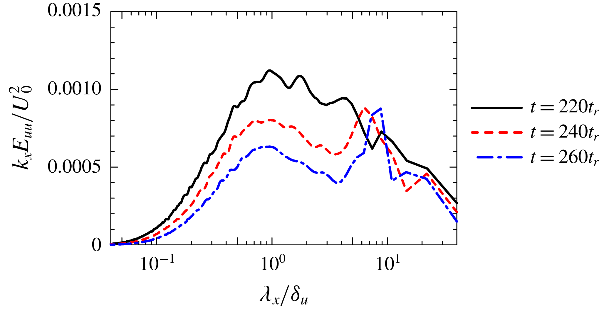
Figure 12 shows
 $k_{x}E_{uu}$
on the centre line at
 $t=220t_{r}$
,
 $240t_{r}$
and
 $260t_{r}$
. The change in the spectral shape occurs between
 $t=220t_{r}$
and
 $240t_{r}$
, and the double peaks discussed above can be seen from
 $t=240t_{r}$
. The shorter peak-wavelength
 $\unicode[STIX]{x1D6EC}_{S}$
divided by
 $\unicode[STIX]{x1D6FF}_{u}$
at
 $t=240t_{r}$
is close to that at later times while the longer peak-wavelength
 $\unicode[STIX]{x1D6EC}_{L}/\unicode[STIX]{x1D6FF}_{u}$
slightly increases with time.
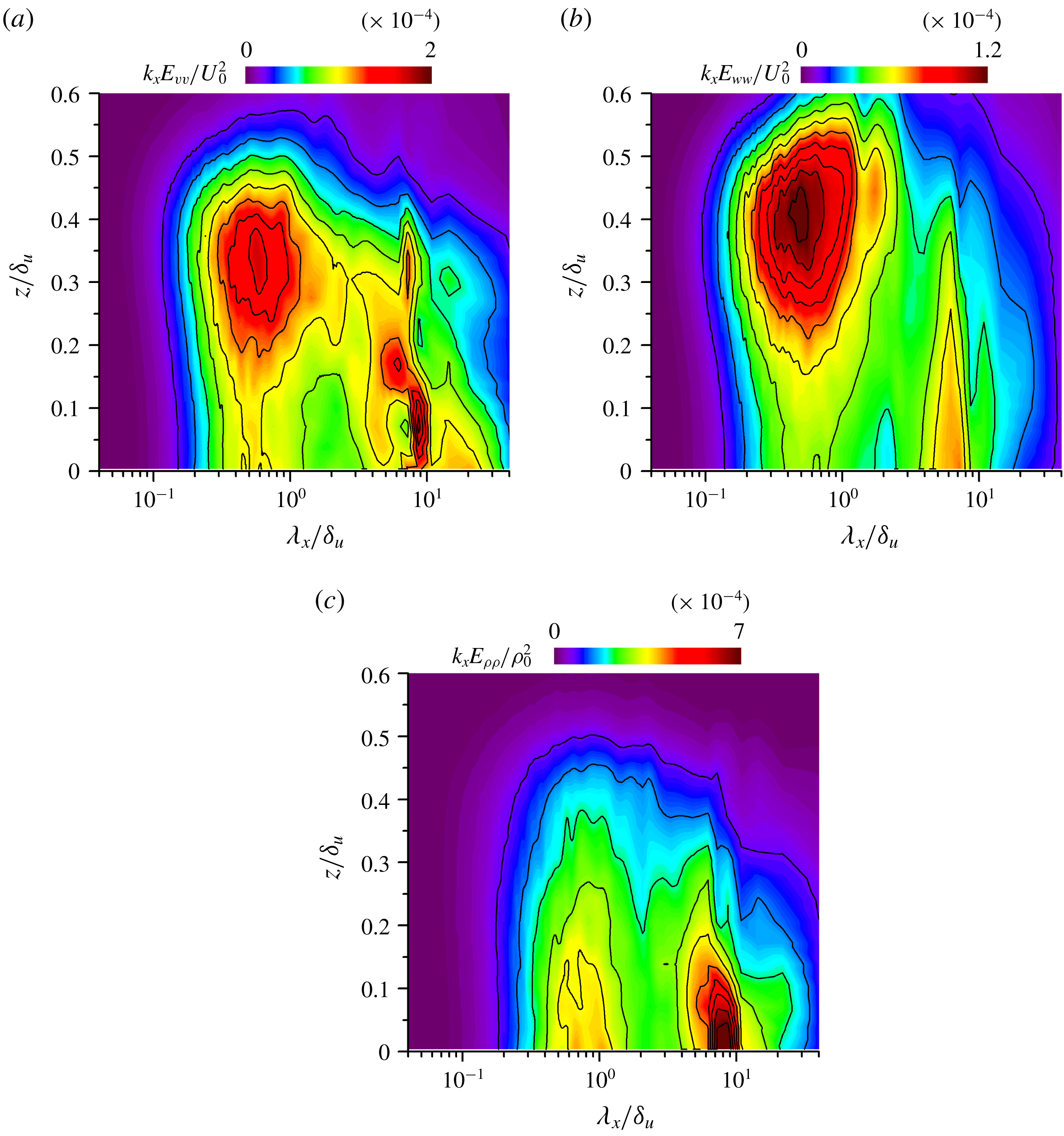
Spectra of (a) spanwise velocity fluctuation
 $k_{x}E_{vv}$
, (b) vertical velocity fluctuation
 $k_{x}E_{ww}$
and (c) density fluctuation
 $k_{x}E_{\unicode[STIX]{x1D70C}\unicode[STIX]{x1D70C}}$
at
 $t=320t_{r}$
of Re20Ri6.
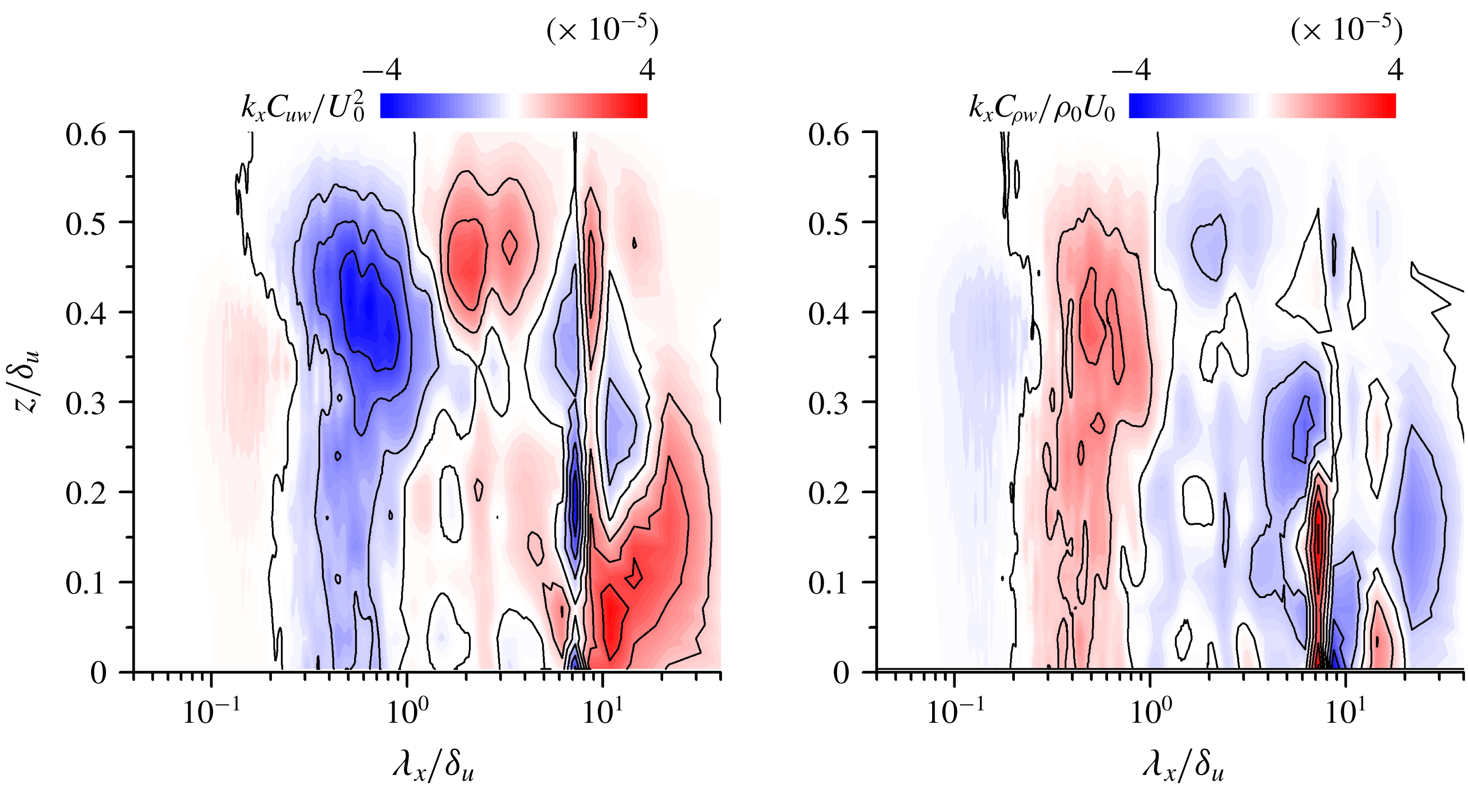
Cospectra of (a) streamwise and vertical velocity fluctuations
 $k_{x}C_{uw}$
, and (b) of the density and vertical velocity fluctuations
 $k_{x}C_{\unicode[STIX]{x1D70C}w}$
at
 $t=320t_{r}$
of Re20Ri6.
Energy spectra of the spanwise velocity, the vertical velocity and the density at
 $t=320t_{r}$
are shown in figures 13(a), 13(b) and 13(c), respectively. Double peaks in these spectra can be seen in the middle of the shear layer. Near the top of the shear layer (
 $z/\unicode[STIX]{x1D6FF}_{u}\approx 0.4$
), a relatively large amount of the energy of the vertical velocity is at the scale of
 $\unicode[STIX]{x1D706}_{x}/\unicode[STIX]{x1D6FF}_{u}\approx 0.5$
, and the vertical motion is still active even at large scales. This is even though this scale is much larger than the Ozmidov scale, which is often interpreted as the largest horizontal scale that can overturn (Riley & Lindborg Reference Riley and Lindborg2008). The peaks in
 $k_{x}E_{vv}$
and
 $k_{x}E_{ww}$
appear at
 $\unicode[STIX]{x1D706}_{x}/\unicode[STIX]{x1D6FF}_{u}\approx 0.5$
on the centre line. This length is about half of the shorter peak-wavelength
 $\unicode[STIX]{x1D706}_{x}/\unicode[STIX]{x1D6FF}_{u}\approx 1.0$
in
 $k_{x}E_{uu}$
. The peak wavelengths of
 $k_{x}E_{vv}$
and
 $k_{x}E_{ww}$
are related to the transverse integral length scale while that of
 $k_{x}E_{uu}$
is related to the longitudinal integral length scale. In homogeneous isotropic turbulence, the transverse integral length scale
 $L_{T}$
is half of the longitudinal one
 $L$
(Pope Reference Pope2000).
 $L_{T}/L$
is about 0.4 even in a turbulent circular jet (Antonia & Zhao Reference Antonia and Zhao2001). This ratio can explain the observed difference in the peak wavelength in
 $k_{x}E_{uu}$
,
 $k_{x}E_{vv}$
and
 $k_{x}E_{ww}$
.
Figures 14(a) and 14(b) show the cospectra at
 $t=320t_{r}$
between
 $u^{\prime }$
and
 $w^{\prime }$
(
 $C_{uw}$
) and between
 $\unicode[STIX]{x1D70C}^{\prime }$
and
 $w^{\prime }$
(
 $C_{\unicode[STIX]{x1D70C}w}$
), whose corresponding integrals give the vertical turbulent fluxes of streamwise momentum
 $\langle u^{\prime }w^{\prime }\rangle$
and density
 $\langle \unicode[STIX]{x1D70C}^{\prime }w^{\prime }\rangle$
. It should be noted that negative
 $u^{\prime }w^{\prime }$
and positive
 $\unicode[STIX]{x1D70C}^{\prime }w^{\prime }$
are associated with a flux of heavier fluid with negative streamwise velocity from the lower side of the shear layer to the upper side, and vice versa. In non-stratified turbulent shear layers, turbulent motions generally contribute to negative
 $u^{\prime }w^{\prime }$
and positive
 $\unicode[STIX]{x1D70C}^{\prime }w^{\prime }$
(Rogers & Moser Reference Rogers and Moser1994). For
 $\unicode[STIX]{x1D706}_{x}/\unicode[STIX]{x1D6FF}_{u}\approx 0.5$
, all vertical locations have
 $C_{uw}<0$
and
 $C_{\unicode[STIX]{x1D70C}w}>0$
, and turbulent mixing is very active at this length scale. This wavelength is also close to the streamwise length of the hairpin vortices, which is associated with the region of
 $u^{\prime }w^{\prime }<0$
in figure 6(c). The velocity vectors in figure 6(c) indicate that the heads of the hairpin vortices can contribute to
 $u^{\prime }w^{\prime }<0$
. Both signs of
 $C_{uw}$
and
 $C_{\unicode[STIX]{x1D70C}w}$
appear at the wavelength around
 $\unicode[STIX]{x1D6EC}_{L}\approx 9\unicode[STIX]{x1D6FF}_{u}$
. Note that a stably stratified fluid can support the propagation of the internal gravity wave-like motions, for which
 $\unicode[STIX]{x1D70C}^{\prime }w^{\prime }$
can take on both positive or negative values depending on the phase of the wave. Oscillation in buoyancy flux
 $\langle \unicode[STIX]{x1D70C}^{\prime }w^{\prime }\rangle$
has been also observed as the wave-like features in stably stratified turbulence (Venayagamoorthy & Stretch Reference Venayagamoorthy and Stretch2006). Although it is difficult to observe the wave motions directly in the visualizations, very large scales affected by the superstructures might behave like a wave that has both negative and positive values of
 $\unicode[STIX]{x1D70C}^{\prime }w^{\prime }$
and
 $u^{\prime }w^{\prime }$
. The convergence of the cospectra at large scales is not as good as at small scales. The change in sign of the cospectra at large scales can be caused by an insufficient convergence of averages computed with large positive and negative fluctuations of
 $\unicode[STIX]{x1D70C}^{\prime }w^{\prime }$
and
 $u^{\prime }w^{\prime }$
in wavenumber space.
Comparison of energy spectra of streamwise velocity fluctuations
 $k_{x}E_{uu}$
among all DNS at
 $t=320t_{r}$
at (a)
 $z=0$
and (b)
 $z=0.4\unicode[STIX]{x1D6FF}_{u}$
.
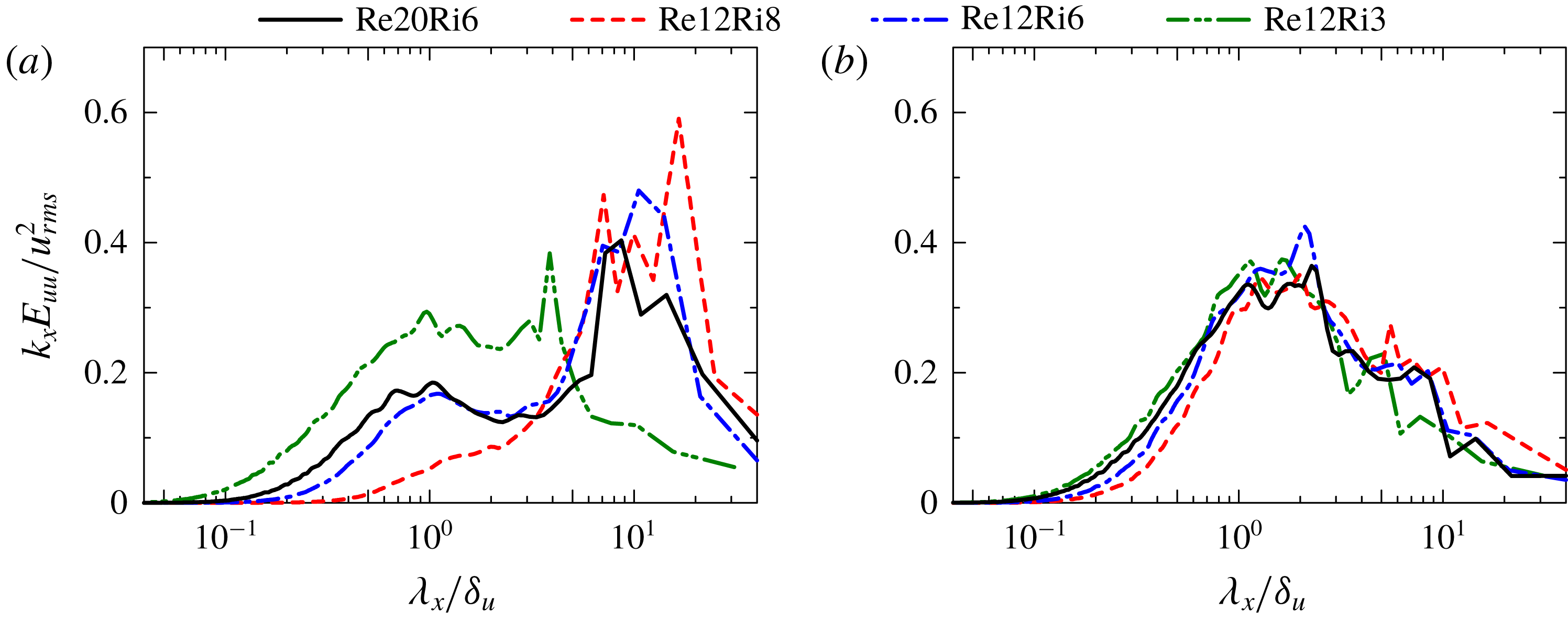
Figures 15(a) and 15(b) compare, for all the simulations, the shape of the spectra
 $k_{x}E_{uu}$
normalized by
 $u_{rms}^{2}$
at
 $z=0$
and
 $z=0.4\unicode[STIX]{x1D6FF}_{u}$
for
 $t=320t_{r}$
. Values of
 $\unicode[STIX]{x1D6FF}_{u}$
,
 $L_{O}$
,
 $\unicode[STIX]{x1D702}$
,
 $Re_{b}$
and
 $Ri_{g}$
at
 $z=0$
and
 $t=320t_{r}$
are summarized in table 1. In figure 15(a), the large peak for
 $\unicode[STIX]{x1D706}_{x}/\unicode[STIX]{x1D6FF}_{u}>1$
appears in all the simulations, but the peak wavelength differs for Re12Ri3, which has the lowest Richardson number. In contrast, the spectra at
 $z=0.4\unicode[STIX]{x1D6FF}_{u}$
have a qualitatively similar shape for all simulations as seen in figure 15(b), where the peak wavelength
 $\unicode[STIX]{x1D6EC}_{S}$
can be related to the streamwise length of the hairpin vortex structures. At both vertical locations, one can also see that the fraction of the energy in small scales,
 $\unicode[STIX]{x1D706}_{x}<\unicode[STIX]{x1D6FF}_{u}$
, decreases as
 $Ri$
increases or
 $Re$
decreases. The energy distribution in the spectral space at
 $z=0$
depends strongly on
 $Re$
and
 $Ri$
. In particular, the scales smaller than
 $\unicode[STIX]{x1D6FF}_{u}$
in Re12Ri8 have only a small amount of energy at
 $z=0$
. However, the energy fraction at small scales at
 $z=0.4\unicode[STIX]{x1D6FF}_{u}$
for Re12Ri8 is comparable to those in other cases, and the small-scale motions can survive longer near the edge than the middle of the shear layer. Two peaks of
 $k_{x}E_{uu}$
on the centre line are expected to be clearly observed when
 $\unicode[STIX]{x1D6EC}_{S}$
and
 $\unicode[STIX]{x1D6EC}_{L}$
are well separated. The shorter peak-wavelength
 $\unicode[STIX]{x1D6EC}_{S}$
is close to the shear layer thickness
 $\unicode[STIX]{x1D6FF}_{u}$
while the longer peak-wavelength
 $\unicode[STIX]{x1D6EC}_{L}$
divided by
 $\unicode[STIX]{x1D6FF}_{u}$
increases with time in figure 12. In figure 15(a), the longer peak-wavelength
 $\unicode[STIX]{x1D6EC}_{L}/\unicode[STIX]{x1D6FF}_{u}$
is smaller in Re12Ri3 than in other cases. Therefore,
 $\unicode[STIX]{x1D6EC}_{L}/\unicode[STIX]{x1D6EC}_{S}$
becomes larger with time or as
 $Ri$
increases. Figures 12 and 15(a) indicate that as the turbulence decays with time, the peak at
 $\unicode[STIX]{x1D6EC}_{S}$
near the centre line decreases and eventually disappears. This happens at an earlier time for a lower Reynolds number or a higher Richardson number, as confirmed in figure 15(a). The two spectral peaks on the centre line can be found when the short-wavelength peak survives until the scale separation
 $\unicode[STIX]{x1D6EC}_{L}/\unicode[STIX]{x1D6EC}_{S}$
becomes large.
3.4 Integral shear parameter
One of the important and common features when comparing the stably stratified shear layer and wall-bounded shear flows is the production of turbulence by mean shear under circumstances in which vertical motions are suppressed by the buoyancy or by the wall. The time scale of the mean shear is defined by
 $\unicode[STIX]{x1D70F}_{S}=S^{-1}=(\unicode[STIX]{x2202}\langle u\rangle /\unicode[STIX]{x2202}z)^{-1}$
. The turbulent production is related to the coupling between the mean shear and eddies with the integral length scale
 $L_{\unicode[STIX]{x1D700}}=q^{3}/\unicode[STIX]{x1D700}$
and velocity scale
 $q=\langle u_{i}^{\prime }u_{i}^{\prime }\rangle ^{1/2}$
. This coupling can be studied with the time scale ratio of the eddy turnover time
 $L_{\unicode[STIX]{x1D700}}/q$
to
 $\unicode[STIX]{x1D70F}_{S}$
given by
 $S^{\ast }=Sq^{2}/\unicode[STIX]{x1D700}$
, which is called the integral shear parameter (Jiménez Reference Jiménez2018). When
 $S^{\ast }\ll 1$
, the eddies evolve much faster than the shear time scale, and there is very little direct interaction between the eddies and the mean shear. On the other hand, when
 $S^{\ast }\gg 1$
, the evolution of the eddies are strongly influenced by the shear.
(a) Vertical profiles of integral shear parameter
 $S^{\ast }$
. (b)
 $S^{\ast }$
against
 $Re_{b}$
on the centre line in the decay period of
 $Re_{b}$
.
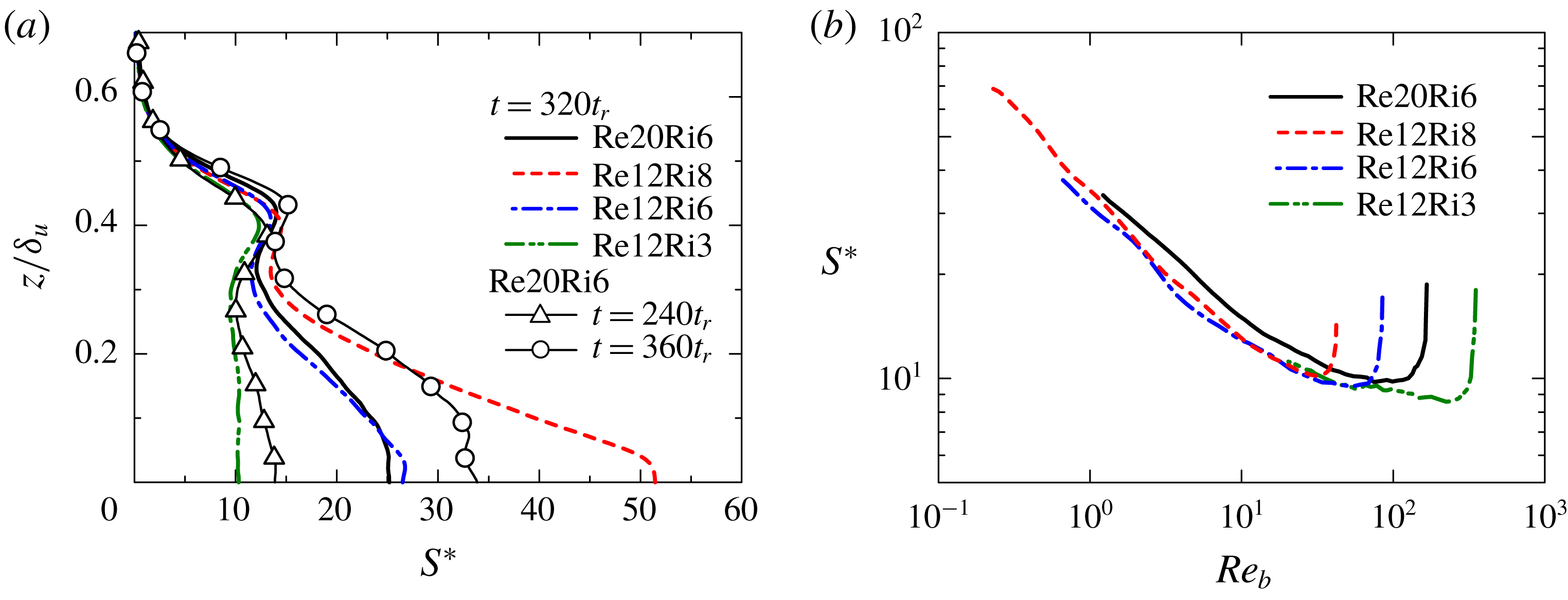
Figure 16(a) shows the vertical profile of
 $S^{\ast }$
in the stably stratified shear layer for the various simulations.
 $S^{\ast }$
in the middle of the shear layer strongly depends on time and
 $Ri$
. One can see from case Re20Ri6 that, in the region near the centre line,
 $S^{\ast }\approx 12{-}14$
until
 $t=240t_{r}$
, and then
 $S^{\ast }$
begins to rapidly increase up to about
 $35$
at
 $t/t_{r}=360$
. Values of
 $S^{\ast }$
near
 $z=0$
also increase as
 $Ri$
increases at
 $t/t_{r}=320$
. Figure 16(b) shows variations of
 $S^{\ast }$
against
 $Re_{b}$
at
 $z=0$
in the decay period of
 $Re_{b}$
. The relation between
 $S^{\ast }$
and
 $Re_{b}$
is similar in all simulations:
 $S^{\ast }\approx 10$
for
 $Re_{b}\gtrsim 10$
, and
 $S^{\ast }$
begins to increase with the decay of
 $Re_{b}$
. In contrast, in the region near the top of the layer (
 $z/\unicode[STIX]{x1D6FF}_{u}\gtrsim 0.35$
)
 $S^{\ast }\approx 13$
independently of time,
 $Re$
and
 $Ri$
. Once
 $S^{\ast }$
increases near the centre line, the vertical variation in
 $S^{\ast }$
becomes similar to those in wall-bounded shear flows, where
 $S^{\ast }$
decreases from the buffer layer with
 $S^{\ast }\approx 30{-}40$
to the logarithmic layer with
 $S^{\ast }\approx 10$
(Jiménez Reference Jiménez2013). The hairpin vortices and superstructures are found in the stably stratified shear layer after
 $S^{\ast }$
on the centre line has begun to increase for
 $t\geqslant 240t_{r}$
. A similar value
 $S^{\ast }\approx 10$
is also obtained in statistically stationary and homogeneous shear turbulence, whose connection to the logarithmic layer is pointed out in Sekimoto, Dong & Jiménez (Reference Sekimoto, Dong and Jiménez2016). Table 1 summarizes
 $L_{\unicode[STIX]{x1D700}}$
at
 $z=0$
at
 $t/t_{r}=320$
. Also,
 $L_{\unicode[STIX]{x1D700}}$
is slightly smaller than
 $\unicode[STIX]{x1D6FF}_{u}$
, and is coincident with the scales at which turbulent kinetic energy and density fluctuations are produced (
 $C_{uw}<0$
and
 $C_{\unicode[STIX]{x1D70C}w}>0$
in figure 14). A moderately large value
 $S^{\ast }\approx 10$
near the top of the shear layer implies that the interaction between the motion at the integral scale and the mean shear is quasilinear in this region (Jiménez Reference Jiménez2018).
4 Conclusions
Direct numerical simulations in a very large computational domain have allowed the investigation of both large-scale and small-scale turbulent structures in stably stratified shear layers. Turbulent structures which appear in stably stratified shear layers at later times are very similar to some of the turbulent structures observed in wall-bounded shear flows. For example, hairpin vortices exist as small-scale vortical structures in the stably stratified shear layers. In the middle of the shear layer, many small-scale vortices are oriented in streamwise or spanwise directions. These streamwise and spanwise vortices can be the legs and heads of the hairpin vortices. On the other hand, a large number of spanwise vortices appear as the heads of the hairpin vortices near the top of the shear layer. The pattern of streamwise velocity fluctuations clearly confirmed the existence of highly elongated structures with positive and negative streamwise velocity fluctuations (superstructures), whose streamwise length scale can be of the order of 10 times the thickness of the stably stratified shear layer. The spectra of velocity and density exhibit large peaks at the wavenumbers associated with the streamwise length of these structures.
It was shown that the superstructures appear in the middle of the shear layer while the hairpin vortices exist in the entire layer. The small-scale vortical structures including hairpin vortices appear intermittently. In the upper side of the shear layer, where the mean streamwise velocity is positive, more small-scale vortical structures appear over the region with negative streamwise velocity fluctuations. The flow patterns associated with hairpin vortices can cause turbulent mixing by transferring heavy fluid from the lower region in the upward direction, and vice versa for lighter fluid. Cospectra related to vertical turbulent fluxes of momentum and density clearly show that turbulent mixing is very active at the length scales close the streamwise extent of the hairpin vortices, although this scale is much larger than the Ozmidov scale.
These structural similarities with wall-bounded shear flows become clearer at later times, when the integral shear parameter
 $S^{\ast }$
begins to increase toward values of about 30 to 50 near the centre line and about 10 near the top of the shear layer. These values of
 $S^{\ast }$
are close to the values of about 30 in the buffer layer and about 10 in the logarithmic layer in wall-bounded shear flows. The value of
 $S^{\ast }$
of about 10 near the edge of the stably stratified shear layer only weakly depends on time and initial Reynolds and Richardson numbers. A large amount of the kinetic energy production occurs at scales close to the shear layer thickness, which is also the length scale of the velocity fluctuations associated with the hairpin vortices.
Acknowledgements
The direct numerical simulations presented in this manuscript were carried out on the high-performance computing system (NEC SX-ACE) in the Japan Agency for Marine-Earth Science and Technology. This work was partially supported by ‘Collaborative Research Project on Computer Science with High-Performance Computing in Nagoya University’ and by JSPS KAKENHI grant number 18K13682 and 18H01367.



