1. Introduction
Compressibility has a strong and complex influence on turbulence and transition in high-speed shear flows. The pre-eminent influence of compressibility is its stabilizing effect on perturbation or fluctuation growth. In turbulent mixing layers, it is well established that compressibility leads to reduced mixing (Chinzei et al. Reference Chinzei, Masuya, Komuro, Murakami and Kudou1986; Papamoschou & Roshko Reference Papamoschou and Roshko1988; Samimy & Elliot Reference Samimy and Elliot1990; Goebel & Dutton Reference Goebel and Dutton1991; Hall, Dimotakis & Rosemann Reference Hall, Dimotakis and Rosemann1993; Clemens & Mungal Reference Clemens and Mungal1995). In these experiments on high-speed mixing layers, the spreading rate decreases with increasing velocity. At low relative Mach numbers, the spreading rates are similar to incompressible values, but the rate decreases significantly with increasing Mach number. The marked reduction of kinetic energy growth rate in homogeneous turbulence has been demonstrated in several studies: direct numerical simulations (DNS) (Sarkar Reference Sarkar1995) and linear analyses (Jackson & Grosch Reference Jackson and Grosch1990; Simone, Coleman & Cambon Reference Simone, Coleman and Cambon1997; Livescu & Madnia Reference Livescu and Madnia2004; Lavin et al. Reference Lavin, Girimaji, Suman and Yu2012).
Several investigations have been performed to understand the stabilizing action of compressibility with increasing Mach number in these shear flows. Sarkar (Reference Sarkar1995) performed DNS of homogeneous shear turbulence at various Mach numbers and showed that pressure plays a pivotal role in stabilizing high-speed shear flows. The study (Sarkar Reference Sarkar1995) clearly identifies pressure–strain correlation as the key phenomenon through which stabilizing physics of compressibility manifests in second-moment closure calculations. This finding was confirmed in Simone et al. (Reference Simone, Coleman and Cambon1997), where the authors further examine the mean shear-induced linear coupling between dilatational and solenoidal velocity fields through rapid distortion theory (RDT). Livescu & Madnia (Reference Livescu and Madnia2004) examined the structure of compressible homogeneous flow using DNS and RDT, focusing on the anisotropy of dilatational and solenoidal fluctuations. Bertsch, Suman & Girimaji (Reference Bertsch, Suman and Girimaji2012) and Lavin et al. (Reference Lavin, Girimaji, Suman and Yu2012) use RDT-generated statistics to categorize and characterize three general types of perturbation evolution depending on the ratio of shear to acoustic time scales characterized by the gradient Mach number. The authors emphasize that the change in character of pressure – from the incompressibility-imposing role in low-speed flows to a genuine thermodynamic variable in high-speed flows – brings about profound changes in pressure–velocity interactions leading to perturbation suppression at high speeds.
At the present time, the central role of pressure–velocity interactions in the stabilization of high-speed shear flow is well recognized. While important progress has been made in characterizing some statistical aspects of the interactions in the above referenced works, deeper understanding is essential for developing closure models and flow control strategies. For incompressible turbulent flows, Mishra & Girimaji (Reference Mishra and Girimaji2010, Reference Mishra and Girimaji2013) demonstrated the importance of characterizing the behaviour of individual perturbation modes not only for achieving comprehensive physical understanding but also for developing accurate predictive turbulence closures and devising effective flow control strategies.
Some mixing-layer investigations in the literature have identified the critical role of obliqueness of the perturbation wavevector with respect to the shear plane (Sandham & Reynolds Reference Sandham and Reynolds1991; Adams & Sandham Reference Adams and Sandham1993; Luo & Sandham Reference Luo, Sandham, Voke, Kleiser and Chollet1994; Kourta & Sauvage Reference Kourta and Sauvage2002; Yao et al. Reference Yao, Krishnan, Sandham and Roberts2007; Wang, Xiaotian & Zhang Reference Wang, Xiaotian and Zhang2013). For example, Sandham & Reynolds (Reference Sandham and Reynolds1991) clearly demonstrated that the perturbation kinetic energy growth depends strongly on the obliqueness angle. They also demonstrated that, while single perturbation modes are generally stable in compressible mixing layers, combinations of oblique and two-dimensional modes show more rapid growth. While the importance of perturbation obliqueness has been recognized, the underlying flow physics is not understood. It is evident that the pressure must play a role, but the manner in which that effect manifests through obliqueness is unknown. Analysing the effect of obliqueness in mixing layers is further exacerbated by the presence of the Kelvin–Helmholtz instability. It may be advantageous to examine first the obliqueness effect in homogeneous shear flows in the absence of any large-scale instability. Thus, in this paper, we will restrict our consideration to homogeneous shear flows. This permits a more detailed analysis of the pressure–velocity interactions to clearly isolate the various effects. Analysis of flows with Kelvin–Helmholtz and Tollmien–Schlichting instabilities will be performed in future studies.
Analysis of individual perturbation mode behaviour in homogeneous compressible shear flows leading to a holistic explanation of the stabilizing mechanism is highly desirable and, as such, is the objective of the present work. This work attempts to bring to fruition the investigations by Livescu & Madnia (Reference Livescu and Madnia2004), Bertsch et al. (Reference Bertsch, Suman and Girimaji2012) and Lavin et al. (Reference Lavin, Girimaji, Suman and Yu2012). Towards this endeavour, we perform DNS and linear analysis of individual and collective behaviour of various perturbation or fluctuation modes in homogeneous shear turbulence. The simulation parameters are the gradient Mach number and initial perturbation mode orientation. The specific objectives of this study are now listed:
-
(a) Characterize the pressure evolution of a given mode as a function of gradient Mach number (
 $M_{g}$
) and perturbation orientation.
-
(b) Examine the velocity perturbation evolution of each mode resulting in characterization of pressure–velocity interactions.
-
(c) Demarcate stable and unstable modes as a function of orientation and Mach number.
-
(d) Develop an explanation of the role of perturbation orientation on stabilization.

To clearly demarcate the role of pressure in the stability phenomenon, the velocity field evolving according to the Burgers equation is also analysed. Comparison of Burgers results with incompressible and compressible Navier–Stokes results will clearly highlight the changing role of pressure with increasing Mach number.
In § 2, we present the governing equations and numerical procedures for RDT and DNS. In § 3, modal analyses of pressure and velocity field are performed. In § 4, we discuss the role of obliqueness and explain the three-stage behaviour. We conclude with a summary of the key results in § 5.
2. Governing equations and numerical approach
The compressible ideal-gas Navier–Stokes equations form the basis of the DNS study:
 $$\begin{eqnarray}\displaystyle & \displaystyle \frac{\partial {\it\rho}}{\partial t}+\frac{\partial ({\it\rho}u_{i})}{\partial x_{i}}=0, & \displaystyle\end{eqnarray}$$
 $$\begin{eqnarray}\displaystyle & \displaystyle \frac{\partial ({\it\rho}u_{i})}{\partial t}+\frac{\partial ({\it\rho}u_{i}u_{j}+p{\it\delta}_{ij})}{\partial x_{j}}=\frac{\partial {\it\sigma}_{ij}}{\partial x_{j}}, & \displaystyle\end{eqnarray}$$
 $$\begin{eqnarray}\displaystyle & \displaystyle \frac{\partial E}{\partial t}+\frac{\partial [(E+p)u_{i}]}{\partial x_{i}}=\frac{\partial ({\it\sigma}_{ij}u_{j})}{\partial x_{i}}-\frac{\partial }{\partial x_{i}}\left({\it\kappa}_{t}\frac{\partial T}{\partial x_{i}}\right). & \displaystyle\end{eqnarray}$$
 ${\it\sigma}_{ij}$
is given by a constitutive relation,
 $$\begin{eqnarray}{\it\sigma}_{ij}={\it\mu}\left[\frac{\partial u_{i}}{\partial x_{j}}+\frac{\partial u_{j}}{\partial x_{i}}\right]+{\it\lambda}{\it\delta}_{ij}\frac{\partial u_{k}}{\partial x_{k}},\end{eqnarray}$$
and the thermodynamic pressure
 $p$
is given by the ideal gas law,
 $$\begin{eqnarray}p={\it\rho}RT.\end{eqnarray}$$
Here,
 ${\it\mu}$
is the coefficient of dynamic viscosity,
 ${\it\kappa}_{t}$
is the thermal conductivity,
 ${\it\lambda}=-{\textstyle \frac{2}{3}}{\it\mu}$
is the second viscosity coefficient and
 $R$
is the gas constant.
For the linear analysis, we decompose the instantaneous fields into background and perturbation fields:
 $$\begin{eqnarray}q=\bar{q}+q^{\prime }.\end{eqnarray}$$
In the context of RDT, this decomposition can be interpreted as mean and fluctuating fields. As pointed out by Sarkar (Reference Sarkar1995), Favre and Reynolds averaged statistics are nearly identical in this limit. Hence, no distinction is made between the two types of statistics.
We restrict ourselves, through the remainder of the paper, to homogeneous shear flows. The mean field variables evolve according to
 $$\begin{eqnarray}\displaystyle & \displaystyle \frac{\partial \overline{{\it\rho}}}{\partial t}+\overline{U_{j}}\frac{\partial \overline{{\it\rho}}}{\partial x_{j}}=-\overline{{\it\rho}}\frac{\partial \overline{U_{j}}}{\partial x_{j}}-\frac{\partial \overline{{\it\rho}^{\prime }{u_{j}}^{\prime }}}{\partial x_{j}}, & \displaystyle\end{eqnarray}$$
 $$\begin{eqnarray}\displaystyle & \displaystyle \frac{\partial \overline{U_{i}}}{\partial t}+\overline{U_{j}}\frac{\partial \overline{U_{i}}}{\partial x_{j}}+\overline{{u_{j}}^{\prime }\frac{\partial {u_{i}}^{\prime }}{\partial x_{j}}}=-\frac{1}{\overline{{\it\rho}}}\frac{\partial \overline{p}}{\partial x_{i}}+\frac{1}{(\overline{{\it\rho}})^{2}}\overline{{\it\rho}^{\prime }\frac{\partial p^{\prime }}{\partial x_{i}}}-\overline{\frac{({\it\rho}^{\prime })^{2}}{(\overline{{\it\rho}})^{3}}}\frac{\partial \overline{p}}{\partial x_{i}}, & \displaystyle\end{eqnarray}$$
 $$\begin{eqnarray}\displaystyle & \displaystyle \frac{\partial \overline{T}}{\partial t}+\overline{U_{j}}\frac{\partial \overline{T}}{\partial x_{j}}+\overline{{u_{j}}^{\prime }\frac{\partial T^{\prime }}{\partial x_{j}}}=-({\it\gamma}-1)\overline{T}\frac{\partial \overline{U_{j}}}{\partial x_{j}}-({\it\gamma}-1)\overline{T^{\prime }\frac{\partial {u_{j}}^{\prime }}{\partial x_{j}}}, & \displaystyle\end{eqnarray}$$
 $$\begin{eqnarray}\displaystyle & \overline{p}=R\overline{{\it\rho}}\overline{T}+R\overline{{\it\rho}^{\prime }T^{\prime }}. & \displaystyle\end{eqnarray}$$
 $$\begin{eqnarray}\overline{U}_{i,j}=S{\it\delta}_{i1}{\it\delta}_{2j},\end{eqnarray}$$
where
 $S$
is the mean shear rate and
 ${\it\delta}_{ij}$
is the Kronecker delta. Here, indices 1 and 2 correspond to the
 $x$
and
 $y$
coordinate axes. This implies that
 $$\begin{eqnarray}\frac{\partial \bar{p}}{\partial x_{i}}=0\quad \text{and}\quad \frac{\partial {\bar{U}}_{i}}{\partial x_{i}}=0.\end{eqnarray}$$
In the linear limit we have
 $$\begin{eqnarray}\overline{{\it\rho}}\approx \overline{{\it\rho}}(0),\quad \overline{T}(t)\approx \overline{T}(0)\quad \text{and}\quad \overline{p}(t)\approx \overline{p}(0).\end{eqnarray}$$
To obtain the fluctuating field equations, we subtract the mean equations, (2.7)–(2.9), from the instantaneous equations, (2.1)–(2.3). At the linear or RDT limit, the fluctuating field equations simplify to (Yu, Girimaji & Luo Reference Yu, Girimaji and Luo2005; Bertsch et al. Reference Bertsch, Suman and Girimaji2012)
 $$\begin{eqnarray}\displaystyle & \displaystyle \frac{\text{d}{\it\rho}^{\prime }}{\text{d}t}=-\overline{{\it\rho}}\frac{\partial {u_{k}}^{\prime }}{\partial x_{k}}, & \displaystyle\end{eqnarray}$$
 $$\begin{eqnarray}\displaystyle & \displaystyle \frac{\text{d}{u_{i}}^{\prime }}{\text{d}t}=-{u_{k}}^{\prime }\frac{\partial \overline{U_{i}}}{\partial x_{k}}-R\frac{\partial T^{\prime }}{\partial x_{i}}-\frac{R\overline{T}}{\overline{{\it\rho}}}\frac{\partial {\it\rho}^{\prime }}{\partial x_{i}}, & \displaystyle\end{eqnarray}$$
 $$\begin{eqnarray}\displaystyle & \displaystyle \frac{\text{d}T^{\prime }}{\text{d}t}=-({\it\gamma}-1)\overline{T}\frac{\partial {u_{k}}^{\prime }}{\partial x_{k}}. & \displaystyle\end{eqnarray}$$
 $$\begin{eqnarray}\displaystyle & \displaystyle \frac{\text{d}\widehat{{\it\rho}}}{\text{d}t}=-\text{i}\bar{{\it\rho}}\widehat{u_{j}}{\it\kappa}_{j}, & \displaystyle\end{eqnarray}$$
 $$\begin{eqnarray}\displaystyle & \displaystyle \frac{\text{d}\widehat{u_{i}}}{\text{d}t}=-\frac{\text{i}}{\bar{{\it\rho}}}\widehat{p}{\it\kappa}_{i}-\widehat{u_{j}}\frac{\partial \overline{U}_{i}}{\partial x_{j}}, & \displaystyle\end{eqnarray}$$
 $$\begin{eqnarray}\displaystyle & \displaystyle \frac{\text{d}\widehat{p}}{\text{d}t}=-\text{i}{\it\gamma}\bar{p}\widehat{u_{j}}{\it\kappa}_{j}, & \displaystyle\end{eqnarray}$$
 $\text{i}=\sqrt{-1}$
is the unit imaginary number,
 $\bar{(\cdot )}$
represents mean flow variables and
 $\hat{(\cdot )}$
represents the fluctuation Fourier amplitude. The evolution equation for the wavevector
 ${\it\kappa}_{i}$
is
 $$\begin{eqnarray}\frac{\text{d}{\it\kappa}_{i}}{\text{d}t}=-{\it\kappa}_{j}\frac{\partial {\bar{U}}_{j}}{\partial x_{i}}.\end{eqnarray}$$
2.1. Pressure-released equations
Burgers equation (or the pressure-released equation) provides further insight into the role of pressure (Simone et al. Reference Simone, Coleman and Cambon1997) when contrasted against the Navier–Stokes flow behaviour. In this linear limit, the Burgers velocity fluctuations evolve according to
 $$\begin{eqnarray}\frac{\text{d}{\hat{u}}_{i}}{\text{d}t}=-{\hat{u}}_{j}\frac{\partial \overline{U_{i}}}{\partial x_{j}}.\end{eqnarray}$$
The kinetic energy in pressure-released homogeneous shear turbulence for an arbitrary mode is given by (Simone et al. Reference Simone, Coleman and Cambon1997)
 $$\begin{eqnarray}\frac{K(t)}{K_{0}}=1+(St)^{2},\quad K=\frac{1}{2}\overline{u_{i}^{\prime }u_{i}^{\prime }},\end{eqnarray}$$
where
 $K_{0}$
is the initial energy. The RDT and linearized Burgers equations will be compared to establish the precise role of pressure in compressible flows. All RDT equations are solved using a standard fourth-order Runge–Kutta scheme. This scheme has been verified in Lavin et al. (Reference Lavin, Girimaji, Suman and Yu2012).
2.2. Direct numerical simulation scheme
The DNS performed in this study employ the gas-kinetic method (GKM). The GKM is a finite-volume-based numerical scheme developed to solve the Boltzmann equation employing the Bhatnagar–Gross–Krook collision operator. The kinetic Boltzmann equation describes the evolution of a single-particle velocity distribution function. The gas-kinetic equation is a first-order integro-partial differential equation with a linear advection term. The fundamental quantity in the gas-kinetic equation is the particle distribution function, from which any of the flow variables of interest, such as density, momentum and energy, can be easily calculated. Details of the numerical solution of gas-kinetic equations can be found in Xu (Reference Xu1998, Reference Xu2001), Xu, Mao & Tang (Reference Xu, Mao and Tang2005), Liao, Peng & Luo (Reference Liao, Peng and Luo2009) and Kumar, Girimaji & Kerimo (Reference Kumar, Girimaji and Kerimo2013). In all simulations, the speed of sound
 $a_{0}$
is taken to be nearly
 $350\ \text{m}\ \text{s}^{-1}$
.
The computational domain is a cubic box of dimension
 $l=2{\rm\pi}$
. The box is discretized into
 $N_{x}\times N_{y}\times N_{z}$
cells with
 $N_{x}=256,N_{y}=256$
and
 $N_{z}=512$
along the
 $x,y$
and
 $z$
directions, respectively. As mentioned earlier, we apply uniform shear such that the gradient of the mean flow field is
 ${\bar{U}}_{i,j}=S{\it\delta}_{i1}{\it\delta}_{2j}$
, where
 $S$
is the shearing rate. For further details on the grid resolution study, the reader is referred to Kumar et al. (Reference Kumar, Girimaji and Kerimo2013).
We perform two types of DNS calculations – initial individual mode and collective perturbations. In modal calculations, the perturbation velocity amplitude and wavenumber vectors are specified as needed. The collective simulations commence from a three-dimensional, random, isotropic and solenoidal
 $(\boldsymbol{{\rm\nabla}}\boldsymbol{\cdot }\boldsymbol{u}=0)$
perturbation velocity field. The initial perturbation fields are similar to those of Sarkar (Reference Sarkar1995). Initially, perturbation energy is restricted to wavenumbers in the range
 ${\it\kappa}\in [{\it\kappa}_{min},{\it\kappa}_{max}]$
. The velocity field is periodic and satisfies a specified one-dimensional energy spectrum (Kerimo & Girimaji Reference Kerimo and Girimaji2007; Yu et al.
Reference Yu, Girimaji and Luo2005),
 $$\begin{eqnarray}E({\it\kappa},0)=\frac{{\hat{u}}_{i}{\hat{u}}_{i}^{\ast }}{4{\rm\pi}{\it\kappa}^{2}}=A{\it\kappa}^{4}\text{e}^{-B{\it\kappa}^{2}},\quad {\it\kappa}(=\sqrt{{\it\kappa}_{1}^{2}+{\it\kappa}_{2}^{2}+{\it\kappa}_{3}^{2}})\in [{\it\kappa}_{min},{\it\kappa}_{max}],\end{eqnarray}$$
where
 $B=0.54$
,
 ${\hat{u}}_{i}$
is the Fourier amplitude and
 ${\hat{u}}_{i}^{\ast }$
is its complex conjugate. The procedure of generating such a field is given in Rogallo (Reference Rogallo1981), Yu et al. (Reference Yu, Girimaji and Luo2005), Lee (Reference Lee2008) and Kumar et al. (Reference Kumar, Girimaji and Kerimo2013). We choose the value of
 $A$
to match the prescribed initial perturbation intensity or equivalently the turbulent Mach number
 $M_{t0}$
. The kinematic viscosity
 ${\it\nu}$
is set to achieve a desired initial Taylor microscale Reynolds number
 $\mathit{Re}_{{\it\lambda}0}$
.
We apply periodic boundary conditions in the
 $x_{1}$
and
 $x_{3}$
directions. For boundaries in
 $x_{2}$
(the shear direction), we apply the shear-periodic boundary condition (Baron Reference Baron1982; Schumann Reference Schumann1985; Gerz, Schumann & Elghobashi Reference Gerz, Schumann and Elghobashi1989; Kreuzinger & Friedrich Reference Kreuzinger, Friedrich, Wagner, Hanke, Bode and Durst2002)
 $$\begin{eqnarray}{\it\phi}(t,x+m_{1}L_{x},y+m_{2}L_{y},z+m_{3}L_{z})={\it\phi}(t,x-Sm_{2}L_{y}t,y,z),\end{eqnarray}$$
where
 $L_{x},L_{y}$
and
 $L_{z}$
are the dimensions of the box along the three coordinate directions, and
 $m_{1},m_{2}$
and
 $m_{3}$
are arbitrary integers. Along the direction of shear, only the fluctuating or perturbation component of velocity is periodic, while the mean velocity is specified to maintain the prescribed shear
 $S$
.
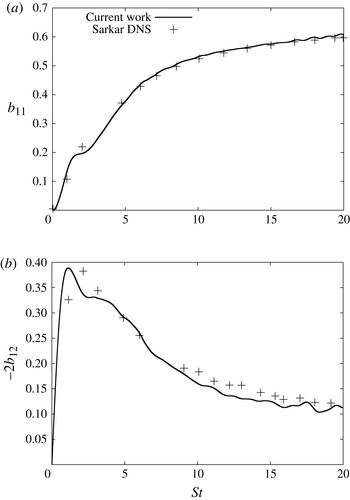
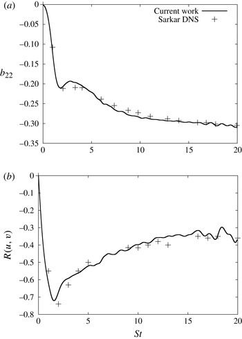
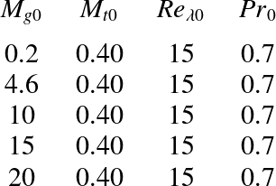
A comprehensive validation of the GKM code in a variety of homogeneous shear and decaying isotropic flows is given in Kumar et al. (Reference Kumar, Girimaji and Kerimo2013). In the aforementioned work, linear and nonlinear flow features are independently verified and validated against asymptotic theories (RDT) and other DNS results. Here, in table 1, we provide one set of comparisons of the present GKM results with the DNS data of Sarkar (Reference Sarkar1995, case A4). In figure 1(a,b) anisotropy components
 $b_{11}$
and
 $b_{12}$
are compared and show excellent agreement between the two DNS schemes. The anisotropy component
 $b_{22}$
in figure 2(a) and the correlation coefficient
 $R(u,v)$
in figure 2(b) also show good agreement.
DNS parameters of the homogeneous shear case A4 of Sarkar (Reference Sarkar1995).

Comparison against DNS case A4 of Sarkar (Reference Sarkar1995): (a)
 $b_{11}=\overline{u_{1}^{\prime }u_{1}^{\prime }}/(2k)-{\textstyle \frac{1}{3}}$
and (b)
 $-2b_{12}$
, where
 $b_{12}=\overline{u_{1}^{\prime }u_{2}^{\prime }}/(2k)$
.

Comparison against DNS case A4 of Sarkar (Reference Sarkar1995): (a)
 $b_{22}=\overline{u_{2}^{\prime }u_{2}^{\prime }}/(2k)-{\textstyle \frac{1}{3}}$
and (b)
 $R(u,v)=\overline{u^{\prime }v^{\prime }}/(u_{rms}^{\prime }v_{rms}^{\prime })$
.

The applicability of the code for simulating individual modes is examined in detail in Kumar et al. (Reference Kumar, Girimaji and Kerimo2013). Dilatational and solenoidal modes are examined individually owing to the fundamental difference in their flow character. Later in this paper, further evidence is provided in figures 9(a) and 10 that the computed solenoidal and dilatational behaviours over a large range of Mach numbers scale according to linear analysis. For computing collections of modes, Kumar et al. (Reference Kumar, Girimaji and Kerimo2013) demonstrate that the simulations are precise for at least
 $\mathit{Re}_{{\it\lambda}}\approx 45$
. The energy budget, spectra, velocity gradient skewness and flatness have been examined in Kumar et al. (Reference Kumar, Girimaji and Kerimo2013). All the modal and collective perturbation behaviours performed in this study are well within the verified limits of the codes’ applicability. Overall, the present GKM has been well validated for this investigation.
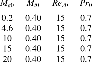
All the collective-mode simulations performed in the current study are listed in table 2. The details of the individual mode DNS are indicated in the respective subsections.
DNS parameters of homogeneous shear cases for a collection of initial mode perturbations.
3. Modal analysis of pressure and velocity fluctuations
With the exception of Livescu & Madnia (Reference Livescu and Madnia2004), most, if not all, previous homogenous shear turbulence investigations focus on the evolution of collective-mode velocity and pressure statistics. The statistics are gleaned from a collection of perturbation modes that are initially distributed in an isotropic manner. While this has led to important advances in our understanding, a comprehensive explanation requires the characterization of individual mode behaviour.
In this section, we present the evolution of pressure and velocity amplitudes of individual modes as a function of initial gradient Mach number and initial wave orientation. This aspect of the present paper builds on the earlier work by Livescu & Madnia (Reference Livescu and Madnia2004). They provide a Bessel function solution to describe the evolution of velocity and pressure amplitude vectors. In this work, we proceed further to clearly demarcate the stability of different perturbation orientations and develop the underlying physical explanation. In compressible shear flows, velocity perturbations evolve under the influence of two competing influences: the applied shear and pressure response. Viscous effects, while present, play a lesser role in the investigated phenomenon.
Let
 $\hat{p}$
be the Fourier amplitude and
 ${\bf\kappa}=({\it\kappa}_{1},{\it\kappa}_{2},{\it\kappa}_{3})$
be the wavevector, with
 ${\it\kappa}=|{\bf\kappa}|$
as the magnitude. It must be pointed out that
 ${\it\kappa}_{1}$
,
 ${\it\kappa}_{2}$
and
 ${\it\kappa}_{3}$
are the wavevector components in the streamwise, stream-normal and spanwise directions. We commence our analysis with the evolution equation for dilatation deduced from (2.18) and (2.20):
 $$\begin{eqnarray}\frac{\text{d}}{\text{d}t}({\hat{u}}_{i}{\it\kappa}_{i})=-\text{i}{\it\kappa}_{i}{\it\kappa}_{i}\frac{\hat{p}}{\bar{{\it\rho}}}-2{\hat{u}}_{j}{\it\kappa}_{i}S_{ij}.\end{eqnarray}$$
For the shear flow under consideration, this can be written as
 $$\begin{eqnarray}\frac{\hat{p}}{\bar{{\it\rho}}}=2\text{i}\left[\frac{{\it\kappa}_{1}}{{\it\kappa}^{2}}{\hat{u}}_{2}S\right]+\frac{\text{i}}{{\it\kappa}^{2}}\frac{\text{d}}{\text{d}t}({\hat{u}}_{i}{\it\kappa}_{i}),\end{eqnarray}$$
where
 ${\it\kappa}_{i}{\it\kappa}_{i}={\it\kappa}^{2}$
. The first term on the right-hand side is the only source term in the Poisson equation for pressure in incompressible flows. The second term represents the compressibility effect. From (2.19) the compressible source term can be expressed as
 $$\begin{eqnarray}\text{i}\frac{\text{d}}{\text{d}t}({\hat{u}}_{i}{\it\kappa}_{i})=-\frac{1}{{\it\gamma}\bar{p}}\frac{\text{d}^{2}\hat{p}}{\text{d}t^{2}},\end{eqnarray}$$
as
 $\bar{p}$
is constant. Substituting (3.2) and (3.3) into (2.18), the velocity amplitude equations can be written as
 $$\begin{eqnarray}\displaystyle & & \displaystyle \displaystyle \frac{\text{d}{\hat{u}}_{1}}{\text{d}t}=u_{2}S\left[\frac{2{\it\kappa}_{1}^{2}}{{\it\kappa}^{2}}-1\right]+\text{i}\frac{{\it\kappa}_{1}}{{\it\kappa}^{2}}\frac{1}{{\it\rho}a_{0}^{2}}\frac{\text{d}^{2}\hat{p}}{\text{d}t^{2}},\end{eqnarray}$$
 $$\begin{eqnarray}\displaystyle & & \displaystyle \displaystyle \frac{\text{d}{\hat{u}}_{2}}{\text{d}t}=u_{2}S\left[\frac{2{\it\kappa}_{1}{\it\kappa}_{2}}{{\it\kappa}^{2}}\right]+\text{i}\frac{{\it\kappa}_{2}}{{\it\kappa}^{2}}\frac{1}{{\it\rho}a_{0}^{2}}\frac{\text{d}^{2}\hat{p}}{\text{d}t^{2}},\end{eqnarray}$$
 $$\begin{eqnarray}\displaystyle & & \displaystyle \displaystyle \frac{\text{d}{\hat{u}}_{3}}{\text{d}t}=u_{2}S\left[\frac{2{\it\kappa}_{1}{\it\kappa}_{3}}{{\it\kappa}^{2}}\right]+\text{i}\frac{{\it\kappa}_{3}}{{\it\kappa}^{2}}\frac{1}{{\it\rho}a_{0}^{2}}\frac{\text{d}^{2}\hat{p}}{\text{d}t^{2}},\end{eqnarray}$$
 ${\it\gamma}\bar{p}={\it\rho}a_{0}^{2}$
. As we approach the incompressible limit, the second term on the right-hand side of (3.4)–(3.6) tends to zero due to an increasingly large acoustic speed (
 $a_{0}\rightarrow \infty$
as
 $M\rightarrow 0$
).
The velocity field evolution equations can also be expressed in terms of the stream-normal velocity and pressure amplitudes:
 $$\begin{eqnarray}\displaystyle & & \displaystyle \displaystyle \frac{\text{d}{\hat{u}}_{2}}{\text{d}t}=-\text{i}\frac{\hat{p}}{\bar{{\it\rho}}}{\it\kappa}_{2},\end{eqnarray}$$
 $$\begin{eqnarray}\displaystyle & & \displaystyle \displaystyle \frac{\text{d}{\hat{u}}_{1}}{\text{d}t}=-u_{2}S-\text{i}\frac{\hat{p}}{\bar{{\it\rho}}}{\it\kappa}_{1}=-u_{2}S+\frac{{\it\kappa}_{1}}{{\it\kappa}_{2}}\frac{\text{d}{\hat{u}}_{2}}{\text{d}t},\end{eqnarray}$$
 $$\begin{eqnarray}\displaystyle & & \displaystyle \displaystyle \frac{\text{d}{\hat{u}}_{3}}{\text{d}t}=-\text{i}\frac{\hat{p}}{\bar{{\it\rho}}}{\it\kappa}_{3}=\frac{{\it\kappa}_{3}}{{\it\kappa}_{2}}\frac{\text{d}{\hat{u}}_{2}}{\text{d}t}.\end{eqnarray}$$
 ${\hat{u}}_{2}$
component. These equations also show how the wavevector orientation has a strong influence on the evolution of the velocity field.
3.1. Pressure field evolution
To fully comprehend the compressibility effect manifesting via pressure, we next investigate the evolution of pressure fluctuations as a function of wavevector direction and Mach number. The linearized non-dimensional transport equation for pressure was derived by Kovasznay (Reference Kovasznay1953) in the context of homogeneous turbulent flows. Livescu & Madnia (Reference Livescu and Madnia2004) extended the linearized equations for homogeneous turbulent shear flows in the RDT limit. Here, for the sake of completeness, we provide a brief derivation. Differentiating (2.19) twice with respect to time:
 $$\begin{eqnarray}\displaystyle & & \displaystyle \displaystyle \frac{\text{d}^{2}\hat{p}}{\text{d}t^{2}}=-\text{i}{\it\gamma}\bar{p}\left[\frac{-\text{i}}{\bar{{\it\rho}}}\hat{p}{\it\kappa}_{j}{\it\kappa}_{j}-2{\hat{u}}_{k}S_{jk}{\it\kappa}_{j}\right],\end{eqnarray}$$
 $$\begin{eqnarray}\displaystyle & & \displaystyle \displaystyle \frac{\text{d}^{3}\hat{p}}{\text{d}t^{3}}=-\frac{{\it\gamma}\bar{p}}{\bar{{\it\rho}}}\left[\frac{\text{d}\hat{p}}{\text{d}t}{\it\kappa}^{2}-4\hat{p}{\it\kappa}_{i}{\it\kappa}_{j}S_{ij}\right].\end{eqnarray}$$
 $$\begin{eqnarray}{\it\kappa}_{i}{\it\kappa}_{j}S_{ij}={\it\kappa}_{1}{\it\kappa}_{2}S,\quad u_{j}{\it\kappa}_{i}S_{ij}=u_{2}{\it\kappa}_{1}S.\end{eqnarray}$$
Using the definition of speed of sound,
 $a_{0}=\sqrt{{\it\gamma}\bar{p}/\bar{{\it\rho}}}$
, and (2.18), we can finally write
 $$\begin{eqnarray}\frac{\text{d}^{3}\hat{p}}{\text{d}t^{3}}=-a_{0}^{2}\left({\it\kappa}^{2}\frac{\text{d}\hat{p}}{\text{d}t}-4{\it\kappa}_{1}{\it\kappa}_{2}S\hat{p}\right).\end{eqnarray}$$
For a more detailed derivation of the evolution equation of pressure in the RDT limit, the reader is referred to Livescu & Madnia (Reference Livescu and Madnia2004).
To develop further insight into the flow physics, we proceed to analyse the effects of orientation and Mach number. Equation (3.13) can be simplified using the evolution equation for the wavenumber vector from (2.20):
 $$\begin{eqnarray}{\it\kappa}_{1}(t)={\it\kappa}_{1}(0)\equiv {\it\kappa}_{1}^{0},\quad {\it\kappa}_{2}(t)={\it\kappa}_{2}(0)-{\it\kappa}_{1}(0)St,\quad {\it\kappa}_{3}(t)={\it\kappa}_{3}(0)\equiv {\it\kappa}_{3}^{0}.\end{eqnarray}$$
We consider three cases based on the orientation of the initial wavevector:
-
(a) Case 1:
${\it\kappa}_{1}=0$
. With
${\it\kappa}_{1}=0$
, the wavevector magnitudes do not grow regardless of
${\it\kappa}_{2}$
and
${\it\kappa}_{3}$
initial values. The pressure field is sinusoidal. -
(b) Case 2:
${\it\kappa}_{2}=0$
. We study this case in detail in the following sections. -
(c) Case 3:
${\it\kappa}_{1},{\it\kappa}_{2},{\it\kappa}_{3}\neq 0$
. In cases with non-zero
${\it\kappa}_{1}$
, after very early transients,
${\it\kappa}_{2}$
quickly grows large enough to make the following approximation:
${\it\kappa}(t)\approx {\it\kappa}_{2}(t)\approx {\it\kappa}_{1}^{0}St$
. Hence, case 3 reduces to case 2 in shear time when
${\it\kappa}_{1}(0)St\gg {\it\kappa}_{2}(0)$
. Therefore the role of
${\it\kappa}_{2}(0)$
is merely to change the virtual time origin.





We now study case 2 (
 ${\it\kappa}_{2}(0)=0$
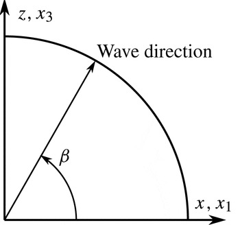
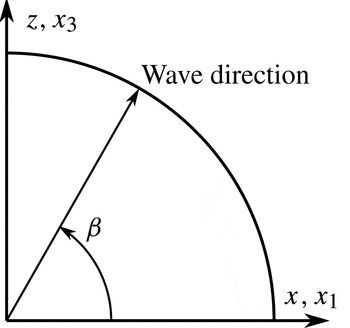
) in detail. We introduce the obliqueness angle
 ${\it\beta}$
as shown in figure 3. The angle
 ${\it\beta}$
is a measure of the obliqueness to the downstream direction on the
 $x_{1}{-}x_{3}$
plane. Now recognizing that
 $$\begin{eqnarray}{\it\kappa}_{1}(0)={\it\kappa}(0)\cos {\it\beta},\end{eqnarray}$$
we can write
 $$\begin{eqnarray}\displaystyle {\it\kappa}^{2}\! & = & \displaystyle \!{\it\kappa}_{1}^{2}(0)+{\it\kappa}_{2}^{2}(0)-2{\it\kappa}_{2}(0){\it\kappa}_{1}(0)St+{\it\kappa}_{1}^{2}(0)S^{2}t^{2}+{\it\kappa}_{3}^{2}(0)\nonumber\\ \displaystyle \! & = & \displaystyle \!{\it\kappa}_{0}^{2}(1+S^{2}t^{2}\cos ^{2}{\it\beta})-2{\it\kappa}_{2}(0){\it\kappa}(0)\cos {\it\beta}.\end{eqnarray}$$
Now (3.13) can be simplified as
 $$\begin{eqnarray}\frac{\text{d}^{3}\hat{p}}{\text{d}t^{3}}\approx -a_{0}^{2}{\it\kappa}_{0}^{2}\cos ^{2}({\it\beta})S^{2}\left(t^{2}\frac{\text{d}\hat{p}}{\text{d}t}+4t\hat{p}\right).\end{eqnarray}$$
Equation (3.17) suggests a critical scaling relationship. For oblique modes, the effective shear can be defined as
 $$\begin{eqnarray}S^{\ast }=S\cos ({\it\beta}),\end{eqnarray}$$
and the corresponding effective gradient Mach number experienced by an oblique mode is
 $$\begin{eqnarray}M_{g}^{\ast }\equiv \frac{S^{\ast }l}{a}=\frac{S^{\ast }}{a_{0}|{\it\kappa}(0)|}=M_{g0}\cos ({\it\beta}).\end{eqnarray}$$
Here
 $M_{g0}$
is the gradient Mach number experienced by a streamwise perturbation of length
 $l$
or wavenumber
 ${\it\kappa}_{0}=1/l$
. Now, defining non-dimensional time as
 $$\begin{eqnarray}t^{\ast }=(a_{0}{\it\kappa}_{0}S\cos ({\it\beta}))^{1/2}t,\end{eqnarray}$$
(3.17) can be written as
 $$\begin{eqnarray}\frac{\text{d}^{3}\hat{p}}{\text{d}t^{\ast 3}}=-\!\left(t^{\ast 2}\frac{\text{d}\hat{p}}{\text{d}t^{\ast }}+4t^{\ast }\hat{p}\right),\end{eqnarray}$$
where the non-dimensional time
 $t^{\ast }$
can be cast as
 $$\begin{eqnarray}t^{\ast }=\frac{S^{\ast }t}{\sqrt{M_{g0}^{\ast }}}.\end{eqnarray}$$
Self-similar (3.17) leads to several critical inferences:
-
(a) The main dimensionless parameter that characterizes the modal behaviour of pressure is
$M_{g}^{\ast }$
and not
${\it\beta}$
,
$M_{g}$
or
${\it\kappa}$
individually. The modal pressure behaviour is self-similar when considered in dimensionless time
$t^{\ast }$
. -
(b) Oblique modes are subject to decreasing effective Mach number with increasing angle:
$M_{g}^{\ast }=M_{g0}\cos ({\it\beta})$
. Streamwise modes (
${\it\beta}=0$
) experience the highest compressibility effect and spanwise modes (
${\it\beta}={\rm\pi}/2$
) the least. In fact, the effective Mach number of a spanwise mode is zero. Clearly,
$M_{g0}$
is the Mach number experienced by the streamwise mode (
${\it\beta}=0$
). This is the maximum effective Mach number in the flow and is called the reference Mach number. -
(c) Even in very high-speed flows, there exists a critical obliqueness angle,
(3.23)beyond which all modes experience subsonic Mach numbers. Clearly, the critical angle increases with increasing Mach number.
$$\begin{eqnarray}{\it\beta}_{crit}=\cos ^{-1}\left(\frac{1}{M_{g0}}\right),\end{eqnarray}$$





A typical oblique mode in modal simulations.
We will now examine the self-similar pressure behaviour. The pressure analysis is similar to that in Bertsch et al. (Reference Bertsch, Suman and Girimaji2012), but is extended to examine the behaviour of a single mode. The factor
 $$\begin{eqnarray}{\it\omega}_{0}^{4}\equiv (a_{0}{\it\kappa}_{1}(0))^{2}S^{2}=\frac{a_{0}^{2}{\it\kappa}_{1}^{2}(0)\cos ^{4}({\it\beta})S^{4}}{\cos ^{4}({\it\beta})S^{2}}=\frac{{S^{\ast }}^{4}}{{M_{g}^{\ast }}^{2}}\end{eqnarray}$$
on the right-hand side of (3.17) is proportional to the initial acoustic frequency (
 $a_{0}{\it\kappa}_{1}(0)$
) and effective shear (
 $S^{\ast }$
). With
 $q$
and
 $r$
defined as
 $q={\it\omega}_{0}^{4}t^{2}$
and
 $r=4{\it\omega}_{0}^{4}t$
, (3.17) is cast as
 $$\begin{eqnarray}\frac{\text{d}^{3}\hat{p}}{\text{d}t^{3}}+q\frac{\text{d}\hat{p}}{\text{d}t}+r\hat{p}\approx 0.\end{eqnarray}$$
Here
 $q$
and
 $r$
are the time-dependent coefficients of the third-order ordinary differential equation (ODE). At this point, the pressure analysis given in Bertsch et al. (Reference Bertsch, Suman and Girimaji2012) can be directly adapted.
Referring to Bertsch et al. (Reference Bertsch, Suman and Girimaji2012), the pressure evolution can be categorized into three stages: early, intermediate and late. The early stage occurs during the period (Bertsch et al. Reference Bertsch, Suman and Girimaji2012)
 $$\begin{eqnarray}\frac{St}{\sqrt{M_{g0}}}\approx 1.\end{eqnarray}$$
During this period, the pressure evolution exponents are given by
 $$\begin{eqnarray}y\approx {\it\omega}_{0}^{4/3}t^{1/3}.\end{eqnarray}$$
The onset of the late stage occurs after one acoustic time (Bertsch et al. Reference Bertsch, Suman and Girimaji2012),
 $$\begin{eqnarray}\frac{a_{0}t}{l_{0}}\gg 1\quad \text{or}\quad St>\frac{S\ell _{0}}{a_{0}}=M_{g0}.\end{eqnarray}$$
At this stage, the pressure exponent grows linearly in time:
 $$\begin{eqnarray}y\approx {\it\omega}_{0}^{2}t\approx (a_{0}{\it\kappa}(0))St.\end{eqnarray}$$
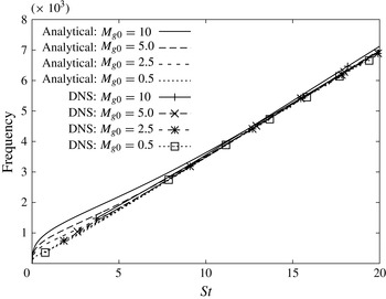
The last inequality comes from (3.24). This analytical result will be verified against DNS data in figure 6. Also, recall that
 $a_{0}\approx 350\ \text{m}\ \text{s}^{-1}$
in the simulations performed in this paper. The duration of the intermediate stage is between the limits given in (3.26) and (3.29).
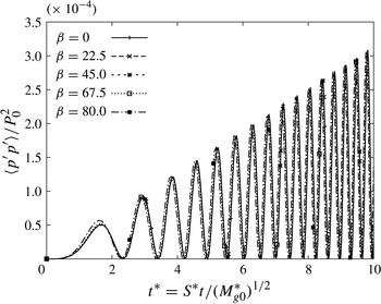
Scaling of amplitude and frequency of pressure in RDT for different
 ${\it\beta}$
in
 $t^{\ast }$
time. For all cases
 $|{\it\kappa}_{0}|$
and
 $S$
are identical. For
 ${\it\beta}=0$
and
 ${\it\kappa}_{0}=1$
, the Mach number is
 $M_{g0}=10$
.

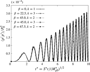
Scaling of amplitude and frequency of pressure in RDT for different
 ${\it\beta}$
in
 $t^{\ast }$
time. For all cases only
 $S$
is identical. For
 ${\it\beta}=0$
and
 ${\it\kappa}_{0}=1$
, the effective initial Mach number is
 $M_{g0}=10$
.

The main inferences of the pressure analysis are examined using DNS and RDT data in figures 4–6. In figure 4, the RDT pressure–variance evolution is shown for different obliqueness modes at a given reference Mach number
 $M_{g0}=10$
. The scaled variance evolutions of the different modes collapse on to a single line. Figure 5 shows a similar collapse of the RDT pressure variance evolution for different initial wavenumber magnitudes. The scaling is further verified with DNS data in figure 6. The analytical (3.29) and computed pressure–amplitude evolution frequencies are compared at different times. The DNS data clearly show the linear trend and the proposed scaling over a wide Mach number range. Referring to figure 6, frequency evolution is independent of Mach number in
 $St$
time units. It must be pointed out that
 $S$
is a strong function of Mach number. The dependence on
 $M_{g0}$
is hidden in the normalization of time,
 $St$
. The value of
 $S$
is different for different Mach numbers. The DNS frequency is obtained from averaging over three cycles of simulated evolution, whereas the theoretical estimate is obtained from the analytical approximation at a given instant. The theoretical linear scaling applies in the range
 $St>M_{g0}$
, (3.28). The apparent linear DNS behaviour seen in the figure at early times is due to the averaging process. In summary, the self-similar dependence of pressure on obliqueness and Mach number is clearly demonstrated.
Comparison of DNS and RDT analysis for frequency of pressure amplitude oscillations:
 $M_{g0}=0.5,2.5,5.0,10.0\ ({\it\beta}=0)$
. The slope is clearly
 $a_{0}\approx 350$
.

3.2. Modal behaviour of velocity and kinetic energy
Having established the characteristics of pressure fluctuation evolution, we will now examine the behaviour of velocity fluctuations as a function of obliqueness angle and Mach number. It is first useful to summarize the velocity perturbation behaviour when subject to Burgers and incompressible flow equations. The evolution of kinetic energy in Burgers turbulence is given in (2.22) and is clearly independent of the mode wavevector orientation,
 ${\it\beta}$
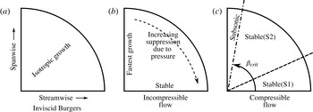
. In incompressible flow, pressure suppresses streamwise perturbations and does not affect spanwise modes (Mishra & Girimaji Reference Mishra and Girimaji2013). A schematic of these effects is presented in figure 7. The goal of this subsection is to understand how compressibility effects the stability of modal kinetic energy as a function of
 ${\it\beta}$
.
Schematics of modal stability in (a) Burgers, (b) incompressible and (c) compressible flows.

Equations (3.8) and (3.9) reveal the pivotal role played by the
 ${\hat{u}}_{2}$
component on perturbation evolution. The
 ${\hat{u}}_{2}$
behaviour in turn depends on
 $\hat{p}$
. The first step towards examining perturbation evolution is to characterize
 ${\hat{u}}_{2}$
evolution as a function of Mach number and
 ${\it\beta}$
. In the previous subsection, three categories of wavevector modes were identified. It was shown that case 2, wherein
 ${\it\kappa}_{2}(0)=0$
, is the most significant. This subsection also focuses on case 2 wavevectors. An autonomous equation for
 ${\hat{u}}_{2}$
can be obtained by differentiating (2.18) twice and following a procedure similar to that of the pressure equation (3.13):
 $$\begin{eqnarray}\displaystyle & & \displaystyle \displaystyle \frac{\text{d}^{2}{\hat{u}}_{2}}{\text{d}t^{2}}=-\frac{\text{i}}{\bar{{\it\rho}}}[-\text{i}{\it\gamma}\bar{p}{\hat{u}}_{j}{\it\kappa}_{j}{\it\kappa}_{2}-\hat{p}{\it\kappa}_{j}S_{j2}],\end{eqnarray}$$
 $$\begin{eqnarray}\displaystyle & & \displaystyle \displaystyle \frac{\text{d}^{3}{\hat{u}}_{2}}{\text{d}t^{3}}=-\frac{{\it\gamma}\bar{p}}{\bar{{\it\rho}}}\left[\frac{\text{d}{\hat{u}}_{2}}{\text{d}t}{\it\kappa}^{2}-4{\hat{u}}_{2}{\it\kappa}_{1}{\it\kappa}_{2}S-2({\hat{u}}_{1}{\it\kappa}_{1}+{\hat{u}}_{3}{\it\kappa}_{3}){\it\kappa}_{1}S\right]\!.\end{eqnarray}$$
 $({\hat{u}}_{1}{\it\kappa}_{1}+{\hat{u}}_{3}{\it\kappa}_{3})$
term in (3.31). Despite this difference, these equations clearly indicate a harmonic interaction between
 $\hat{p}$
and
 ${\hat{u}}_{2}$
. The implication is that there is equipartition between the kinetic energy (
 ${\it\rho}\overline{u_{2}u_{2}}$
) and potential energy (
 $\,\overline{p^{\prime }p^{\prime }}/{\it\gamma}\bar{{\it\rho}}$
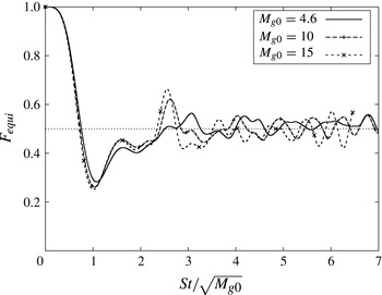
). For further details on equipartition, the reader is referred to Bertsch et al. (Reference Bertsch, Suman and Girimaji2012, equations (44)–(54)). To investigate this further, we define the equipartition parameter
 $$\begin{eqnarray}F_{equi}=\frac{\overline{p^{\prime }p^{\prime }}}{\overline{u_{2}^{\prime }u_{2}^{\prime }}\bar{p}\bar{{\it\rho}}{\it\gamma}}.\end{eqnarray}$$
The evolution of
 $F_{equi}$
for a collection of randomly distributed modes computed from DNS is shown in figure 8. Clearly, for a range of Mach numbers,
 $F_{equi}$
oscillates around a value of 0.5 after the initial transient period. Evidently,
 ${\hat{u}}_{2}$
is driven to oscillatory behaviour by the wave-like evolution of pressure.
Evolution of equipartition of pressure and dilatational kinetic energy in the streamwise mode
 $({\it\beta}=0)$
.

This compressible
 ${\hat{u}}_{2}$
behaviour must be contrasted with its character in incompressible flows. In incompressible shear flow,
 ${\hat{u}}_{2}$
evolves according to
 $$\begin{eqnarray}\frac{\text{d}{\hat{u}}_{2}}{\text{d}t}={\hat{u}}_{2}S\frac{{\it\kappa}_{1}{\it\kappa}_{2}}{{\it\kappa}^{2}}\approx -\frac{{\hat{u}}_{2}}{t},\end{eqnarray}$$
the final approximation being valid after the initial transients. Thus, at low Mach numbers,
 ${\hat{u}}_{2}$
decays in magnitude monotonically and its sign remains unchanged.
Now the nature of production at high and low Mach numbers can be contrasted. As
 $P\approx -\overline{u_{1}u_{2}}S$
, and the sign of shear is constant, it can be concluded that production will be oscillatory at high Mach number (Bertsch et al.
Reference Bertsch, Suman and Girimaji2012) and retain its sign at low Mach number. Given this background, we will now examine individual modes.
3.2.1. Spanwise modes (
${\it\beta}={\rm\pi}/2$
)

For this case,
 ${\it\kappa}_{1}(t)=0,{\it\kappa}_{2}(t)=0,{\it\kappa}_{3}(t)={\it\kappa}_{3}(0)=1$
. The velocity amplitude equations can be reduced to
 $$\begin{eqnarray}\displaystyle & & \displaystyle \displaystyle \frac{\text{d}{\hat{u}}_{1}}{\text{d}t}=-{\hat{u}}_{2}S,\end{eqnarray}$$
 $$\begin{eqnarray}\displaystyle & & \displaystyle \displaystyle \frac{\text{d}{\hat{u}}_{2}}{\text{d}t}=0,\end{eqnarray}$$
 $$\begin{eqnarray}\displaystyle & & \displaystyle \displaystyle \frac{\text{d}{\hat{u}}_{3}}{\text{d}t}=-\text{i}\frac{\hat{p}}{\bar{{\it\rho}}}.\end{eqnarray}$$
 $$\begin{eqnarray}(u,v,w)=(0,\sin (nz+{\it\Delta}),0),\end{eqnarray}$$
where
 $n\in [1,2,3,\dots ]$
is the wavenumber and
 ${\it\Delta}\in [0,{\rm\pi}]$
is an arbitrary phase shift. The velocity field is initially divergence-free with fluctuations along the direction of shear.
Owing to the fact that
 $\cos ({\rm\pi}/2)=0$
, both the incompressible and compressible contributions of the pressure vanish from the
 ${\hat{u}}_{1}$
and
 ${\hat{u}}_{2}$
equations. Even the
 ${\hat{u}}_{3}$
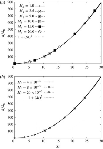
amplitude does not change significantly. In summary, the velocity amplitudes are entirely unaffected by pressure and evolve according to Burgers dynamics (production only) regardless of Mach number. Thus, the evolution of velocity components and kinetic energy of spanwise perturbation modes will be nearly identical to Burgers for both incompressible and compressible shear flows. The DNS evolution of kinetic energy of initial spanwise perturbation modes (
 ${\it\kappa}_{3}(0)=1$
) computed at various gradient Mach numbers is shown in figure 9(a). Independent of the Mach number, the energy evolution follows the analytical Burgers solution. In figure 9(b), the effect of initial velocity amplitudes is examined. Provided the initial turbulent Mach number
 $(M_{t0}=\sqrt{u_{i}^{\prime }u_{i}^{\prime }(0)}/a_{0})$
is small, the kinetic energy evolution again collapses to the Burgers expression.
DNS evolution of kinetic energy (
 $k/k_{0}$
) for the
 ${\it\beta}={\rm\pi}/2$
(spanwise) mode in shear time: (a) effect of initial modal gradient Mach number
 $M_{g0}$
and (b) effect of initial turbulent Mach number
 $M_{t0}$
.

3.2.2. Streamwise modes (
${\it\beta}=0$
)

As seen in the previous section, the streamwise modes experience the highest effective Mach number and thus are most influenced by compressibility. For this case,
 ${\it\kappa}_{1}(t)={\it\kappa}_{1}(0)=1,{\it\kappa}_{2}(t)=-{\it\kappa}_{1}(0)St=-St,{\it\kappa}_{3}(t)=0$
. The evolution equations of the various velocity amplitudes reduce to
 $$\begin{eqnarray}\displaystyle \displaystyle \frac{\text{d}{\hat{u}}_{1}}{\text{d}t} & = & \displaystyle \displaystyle -{\hat{u}}_{2}S-\text{i}\frac{\hat{p}}{\bar{{\it\rho}}}{\it\kappa}_{1},\end{eqnarray}$$
 $$\begin{eqnarray}\displaystyle \displaystyle \frac{\text{d}{\hat{u}}_{2}}{\text{d}t} & = & \displaystyle \displaystyle -\text{i}\frac{\hat{p}}{\bar{{\it\rho}}}{\it\kappa}_{2},\end{eqnarray}$$
 $$\begin{eqnarray}\displaystyle \displaystyle \frac{\text{d}{\hat{u}}_{3}}{\text{d}t} & = & \displaystyle 0,\end{eqnarray}$$
 $$\begin{eqnarray}\displaystyle \displaystyle \frac{\text{d}\widehat{p}}{\text{d}t} & = & \displaystyle \displaystyle -\text{i}{\it\gamma}\bar{p}(\hat{u_{1}}{\it\kappa}_{1}+\hat{u_{2}}{\it\kappa}_{2}).\end{eqnarray}$$
 $$\begin{eqnarray}(u,v,w)=(0,\sin (nx+{\it\Delta}),0),\end{eqnarray}$$
where
 $n\in [1,2,3,\dots ]$
is the wavenumber and
 ${\it\Delta}\in [0,{\rm\pi}]$
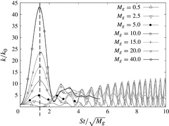
is an arbitrary phase shift. This velocity field is initially divergence-free with fluctuations along the direction of shear. The kinetic energy evolution of these streamwise modes is displayed in isolation on figure 10. Considering the streamwise mode does not grow in incompressible flow (Mishra & Girimaji Reference Mishra and Girimaji2013), it can be concluded that the observed behaviour is entirely due to dilatational fluctuations. It is important to note the similarity between kinetic energy evolution in figure 10 and the pressure–variance oscillations in figures 4 and 5, further confirming the harmonic oscillator paradigm. The oscillations also indicate the changing sign of production.
Effect of initial gradient Mach number (
 $M_{g0}$
) on streamwise mode
 $({\it\beta}=0)$
in normalized time. The vertical dashed line connects the peak of all
 $M_{g0}$
simulations at
 $St/M_{g0}\approx 1.4$
, in agreement with (3.26).

At earlier times, prior to the onset of harmonic behaviour, the kinetic energy follows Burgers evolution. With increasing initial modal gradient Mach number
 $M_{g0}$
, the evolution of kinetic energy follows Burgers evolution for a longer duration (
 $St\approx \sqrt{M_{g0}}$
). Prior to this time, the pressure field exerts no influence on the velocity field (see (3.26)). Eventually, kinetic energy evolution for all
 $M_{g0}$
departs from Burgers when the pressure effect becomes comparable to shear or, equivalently, the pressure time scale decreases to become comparable to the shear time scale.
3.2.3. Evolution of supersonic oblique modes:
${\it\beta}\in (0,{\it\beta}_{crit})$

Oblique modes combine characteristics of both spanwise and streamwise modes. The initial conditions for the fluctuating velocity field are given by
 $$\begin{eqnarray}\boldsymbol{u}\equiv (u,v,w)=(0,\sin (mx+nz+{\it\Delta}),0),\quad {\it\Delta}\in [0,{\rm\pi}],\end{eqnarray}$$
where
 $m$
and
 $n$
are wavenumbers and
 ${\it\Delta}$
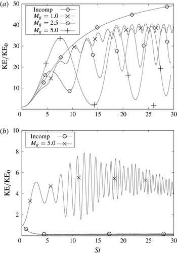
is an arbitrary phase shift. In figure 11, we present the kinetic energy evolution of different oblique modes at various Mach numbers.
Growth of kinetic energy for oblique modes: (a)
 ${\it\beta}=78.69^{\circ }$
, (b)
 ${\it\beta}=11.31^{\circ }$
.

Evolution of kinetic energy for oblique modes with larger spanwise component (
 ${\it\kappa}_{3}>{\it\kappa}_{1}$
) is shown in figure 11(a). We see that at initial times all modes grow like Burgers, which is consistent with the initial time behaviour of both the
 ${\it\beta}=0$
and
 ${\it\beta}={\rm\pi}/2$
modes. Oblique modes with higher
 $M_{g0}$
follow Burgers growth for a longer time and have larger kinetic energy. Eventually, all modes depart from Burgers trajectory and show an oscillatory evolution of kinetic energy, which is characteristic of the
 ${\it\beta}=0$
mode. With increasing
 $M_{g0}$
, the amplitude of temporal oscillations increases as the time period decreases. At late shear times, the overall growth (averaged over an oscillation) shows an inverse relationship with
 $M_{g0}$
and eventually becomes lower than incompressible evolution. Therefore, oblique modes with larger spanwise component (large
 ${\it\beta}$
) have lower mean kinetic energy than their incompressible counterparts. We characterize this region as S2. For wavevectors in this region, the asymptotic kinetic energy decreases with Mach number in the linear regime of development.
Evolution of kinetic energy for oblique modes with larger streamwise component (
 ${\it\kappa}_{1}>{\it\kappa}_{3}$
, small
 ${\it\beta}$
) is shown in figure 11(b). In incompressible or low-
 $M_{g0}$
flows, streamwise modes (
 ${\it\beta}=0$
) decay in time. With increase in
 $M_{g0}$
, the growth in kinetic energy increases. All oblique modes with high enough gradient Mach number
 $M_{g0}>1$
follow Burgers trajectory at early times. All oblique modes eventually depart from Burgers evolution and show an oscillatory evolution of kinetic energy typical of streamwise modes. Therefore, kinetic energy of oblique modes with higher streamwise component (small
 ${\it\beta}$
) increases with increasing
 $M_{g0}$
, but they are still stable at late times. We identify this region of
 ${\it\beta}$
as S1. For S1 wavevectors, the asymptotic kinetic energy increases with Mach number.
Evolution of kinetic energy for oblique modes around
 ${\it\beta}_{crit}$
: (a)
 $M_{g0}=5$
and (b)
 $M_{g0}=10$
.

The simulation results lead to the following inferences. With increasing effect of compressibility (or increasing
 $M_{g0}$
), the behaviour of the oblique mode is dependent on the ratio of spanwise to streamwise component in the mode. When the streamwise component is higher, increasing compressibility has a transient growth effect. When the spanwise component is higher, increasing
 $M_{g0}$
has a stabilizing effect. We observe that the overall kinetic energy associated with oblique modes having higher spanwise component is significantly higher (
 ${\sim}5$
times) than its counterpart of larger streamwise component.
3.2.4. Evolution of subsonic oblique modes:
${\it\beta}>{\it\beta}_{crit}$

Now we examine the importance of the critical angle (
 ${\it\beta}_{crit}$
). Recall that
 ${\it\beta}_{crit}$
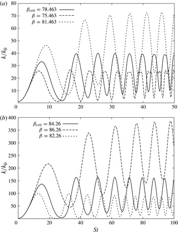
demarcates modes experiencing subsonic and supersonic effects. In figure 12, we show growth of kinetic energy for oblique modes around
 ${\it\beta}_{crit}$
for
 $M_{g0}=5$
and 10. For
 $M_{g0}=5$
and 10,
 ${\it\beta}_{crit}$
is 78.463 and 84.26°, respectively. At both Mach numbers, the subsonic modes show a clear growth trend whereas the supersonic modes exhibit slow but discernible decay. The critical mode appears to be neutrally stable. Thus it is evident that the critical angle not only demarcates subsonic and supersonic modes, but also marks the boundary between stable and growing perturbations. At times longer than the duration shown in figure 12, the nonlinear effects set in. Comparison of DNS against linear analysis will be invalid beyond this time.
3.2.5. On the period of validity of linear analysis
To establish the period of validity of the linear analysis, we examine the various time scales of relevance. There are three important time scales to consider when investigating shear flows, namely, shear, viscous and perturbation:
 $$\begin{eqnarray}\displaystyle {\it\tau}_{S} & = & \displaystyle \displaystyle \frac{1}{S},\end{eqnarray}$$
 $$\begin{eqnarray}\displaystyle {\it\tau}_{{\it\nu}} & = & \displaystyle \displaystyle \frac{1}{{\it\nu}{\it\kappa}^{2}}\approx \frac{1}{{\it\nu}{\it\kappa}_{0}^{2}\cos ^{2}({\it\beta})S^{2}t^{2}},\end{eqnarray}$$
 $$\begin{eqnarray}\displaystyle {\it\tau}_{p} & = & \displaystyle \displaystyle \frac{1}{{\hat{u}}{\it\kappa}}\approx \frac{1}{{\hat{u}}{\it\kappa}_{0}\cos ({\it\beta})St}.\end{eqnarray}$$
 $$\begin{eqnarray}{\it\tau}_{S}<{\it\tau}_{{\it\nu}}\quad \text{and}\quad {\it\tau}_{S}<{\it\tau}_{p},\end{eqnarray}$$
or more succinctly
 $$\begin{eqnarray}S>{\it\nu}{\it\kappa}^{2}\quad \text{and}\quad S>{\hat{u}}{\it\kappa}.\end{eqnarray}$$
The requirement that the shear time scale be smaller than the viscous time scale leads to the following inequality:
 $$\begin{eqnarray}St<\frac{\sqrt{M_{g0}}\sqrt{\mathit{Re }_{a}}}{\cos {\it\beta}}\quad \text{where }\mathit{Re}_{a}=\frac{a_{0}}{{\it\nu}{\it\kappa}_{0}}.\end{eqnarray}$$
The value of viscosity used in these runs is several orders of magnitude smaller than the speed of sound (
 $a_{0}\approx 3.47\times 10^{2}\ \text{m}\ \text{s}^{-1};{\it\nu}\approx 10^{-4}$
), resulting in very large
 $\mathit{Re}_{a}$
. For this reason, the first requirement (3.49) is satisfied for a significant period of time. The other requirement wherein the shear time scale must be smaller than the perturbation time scale leads to
 $$\begin{eqnarray}St<\frac{M_{g0}}{M_{t}}\frac{1}{\cos {\it\beta}}\quad \text{where }M_{t}=\frac{\sqrt{k}}{a_{0}}.\end{eqnarray}$$
The magnitude of the velocity perturbation is typically several orders smaller than the mean shear magnitude. Therefore, the turbulent Mach number (
 $M_{t}$
) is much smaller than the gradient Mach number. For individual perturbation modes, the validity of the linear inviscid analysis is dependent on the wave mode orientation. For spanwise modes, larger
 ${\it\beta}$
, (3.49) and (3.50) are satisfied for a very long period of time, so linear inviscid analysis can be used for longer simulations. For the streamwise mode,
 ${\it\beta}\approx 0$
, linear inviscid analysis is only valid until
 $$\begin{eqnarray}St<\sqrt{M_{g0}}\sqrt{\mathit{Re }_{a}}\quad \text{and}\quad St<\frac{M_{g0}}{M_{t}}.\end{eqnarray}$$
It is important to note that
 $M_{t}$
evolves in time, whereas
 $M_{g0}$
represents the initial value.
3.2.6. Summary
Based on these findings, we can now present the effect of compressibility on perturbation mode stability in shear flows (figure 7). In compressible shear flows, the
 ${\it\beta}$
plane can be divided into three parts. The subsonic modes (
 ${\it\beta}>{\it\beta}_{crit}$
) exhibit kinetic energy growth, but the rate is smaller than that of their incompressible counterparts. Here
 ${\it\beta}_{crit}$
increases with increasing Mach number. All supersonic modes appear to be stable, but can be subdivided into two categories: S1 and S2. As seen from linear analysis, closer proximity to the shear plane leads to a stronger compressibility effect. Therefore, lower values of
 ${\it\beta}$
experience larger dilatational fluctuations. On the other hand, solenoidal fluctuations become weaker at low
 ${\it\beta}$
values. Thus, there exists a range of modes (S1 region) wherein the dilatational component of the velocity field is stronger than the solenoidal part. In this range of modes, the kinetic energy will increase with higher Mach number. Correspondingly, there exists a second regime of
 ${\it\beta}$
values (S2 region) wherein the solenoidal energy is dominant. However, the growth of solenoidal energy diminishes with Mach number owing to the oscillatory effect of dilatational fluctuations. In this S2 regime, kinetic energy diminishes with increasing Mach number. The transition between the S1 and S2 regimes is gradual and will be investigated in future works.
4. Role of obliqueness in stabilization
We now attempt to consolidate the results in the previous sections to provide a complete explanation of the stabilizing action of pressure in shear flows. Specifically, we seek to explicate the role of perturbation obliqueness in the three-stage kinetic energy evolution observed in previous studies of a collection of perturbation modes (Bertsch et al. Reference Bertsch, Suman and Girimaji2012; Lavin et al. Reference Lavin, Girimaji, Suman and Yu2012). Bertsch et al. (Reference Bertsch, Suman and Girimaji2012) characterize the three regimes as follows. In the early-time regime, the kinetic energy evolves as in Burgers turbulence exclusively due to production. In this regime, the kinetic energy in compressible turbulence grows more rapidly than its incompressible counterpart. In the second intermediate-time regime, the kinetic energy growth comes to a near halt. During this period, the incompressible shear flow kinetic energy surpasses that of compressible flows. Here, pressure counteracts the production of shear stress, leading to near zero growth in kinetic energy. The stabilizing effect of compressibility is most evident in this regime. In the final regime, kinetic energy grows again but the energy level lags well behind that in incompressible flow at the same normalized lapse time. All the above results pertain to the statistical average of several modes. We will now explain the collective behaviour from that of individual mode kinetic energy evolution.
(a) Evolution of turbulent kinetic energy for a collection of perturbations subject to a range of initial gradient Mach numbers,
 $M_{go0}$
. (b) Evolution of kinetic energy for two gradient Mach numbers and various initial
 $\mathit{Re}_{{\it\lambda}}$
.

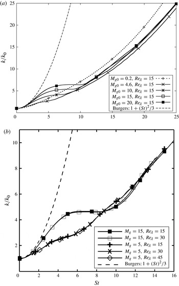
First, we present the kinetic energy evolution from several high-Mach-number collective-mode homogeneous shear flow DNS cases in figure 13(a). The initial Mach numbers in the simulations cover a wide range:
 $M_{g0}=0.2$
to
 $M_{g0}=20$
. For all the cases, the initial spectrum is given by (2.23). The initial
 $\mathit{Re}_{{\it\lambda}}$
for all cases is 15. The Reynolds number increases to much larger values with the evolution of kinetic energy. The low-speed case (
 $M_{g0}=0.2$
) shows a near-monotonic growth in the kinetic energy. The supersonic cases, however, exhibit a distinct three-stage evolution. Figure 13(b) displays the evolution of kinetic energy for a range of initial
 $\mathit{Re}_{{\it\lambda}}$
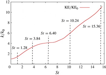
for two distinct initial Mach numbers. At the higher Reynolds numbers, the nonlinear interactions between the fluctuations become more important, even at the initial stages, as indicated by the ratio of the mean to perturbation strain rate. Nevertheless, as shown in figure 13(b), the advent of nonlinear interactions has only very little influence on the qualitative aspects of kinetic energy evolution. To better understand the physics of the different stages, we will focus our attention on one case given in figure 14:
 $M_{g0}=10$
. We now analyse the modal content of energy at various times encompassing the three stages or regimes. At any given time, the energy of all modes with a given value of
 $({\it\kappa}_{1},{\it\kappa}_{3})$
is calculated as follows:
 $$\begin{eqnarray}E({\it\kappa}_{1},{\it\kappa}_{3})\equiv \frac{1}{2}\mathop{\sum }\limits_{{\it\kappa}_{2}}{\hat{u}}({\it\kappa}_{1},{\it\kappa}_{2},{\it\kappa}_{3})\,{\hat{u}}^{\ast }({\it\kappa}_{1},{\it\kappa}_{2},{\it\kappa}_{3}).\end{eqnarray}$$
The sampling times are marked in figure 14:
 $St=0.0$
(random, isotropic velocity field at
 $t=0$
),
 $St=1.28$
(in stage 1),
 $St=3.84$
(beginning of stage 2),
 $St=6.40$
(in stage 2),
 $St=10.24$
(early stage 3) and
 $St=15.36$
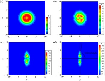
(late stage 3). The energy content as a function of
 $({\it\kappa}_{1},{\it\kappa}_{3})$
is shown in figure 15 in the form of contour plots. The contour plots are only shown for the first four times indicated above. The subsequent distributions are restricted to a very narrow band near the
 $x_{3}$
axis. The role of perturbation obliqueness emerges from figures 7, 14 and 15.
Kinetic energy evolution for collection of modes for
 $M_{g0}=10$
and
 $\mathit{Re}_{{\it\lambda}}=15$
.

Amplitude growth rate for different wavevectors: (a)
 $St=0.0$
, (b)
 $St=1.28$
, (c)
 $St=3.84$
and (d)
 $St=6.4$
.

Early times. The DNS starts from an isotropically distributed perturbation field, and consequently the energy distribution is also isotropic as shown in figure 15(a). At early times, the pressure effect is negligible and all modes grow equally. Thus energy distribution among the modes continues to be isotropic as seen in figure 15(b). At low Mach numbers, pressure acts instantly to curb all streamwise perturbations as shown in figure 7(b). In compressible flows, the streamwise perturbations flourish during this period, making compressible flows more energetic. The overall growth rate at this stage is higher than in a comparable incompressible case owing to the absence of pressure action.
Intermediate times. At about
 $St=\sqrt{Mg_{0}}$
, pressure effects begin to manifest and suppress the velocity field evolution as explained in previous sections. The stabilization onset is earliest for the streamwise mode and progresses to higher levels of obliqueness. The migration of suppression from
 ${\it\beta}=0$
to higher obliqueness can be seen by comparing figure 15(c) and (d). Over the duration of the intermediate regime, all supersonic modes are gradually suppressed. During this period, the oblique supersonic modes are less energetic than their counterparts in incompressible flows. Thus, the incompressible case will be collectively more energetic than the compressible shear turbulence.
Final stage. In this stage, only the spanwise or very highly oblique subsonic modes survive. As has been established before, these modes are unaffected by pressure or compressibility effects. Thus, the collective energy grows again, arguably at a rate similar to that in incompressible flows. Recall that, even in incompressible flows, these spanwise modes are dominant as shown in Mishra & Girimaji (Reference Mishra and Girimaji2013). Although the compressible and incompressible cases may have similar kinetic energy growth rates at this stage, the energy level of the latter will be higher than that of the former owing to the advantage gained in the intermediate regime.
5. Conclusions
The main objective of the present work is to examine the effect of perturbation obliqueness and Mach number on the stability of high-speed shear flows. Towards this end, linear analysis of the governing equations is performed and the outcome is verified against DNS data. The main findings are now summarized:
-
(1) The evolution of pressure amplitude of a given perturbation mode is self-similar over a range of obliqueness angles and Mach numbers when scaled as shown in (3.19) and (3.20).
-
(2) Pressure significantly influences the evolution of streamwise modes while the spanwise modes are relatively unaffected.
-
(3) The evolution of velocity perturbation amplitude depends strongly on obliqueness angle and Mach number. The obliqueness space can be demarcated into three regions as shown in figure 7. The demarcation between the three regions depends upon Mach number as given in (3.23). The modes in the subsonic region behave nearly similar to their counterparts in incompressible flow and exhibit linear growth. The supersonic modes (see figure 12) can be further subdivided into two parts. Modes that are oriented predominantly along the streamwise direction (region S1 in figure 7) exhibit increasing kinetic energy at higher Mach numbers, but are asymptotically stable. Supersonic modes oriented closer towards the spanwise direction become less energetic with increasing Mach number and are linearly stable (region S2).
The findings of the paper describe the vital role of perturbation obliqueness on shear flow instability in homogeneous compressible flows. In future works, the effects of the Kelvin–Helmholtz instability (mixing layers) and the Tollmien–Schlichting instability (boundary layers) will also be included.