1. Introduction
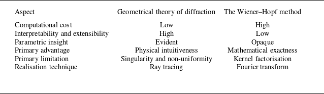
The issue of sound diffracted by an unflanged, semi-infinite duct is a classic and fascinating topic of acoustics. The exact analytical solution to this problem is available by the Wiener–Hopf method, which was introduced by Levine & Schwinger (Reference Levine and Schwinger1948) for the determination of radiation and reflection properties of plane acoustic waves from circular duct terminations in quiescent media. Generalisations that apply to modal waves can be found in the works of Weinstein (Reference Weinstein1969), Homicz & Lordi (Reference Homicz and Lordi1975), Savkar (Reference Savkar1975), Munt (Reference Munt1977), Rienstra (Reference Rienstra1984), Gabard & Astley (Reference Gabard and Astley2006) and Veitch & Peake (Reference Veitch and Peake2008), amongst others. However, given the lack of physical interpretability inherent in the Wiener–Hopf technique (Carrier Reference Carrier1959), simpler asymptotic approximations have been found to be more practical for analysing the noise produced by turbofan engines (Chapman Reference Chapman1994).
Chapman (Reference Chapman1994) has proposed the geometrical theory of diffraction (GTD), developed by Keller (Reference Keller1957, Reference Keller1958, Reference Keller1962), as a powerful asymptotic method for analysing the acoustics of circular ducts. The GTD has the advantage of being physically intuitive by explicitly revealing the diffracted rays’ trajectories and amplitudes. Through asymptotic analysis, Chapman (Reference Chapman1994) came up with the ingenious ray picture idea for duct modes in quiescent media and argued that, near the duct’s shroud, the modal waves are piecewise linear helices that produce a cone of diffracted rays when they strike the rim of the duct end. The semiangle
 $\beta _{K} = \cos ^{-1}{[m/(k a)]}$
of the cone is determined from the perspective of the ray geometry and the phase velocity, where
 $k a := \omega a/c_{0}$
is the duct Helmholtz number and
 $m$
is the azimuthal order of the mode.
Following up on Chapman’s (Reference Chapman1994) preliminary work, Hocter (Reference Hocter2000) advanced that the angle of incidence,
 $\varphi _{\!I}$
, and the distance from the edge to the other caustic of the diffracted rays,
 $\rho _{1}$
, should be
 $\varphi _{\!I} = \varphi _{\!I} (j'_{m,n}/k a)$
and
 $\rho _{1} \propto \sin ^{2}{\beta _{K}}$
, respectively, for determination of the radiated field from unflanged ducts in quiescent media. Instead, Keith & Peake (Reference Keith and Peake2002) proposed that
 $\varphi _{\!I} = \varphi _{\!I} (j'_{m,n}/k a, \beta _{K})$
and
 $\rho _{1} \propto \sin {\beta _{K}}$
for the same problem. Here,
 $j'_{m,n}$
denotes the eigenvalue of the
 $ (m, n )$
mode, details of which will be given in the following section. There were unresolved singularities in the fore and aft arcs in Hocter’s (Reference Hocter2000) and Keith & Peake’s (Reference Keith and Peake2002) solutions. The same radiation problem had previously been treated by Shirai & Felsen (Reference Shirai and Felsen1987), also on the basis of the GTD. By assuming the plane-wave nature of the incident and diffracted rays and by establishing a relationship between their wavenumber vectors, they obtained an asymptotic approximation for the forward radiated field. Their result takes an explicit dependence on
 $\beta _{K}$
in terms of magnitude. This dependency is evident in Keith & Peake’s (Reference Keith and Peake2002) results, but not in Hocter’s (Reference Hocter2000). The ambiguities in the treatment of the same diffraction problem arise, in part, from the difficulty of determining the GTD inputs associated with incident modal waves that are not capable of being approximated as plane waves.
In addition to radiating acoustic waves outwards, the duct termination also reflects them inwards through diffraction. The only publication that we are aware of that used the GTD to solve the reflection of modal waves from the openings of unflanged ducts was that of Felsen & Yee (Reference Felsen and Yee1968). Their analyses were restricted to modes with azimuthal order
 $m \in \{0, 1\}$
. Moreover, by incorporating inaccurate results from the parallel-plane analysis into their consideration (cf. Bowman Reference Bowman1970; Boersma Reference Boersma1975), the GTD-derived reflection coefficients seldom coincide with Levine & Schwinger’s (Reference Levine and Schwinger1948) Wiener–Hopf solution.
The issues concerning radiation and reflection that came before are about unflanged ducts. For open-ended ducts with flanges, the diffraction problem cannot be solved exactly by the Wiener–Hopf technique even in the absence of flow, for which the Wiener–Hopf functional equation involves three unknowns and the standard analytic continuation arguments are not immediately applicable (Noble Reference Noble1958, Chapter 5). By contrast, both unflanged and flanged geometries are accommodated within the GTD framework, and it is therefore anticipated that the asymptotic quality of results for the former is comparable to that for the latter (Yee, Felsen & Keller Reference Yee, Felsen and Keller1968; Felsen & Yee Reference Felsen and Yee1968). In the literature, possibly only Felsen & Yee (Reference Felsen and Yee1968) have extended the GTD solution to the case of flanged circular ducts, albeit with inaccurate approximations being adopted for lower-azimuthal-order modes, as previously stated, and in the context of the reflection problem. The more common analytical approach to solving the complete diffraction problem (radiation plus reflection) for flanged ducts is to numerically solve a linear system, which is derived on the basis of the Rayleigh diffraction integral, the continuity condition at the duct opening and the orthogonality of duct modes. A review of this topic can be found in Dokumacı’s (Reference Dokumacı2021, § 9) monograph. This method necessitates a truncated analysis of the linear system and still suffers from the drawback of lacking straightforward physical interpretability.
In their seminal work on the analysis of a plane wave diffraction by duct terminations, Levine & Schwinger (Reference Levine and Schwinger1948) simultaneously addressed the reciprocal problem of an external plane wave scattering by the unflanged duct via the reciprocity principle of the Helmholtz equation. The reciprocity relation establishes the connection between the radiation of an in-duct plane wave and the excitation of an in-duct plane wave induced by an external plane wave. An alternative method for obtaining Levine & Schwinger’s (Reference Levine and Schwinger1948) reciprocity relation involves directly employing the Wiener–Hopf method to derive solutions for both problems (Noble Reference Noble1958, § 3.4). Jones (Reference Jones1989, § 9.14) later broadened the reciprocity relation to include other non-spinning (
 $m \equiv 0$
) modes. In the case of full illumination, Shirai & Felsen (Reference Shirai and Felsen1987) had used the GTD to calculate the modal waves excited within the duct, based on the plane wave approximation of modal waves. The results of the GTD and the physical acoustics approximation were compared, and only at sufficiently high Helmholtz numbers (
 $k a = 100$
, say) were there slight discrepancies. Cho (Reference Cho1980a
) has thoroughly studied the reciprocity relations for duct acoustics. He did so by expanding the acoustic field, both interior and exterior to the duct, into duct modes and spherical harmonics, respectively, and by utilising their orthogonality properties in the application of the reciprocity principle. If the duct has a flange, Cho’s (Reference Cho1980a
) results are no longer applicable because the flange disrupts the orthogonality of the spherical harmonics. The reciprocal relation for flanged ducts in two dimensions has been established by Kriegsmann (Reference Kriegsmann1999), but no reports have yet been found for three dimensions.
We are aware that finding asymptotic approximations for the split functions of the Wiener–Hopf kernel, such as by expressing them in terms of Weinstein’s (Reference Weinstein1969) universal function, is one approach to simplifying the complex Wiener–Hopf solutions. Whilst this technique has been implemented for comparisons between the asymptotic approximations of the Wiener–Hopf and ray solutions for electromagnetic scattering problems (Bowman Reference Bowman1970), to the best of our knowledge, no comparison study has been done for acoustic waves yet. Such a comparison aims to furnish a reliable method for verifying the efficacy of proposed GTD techniques and their solutions, thereby establishing a basis for analysing more intricate configurations within the GTD framework, particularly those that are not amenable to direct solution via the Wiener–Hopf method.
Keller’s (Reference Keller1957, Reference Keller1958, Reference Keller1962) GTD, and any extensions to it, have hitherto only been applied to diffraction scenarios in the absence of medium flows. Given that the GTD was developed to solve the Helmholtz equation asymptotically, it is inherently incapable of providing analytical support for acoustics involving background medium flows. In the case of uniform medium flow, one viable approach is to employ the Prandtl–Glauert transformation to convert the GTD solution into the form of the asymptotic solution to the convected Helmholtz equation. However, when uniform flow is present, vortex shedding occurs at the trailing edge (Rienstra Reference Rienstra1981, Reference Rienstra1984). The GTD, in conjunction with the Prandtl–Glauert transformation, cannot account for the Kutta condition. Rarely is there any exploration on this topic.
This paper presents a systematic GTD procedure for addressing edge diffraction issues in duct acoustics in a manner that comprehensively furnishes insight into the underlying processes. The objective of our asymptotic study is to overcome the highlighted limitations of the referenced research and to elucidate the connection between the Wiener–Hopf and GTD solutions. We shall begin by addressing the diffraction issues associated with unflanged ducts, before generalising the analysis to flanged ducts. The trajectories and amplitudes of possible diffracted rays will be determined entirely within the framework of the GTD. These rays accumulate to produce the overall diffracted field. The GTD solutions will be compared with the Wiener–Hopf solutions, their steepest-descent approximations and experimental data for unflanged ducts. Numerical solutions for flanged ducts will also be used for comparison. We will extend Levine & Schwinger’s (Reference Levine and Schwinger1948) reciprocity relation to general cases by making use of the reciprocity principle and the method of stationary phase. In order to account for the Kutta condition, we will extend the GTD formulation by appealing to the canonical solution for the diffraction of a plane wave by a half-plane in the presence of a uniform flow. Beyond that, we will introduce a parameter to control the rate at which vortices are shed, as suggested in the Wiener–Hopf studies of Rienstra (Reference Rienstra1984) and Gabard & Astley (Reference Gabard and Astley2006).
None of our intentions, however, are feasible without first developing an asymptotic ray description of the modal wave to identify the legitimate inputs for the application of the GTD. Since acoustic rays propagate in the direction of the energy propagation velocity (Ostashev & Wilson Reference Ostashev and Wilson2015, § 3.3), we propose determining the incident angle
 $\varphi _{\!I}$
and the semiangle
 $\beta _{K}$
of the Keller cone for diffracted rays necessary for the GTD input by establishing the energy propagation angle of the incident ray. In modern turbofan engines, the blade and vane counts are typically very high, often around
 $20$
and
 $40$
, respectively. This leads to the generation of acoustic modes with a large azimuthal order
 $m$
, according to the rule of Tyler & Sofrin (Reference Tyler and Sofrin1962). Higher azimuthal-order modes are therefore indeed a common and dominant feature in turbofan noise prediction, and will therefore be the starting point of our asymptotic analysis. We should note that the large-
 $m$
requirement is employed solely to obtain an asymptotic approximation. As will be evidenced later, excellent approximations can still be achieved for sufficiently small
 $m$
; say,
 $m = 0$
.
The remainder of this article is arranged as follows. In § 2 we study exact and asymptotic solutions to the acoustic field in circular ducts, which are demanded for subsequent manipulations. Sections 3 and 4 determines the edge diffraction of in-duct modal waves by unflanged duct terminations. The extension of GTD solutions from unflanged to flanged ducts is provided in § 5. In § 6, the reciprocity relation between absorption and emission of the duct is deduced. Section 7 is devoted to correcting the GTD formulation to accommodate the Kutta condition. The paper concludes with § 8, which outlines several variants and extensions of the current work.
Notation. The subscript ‘
 $0$
’ denotes thermodynamic and kinetic variables of the steady background flow, while the prime ‘
 $'$
’ denotes perturbations associated with acoustic waves. (For functions such as Bessel or Airy functions, the prime retains its conventional meaning of differentiation.) The temporal Fourier transform is indicated by a hat,
 $\hat { (\boldsymbol{\cdot })}$
, and its subsequent Prandtl–Glauert transform by a check,
 $\check { (\boldsymbol{\cdot })}$
. Spatial and temporal coordinates in the transformed Prandtl–Glauert spacetime are marked with an overbar
 $\bar { (\boldsymbol{\cdot })}$
. Finally, the subscripts ‘
 $I$
’, ‘
 $R$
’ and ‘
 $D$
’ identify the incident, reflected and diffracted wave components, respectively.
2. In-duct acoustic field
We consider the case of a duct of uniform cylindrical cross-section of radius
 $a$
, carrying a homogeneous and moving medium at Mach number
 $- 1 \lt {M}_{0} \lt 1$
(
 $M_{0} \lt 0$
for intake and
 $M_{0} \gt 0$
for exhaust), with the axis aligned along the
 $z$
-axis, extending to
 $z = - \infty$
but terminating at
 $z = 0$
. The sketch of the duct and duct-fixed coordinates are shown in figure 1. The flow may be assumed homentropic potential, and the wave equation and the boundary condition for acoustic disturbances propagating in the case of rigid-walled ducts are
 \begin{equation} \left (\frac {1}{c_{0}^{2}} \frac {\mathrm{D}_{0}^{2} }{\mathrm{D} t^{2}} - {\nabla} ^{2} \right ) \phi ' = 0, \end{equation}
and
 $\left .(\partial \phi '/\partial r) \right |_{r = a } = 0$
, where
 $\mathrm{D}_{0}/\mathrm{D} t = \partial /\partial t + \boldsymbol{u}_{0} \boldsymbol{\cdot }\boldsymbol{\nabla}$
denotes the time derivative following the medium flow,
 $\boldsymbol{u}_{0} = c_{0} M_{0} \boldsymbol{e}_{z}$
,
 $\phi '$
the acoustic velocity potential and
 $c_{0}$
the sonic speed in the absence of acoustic disturbances.
Semi-infinite unflanged rigid-walled duct of radius
 $a$
immersed in an ambient flow of Mach number
 $M_{0} \boldsymbol{e}_{z}$
. In accordance with the geometry employed by Levine & Schwinger (Reference Levine and Schwinger1948), Noble (Reference Noble1958) and Rienstra (Reference Rienstra1984) for the purpose of comparing analytical solutions, the duct opening is situated at
 $z = 0$
, and the duct extends into the region
 $z \lt 0$
. The location of the observer can be anywhere in space. The geometric parameters
 $R$
,
 $\theta$
and
 $\varphi$
denote the radial distance, azimuthal angle and polar angle, respectively, in the spherical coordinate system.

Using
 $\boldsymbol{u}' = \boldsymbol{\nabla }\phi '$
and linearising the momentum equation in Crocco’s form (
 $\partial \boldsymbol{u}/\partial t + \boldsymbol{\nabla }\!B = \boldsymbol{0} \Rightarrow \partial \boldsymbol{\nabla }\phi '/\partial t = - \boldsymbol{\nabla }\!B'$
) and the energy equation (
 $\partial p/\partial t = \rho \mathrm{D} B/\mathrm{D} t \Rightarrow \partial p'/\partial t = \rho _{0} \mathrm{D}_{0} B'/\mathrm{D} t$
), and then eliminating the perturbation Bernoulli function
 $B'$
from the linearised equations, shows that, in the linear acoustics approximation, the acoustic pressure is given by
 \begin{equation} p' = - \rho _{0} \frac {\mathrm{D}_{0} \phi ' }{\mathrm{D} t}, \end{equation}
where
 $\rho$
is the density. In the linearisation, the relation
 $\partial \boldsymbol{u}_{0}/\partial t = \boldsymbol{0} \Leftrightarrow \boldsymbol{\nabla }\!B_{0} = \boldsymbol{0}$
was employed due to the time-independent nature of the medium flow, in accordance with the momentum equation.
2.1. The exact solution
Now consider time-harmonic perturbations, with a time dependence of
 $\mathrm{e}^{- \mathrm{i} \omega t}$
. Upon applying the Prandtl–Glauert transformation (details omitted here, but outlined in § 3) and the method of separation of variables, the general solutions of (2.1) and (2.2) in cylindrical coordinates are expressed, respectively, as
 \begin{equation} \phi ' = {\mathrm {Re}} \left [\sum _{m = - \infty }^{+ \infty } \sum _{n = 1}^{+ \infty } {{\varPhi }}_{m,n} J_{m} (\alpha _{m,n} r) \mathrm{e}^{\mathrm{i} (- \omega t + m \theta + \mu _{m,n}^{\pm } z)} \right ]\!, \end{equation}
 \begin{equation} p' = {\mathrm {Re}} \left [- \mathrm{i} \rho _{0} c_{0} \sum _{m = - \infty }^{+ \infty } \sum _{n = 1}^{+ \infty } \big(- k + M_{0} \mu _{m,n}^{\pm }\big) {{\varPhi }}_{m,n} J_{m} (\alpha _{m,n} r) \mathrm{e}^{\mathrm{i} (- \omega t + m \theta + \mu _{m,n}^{\pm } z)} \right ]\!, \end{equation}
where
 $\mathrm {Re} (z )$
signifies taking the real part of
 $z$
,
 $\beta _{0} := \sqrt {1 - M_{0}^{2}}$
is the Prandtl–Glauert factor, and ‘
 $+$
’ and ‘
 $-$
’ represent waves propagating along and against the
 $z$
-axis, respectively. (For simplicity, we ignore the notation for taking the real part in what follows.) The azimuthal- and radial-mode orders,
 $m$
and
 $n$
, physically indicate
 $m$
diametral nodes in the azimuthal direction, like the spokes of a wheel, and
 $n - 1$
concentric circular nodes in the radial direction. In (2.3),
 $J_{m} (\boldsymbol{\cdot })$
is the
 $m$
th-order Bessel function of the first kind, the radial wavenumbers
 $\alpha _{m,n}$
are solutions of the transcendental equation
 $J'_{m} (\alpha _{m,n} a ) = 0$
, and the axial wavenumbers
 $\mu _{m,n}$
are related to
 $\alpha _{m,n}$
through the in-duct dispersion relation:
 \begin{equation} \mu _{m,n}^{\pm } = \frac {k}{\beta _{0}^{2} } \left [- M_{0} \pm \sqrt {1 - \left (\frac {\alpha _{m,n} }{k/\beta _{0}} \right )^{2} } \right ] \Leftrightarrow \mu _{m,n}^{\pm 2} + \alpha _{m,n}^{2} = \big(k - M_{0} \mu _{m,n}^{\pm }\big)^{2}. \end{equation}
Since the radial wavenumber
 $\alpha _{m,n}$
is determined by solving Bessel’s equation subject to the rigid-wall boundary condition, this constitutes a classical Sturm–Liouville eigenvalue problem. A key property of such problems is that the differential operator is self-adjoint, which guarantees that the eigenvalues,
 $\alpha _{m,n} a =: j'_{m,n}$
, are strictly real. In contrast, the axial wavenumber
 $\mu _{m,n}$
is derived from the dispersion relation (2.4). It is purely real for propagating modes (with
 $k/\beta _{0} \gt \alpha _{m,n}$
) and purely imaginary for evanescent modes (with
 $k/\beta _{0} \lt \alpha _{m,n}$
). The resulting solutions,
 \begin{equation} p_{m,n} = P_{m,n}^{\pm } J_{m} (\alpha _{m,n} r) \mathrm{e}^{\mathrm{i} (- \omega t + m \theta + \mu _{m,n}^{\pm } z)}, \end{equation}
known as ‘duct modes’, form a complete orthogonal set for any fixed axial position in the
 $L^{2}$
-norm over
 $ (r, \theta )$
, where
 $P_{m,n}^{\pm } := - \mathrm{i} \rho _{0} c_{0} (- k + M_{0} \mu _{m,n}^{\pm }) {{\varPhi }}_{m,n}$
represents the modal pressure amplitude. By superimposing all possible modes, we obtain the complete in-duct acoustic field. Thanks to the property
 $J_{- m} (\boldsymbol{\cdot }) = (- 1)^{m} J_{m} (\boldsymbol{\cdot })$
(Olver Reference Olver1968) for integer
 $m$
, we may restrict our attention to the case
 $m \geqslant 0$
without loss of generality.
2.2. The asymptotic solution
Upon replacing the
 $m$
th-order Bessel function of the first kind in (2.5) with Sommerfeld’s integral expression, we obtain
 \begin{equation} p_{m,n} = P_{m,n}^{\pm } \mathrm{e}^{- \mathrm{i} (\omega t - m \theta - \mu _{m,n}^{\pm } z)} \frac {1}{2 \pi } \int _{- \pi }^{+ \pi } \mathrm{e}^{\mathrm{i} m (\alpha _{m,n} r \sin {\tau }/m - \tau )} \mathrm{d} \tau . \end{equation}
Taking advantage of the method of steepest descent for
 $m \gg 1$
, the following non-uniform asymptotic approximations are then proposed for spinning acoustic modes:
 \begin{equation} p_{m,n} \sim P_{m,n}^{\pm } \frac {\mathrm{exp}\! \left [m \sqrt {\mathrm{1} - r^{2}/\varrho _{m,n}^{2} } - m \mathrm{sech}^{-1} \left (r/\varrho _{m,n} \right ) \right ] }{\sqrt {2 \pi m \sqrt {\mathrm{1} - r^{2}/\varrho _{m,n}^{2}} } } \mathrm{e}^{- \mathrm{i} (\omega t - m \theta - \mu _{m,n}^{\pm } z) } \end{equation}
for
 $0 \leqslant r \lesssim \varrho _{m,n} (1 - m^{-{2}/{3}})$
,
 \begin{equation} p_{m,n} \sim P_{m,n}^{\pm } \frac {2^{\frac {1}{3}} }{m^{\frac {1}{3}} } \mathrm{Ai} \left [2^{\frac {1}{3}} m^{\frac {2}{3} } \left (1 - r/\varrho _{m,n} \right ) \right ] \mathrm{e}^{- \mathrm{i} (\omega t - m \theta - \mu _{m,n}^{\pm } z) } \end{equation}
for
 $\varrho _{m,n} (1 - m^{- {1}/{3}}) \lesssim r \lesssim \varrho _{m,n} (1 + m^{-{1}/{3}})$
, and
 \begin{equation} p_{m,n} \sim P_{m,n}^{\pm } \frac {2 \displaystyle {\cos {\left [m \sqrt {r^{2}/\varrho _{m,n}^{2} - 1} - m \mathrm{sec}^{-1} \left (r/\varrho _{m,n} \right ) - \frac {\pi }{4} \right ]} } }{\sqrt {2 \pi m \sqrt {r^{2}/\varrho _{m,n}^{2} - 1} } } \mathrm{e}^{- \mathrm{i} (\omega t - m \theta - \mu _{m,n}^{\pm } z) } \end{equation}
for
 $\varrho _{m,n} (1 + m^{- {2}/{3}}) \lesssim r \leqslant a$
, where
 $\varrho _{m,n} := m/\alpha _{m,n}$
coincides with the caustic radius proposed by Chapman (Reference Chapman1994) (the non-uniformity of (2.7) arises from this caustic). We have referred to Olver (Reference Olver1954) and Ludwig (Reference Ludwig1970) to estimate the range of the validity of the asymptotic approximations for
 $r \approx \varrho _{m,n}$
and
 $r \gtrless \varrho _{m,n}$
, respectively. Since the saddle points coalesce at the caustic, we may either expand
 $\alpha _{m,n} r \sin {\tau }/m - \tau$
to cubic terms in
 $\tau$
, or utilise the uniform asymptotic expansion of the Bessel function to ultimately obtain (2.7b
). This entails the involvement of the Airy function
 $\mathrm{Ai} (z)$
:
 $\mathrm{Ai}'' (z) - z \mathrm{Ai} (z) = 0$
. The asymptotic approximation that is uniformly valid in
 $r$
is beyond the scope of this paper as it contributes less to the subsequent analysis and will not be discussed.
It is noteworthy that the requirement that
 $m$
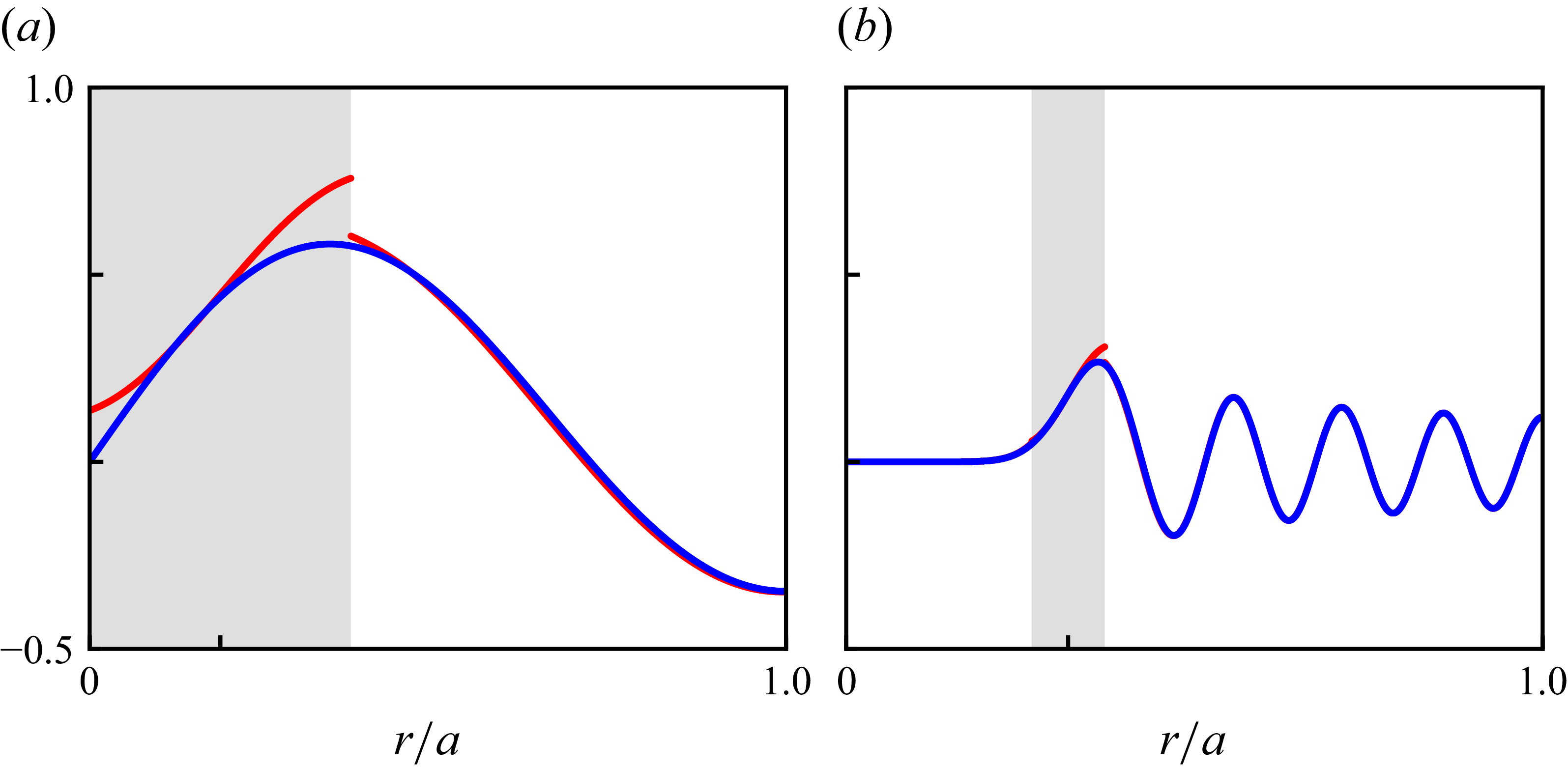
be sufficiently large is to obtain an analytical asymptotic solution to the Bessel integral. Figure 2 presents the asymptotic approximation of Bessel functions and the corresponding exact calculations for varying mode orders. Our numerical calculations show that, for
 $m \geqslant 1$
and
 $n \geqslant 2$
, (2.7c
) is in very good agreement with the exact solution. When
 $n = 1$
but
 $m \neq 0$
, since
 $j'_{m,1} \sim m (1 + 0.8086165 m^{- {2}/{3}})$
(Olver Reference Olver1968) and thus
 $\varrho _{m,n} (1 + m^{- {2}/{3}}) \geqslant j'_{m,1}$
, the outer annulus, at which
 $\varrho _{m,n} (1 + m^{- {2}/{3}}) \lesssim r \leqslant a$
, shrinks to a circular line. The comparison between the exact solution and the numerical calculations using (2.7c
) at
 $r = a$
yields a maximum relative error
 $6 \,\%$
, which decreases as
 $m$
increases.
Comparison of
 $J_{m} (\alpha _{m,n} r)$
between the exact (blue) and asymptotic (red) calculations. The subscale of the horizontal axis denotes
 $\varrho _{m,n}/a$
. The shaded region indicates the range of applicability of (2.7b
). Here (a)
 $(m, n ) = (1, 2 )$
, (b)
 $(m, n ) = (15, 9 )$
.

The above numerical results may be justified by Matviyenko’s (Reference Matviyenko1993) paper, according to which the expansions of
 $J_{m} (z)$
with respect to the large parameter
 $m$
for
 $z \gtrless m$
are not expansions in inverse powers of
 $m$
, but turn out to be uniform expansions in inverse powers of
 $(z - m ) z^{- {1}/{3}}$
for
 $z \gt m$
and
 $(m - z ) m^{- {1}/{3}}$
for
 $z \lt m$
. Therefore, even if
 $m$
is not large, errors beyond the boundary layer (with thickness
 $O (m^{- {2}/{3}})$
, (Ludwig Reference Ludwig1970)) surrounding the caustic surface may still be negligible. Furthermore, Matviyenko (Reference Matviyenko1993) proves that, for any
 $z \gt 0$
and
 $m = 0$
, the asymptotic expansions of Bessel/Hankel functions with respect to
 $m$
and
 $z$
are identical. Hence, the outer annulus of
 $J_{0} (z)$
covers almost the entire region, and the large
 $z$
approximation ensures that the relative error is bounded by
 $\mathrm{e}^{1/4z}/(4z)$
. For modes with
 $m = 0$
and
 $n \neq 0$
, there is always
 $j'_{0,n} \geqslant 3.8317 \cdots$
at the shroud, ensuring that the relative error in this vicinity
 ${\leqslant} 7 \,\%$
, which decreases sharply as
 $n$
increases. Therefore, (2.7c
) provides a remarkable approximation for all non-plane modes near the shroud. For plane waves, the asymptotic approximation is superfluous.
2.3. Energy propagation velocity
We shall now derive the asymptotic expression for the energy propagation velocity of the incident wave in the vicinity of the shroud. The angle of the energy propagation velocity, as outlined in the introduction, is critical for the subsequent GTD analysis of ray tracing in that it determines both the direction of the incident wave and the cone parameter along which the diffracted rays propagate. The reason we concentrate on the energy propagation velocity near the shroud is that the diffracted field is completely determined by the local properties of the incident wave at the rim of the duct opening.
For
 $\varrho _{m,n} (1 + m^{- {2}/{3}}) \lesssim r \leqslant a$
, we can use (2.7) to decompose the modal wave
 $p_{m,n}$
as the sum of two progressing waves,
 ${}^{+} p_{m,n} + {}^{-} p_{m,n}$
, in the radial dimension,
 \begin{align} {}^{\pm } p_{m,n} \left (k, \boldsymbol{x} \right ) & \sim P_{m,n}^{\pm } \frac {1}{\sqrt {2 \pi \alpha _{m,n} r \sqrt {1 - m^{2}/(\alpha _{m,n}^{2} r^{2})} } } \mathrm{e}^{- \mathrm{i} [\omega t - {{\varPsi }}_{m,n}^{\pm } \left (r \right ) - m \theta - \mu _{m,n}^{\pm } z]} \notag \\ & \sim P_{m,n}^{\pm } \frac {H_{m}^{(1,2)} (\alpha _{m,n} r)}{2} \mathrm{e}^{- \mathrm{i} (\omega t - m \theta - \mu _{m,n}^{\pm } z)}, \end{align}
where
 \begin{equation} {{\varPsi }}_{m,n}^{\pm } \left (r \right ) \sim \pm \left (\alpha _{m,n} r \sqrt {1 - \frac {m^{2} }{\alpha _{m,n}^{2} r^{2}} } - m \mathrm{cos}^{-1} \frac {m}{\alpha _{m,n} r} - \frac {\pi }{4} \right )\!, \end{equation}
and
 $H_{m}^{(1)} (\boldsymbol{\cdot })$
and
 $H_{m}^{(2)} (\boldsymbol{\cdot })$
denote the Hankel function of the first and second kinds, respectively, of the integer order
 $m$
. The superscripts ‘
 $+$
’ and ‘
 $-$
’ in (2.8) indicate whether the wave is propagating in the positive or negative direction along the indicated axis. Thanks to the inequality
 $\alpha _{\forall m,\forall n} a \geqslant |m|$
(Olver Reference Olver1968) and the constraint
 $r \gtrsim \varrho _{m,n} (1 + m^{- {2}/{3}})$
, the monotonic phase function,
 ${{\varPsi }}_{m,n} (r )$
, is guaranteed to be real-valued in the outer annulus.
The phase expression specified in (2.8) implies that the wavenumber vector of each progressing component is
 \begin{equation} {}^{\pm } \boldsymbol{k}_{m,n} \sim \boldsymbol{\nabla }[{{\varPsi }}_{m,n}^{\pm } \left (r \right ) + m \theta + \mu _{m,n}^{\pm } z] = \pm \sqrt {\alpha _{m,n}^{2} - \frac {m^{2}}{r^{2}}} \boldsymbol{e}_{r} + \frac {m}{r} \boldsymbol{e}_{\theta } + \mu _{m,n}^{\pm } \boldsymbol{e}_{z}. \end{equation}
It is then found that the dispersion relation (2.4) agrees asymptotically with
 $\omega \sim \boldsymbol{u}_{0} \boldsymbol{\cdot }{}^{\pm } \boldsymbol{k}_{m,n} + c_{0} |{}^{\pm } \boldsymbol{k}_{m,n}|$
. The latter is precisely the dispersion equation of geometrical acoustics (Ostashev & Wilson Reference Ostashev and Wilson2015, (3.21)). Moreover, we can check that the amplitude of the progressing component
 ${}^{\pm } p_{m,n}$
satisfies the transport equation of geometrical acoustics (Ostashev & Wilson Reference Ostashev and Wilson2015, (3.25)):
 $2 {}^{\pm } \boldsymbol{c}_{m,n} \boldsymbol{\cdot }\boldsymbol{\nabla }(\boldsymbol{\cdot }) + (\boldsymbol{\cdot }) \boldsymbol{\nabla }\boldsymbol{\cdot }{}^{\pm } \boldsymbol{c}_{m,n} = 0$
, where
 \begin{equation} {}^{\pm } \boldsymbol{c}_{m,n} := \frac {\partial \omega }{\partial {}^{\pm } \boldsymbol{k}_{m,n} } \sim \boldsymbol{u}_{0} + c_{0} {}^{\pm } \boldsymbol{\kappa }_{m,n} \end{equation}
is the group velocity of
 ${}^{\pm } p_{m,n}$
, and
 ${}^{\pm } \boldsymbol{\kappa }_{m,n} := {}^{\pm } \boldsymbol{k}_{m,n}/|{}^{\pm } \boldsymbol{k}_{m,n}|$
is the unit vector normal to the modal wavefront. The foregoing findings indicate that (2.8) represents a ray field. The energy conservation equation can then be derived from geometrical acoustics’ eikonal and transport equations, with acoustic energy propagating at the group velocity.
In § 2.2 of the study, we have bypassed the plane wave scenario. However, it is evident that (2.10), when taking the plane wave limit (
 $m \to 0$
and
 $\alpha _{m,n} \to 0$
), recovers the wavenumber vector derived directly from the plane wave itself. Thus, the analysis in this subsection applies to all types of modal waves, whether plane or non-plane, spinning or non-spinning.
Upon further simplification of the energy propagation angles
 $\chi _{m,n}^{i} := \cos ^{-1} ({}^{\pm } \boldsymbol{c}_{m,n} \boldsymbol{\cdot }\boldsymbol{e}_{i}/|{}^{\pm } \boldsymbol{c}_{m,n}|)$
and taking note of (2.4), we obtain
 \begin{align} \chi _{m,n}^{r \pm } \left (r \right ) \sim \cos ^{-1} \frac {\pm \sqrt {(1 - {{\varDelta }}_{m,n}^{2}) - \beta _{0}^{2} m^{2}/(k r)^{2}} }{\sqrt {1 - \big(1 - \beta _{0}^{2}\big) {{\varDelta }}_{m,n}^{2} }}, \end{align}
and
 \begin{align} \chi _{m,n}^{\theta } \left (r \right ) \sim \cos ^{-1} \frac {\beta _{0} m/(k r)}{\sqrt {1 - \big(1 - \beta _{0}^{2}\big) {{\varDelta }}_{m,n}^{2} }}, \quad \chi _{m,n}^{z \pm } \left (r \right ) \sim \cos ^{-1} \frac {\pm \beta _{0} {{\varDelta }}_{m,n} }{\sqrt {1 - \big(1 - \beta _{0}^{2}\big) {{\varDelta }}_{m,n}^{2} }}, \end{align}
where the principal value of
 $\cos ^{-1} (\boldsymbol{\cdot })$
is implied, and
 ${{\varDelta }}_{m,n} := \sqrt {1 - [\alpha _{m,n}/(k/\beta _{0})]^{2}}$
. Figure 3 shows the schematic values of these angles at the shroud. These angles lay the groundwork for our upcoming GTD analysis. Note that, although both
 ${}^{+} p_{m,n}$
and
 ${}^{-} p_{m,n}$
individually transport acoustic energy of the same strength in the radial direction, the net effect is zero. This is understandable since
 $J_{m}$
supplies a stationary wave (Chapman Reference Chapman1994).
Side and end views of the angles of the group velocity vector of
 ${}^{\pm } p_{m,n}$
. The effect of the duct rim is to diffract the incident wave, producing a cone of diffracted waves that satisfy the law of diffraction (Keller Reference Keller1957, Reference Keller1958, Reference Keller1962). Approximately one quarter of the rays on the Keller cone point backwards into the duct to produce the reflected field. The remaining rays point outwards from the duct and synthesise the radiated field.

3. Radiation from the opening
In a realistic turbofan engine, the duct will be of finite length, and the radiation and reflection from the duct termination is what matters most, which we shall deal with in this section and the next one.
We consider the Prandtl–Glauert transformation, a coordinate stretching technique, i.e.
 \begin{equation} \bar {x} = x, \quad \bar {y} = y, \quad \bar {z} = \frac {z}{\beta _{0}}, \quad \bar {k} = \frac {k}{\beta _{0}}, \quad \check {\phi } (\bar {k}, \bar {\boldsymbol{x}}) \mathrm{e}^{- \mathrm{i} \bar {k} M_{0} \bar {z}} = \hat {\phi } (k, \boldsymbol{x}), \end{equation}
to transform the temporal Fourier transform of (2.1),
 $[{\nabla} ^{2} + (k + \mathrm{i} M_{0} \boldsymbol{e}_{z} \boldsymbol{\cdot }\boldsymbol{\nabla })^{2}] \hat {\phi } = 0$
, into the Helmholtz equation,
 \begin{equation} \big(\bar {{\nabla} }^{2} + \bar {k}^{2}\big) \check {\phi } = 0. \end{equation}
The asymptotic solution to (3.2) is provided in Appendix A. The solution to the original convection problem is finally obtained by the inverse Prandtl–Glauert transformation. Further, because
 $\bar {R} \cos {\bar {\varphi }} = R \cos {\varphi }/\beta _{0}$
and
 $R \sin {\varphi } = \bar {R} \sin {\bar {\varphi }}$
, we get
 \begin{equation} \bar {R} = \frac {R}{\beta _{0}} \sqrt {1 - \big(1 - \beta _{0}^{2}\big) \sin ^{2}{\varphi }}, \quad \bar {\varphi } = \tan ^{-1} \left (\beta _{0} \tan {\varphi } \right ), \quad \bar {\theta } = \theta . \end{equation}
By this convention, geometric quantities in the transformed coordinate system are indicated by an overbar.
The full solution of the diffraction problem, according to the GTD, is
 $\check {p} = \check {p}_{I} + \check {p}_{R} + \check {p}_{D}$
. In addition to the incident and reflected waves of the geometrical acoustic solution
 $\check {p}_{I} + \check {p}_{R}$
, there is an additional diffracted wave
 $\check {p}_{D}$
. We shall later show that the effective incident wave reads
 $\check {p}_{I} \propto H_{m}^{(1)} (\alpha _{m,n} r)$
. On this basis and on account of the law of reflection, we determine that
 $\check {p}_{R} \propto H_{m}^{(2)} (\alpha _{m,n} r)$
. It is obvious that
 $\check {p}_{I}$
and
 $\check {p}_{R}$
are not solutions exterior to the duct that satisfy Sommerfeld’s radiation condition
 \begin{equation} \lim _{\bar {R} \to + \infty } \bar {R} \left (\frac {\partial }{\partial \bar {R}} - \mathrm{i} \bar {k} \right ) \check {p} = 0 \quad \mathrm{uniformly\:in\:all\:directions}. \end{equation}
Therefore, the only contribution to the external acoustic field
 $\check {p}$
is the diffracted wave
 $\check {p}_{D}$
.
Keller (Reference Keller1957, Reference Keller1962) remarks that the edge forms a caustic because diffracted rays of the same cone intersect there, and each point of the edge is a centre of curvature of the diffracted wavefronts; thus one of the principal radii of curvature of the initial wavefront,
 $\bar {\rho }_{2}$
, equals
 $0$
. Hence, from (A1) and (A12), we have
 \begin{equation} \check {p}_{D} (\bar {\sigma }) \sim \big[\bar {\sigma } \big(1 + \bar {\rho }_{1}^{- 1} \bar {\sigma }\big)\big]^{-\frac {1}{2}} \lim _{\bar {\rho }_{2} \to 0} [\sqrt {\bar {\rho }_{2}} \check {p}_{D} \left (0 \right ) \mathrm{e}^{\mathrm{i} \bar {k} s \left (0 \right )}] \mathrm{e}^{\mathrm{i} \bar {k} \bar {\sigma }}, \end{equation}
where
 $\bar {\sigma }$
denotes the distance from the edge,
 $\bar {\rho }_{1}$
the edge caustic distance and
 $s (0 )$
the initial phase of the diffracted ray at the edge. By analogy with the calculation of the reflected and transmitted rays, the GTD postulates the existence of the limit,
 $\lim _{\bar {\rho }_{2} \to 0} [\sqrt {\bar {\rho }_{2}} \check {p}_{D} (0 ) \mathrm{e}^{\mathrm{i} \bar {k} s (0 )}]$
, which is assumed to be proportional to the incident field
 $\check {p}_{I}$
at the point of diffraction. Such a proportionality factor is referred to as the diffraction coefficient
 $\bar {D}$
, which is analogous to the reflection and transmission coefficients, and is obtained by comparison with the asymptotic expansion to the exact solution of a canonical problem, Sommerfeld’s half-plane diffraction problem. This allows us to arrive at
 \begin{equation} \check {p}_{D} (\bar {\sigma }) \sim \sum \frac {1}{\sqrt {\bar {\sigma } \big(1 + \bar {\rho }_{1}^{- 1} \bar {\sigma }\big)} } \bar {D} \check {p}_{I} \mathrm{e}^{\mathrm{i} \bar {k} \bar {\sigma }}, \end{equation}
where the summation is performed over all possible edge-diffracted rays, and the half-plane diffraction coefficient,
 \begin{equation} \bar {D} (\bar {\varphi }_{I}, \bar {\varphi }_{D}; \bar {\beta }_{K}) = - \frac {\mathrm{e}^{\mathrm{i} \pi /4}}{2 \sqrt {2 \pi \bar {k}} \sin {\bar {\beta }_{K}} } \left (\sec {\frac {\bar {\varphi }_{D} + \bar {\varphi }_{I}}{2}} + \sec {\frac {\bar {\varphi }_{D} - \bar {\varphi }_{I}}{2}} \right )\!, \end{equation}
which applies to the Neumann boundary condition in relation to the total field
 $\check {p}$
, is singular at
 $\bar {\varphi }_{D} \pm \bar {\varphi }_{I} = \pi$
. Here,
 $\bar {\varphi }_{I}$
(
 $\bar {\varphi }_{D}$
) is the angle between the edge and the incident (diffracted) ray, and
 $\bar {\beta }_{K}$
denotes the semiangle of the Keller cone, which is defined as the angle between the incident ray and the positive tangent (
 $\boldsymbol{e}_{\theta }$
) to the edge curve.
Taking into account the studies in § 2.3, for modal waves, it is only the radial, outward-progressing component
 $\propto H_{m}^{(1)} (\alpha _{m,n} r)$
that hits the rim of the duct at an incident (polar) angle
 \begin{equation} \bar {\varphi }_{I} \sim \lim _{M_{0} \downarrow 0} \chi _{m,n}^{z +} \left (a \right ) \equiv \sin ^{-1} \frac {\alpha _{m,n}}{\bar {k}} =: \bar {\varphi }_{m,n}. \end{equation}
Regarding the angle
 $\bar {\beta }_{K}$
between the incident ray and the (positive) tangent to the edge (Keller Reference Keller1957, Reference Keller1962), it is merely the no-flow limit of the azimuthal projection angle of the group velocity exiting the duct opening:
 \begin{equation} \bar {\beta }_{K} \sim \lim _{M_{0} \downarrow 0} \chi _{m,n}^{\theta } \left (a \right ) \equiv \cos ^{-1} \frac {m}{\bar {k} a}. \end{equation}
One may check that performing the inverse Prandtl–Glauert transformation to these two angles produces the results given by (2.12).
There are three parameters to be determined,
 $\bar {\sigma }$
,
 $\bar {\varphi }_{D}$
and
 $\bar {\rho }_{1}$
, which shall be found through geometrical considerations. To this end, we need to parametrise the Keller cone to identify the diffracted rays travelling through the observation point
 $\bar {\boldsymbol{x}}$
and get
 \begin{equation} (\bar {R} \sin {\bar {\varphi }} \cos {\bar {\theta }}, \bar {R} \sin {\bar {\varphi }} \sin {\bar {\theta }}, \bar {R} \cos {\bar {\varphi }}) =: \bar {\boldsymbol{x}} \equiv \bar {\boldsymbol{x}}_{V} + \bar {\sigma } \cos {\bar {\beta }_{K}} \bar {\boldsymbol{T}} + \bar {\sigma } \sin {\bar {\beta }_{K}} \bar {\boldsymbol{N}}, \end{equation}
where
 $\bar {\boldsymbol{x}}_{V} = a (\cos {\bar {\theta }_{V}}, \sin {\bar {\theta }_{V}}, 0)$
denotes position of the diffraction point (vertex of the Keller cone),
 $\bar {\sigma } := \left |\bar {\boldsymbol{x}} - \bar {\boldsymbol{x}}_{V} \right |$
is the eikonal of the diffracted rays,
 $\bar {\boldsymbol{T}} = (- \sin {\bar {\theta }_{V}}, \cos {\bar {\theta }_{V}}, 0)$
is the unit vector along the cone axis (i.e. the unit tangent to the edge, for an illustration, see figure 4),
 $\bar {\boldsymbol{N}} = (\cos {\bar {\theta }_{V}} \sin {\bar {\alpha }_{K}}, \sin {\bar {\theta }_{V}} \sin {\bar {\alpha }_{K}}, \cos {\bar {\alpha }_{K}})$
is a unit vector perpendicular to
 $\bar {\boldsymbol{T}}$
and
 $\bar {\alpha }_{K} \in [0, 2 \pi )$
is the angle of rotation around the cone axis. Thus,
 \begin{align} \bar {\sigma } \equiv \bar {R} \sqrt {1 - 2 \frac {a}{\bar {R}} \sin {\bar {\varphi }} \cos {\big(\bar {\theta } - \bar {\theta }_{V}\big)} + \frac {a^{2}}{\bar {R}^{2}} } = \bar {R} - a \sin {\bar {\varphi }} \cos {\big(\bar {\theta } - \bar {\theta }_{V}\big)} + O \big(\bar {R}^{- 1}\big), \end{align}
and
 \begin{equation} \bar {R} \equiv \bar {\sigma } \sqrt {1 + 2 \frac {a}{\bar {\sigma }} \sin {\bar {\alpha }_{K}} \sin {\bar {\beta }_{K}} + \frac {a^{2}}{\bar {\sigma }^{2}} } = \bar {\sigma } + a \sin {\bar {\alpha }_{K}} \sin {\bar {\beta }_{K}} + O \big(\bar {\sigma }^{- 1}\big). \end{equation}
In order to obtain an analytical solution in closed form, our focus is on the distant diffracted field, which allows us to derive an explicit representation of the solution. In this case, the GTD solution
 $\check {p}_{D}$
is equal to to the fundamental solution of (3.2) due to a point source,
 $- \mathrm{e}^{\mathrm{i} \bar {k} \bar {\sigma }}/(4 \pi \bar {\sigma })$
, multiplied by a diffraction pattern function. This illustrates that the characteristics of the acoustic field at a distance are determined by the superposition of (multiple) diffraction point sources. Upon noticing that
 $\bar {R} \cos {\bar {\varphi }} = \bar {\sigma } \sin {\bar {\beta }_{K}} \cos {\bar {\alpha }_{K}}$
and that there is always
 $\bar {\theta }_{V} \leqslant \bar {\theta }$
on the cone, the geometric relation (3.11) is solved to give
 \begin{align} \bar {\sigma }^{1,2} \sim \bar {R} \mp a \sqrt {\sin ^{2}{\bar {\beta }_{K}} - \cos ^{2}{\bar {\varphi }}}, \quad \bar {\theta }_{V}^{1,2} \sim \bar {\theta } - \cos ^{-1} \left (\pm \frac {1}{\sin {\bar {\varphi }} } \sqrt {\sin ^{2}{\bar {\beta }_{K}} - \cos ^{2}{\bar {\varphi }}} \right )\!. \end{align}
These are the asymptotic expressions for the parameters of the propagation trajectory cone of diffracted rays in the far field.
The possible positions of the diffraction point within the far-field approximation. When the observer is outside the duct and behind the duct opening, only a portion of it is visible. The part of the duct edge that is occluded (not visible) from the observer’s perspective is shown in a dashed line. The tangential direction at the diffraction point on the duct rim is aligned with the cone axis vector
 $\bar {\boldsymbol{T}}$
(blue vectors). Diffracted rays that propagate along the Keller cone but do not point towards the observer
 $\bar {\boldsymbol{x}}$
do not contribute to the acoustic field there. There are two sets of possible solutions for each ray (red lines), which is consistent with (3.11) and (3.12). However, only one set is physically realistic.

Since edge-diffracted rays propagate according to Fermat’s principle for edge diffraction (Keller Reference Keller1957, Reference Keller1958, Reference Keller1962), the diffracted rays governing the acoustic field in a homogeneous medium follow the shortest path. When we draw two spheres centred on the observer
 $\bar {\boldsymbol{x}}$
, with radii
 $\bar {\sigma }^{1} \lt \bar {R}$
and
 $\bar {\sigma }^{2} \gt \bar {R}$
and within the Keller cone, their intersections with the duct rim (schematically plotted in figure 4) correspond to two sets of solutions. The acoustic field thus consists of contributions from two diffracted rays. However, when the observer is behind the duct opening where
 $\pi /2 \lt \bar {\varphi } \lt 3 \pi /2$
, only one set of these solutions with the shorter eikonal
 $\bar {\sigma }^{1}$
is physically possible due to the shielding effect of the duct. We also observe from figure 4, by its definition, that
 $\bar {\varphi }_{D}^{1,2} \sim \pi \pm \bar {\varphi }$
.
The non-zero principal radius of curvature of the wavefront for the diffracted rays is determined by comparing (3.10) and (A8), and then evaluating (A11) to obtain, in the distant field,
 \begin{equation} \bar {\rho }_{1}^{1,2} \equiv - \frac {|b_{\!J}|}{a_{\!J}} = \frac {a \sin {\bar {\beta }_{K}}}{\sin {\bar {\alpha }_{K}^{1,2}} } \sim \pm \frac {a \sin ^{2}{\bar {\beta }_{K}}}{\sqrt {\sin ^{2}{\bar {\beta }_{K}} - \cos ^{2}{\bar {\varphi }}} }, \end{equation}
where the asymptotic expression for
 $\bar {\alpha }_{K}$
is derived from (3.11b
) and (3.12). The positive (negative) radius of curvature of ray
 $1$
(
 $2$
) indicates that it is diverging (converging).
Substituting all of the energy and geometric parameters, as well as the incident wave solution given by (2.8) and taken at the duct rim where
 $\bar {\boldsymbol{x}} = (a, \bar {\theta }_{V}^{1,2}, 0)$
, into (3.6), we have
 \begin{equation} \check {p}_{D} (\bar {k}, \bar {\boldsymbol{x}}) \sim \frac {a}{\bar {R}} P_{m,n} \mathcal{D}_{m,n} (\bar {k} a, \bar {\varphi }) \mathrm{e}^{\mathrm{i} (\bar {k} \bar {R} + m \bar {\theta })}, \quad \bar {R}/a \gg 1, \end{equation}
where
 \begin{align} \mathcal{D}_{m,n} (\bar {k} a, \bar {\varphi }) & = \frac {J_{m} (\bar {k} \sin {\bar {\varphi }_{m,n}} a) \mathrm{e}^{- \mathrm{i} m \pi /2} }{4 \sqrt {2 \pi \bar {k} a \sqrt {\sin ^{2}{\bar {\beta }_{K}} - \cos ^{2}{\bar {\varphi }}} } } \left [\mathrm{e}^{- \mathrm{i} \tau _{m} (\bar {k} a, \bar {\varphi })} - \mathrm{e}^{\mathrm{i} \tau _{m} (\bar {k} a, \bar {\varphi })} H \left (\frac {\pi }{2} - \bar {\varphi } \right ) \right ] \notag \\ & \qquad \qquad \qquad \qquad \qquad \times \left (\csc {\frac {\bar {\varphi } - \bar {\varphi }_{m,n}}{2}} + \csc {\frac {\bar {\varphi } + \bar {\varphi }_{m,n}}{2}} \right )\!, \end{align}
and
 \begin{align} \tau _{m} (\bar {k} a, \bar {\varphi }) = \bar {k} a \sqrt {\sin ^{2}{\bar {\beta }_{K}} - \cos ^{2}{\bar {\varphi }}} + m \cos ^{-1} \left (\frac {1}{\sin {\bar {\varphi }} } \sqrt {\sin ^{2}{\bar {\beta }_{K}} - \cos ^{2}{\bar {\varphi }}} \right ) - m \frac {\pi }{2} - \frac {\pi }{4}. \end{align}
Here,
 $H (\boldsymbol{\cdot })$
denotes the Heaviside unit function concerning the shielding of ray
 $2$
, and the asymptotic approximation
 $Y_{m} (\alpha _{m,n} a) \sim - J'_{m} (\alpha _{m,n} a) = 0$
, being used for the incident ray, is implied by (2.7c
) and (2.8). Here,
 $Y_{m} (\boldsymbol{\cdot })$
is the
 $m$
th-order Bessel function of the second kind.
The current asymptotic solution (3.14b
) has two issues that need to be addressed. Firstly, the extreme surface of the Keller cone, for which
 $\bar {\varphi } = \pi /2 \pm \bar {\beta }_{K}$
, denotes the location of the caustic surface. The diffracted field is infinite there because the geometrical divergence of the diffracted rays,
 $\sqrt {\bar {\sigma } (1 + \bar {\rho }_{1}^{- 1} \bar {\sigma })} \sim \bar {\sigma } \bar {\rho }_{1}^{- {1}/{2}}$
, is zero. Secondly, it can be seen that
 $\bar {\varphi } = \bar {\varphi }_{m,n}$
is both a zero and a maximum of
 $\sin {\tau _{m} (\bar {k} a, \bar {\varphi })}$
, from which there follows
 $\mathcal{D}_{m,n} (\bar {k} a, \bar {\varphi }_{m,n} + 0^{\pm }) \propto \sin {[\tau _{m} (\bar {k} a, \bar {\varphi }_{m,n} + 0^{\pm })]} \times \csc {0^{\pm }}$
, i.e.
 $\mathcal{D}_{m,n} (\bar {k} a, \bar {\varphi })$
diverges at
 $\bar {\varphi } = \bar {\varphi }_{m,n}$
. This is the shadow boundary of ray
 $1$
and the reflection boundary of ray
 $2$
. Here,
 $0^{+}$
and
 $0^{-}$
refer, respectively, to the upper and lower limits.
In his treatment of caustics and shadow boundaries, Keller (Reference Keller1962) replaced the Hankel approximation of a cylindrical function with its exact counterpart obtained from a canonical problem in pursuit of a finite value. We shall resolve the above issues in the same spirit. The GTD solution (3.14b ) implies Hankel’s asymptotic approximations for cylindrical functions. In view of the asymptotic expression
 \begin{equation} {H_{m}^{(1,2)}}' \left (m z \right ) \sim \pm \mathrm{i} \sqrt {\frac {2 \sqrt {1 - z^{- 2}}}{\pi m z}} \mathrm{e}^{\left [\pm \mathrm{i} \left (m z \sqrt {1 - z^{- 2} } + m \cos ^{-1} \sqrt {1 - z^{- 2}} - m \pi /2 - \pi /4 \right ) \right ]} \end{equation}
obtained from (2.7c
) for
 $z \gtrsim 1 + m^{- {2}/{3}}$
, these are identified as
 $({1}/{2}) {H_{m}^{(2)}}' (\bar {k} a \sin {\bar {\varphi }})$
and
 $({1}/{2}) {H_{m}^{(1)}}' (\bar {k} a \sin {\bar {\varphi }})$
, for diffracted rays
 $1$
and
 $2$
, respectively. It then follows from the Taylor expansion and Bessel’s equation
 $z^{2} J''_{m} (z ) + z J'_{m} (z ) + (z^{2} - m^{2}) J_{m} (z ) = 0$
that the aforementioned issues can be overcome if we replace the asymptotic approximations of the Hankel functions with their exact counterparts. The consequence is
 \begin{align} \mathcal{D}_{m,n} & (\bar {k} a, \bar {\varphi }) \sim \frac {\mathrm{i}^{1 - m} J_{m} (\alpha _{m,n} a)}{4} \left (\csc {\frac {\bar {\varphi } - \bar {\varphi }_{m,n}}{2}} + \csc {\frac {\bar {\varphi } + \bar {\varphi }_{m,n}}{2}} \right ) \notag \\ & \qquad \times \left [J'_{m} (\bar {k} a \sin {\bar {\varphi }}) H \left (\frac {\pi }{2} - \bar {\varphi } \right ) + \frac {1}{\pi \bar {k} a \sin {\bar {\varphi }} {H_{m}^{(1)}}' (\bar {k} a \sin {\bar {\varphi }}) } H \!\left (\bar {\varphi } - \frac {\pi }{2} \right ) \right ]\!. \end{align}
In order that the diffracted field is finite near
 $\bar {\varphi } = \pi$
, we have replaced
 $({1}/{2}) {H_{m}^{(2)}}' (\bar {k} a \sin {\bar {\varphi }})$
with its Hankel approximation, given that
 $({1}/{2}) {H_{m}^{(2)}}' (z) \sim 1/[\pi z {H_{m}^{(1)}}' (z)]$
. We have compared the results of (3.14b) and (3.17) numerically. The latter has been found to significantly improve predictions in the earlier mentioned key regions, while predictions elsewhere have remained almost identical to those of the former.
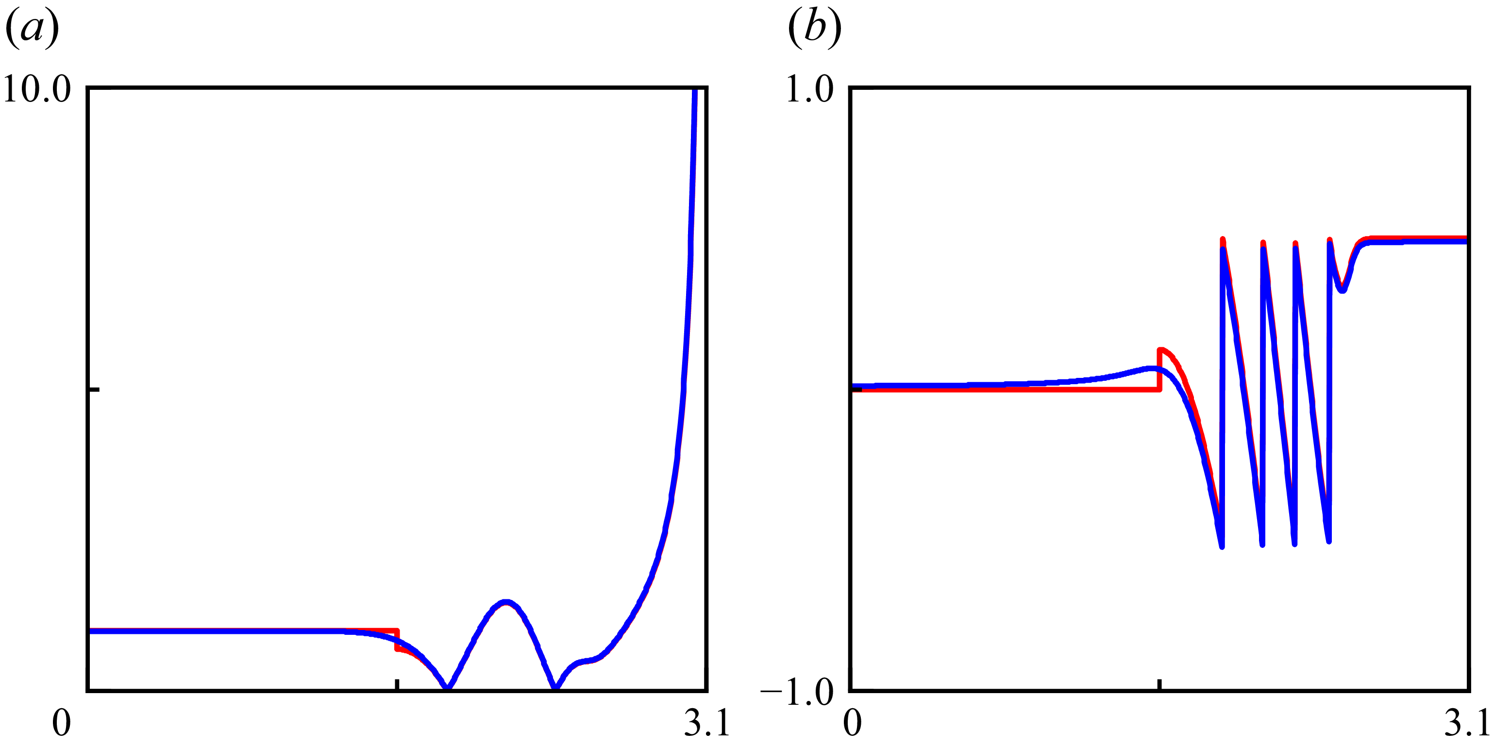
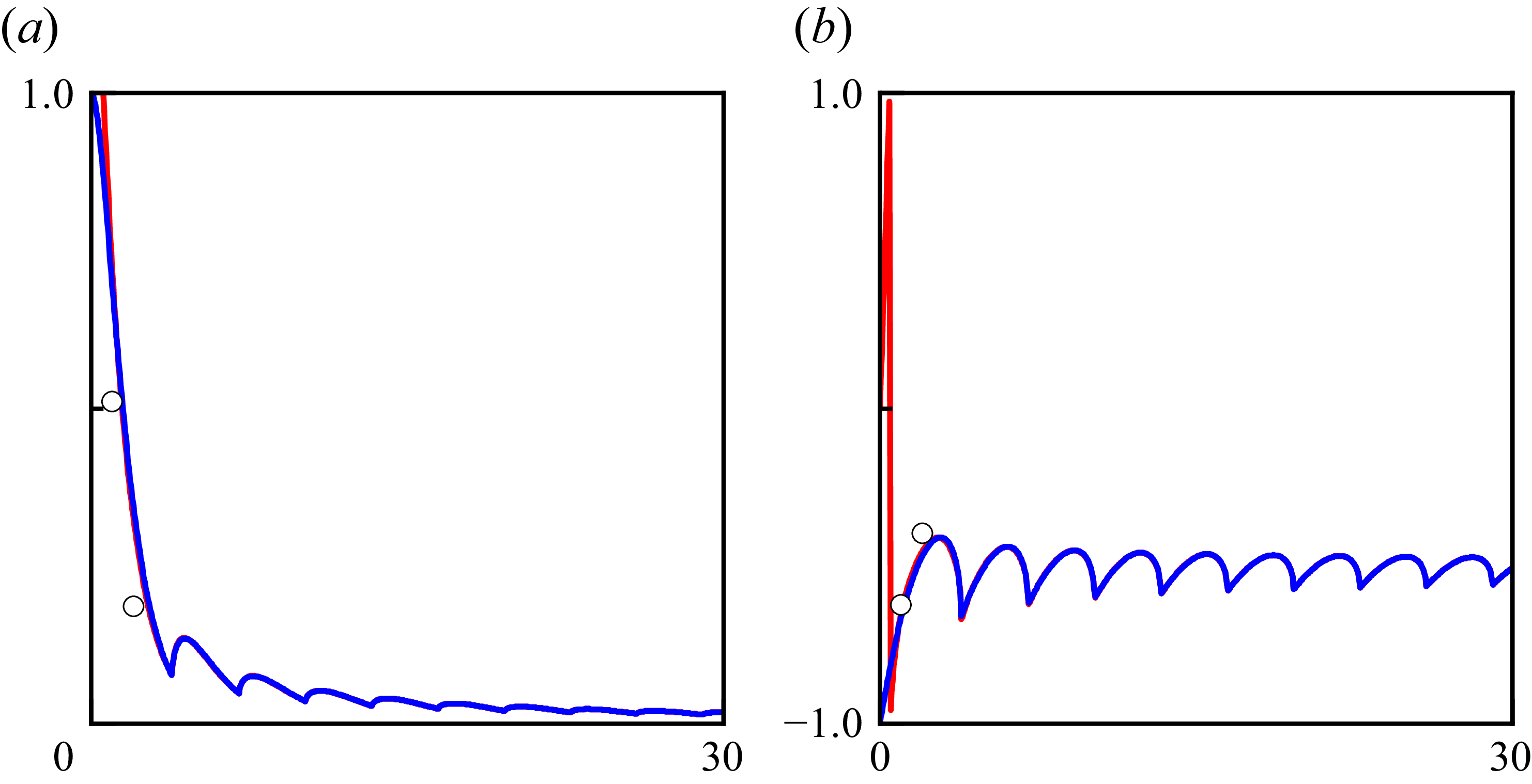
Comparison of the asymptotic (red line) and exact (blue line) calculations of the plus function
 $K_{+}^{(m)} (\bar {k} \cos {\bar {\varphi }})$
for the case
 $\bar {k} a = 17$
and
 $m = 10$
. Here (a)
 $|K_{+}^{(m)} (\bar {k} \cos {\bar {\varphi }})|$
, (b)
 $\pi ^{- 1} \arg K_{+}^{(m)} (\bar {k} \cos {\bar {\varphi }})$
.

In Appendix B, the Wiener–Hopf solution (B23) for the same radiation problem is derived. The exact solution (B23) involves split functions
 $K_{\pm }^{(m)} (\kappa )$
defined by (B9), making it difficult to disclose the structure of the acoustic field. (We subscript the Wiener–Hopf kernel and its factorisations with ‘
 $m$
’ to indicate their dependence on the azimuthal-mode order
 $m$
.) To this end, one possible approach is to utilise the universal function of Weinstein (Reference Weinstein1969), which is derived by first changing the variable of integration, then deforming the contour into a path of steepest descent, and finally using Hankel’s approximations for the cylindrical functions. This leads to, for
 $\cos {\bar {\varphi }} \gt 0$
and
 $\bar {k} a \gtrsim |m|$
,
 \begin{align} \ln {K_{+}^{(m)} (\bar {k} \cos {\bar {\varphi }})} \sim \frac {1}{2 \pi \mathrm{i} } \int _{- \infty }^{+ \infty } \ln {\Big \{1 - \mathrm{e}^{2 \mathrm{i} [\arg {H_{m}^{(1)}}' (\bar {k} a) - \pi /2] - \xi ^{2}/2} \Big \}} \frac{\mathrm{d} \xi }{\xi - \sqrt {2 \bar {k} a} \mathrm{e}^{\mathrm{i} \pi /4} \cos {\bar {\varphi }}}. \end{align}
Further simplification was achieved by Bowman (Reference Bowman1970) who expanded the logarithm as a Mercator series and integrated the result term by term, giving
 \begin{align} K_{+}^{(m)} (\bar {k} \cos {\bar {\varphi }}) \sim 1 & + O \big((\bar {k} a)^{- \frac {1}{2}}\big) O (1/\cos {\bar {\varphi }}) \notag \\ & \Leftrightarrow K_{-}^{(m)} (\bar {k} \cos {\bar {\varphi }}) \sim K^{(m)} (\bar {k} \cos {\bar {\varphi }}) + O \big((\bar {k} a)^{- \frac {1}{2}}\big) O (1/\cos {\bar {\varphi }}). \end{align}
(Though the author explicitly discussed only the case of
 $m = 0$
.) This expansion suggests that, at high frequencies, the Wiener–Hopf kernel
 $K^{(m)} (\kappa )$
introduced by (B8) behaves asymptotically like a minus/plus function for
 $\kappa \gtrless 0$
, given its even-function property:
 $K_{+}^{(m)} (- \kappa ) = K_{-}^{(m)} (\kappa )$
(Noble Reference Noble1958, p. 17). Clearly, (3.19) breaks down near
 $\bar {\varphi } = \pi /2$
due to the shielding of ray
 $2$
, a matter we shall address shortly. This breakdown is actually not attributable to Bowman’s expansion. Rather, it is attributable to the saddle point approximation, as evidenced by the use of the Plemelj formula. The leading term of the Wiener–Hopf solution (B23) employing the Weinstein–Bowman approximation (3.19) for the split functions is therefore found to be in agreement with the GTD solution (3.17) for primary diffraction.
To verify the accuracy of the Weinstein–Bowman approximation (3.19), figure 5 pictures the results of (3.19) and the exact calculation of the plus function. Note that in the calculation of the integral (B9), the Wiener–Hopf kernel has several zeros along the integration contour, as well as a branch cut along the interval
 $(- \infty , - \bar {k}] \cup [+ \bar {k}, + \infty )$
. To facilitate numerical calculations, we employ the method of deformed integration contour proposed by Rienstra (Reference Rienstra1984), adopted by Gabard & Astley (Reference Gabard and Astley2006) for their Wiener–Hopf analysis, and recently improved by Rienstra (Reference Rienstra2022). See Appendix C for details.
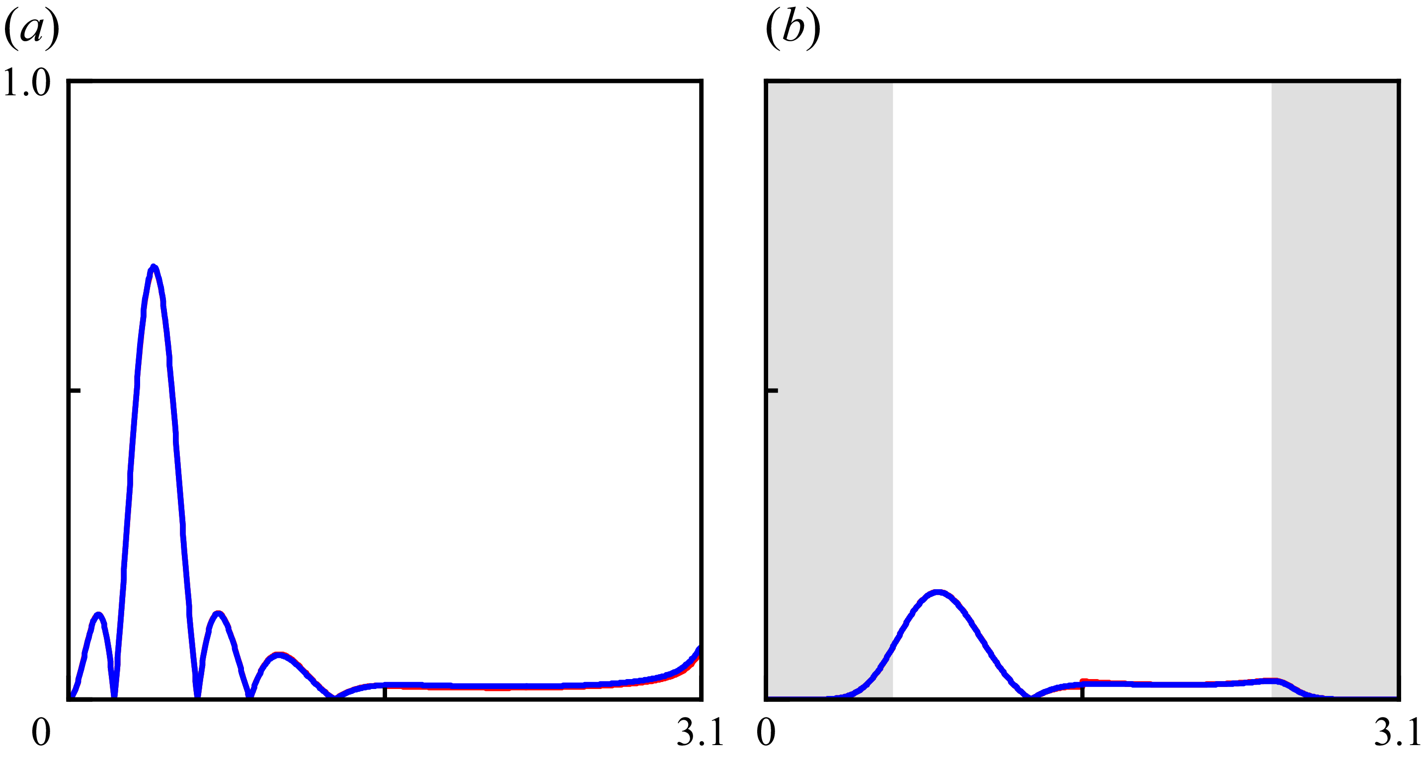
Figure 6 depicts a comparison of the GTD solution (3.17) and the Wiener–Hopf solution (B23) at high frequencies. The two analytical solutions are in satisfactory agreement, except near the sideline, where the illumination-shadow boundary of ray
 $2$
is. This results in a jump discontinuity and a nearby deviation in the predictions. The shielding of ray
 $2$
by the duct is not abrupt, but rather a continuous process that takes place through a boundary layer, as evidenced by the Wiener–Hopf solution. Furthermore, we highlight that the asymptotic analysis based upon § 2 still produces satisfactory results even when the outer annulus for progressing waves shrinks to a circular line, for which the radial order
 $n = 1$
.
Comparison of directivity profiles
 $|\mathcal{D}_{m,n} (\bar {k} a, \bar {\varphi })|$
, where the red and blue solid lines are calculated according to the GTD solution (3.17) and the Weiner–Hopf solution (B23), respectively. The shaded regions are from
 $0$
to
 $\pi /2 - \bar {\beta }_{K}$
and from
 $\pi /2 + \bar {\beta }_{K}$
to
 $\pi$
. Here (a)
 $(m, n ) = (0, 3 )$
,
 $\bar {k} a = 17$
; (b)
 $(m, n ) = (10, 1 )$
,
 $\bar {k} a = 17$
.

A comparison of analytical and experimental results is now presented for an unflanged duct. The duct test apparatus incorporating a spinning mode synthesiser is mounted in the flow duct facility at the Aircraft Noise Reduction Laboratory of NASA Langley Research Center and extends into the anechoic chamber. The acoustic measurements include the far-field directivity and the reflection coefficient. The details are referenced to Ville & Silcox (Reference Ville and Silcox1980). The far-field directivity data have not been normalised with respect to the amplitudes of the incident modes, which were not reported for this experiment. The predicted sound pressure level curve is therefore normalised with respect to the largest value of the measured sound pressure level curve. Presented in figure 7 is a comparison of the modal radiated field, with remarkable agreement observed between the analytical and experimental data. The spinning radiated field not exhibiting the expected exponential decay around the centreline is believed to be due to plane wave leakage (Ville & Silcox Reference Ville and Silcox1980).
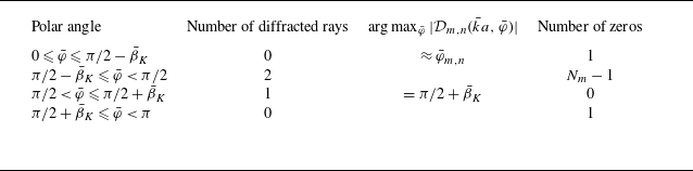
In closing this section, we shall summarise the typical structure of the radiated field in table 1. The presence of fore-arc zeros at
 $\bar {\varphi }_{m,s \neq n}$
and the interlacing lobes from there appears to be a consequence of the strong interference of the two diffracted rays, which also gives rise to a peak intensity near
 $\bar {\varphi }_{m,n}$
. In the aft arc, there is no ray
 $2$
and therefore a broad lobe. The aft-arc directivity reaches its maximum intensity at the end of the broad lobe. In the special case of
 $m = 0$
, the solution is non-zero at
 $\bar {\varphi } = \pi$
for all
 $n$
, and is only non-zero at
 $\bar {\varphi } = 0$
for
 $n = 1$
.
Typical structure of the radiated field for a given mode in an unflanged duct. The integer
 $N_{m} := \max {\{n \in \mathbb{N}^{+}|\alpha _{m,n} \lt \bar {k} \}}$
refers to the highest radial order of a given azimuthal-order mode cut on by the duct.

Comparison of the predicted and measured sound pressure levels. Key as figure 6. Data from the experimental study is indicated by the black circles. The shaded regions are from
 $0$
to
 $\pi /2 - \bar {\beta }_{K}$
. Here (a)
 $(m, n ) = (0, 1 )$
,
 $\bar {k} a = 3.76$
; (b)
 $(m, n ) = (1, 1 )$
,
 $\bar {k} a = 5.29$
; (c)
 $(m, n ) = (6, 1 )$
,
 $\bar {k} a = 11.14$
.

4. Reflection from the opening
Because a portion of the Keller cone is located within the duct (figure 3), the incident modal wave will be partially reflected back into it. The reflected wave is in the form of cylindrical waves.
Following the law of reflection, we may determine that there is no reflected wave of the incident wave existing within the duct. Thus, we only need to consider the reflected wave due to diffraction, starting with the primary diffraction. Recall that, when the diffracted wave is cylindrical,
 $\bar {\rho }_{1} = \infty$
((Keller Reference Keller1958) since the exact solution to the two-dimensional Helmholtz equation decays as a cylindrical wave in the far field), and (3.6) becomes
 \begin{equation} \check {p}_{D} \sim \sum - \frac {1}{\sin {\bar {\beta }_{K}}} \left (\sec {\frac {\bar {\varphi }_{D} + \bar {\varphi }_{m,n}}{2}} + \sec {\frac {\bar {\varphi }_{D} - \bar {\varphi }_{m,n}}{2}} \right ) \check {p}_{I} \frac {\mathrm{e}^{\mathrm{i} (\bar {k} \bar {\sigma } + \pi /4}) }{2 \sqrt {2 \pi \bar {k} \bar {\sigma }} }. \end{equation}
When the observer is far away from the opening, it becomes cumbersome to keep track of, in addition to direct diffraction, and add up the multiple reflections. To simplify the problem, let us consider the simplest case:
 $m \ll \bar {k} a \Leftrightarrow \bar {\beta }_{K} \sim \pi /2$
. In this instance, the Keller cone will asymptotically overlap the meridional plane, enabling us to consider the diffracted waves as propagating in two dimensions. We see that the total diffracted field is constituted by the fundamental solution of (3.2) for two dimensions due to a line source of unit strength,
 $-\mathrm{i} H_{0}^{(1)} (\bar{k} \bar{\sigma})/4 \sim - \mathrm{e}^{\mathrm{i} (\bar{k} \bar{\sigma} + \pi/4)}/(2 \sqrt{2 \pi \bar{k} \bar{\sigma}})$
for large
 $\bar {k} \bar {\sigma }$
, in conjunction with a diffraction pattern function. According to (3.12) and recalling that ray
 $2$
is visible to an observer inside the duct, the duct rim and the meridional plane intersect at two points that constitute diffraction sources:
 $\bar {\theta }_{V}^{1,2} \sim \bar {\theta } - \cos ^{-1} (\pm 1 )$
. Their phases therefore differ by
 $\mathrm{e}^{- \mathrm{i} m \pi }$
. Accordingly,
 $\bar{\varphi}_{D}^{1,2} \sim \bar{\varphi}$
.
Image sources and the reflected ray path (plot up to double reflection only) in the meridional plane
 $(\bar {r}, \bar {z})$
. The intensity of diffracted rays varies with the angle at which they are emitted from the diffraction sources. We are accustomed to referring to diffraction sources distant from (close to) the observer as upper (lower) sources.

Tracing all the direct and multiply reflected rays and adding their fields together is equivalent to summing the fields from an infinite set of images of the line source. This is shown in figure 8. To account for the focusing of cylindrical rays due to the curvature of the duct rim, a caustics factor shall be incorporated into the diffraction solution. Our work on in-duct acoustic fields has shown that this factor is independent of the axial direction, since the ray amplitude only varies radially by a factor of
 $1/\sqrt {\bar {r}}$
in the outer annulus. We assume that this variation applies throughout the radial position, which would be possible if the radial order
 $n$
were much larger than the azimuthal order
 $m$
. This actually corresponds to the case where the caustic radius
 $m/\alpha _{m,n}$
of modal waves (cf. Chapman Reference Chapman1994) asymptotically approaches zero, resulting in the formation of a caustic line along the duct axis. Although the constraint of a large radial order limits the generality of the diffraction solutions, the final solution may be refined by replacing the sinusoidal components with their exact Bessel counterparts. Now, considering that the reality sources are situated at
 $\bar {r} = a$
, the amplitude of the diffracted rays within the duct should then be multiplied by an additional factor of
 $\sqrt {a/\bar {r}}$
. Therefore, the diffracted field arising from primary diffraction writes as
 \begin{align} \check{p}_{D} & \sim - \frac{\mathrm{i}}{4} \sqrt{\frac{a}{\bar{r}}} \sum_{j = 0}^{+ \infty} \mathrm{e}^{- \mathrm{i} (m + 1/2) j \pi} 2 \Big[\mathrm{e}^{- \mathrm{i} (m + 1/2) \pi} \mathscr{P}_{m,n} (\bar{\varphi}_{j}^{+}) H_{0}^{(1)} (\bar{k} \bar{\sigma}_{j}^{+}) \notag \\ & \qquad \qquad \qquad \qquad \qquad \qquad \qquad \qquad \qquad + \mathscr{P}_{m,n} (\bar{\varphi}_{j}^{-}) H_{0}^{(1)} (\bar{k} \bar{\sigma}_{j}^{-}) \Big], \end{align}
where
 \begin{equation} \mathscr{P}_{m,n} (\bar{\varphi}) \sim \frac{P_{m,n} J_{m} (k_{m,n} a) \mathrm{e}^{\mathrm{i} m \bar{\theta}} }{2} \left(\sec{\frac{\bar{\varphi} + \bar{\varphi}_{m,n}}{2}} + \sec{\frac{\bar{\varphi} - \bar{\varphi}_{m,n}}{2}} \right) \end{equation}
is the shared diffraction pattern function of the diffracted rays, the superscripts ‘
 $+$
’ and ‘
 $-$
’ denote fields due to upper and lower (reality plus image) diffraction sources, respectively, and
 \begin{equation} \bar {\sigma }_{\!j}^{\pm } = \sqrt {(a \pm \bar {r} + 2 j a)^{2} + z^{2}}, \quad \cos {\bar {\varphi }_{\!j}^{\pm }} = - z/\bar {\sigma }_{\!j}^{\pm }. \end{equation}
The correction
 $\mathrm{e}^{- \mathrm{i} \pi /2}$
in the bracket of (4.2) compensates for the phase delay effect when the direct ray emitted from the upper reality source passes through the axial caustic. Meanwhile,
 $\mathrm{e}^{- \mathrm{i} m \pi }$
refers to the phase difference between the lower and upper reality sources on the rim, as noted above. For the same reason, a phase correction
 $\mathrm{e}^{- \mathrm{i} (m + 1/2) j \pi }$
for the
 $j$
-tuply reflected rays exist. The factor of
 $2$
is introduced because the presence of a rigid wall necessitates the use of the half-space Green function rather than the free-space Green function, which effectively doubles the acoustic field.
The ray solution (4.2) of the diffracted field may be converted into the mode solution
 \begin{equation} \check {p}_{D} \sim \sum _{s = 1}^{+ \infty } \mathcal{R}_{m,n,s} J_{m} (\alpha _{m,s} \bar {r}) \mathrm{e}^{\mathrm{i} m \bar {\theta }} \mathrm{e}^{- \mathrm{i} \bar {k} \cos {\bar {\varphi }_{m,s}} \bar {z}} \end{equation}
by application of Poisson’s summation formula
 \begin{equation} \sum _{j = 0}^{+ \infty } g (j) = \sum _{w = - \infty }^{+ \infty } \int _{0}^{+ \infty } g (u) \mathrm{e}^{- 2 \pi \mathrm{i} w u} \mathrm{d} u \end{equation}
and resorting to the method of steepest descent as
 $\bar {z} \to - \infty$
, where
 $\mathcal{R}_{m,n,s}$
is the (reflection) coefficient for the conversion of the
 $n$
th radial mode into the
 $s$
th. It is clear that saddle points exist on the integration path for each non-negative
 $w$
as
 ${\sin {\bar {\varphi }_{w}^{\pm }}}_{\text{SDP}} \sim \sin {\bar {\varphi }_{m,s}}$
, where
 $s \sim w + 1$
. This is realised by recalling McMahon’s expansion (Olver Reference Olver1968):
 $\alpha _{m,n} a \sim (n + m/2 - 3/4) \pi$
. By invoking Hankel’s approximation
 $H_{m}^{(1,2)} (z) \sim \sqrt {2/(\pi z)} \exp {[\pm \mathrm{i} (z - m \pi /2 - \pi /4)]}$
for large
 $z$
(Olver Reference Olver1968), the reflection coefficient for primary diffraction thus assumes the following form:
 \begin{equation} \mathcal{R}_{m,n,s}^{p} \sim - \frac {\mathrm{i} J_{m} (\alpha _{m,n} a) \displaystyle {\left (\sec {\frac {\bar {\varphi }_{m,s} + \bar {\varphi }_{m,n}}{2}} + \sec {\frac {\bar {\varphi }_{m,s} - \bar {\varphi }_{m,n}}{2}} \right )}}{4 \displaystyle {\left (1 - \frac {m^{2}}{\alpha _{m,s}^{2} a^{2} } \right )} J_{m} (\alpha _{m,s} a) \bar {k} a \cos {\bar {\varphi }_{m,s}} }, \end{equation}
where an additional factor of
 $1 - m^{2}/(\alpha _{m,s}^{2} a^{2})$
has been introduced into the denominator, although it is negligible within the Hankel approximation. This ensures that, when the sources are of unit strength and the diffraction phenomenon is absent, the asymptotic solution to the Helmholtz equation agrees with the fundamental solution obtained by Felsen & Yee (Reference Felsen and Yee1968) using the ring-source Green function method.
It is apparent that (4.7) is identical to the leading term of the Wiener–Hopf solution (B25) when we replace the split functions with their Weinstein–Bowman approximations (3.19). It is worthy of note that the GTD procedure utilises the steepest-descent method to calculate the acoustic field inside the duct, in contrast to the Wiener–Hopf technique that utilises the residue theorem.
However, the current GTD solution (4.7) fails to determine the correct phase of the reflection coefficient – which takes values of either
 $\pi /2$
or
 $- \pi /2$
– due to the lack of consideration for multiple diffractions. Double (triple) diffraction occurs when a single (double) diffracted ray is diffracted by the opposite endpoint if the neighbourhood of the diffracting edge is regarded locally as a half-plane. Because the trajectories of the diffracted rays are asymptotically identical in parallel planes and the meridional plane of circular ducts, we may instead begin this topic with the parallel-plane result (Boersma Reference Boersma1975),
 \begin{align} \mathcal{R}_{n,s}^{\pm } \sim \Bigg \{1 & + \left (\frac {1}{\cos {\bar {\varphi }_{n}}} + \frac {1}{\cos {\bar {\varphi }_{s}}} \right ) S^{\pm } (\bar {k} b) \notag \\ & \qquad \qquad \qquad + \frac {1}{2} \left [\left (\frac {1}{\cos {\bar {\varphi }_{n}}} + \frac {1}{\cos {\bar {\varphi }_{s}}} \right ) S^{\pm } (\bar {k} b) \right ]^{2} + O \left((\bar {k} b)^{- \frac {3}{2}}\right) \Bigg \} \mathcal{R}_{n,s}^{p}, \nonumber \\ & S^{\pm } (\bar {k} b) = - \frac {\mathrm{e}^{\mathrm{i} \pi /4}}{\sqrt {2 \pi \bar {k} b}} \sum _{j = 1}^{+ \infty } \frac {\left (\mp 1 \right )^{j} \mathrm{e}^{\mathrm{i} j \bar {k} b} }{j^{\frac {3}{2}}}, \end{align}
and suitably modify this result to account for the axial caustic of the circular duct. Here, the upper (lower) sign applies when the incident rays have opposite (identical) values at the upper and lower diffraction sources,
 $b$
is the distance between the two planes,
 $\bar {\varphi }_{n}$
of parallel-plane modes is the counterpart to
 $\bar {\varphi }_{m,n}$
of circular-duct modes. By contrast, the method that Yee et al. (Reference Yee, Felsen and Keller1968) proposed yielded a result of
 \begin{align} \mathcal{R}_{n,s}^{\pm } \sim \Bigg \{1 & + \left (\frac {1}{\cos {\bar {\varphi }_{n}}} + \frac {1}{\cos {\bar {\varphi }_{s}}} \right ) A^{\pm } (\bar {k} b) \notag \\ & \qquad \qquad \qquad + \frac {1}{2} \left (\frac {1}{\cos {\bar {\varphi }_{n}}} + \frac {1}{\cos {\bar {\varphi }_{s}}} \right ) [A^{\pm } (\bar {k} b)]^{2} + O \left((\bar {k} b)^{- \frac {3}{2}}\right) \Bigg \} \mathcal{R}_{n,s}^{p}, \nonumber \\ & A^{\pm } (\bar {k} b) = - \frac {\mathrm{e}^{\mathrm{i} \pi /4}}{\sqrt {2 \pi \bar {k} b}} \sum _{j = 1}^{+ \infty } \frac {\left (\mp 1 \right )^{j} \mathrm{e}^{\mathrm{i} j \bar {k} b} }{2^{j - 1} j^{\frac {1}{2}}}. \end{align}
This is believed to be inaccurate and arises from a simplifying approximation underlying the calculation of higher-order diffractions (Bowman Reference Bowman1970; Boersma Reference Boersma1975). Unfortunately, this approximation was adopted by Felsen & Yee (Reference Felsen and Yee1968) for their analysis of the reflection coefficient for lower-azimuthal-order circular-duct modes.
Plots of the modulus of the composite reflection coefficient versus
 $\bar {k} a$
, where the red and blue solid lines are the calculations of the GTD solution (4.11) and the Wiener–Hopf solution (B25), respectively. Data from the experimental study by Ville & Silcox (Reference Ville and Silcox1980) are shown by the black circles. Here (a)
 $|\mathcal{R}_{0,1,1} |$
, (b)
 $\pi ^{- 1} \arg (\mathcal{R}_{0,1,1})$
.

Plots of the composite reflection coefficient versus
 $\bar {k} a$
. Key as figure 9. The shaded region indicates the interval where the modal wave is cut off by the duct. Here (a)
 $|\mathcal{R}_{1,1,1} |$
, (b)
 $\pi ^{- 1} \arg (\mathcal{R}_{1,1,1})$
.

For the case of circular ducts, the infinite sum should be adjusted by adding a caustic phase compensation
 $\mathrm{e}^{- \mathrm{i} \pi /2}$
each time the diffracted ray passes through the axial caustic and replacing the edge separation
 $b$
with
 $2 a$
. These, combined with the observation that the incident rays at the two diffraction sources differ by
 $\mathrm{e}^{-\mathrm{i} m \pi }$
in the meridional plane, results in a modified summand:
 \begin{equation} S_{m} (2 \bar {k} a) = - \frac {\mathrm{e}^{\mathrm{i} \pi /4}}{2 \sqrt {\pi \bar {k} a}} \sum _{j = 1}^{+ \infty } \frac {\mathrm{e}^{\mathrm{i} j (2 \bar {k} a - m \pi - \pi /2)} }{j^{\frac {3}{2}} } \sim - \frac {\mathrm{e}^{\mathrm{i} \pi /4}}{2 \sqrt {\pi \bar {k} a}} \sum _{j = 1}^{+ \infty } \frac {\mathrm{e}^{\mathrm{i} 2 j [\arg {H_{m}^{(1)}}' (\bar {k} a) - \pi /2]}}{j^{\frac {3}{2}} }. \end{equation}
The composite reflection coefficient finally reads as
 \begin{align} \mathcal{R}_{m,n,s} \sim \Bigg \{1 & + \left (\frac {1}{\cos {\bar {\varphi }_{m,n}}} + \frac {1}{\cos {\bar {\varphi }_{m,s}}} \right ) S_{m} (2 \bar {k} a) \notag \\ & \qquad + \frac {1}{2} \left [\left (\frac {1}{\cos {\bar {\varphi }_{m,n}}} + \frac {1}{\cos {\bar {\varphi }_{m,s}}} \right ) S_{m} (2 \bar {k} a) \right ]^{2} + O \big((\bar {k} a)^{- \frac {3}{2}}\big) \Bigg \} \mathcal{R}_{m,n,s}^{p}. \end{align}
The numerical results in figures 9 and 10 show that the GTD and Wiener–Hopf solutions agree well with the experimental data. The GTD solution performs well at low frequencies, but less well as it approaches the cutoff frequency. This issue will be addressed in the next section. There, an exact diffraction coefficient can be obtained for the reflection problem.
5. Generalisation to ducts with flanges
The GTD and Wiener–Hopf solutions developed thus far are for unflanged duct cases and can be extended to flanged duct cases. The ray trajectories discussed in this section are all traceable back to the relevant content in §§ 3 and 4.
If the half-plane is replaced by a wedge of angle
 $(2 - \xi ) \pi$
, the wedge diffraction coefficient
 \begin{equation} \bar {D} (\bar {\varphi }_{I}, \bar {\varphi }_{D}; \bar {\beta }_{K}; \xi ) = - \frac {\mathrm{e}^{\mathrm{i} \pi /4} \displaystyle {\sin {\frac {\pi }{\xi }}} }{\xi \sqrt {2 \pi \bar {k}} \sin {\bar {\beta }_{K}} } \left (\frac {1}{\displaystyle {\cos {\frac {\bar {\varphi }_{D} - \bar {\varphi }_{I}}{\xi }} - \cos {\frac {\pi }{\xi }} }} + \frac {1}{\displaystyle {\cos {\frac {\bar {\varphi }_{D} + \bar {\varphi }_{I}}{\xi }} - \cos {\frac {\pi }{\xi }} }} \right ) \end{equation}
should be adopted instead of the half-plane diffraction coefficient (3.7). The diffracted field is calculated as before. Meanwhile, the effective observation range should be adjusted accordingly. When
 $\xi = 2$
, the wedge becomes a half-plane. The wedge diffraction coefficient was derived by Keller (Reference Keller1958, Reference Keller1962) from the canonical solution for wedge diffraction using the method of steepest descent. Although the asymptotic result appears simple, the complete derivation is anything but. For more information on this topic, please refer to Nethercote, Assier & Abrahams ’s (Reference Nethercote, Assier and Abrahams2020) thorough review. Our focus shall be on the scenario that has been the subject of the most study: the right-angled wedge with
 $\xi = 3/2$
.
Since the duct and the mode exhibit azimuthal symmetry, it should be acknowledged that, due to the azimuthal symmetry of in-duct modes, it is always possible to identify, for the acoustic field at a given position, two equivalent diffraction sources in the meridional plane, along with the appropriate intensities. This is what allows asymptotic agreement with the Wiener–Hopf solution to be obtained for both the radiation and reflection problems. The behaviour of each intersection of the meridional plane and the duct surface in the far field is analogous to that of a semi-infinite diffracting plane in Sommerfeld’s problem. However, it is possible that the GTD and Wiener–Hopf solutions differ considerably near the cutoff condition due to the straightforward utilisation of the half-plane diffraction coefficient (3.7). This prompts us to seek the appropriate diffraction coefficient from the exact solution of the canonical problem in order to refine the GTD solution. Other parameters shall continue to be determined in accordance with Keller’s (Reference Keller1957, Reference Keller1962) theory.
For the reflection problem of in-duct modes within unflanged ducts, we note that the Wiener–Hopf solution (B25) and the GTD solution (4.5) are identical if the diffraction coefficient takes the following form:
 \begin{equation} \tilde {D} (\bar {\varphi }_{I}, \bar {\varphi }_{D}; \bar {\beta }_{K}; 2) = \bar {D} (\bar {\varphi }_{I}, \bar {\varphi }_{D}; \pi /2; 2) \frac {K_{+}^{(m)} (\bar {k} \cos {\bar {\varphi }_{I}}) K_{+}^{(m)} (\bar {k} \cos {\bar {\varphi }_{D}})}{1 - \cos ^{2}{\bar {\beta }_{K}}/\sin ^{2}{\bar {\varphi }_{D}}}, \end{equation}
where
 $\bar {D} (\bar {\varphi }_{I}, \bar {\varphi }_{D}; \bar {\beta }_{K}; 2)$
is the half-plane diffraction coefficient (3.7). This is provided that the plus function
 $K_{+}^{(m)} (\bar {k} \cos {\bar {\varphi }_{D}})$
does not exhibit exponential growth – a condition that would otherwise shift the saddle point – and is ensured by the asymptotic approximation (3.19) for diffracted angles satisfying
 $\bar {\varphi }_{D} \lt {\pi }/{2}$
in the analysis of reflected fields in § 4. The exact diffraction coefficient,
 $\tilde {D}$
, accounts for corrections to the equivalent diffraction sources in the meridional plane and automatically incorporates the interaction between the diffracting edges (see, e.g. § 4). The GTD solution obtained thus turns out to be in complete agreement with the exact solution. However, as the diffraction coefficient is inversely proportional to
 $\bar {k}$
, the GTD formulation cannot be applied when
 $\bar {k} \downarrow 0$
. Moreover, we can show that, utilising Weinstein’s (Reference Weinstein1969) universal function and following Bowman’s (Reference Bowman1970) approach, the plus function assumes the asymptotic form of
 \begin{equation} K_{+}^{(m)} (\bar {k} \cos {\bar {\varphi }}) \sim 1 + \frac {1}{\cos {\bar {\varphi }} } S_{m} (2 \bar {k} a) + \frac {1}{2} \left [\frac {1}{\cos {\bar {\varphi }} } S_{m} (2 \bar {k} a) \right ]^{2} + O \big((\bar {k} a)^{- \frac {3}{2}}\big) \end{equation}
for
 $\cos {\bar {\varphi }} \gt 0$
and
 $\bar {k} a \gtrsim |m|$
. This approximation is a consequence of treating diffraction as occurring locally over a half-plane. Substituting
 $\tilde {D} (\bar {\varphi }_{I}, \bar {\varphi }_{D}; \bar {\beta }_{K}; 2)$
for
 $\bar {D} (\bar {\varphi }_{I}, \bar {\varphi }_{D}; \pi /2; 2)$
in the GTD solution shows that the
 $O ((\bar {k} a)^{- {1}/{2}})$
and
 $O ((\bar {k} a)^{- 1})$
corrections to the primary reflection coefficient
 $\mathcal{R}_{m,n,s}^{p}$
in (4.5) are precisely those of the exact solution (B25).
In the spirit of the GTD, by replacing (5.2) with
 \begin{equation} \tilde {D} (\bar {\varphi }_{I}, \bar {\varphi }_{D}; \bar {\beta }_{K}; 3/2) = \bar {D} (\bar {\varphi }_{I}, \bar {\varphi }_{D}; \pi /2; 3/2) \frac {K_{+}^{(m)} (\bar {k} \cos {\bar {\varphi }_{I}}) K_{+}^{(m)} (\bar {k} \cos {\bar {\varphi }_{D}})}{1 - \cos ^{2}{\bar {\beta }_{K}}/\sin ^{2}{\bar {\varphi }_{D}}}, \end{equation}
we find from (4.5) and (5.4) that, for flanged ducts,
 \begin{align} \mathcal{R}_{m,n,s} & = - \frac {\mathrm{i} J_{m} (\alpha _{m,n} a) K_{+}^{(m)} (\bar {k} \cos {\bar {\varphi }_{m,n}}) K_{+}^{(m)} (\bar {k} \cos {\bar {\varphi }_{m,s}})}{2 \sqrt {3} \displaystyle {\left (1 - \frac {m^{2}}{\alpha _{m,s}^{2} a^{2} } \right )} J_{m} (\alpha _{m,s} a) \bar {k} a \cos {\bar {\varphi }_{m,s}} } \notag \\ & \qquad \qquad \qquad \times \left [\frac {1}{\displaystyle {\cos {\frac {2}{3} (\bar {\varphi }_{m,n} - \bar {\varphi }_{m,s})} + \frac {1}{2} }} + \frac {1}{\displaystyle {\cos {\frac {2}{3} (\bar {\varphi }_{m,n} + \bar {\varphi }_{m,s})} + \frac {1}{2} }} \right ]\!. \end{align}
Results calculated according to the local wedge assumption, which we shall refer to as the ‘approximate’ diffraction solution, are obtained by replacing the two plus functions with their asymptotic approximations introduced earlier.
We proceed now with the treatment of the radiation problem for flanged ducts. The resulting expression,
 \begin{align} \mathcal{D}_{m,n} (\bar {k} a, \bar {\varphi }) \sim - \frac {\mathrm{i}^{1 - m} J_{m} (\alpha _{m,n} a)}{4 \sqrt {3}} \big [{H_{m}^{(2)}}' (\bar {k} a \sin {\bar {\varphi }}) \mathscr{D}^{1} (\bar {\varphi }) - {H_{m}^{(1)}}' (\bar {k} a \sin {\bar {\varphi }}) \mathscr{D}^{2} (\bar {\varphi }) \big ] \end{align}
for
 $0 \leqslant \bar {\varphi } \leqslant \pi /2$
, is deduced by replacing the half-plane diffraction coefficient for each diffracted ray, as discussed in § 3, with the corresponding wedge diffraction factor:
 \begin{equation} \mathscr{D}^{1,2} (\bar {\varphi }) = \frac {1}{\displaystyle {\cos {\frac {2}{3} (\pi \pm \bar {\varphi } - \bar {\varphi }_{m,n})} + \frac {1}{2} }} + \frac {1}{\displaystyle {\cos {\frac {2}{3} (\pi \pm \bar {\varphi } + \bar {\varphi }_{m,n})} + \frac {1}{2} }}. \end{equation}
The superscripts
 $1$
and
 $2$
indicate that the diffraction factor
 $\mathscr{D}$
is associated with diffracted rays
 $1$
and
 $2$
, respectively. Because the rays emitted by the two diffraction sources differ, we fail to find the exact diffraction coefficient
 $\tilde {D}$
for the radiation problem in the same way as for the reflection problem. (In fact, in the case of unflanged ducts, the fact that a shared diffraction coefficient can be deduced from the Wiener–Hopf solution is purely coincidental.) Furthermore, we verify that only the rigid-wall boundary condition at the flange is satisfied only by ray
 $1$
(cf. § 3), the one with the shortest path. Ray
 $2$
, however, must first traverse the duct opening before reaching the flange and thus propagates freely, failing to meet the rigid-wall boundary condition. The GTD solution will not be able to accurately predict the directivity behaviour of the radiated field in the vicinity of the sideline as a result.
We can learn from § 3 that
 ${H_{m}^{(1,2)}}' (\bar {k} a \sin {\bar {\varphi }})$
exhibits completely different behaviour on either side of the caustic surface at which
 $\bar {\varphi } = \pi /2 - \bar {\beta }_{K}$
. The GTD solution (5.6) may be reconstructed to give
 \begin{align} \mathcal{D}_{m,n} (\bar {k} a, \bar {\varphi }) \sim - \frac {\mathrm{i}^{1 - m} J_{m} (\alpha _{m,n} a)}{4 \sqrt {3}} \Big \{\big[\mathscr{D}^{1} (\bar {\varphi }) & - \mathscr{D}^{2} (\bar {\varphi })\big] J'_{m} (\bar {k} a \sin {\bar {\varphi }}) \notag \\ & - \mathrm{i} \big[\mathscr{D}^{1} (\bar {\varphi }) + \mathscr{D}^{2} (\bar {\varphi })\big] Y'_{m} (\bar {k} a \sin {\bar {\varphi }}) \Big \}. \end{align}
For
 $\bar {\varphi } \lt \pi /2 - \bar {\beta }_{K}$
, we obtain two components for each ray. With increasing distance from the caustic surface, one of these components (
 $\propto Y'_{m} (\bar {k} a \sin {\bar {\varphi }})$
) exponentially increases while the other (
 $\propto J'_{m} (\bar {k} a \sin {\bar {\varphi }})$
) exponentially decreases. The GTD postulates that, in this instance, the increasing components should always be omitted (Keller Reference Keller1958). In fact, the cancellation of the increasing components of the two diffracted rays within the region
 $0 \leqslant \bar {\varphi } \lt \pi /2 - \bar {\beta }_{K}$
in § 3 constitutes a specific instance of this. Keller’s (Reference Keller1958) postulation can be further confirmed thanks to the uniformly valid asymptotic expansion of the Helmholtz equation that contains a caustic (Ludwig Reference Ludwig1966). We additionally provide another perspective: the exact integral solution for the radiated field. Details are omitted here but are provided in Appendix D.
Variation of the modulus of the reflection coefficient
 $\mathcal{R}_{m,n,s}$
with respect to
 $\bar {k} a$
for flanged ducts. The red and blue curves represent, respectively, our GTD and Cho’s (Reference Cho1980b
) numerical solutions. The red solid (dashed) line shows the results of calculations using the approximate (exact) diffraction coefficient. The shaded region corresponds to the interval
 $\bar {k} a \lt 1$
, which the GTD fails to predict. Here (a)
 $(m, n, s ) = (0, 1, 1 )$
, (b)
 $(m, n, s ) = (8, 1, 1 )$
.

Polar dependence of the normalised directivity,
 $|\mathcal{D}_{m,n} (\bar {k} a, \bar {\varphi })|/[({1}/{2}) (1 - m^{2}/\alpha _{m,n}^{2} a^{2}) J_{m}^{2}{} (\alpha _{m,n} a)]^{{1}/{2}}$
, of the radiated field from a flanged circular duct for the
 $(8, 1 )$
mode of incidence. The red solid, blue solid and blue dotted curves show our GTD, Cho’s (Reference Cho1980b
) numerical and physical acoustics solutions, respectively. Here (a)
 $\bar {k} a = 12$
, (b)
 $\bar {k} a = 16$
.

Variation of the non-dimensional end correction,
 $L/a$
, for plane waves in flanged ducts, using a hybrid finite element method (blue line) and the GTD (red line), plotted against
 $\bar {k} a$
. The exact and asymptotic diffraction coefficient calculations are represented by the solid and dotted lines, respectively. The shaded region corresponds to the interval
 $\bar {k} a \lt 1$
.

Figures 11 and 12 illustrates a comparison between the GTD solutions with the numerical solutions for the reflection coefficient and the directivity pattern of flanged ducts calculated by Cho (Reference Cho1980b
), who presented a rigorous yet complex treatment of sound radiation from circular ducts with an infinite plane baffle. (The cutoff non-dimensional frequency for the
 $ (8, 1 )$
mode is
 $\bar {k} a = 9.6474 \cdots$
.) The high level of consistency confirms the effectiveness of the GTD framework. Away from the cutoff condition, treating diffraction as occurring locally on a wedge provides a reflection solution that rapidly converges to the numerical result. In terms of the radiation issue, the GTD solution employing the wedge diffraction coefficient can yield excellent results, even at low frequencies, with only a minor inaccuracy near the sideline. We also notice that, because of the evident oversight of contributions regarding reflected waves in the Kirchhoff approximation, there is a failure of the physical acoustics solution (i.e. the part of the integral solution (D2) in the absence of reflected waves) to produce satisfactory radiation directivity.
The analysis presented in this section yields two key outcomes. Firstly, from a methodological standpoint, it suggests that the exact diffraction coefficient within the framework of the GTD, and obtainable via the Wiener–Hopf technique, can only be identified when all the diffracted rays contributing to the diffraction process share the same diffraction coefficient. These are demonstrated here using the semi-infinite flanged duct as an example. Secondly, in terms of physics, the derived solution yields an unintended finding that, in the high-frequency limit, the presence of an infinite flange alters the amplitude, but not the phase, of the reflected field. This theoretical prediction offers a fundamental insight that was previously lacking in the literature.
Figure 13 presents the GTD solution for the end correction
 $L$
of plane waves in a flanged duct, defined according to
 $\mathcal{R}_{0,1,1} := - |\mathcal{R}_{0,1,1}| \mathrm{e}^{2 \mathrm{i} \bar {k} L}$
(Levine & Schwinger Reference Levine and Schwinger1948). The results are computed using both the exact and wedge diffraction coefficients and are compared with the numerical solution based on a hybrid finite element method, as reported by Duan & Kirby (Reference Duan and Kirby2012). At high frequencies, the three calculations show good agreement. While prior studies did not report the negligible impact of infinite flanges on end correction at high frequencies, this consequence follows naturally from the GTD.
6. The reciprocity relation
In this section, we shall derive a reciprocity relation that links the absorption and emission properties of the duct. This relation is attributed to the reciprocity principle of the Helmholtz equation and can be interpreted from the GTD perspective.
Let
 $\check {p}_{\!A}$
and
 $\check {p}_{\!B}$
be two solutions to (3.2) that satisfy the rigid-wall and radiation boundary conditions. Utilising the formal self-adjointness of the Helmholtz operator
 $\bar {{\nabla} }^{2} + \bar {k}^{2}$
and applying Gauss’s theorem, we yield the reciprocity principle:
 \begin{equation} \oint _{S} (\check {p}_{\!A} \bar {\boldsymbol{\nabla }}\! \check {p}_{\!B} - \check {p}_{\!B} \bar {\boldsymbol{\nabla }}\! \check {p}_{\!A}) \boldsymbol{\cdot }\mathrm{d} \boldsymbol{S} = 0. \end{equation}
where the closed surface
 $S$
(a cross-section is shown dashed in figure 14) to be integrated comprises a sphere of radius
 $\bar {R} \to + \infty$
outside the duct, a circular plane of radius
 $a$
inside the duct, and part of the inner and outer surfaces of the duct.
The surface of integration for the reciprocity principle.

Studies in previous sections have shown us that
 \begin{equation} \check {p}_{\!A} = \begin{cases} {\displaystyle {P_{m,n} \mathrm{e}^{\mathrm{i} m \bar {\theta }} \left [J_{m} (\alpha _{m,n} \bar {r}) \mathrm{e}^{\mathrm{i} \bar {k} \cos {\bar {\varphi }_{m,n}} \bar {z}} + \sum _{s = 1}^{+ \infty } \mathcal{R}_{m,n,s} J_{m} (\alpha _{m,s} \bar {r}) \mathrm{e}^{- \mathrm{i} \bar {k} \cos {\bar {\varphi }_{m,s}} \bar {z} } \right ]}}, & \mathrm{in\:duct} \\[12pt]{\displaystyle {\frac {a}{\bar {R}} P_{m,n} \mathcal{D}_{m,n} (\bar {k} a, \bar {\varphi }) \mathrm{e}^{\mathrm{i} (\bar {k} \bar {R} + m \bar {\theta })} }}, & \mathrm{far\:field} \end{cases} \end{equation}
is the total field solution to the Helmholtz equation (3.2) for the
 $ (m, n )$
mode radiating outwards from the duct opening. In a similar manner, we assume that
 \begin{equation} \check {p}_{\!B} = \left \{\begin{matrix} {\displaystyle {\sum _{p = - \infty }^{+ \infty } \sum _{q = 1}^{+ \infty } \mathcal{A}_{p,q} J_{\!p} (\bar {k} \sin {\bar {\varphi }_{p,q}} \bar {r}) \mathrm{e}^{\mathrm{i} p \bar {\theta }} \mathrm{e}^{- \mathrm{i} \bar {k} \cos {\bar {\varphi }_{p,q}} \bar {z}} }, \quad \,\,\, \mathrm{in\:duct} } \\[12pt] {\displaystyle {A \mathrm{e}^{\mathrm{i} \bar {\boldsymbol{k}}_{I} \boldsymbol{\cdot }\bar {\boldsymbol{x}} } + A \frac {a}{\bar {R}} \mathrm{e}^{\mathrm{i} \bar {k} \bar {R}} \sum _{p = - \infty }^{+ \infty } \mathcal{D}_{\!p} (\bar {k} a, \bar {\varphi }_{I}, \bar {\varphi }) \mathrm{e}^{\mathrm{i} p (\bar {\theta } - \bar {\theta }_{I})} }, \quad \mathrm{far\:field} } \end{matrix} \right . , \end{equation}
is the total field solution for a plane wave
 $\check {p}_{I} := A \mathrm{e}^{\mathrm{i} \bar {\boldsymbol{k}}_{I} \boldsymbol{\cdot }\bar {\boldsymbol{x}}} = A \mathrm{e}^{\mathrm{i} \bar {k} [\bar {r} \sin {\bar {\varphi }_{I}} \cos {(\bar {\theta } - \bar {\theta }_{I})} + \bar {z} \cos {\bar {\varphi }_{I}}]}$
that impinges on the same duct from the outside, with
 $\bar {\boldsymbol{k}}_{I}$
representing the wavenumber vector of the plane wave. The form of the far-field solution for the diffraction of the external plane wave can be inferred from the asymptotic form of Kirchhoff’s diffraction formula, and the summation is determined by the Jacobi–Anger expansion of
 $\check {p}_{I}$
. The latter will be discussed in detail shortly.
Substituting the above total field solutions into (6.1) lead, after a little manipulation, to
 \begin{equation} \mathcal{A}_{m,n} \sim A \frac {\mathcal{D}_{m,n} (\bar {k} a, \pi - \bar {\varphi }_{I}) \mathrm{e}^{\mathrm{i} m (\pi - \bar {\theta }_{I})} }{\displaystyle {- \frac {1}{2} \mathrm{i} \left (1 - \frac {m^{2}}{\alpha _{m,n}^{2} a^{2}} \right )} J_{m}^{2} (\alpha _{m,n} a) \bar {k} a \cos {\bar {\varphi }_{m,n}}}. \end{equation}
In the derivation, the integral over the duct cross-section is calculated using the orthogonality of duct modes, while the integral over the external spherical surface is evaluated using the method of stationary phase as the radius of the surface approaches infinity. The point of stationary phase is at
 $\bar {\varphi } = \pi - \bar {\varphi }_{I}$
and
 $\bar {\theta } = \bar {\theta }_{I} + \pi$
. Verification of (6.4) via the Wiener–Hopf solutions for unflanged ducts can be found in Appendix B. In particular, the denominator of reciprocity relation (6.4) is equal to
 $\mathcal{D}_{m,n} (\bar{k} a, \bar{\varphi}_{m,n}) \times \mathrm{e}^{\mathrm{i} m \pi/2}$
, which could be derived from the Wiener–Hopf solution (B23). However, this does not mean that the amplitude of the excited mode cannot exceed that of the incident wave, as the numerical results presented later will demonstrate.
The reciprocity relation (6.4) indicates that the absorption and emission of the duct are mutually determined. It is derived without detailed knowledge of the integration surface. Consequently, it is also applicable to flanged ducts in the fluid region since the form of the total field solution in the far field remains unchanged for flanged ducts.
If
 $\bar {k} a \lt j'_{1,1} = 1.8412 \cdots$
, only the plane wave propagates. In view of the limit
 $\mathcal{D}_{0,1} (\bar {k} a, 0) = - ({1}/{2}) \mathrm{i} \bar {k} a$
for unflanged ducts from Appendix B, (6.4) simplifies to
 $\mathcal{A}_{0,1} \sim A \mathcal{D}_{0,1} (\bar {k} a, \pi - \bar {\varphi }_{I})/\mathcal{D}_{0,1} (\bar {k} a, 0)$
. This relation has been reported by Levine & Schwinger (Reference Levine and Schwinger1948) and, in its current form, by Noble (Reference Noble1958, § 3.4). In calculating the integration of two non-spinning modes over the duct cross-section, Jones (Reference Jones1989, § 9.14) left out a factor
 $\pi J_{0}^{2} (\alpha _{0,n} a)$
. His result for
 $\mathcal{A}_{0,n}$
, when divided by
 $\pi J_{0}^{2} (\alpha _{0,n} a)$
, is consistent with our particular case of
 $m = 0$
.
The reciprocity relation (6.4) may be arrived at by applying the technique established in §§ 2 and 4 to the problem under consideration. With the aid of the Jacobi–Anger expansion,
 \begin{equation} \check {p}_{I} \equiv A \mathrm{e}^{\mathrm{i} \bar {k} \bar {z} \cos {\bar {\varphi }_{I}}} \sum _{m = - \infty }^{+ \infty } \mathrm{i}^{m} \mathrm{e}^{\mathrm{i} m (\bar {\theta } - \bar {\theta }_{I})} J_{m} (\bar {k} \bar {r} \sin {\bar {\varphi }_{I}}) =: \sum _{m = - \infty }^{+ \infty } \check {p}_{I}^{(m)}, \end{equation}
the incident waves impinging on the duct rim internally and externally are found to be the components
 $\propto ({1}/{2}) H_{m}^{(1)} (\bar {k} a^{-} \sin {\bar {\varphi }_{I}})$
and
 $\propto ({1}/{2}) H_{m}^{(2)} (\bar {k} a^{+} \sin {\bar {\varphi }_{I}})$
of the incident mode
 $\check {p}_{I}^{(m)}$
, respectively, with incident angles of
 $\bar {\varphi }_{I}$
and
 $2 \pi - \bar {\varphi }_{I}$
. Hence, we obtain the diffraction pattern functions of the internally and externally (superscripts with ‘
 $i$
’ and ‘
 $e$
’, respectively) incident components:
 \begin{equation} \mathscr{P}_{m}^{i,e} (\bar {\varphi }) \sim \pm \frac {A \mathrm{i}^{m} H_{m}^{(1,2)} (\bar {k} a^{\mp } \sin {\bar {\varphi }_{I}}) \mathrm{e}^{\mathrm{i} m (\bar {\theta } - \bar {\theta }_{I})} }{2} \left (\sec {\frac {\bar {\varphi } + \bar {\varphi }_{I}}{2}} + \sec {\frac {\bar {\varphi } - \bar {\varphi }_{I}}{2}} \right )\!. \end{equation}
This is substituted into (4.2) and processed using the steepest-descent method to yield
 \begin{equation} \mathcal{A}_{m,n} \sim - \frac {\mathrm{i}^{m} A J'_{m} (k a \sin {\bar {\varphi }_{I}}) \displaystyle {\left (\sec {\frac {\bar {\varphi }_{m,n} + \bar {\varphi }_{I}}{2}} + \sec {\frac {\bar {\varphi }_{m,n} - \bar {\varphi }_{I}}{2}} \right )} \mathrm{e}^{- \mathrm{i} m \bar {\theta }_{I}}}{2 \displaystyle {\left (1 - \frac {m^{2}}{\alpha _{m,n}^{2} a^{2}} \right )} J_{m} (\alpha _{m,n} a) \bar {k} a \cos {\bar {\varphi }_{m,n}}}, \end{equation}
for which the Hankel approximation
 ${H_{m}^{(1,2)}}' (z) \sim \pm \mathrm{i} H_{m}^{(1,2)} (z)$
has been used. The result holds for
 $\pi /2 \lt \bar {\varphi }_{I} \leqslant \pi$
. When the duct opening lies within the shadow region of the incident plane wave (
 $0 \leqslant \bar {\varphi }_{I} \lt \pi /2$
), however, only the external component
 $\propto ({1}/{2}) H_{m}^{(2)} (\bar {k} a^{+} \sin {\bar {\varphi }_{I}})$
contributes. In this case, the term
 $J'_{m} (k a \sin {\bar {\varphi }_{I}})$
in (6.7) is replaced by
 $1/[\pi \bar {k} a \sin {\bar {\varphi }_{I}} {H_{m}^{(1)}}' (\bar {k} a \sin {\bar {\varphi }_{I}})]$
, using the asymptotic relation
 $({1}/{2}) H_{m}^{(2)} (z) \sim \mathrm{i}/[\pi z {H_{m}^{(1)}}' (z)]$
. Figure 15 displays a comparison between the GTD solution (6.7) and the Wiener–Hopf solution (B14) for unflanged ducts. The consistency of the solutions validates the reliability of our GTD analysis. It is also observable that (6.7) is in line with the leading term of the Wiener–Hopf solution (B14) using the Weinstein–Bowman asymptotic approximation (3.19).
Moduli of
 $\mathcal{A}_{m,n}/A$
determined by the GTD solution (6.7) (red line) and the Wiener–Hopf solution (B14) (blue line) when
 $\bar {k} a = 30$
and
 $\bar {\varphi }_{I}$
varies from
 $\pi$
(normal incidence) to
 $\pi /2$
(grazing incidence). The shaded region ranges from
 $\pi$
to
 $\pi /2 + \bar {\beta }_{K}^{(m)}$
. Here (a)
 $(m, n ) = (0, 1 )$
, (b)
 $(m, n ) = (0, 3 )$
, (c)
 $(m, n ) = (15, 1 )$
, (d)
 $(m, n ) = (15, 3 )$
.

It is straightforward to confirm that (3.17) and (6.7), the single diffractions, do indeed satisfy the reciprocity relation (6.4). The foregoing method can be used to solve for
 $\mathcal{A}_{m,n}$
in the case of flanged ducts, with the wedge diffraction coefficient instead of the half-plane diffraction coefficient. The resulting solution for
 $\mathcal{A}_{m,n}$
and the radiation directivity (5.6) still satisfy (6.4). These consistencies are, in essence, merely restatements of Green’s function, which has been incorporated into the GTD (3.6) as a symmetric function of the observer and the source, as emphasised in §§ 3 and 4.
We see that the excitation of the
 $m$
th-order mode is essentially due to the
 $\mathrm{e}^{\mathrm{i} m \bar {\theta }}$
-component of the incident wave. For the particular case of normal incidence (
 $\bar {\varphi }_{I} = \pi$
),
 $\mathcal{A}_{m \neq 0, \forall n} \sim 0$
. This implies that none of the spinning modes will be excited, and this consequence also applies to flanged ducts considering (5.6) and (6.4). Thus, within the duct, only non-spinning modes are excited by the normally incident wave. From the standpoint of GTD, as the diffracted wave is proportional to the incident wave, if the incident wave exhibits no
 $\bar {\theta }$
-dependence, then the diffracted wave will also lack
 $\bar {\theta }$
-dependence. Given the Jacobi–Anger expansion (6.5) of the incident wave, in which the component of the incident wave proportional to
 $\mathrm{e}^{\mathrm{i} m \bar {\theta }}$
is zero for normal incidence because
 $J_{m \neq 0} (0) = 0$
, and thus does not contribute to the diffracted wave, it is clear that spinning modes will not be excited. For the same reason, no radiated wave will exist, as evidenced by the Wiener–Hopf solution (B17) for unflanged ducts.
Moreover, we can show that, when
 $\bar {\varphi }_{I} = \pi$
,
 $\mathcal{A}_{0, n = 1} \sim A$
and
 $\mathcal{A}_{0, n \neq 1} \sim 0$
for both unflanged and flanged ducts. The GTD remains the best explanation for this. The diffracted wave should be perpendicular to the edge tangent because the corresponding incident wave is, according to the law of diffraction (Keller Reference Keller1957, Reference Keller1958, Reference Keller1962). The only possible solution for the diffracted wave is the plane wave. While this is physically realistic in a duct, it does not conform to the radiation condition (3.4) outside the duct. Therefore, the incident plane wave is entirely converted into an in-duct plane wave of the same amplitude.
7. Accounting for the flow effect
By means of the inverse Prandtl–Glauert transformation, the solution to the convected Helmholtz equation is obtained by multiplying the quiescent media solution by an additional factor
 $\mathrm{e}^{- \mathrm{i} M_{0} \bar {k} \bar {z}}$
. However, as the GTD was originally developed for the Helmholtz equation, it inherently lacks the capability to incorporate the Kutta condition in the presence of a moving medium. Consequently, a straightforward Prandtl–Glauert transformation of the GTD solution is only justified when the Kutta condition can be neglected. An alternative approach is to employ the canonical solution derived by Rienstra (Reference Rienstra1981) for the diffraction of a plane wave by a half-plane immersed in a subsonic uniform flow, which allows the Kutta condition correction factor for the diffraction coefficient to be determined. This is motivated by the fact that diffraction is a local phenomenon and the edge can be considered locally as a half-plane (Lewis & Boersma Reference Lewis and Boersma1969). The details are as follows.
When the usual Kutta condition, also known as the ‘full-Kutta’ condition (Rienstra Reference Rienstra1984; Gabard & Astley Reference Gabard and Astley2006), is applied, the total diffracted acoustic pressure
 $p'_{D}$
at the half-plane’s edge is regular. This field, denoted
 $p_{D,K}'$
, is given by Rienstra’s equations, his (4.5) or (4.8). It is readily seen that the procedure for calculating
 $p'_{D,K}$
based on the given incident wave (as given by Rienstra’s equation (4.2)) is identical to the GTD formulation (in the two-dimensional limit) with the combination of the inverse Prandtl–Glauert transformation. The corresponding acoustic velocity potential
 $\phi '$
has a component whose characteristic velocity is
 $\boldsymbol{u}_{0}$
and which exhibits a tangential discontinuity across the extension of the half-plane (cf. Rienstra’s equation (4.6)), a phenomenon attributed to the vortex sheet. When the Kutta condition is not applied – referred to as the ‘no-Kutta’ condition – taking the spatial partial derivative of the diffraction solution, as described by the velocity potential
 $\phi '$
(since it continuous and is best suited to this situation, cf. Candel (Reference Candel1973)), however, introduces an additional integrable singularity at the edge. This singular component, denoted as
 $p'_{D,S}$
(see the last term of Rienstra’s equation (4.4)), is irrelevant to the Prandtl–Glauert transformation. Rather, it is the result of properly analysing the behaviour of the acoustic field at the leading edge. (As Noble (Reference Noble1958) pointed out, if a rigid half-plane lies in the region where
 $x \leqslant 0$
and
 $y = 0$
in two dimensions, then
 $\partial \phi '/\partial y \sim x^{- {1}/{2}}$
as
 $x \to 0^{+}$
, but
 $\phi '$
is finite near the edge.) The total diffracted pressure,
 $p'_{D}$
, is now
 \begin{equation} p'_{D} = p'_{D,K} + p'_{D,S}. \end{equation}
The latter vanishes when the Kutta condition is applied. Furthermore, it can be shown from Rienstra’s equations (4.7) and (4.8) that in the far field
 \begin{equation} p'_{D} \sim p'_{D,K} \frac {1 + M_{0} \cos {\bar {\varphi }_{D}}}{1 - M_{0} \cos {\bar {\varphi }_{I}}} \end{equation}
if the Kutta condition is not applied. (But please note that Rienstra did not specify the diffracted angle
 $\bar {\varphi }_{D}$
, but used the observation angle
 $\bar {\varphi }$
instead. The two angles are related by the relation
 $\bar {\varphi }_{D} = \bar {\varphi } + \pi$
. He also chose a different time dependence than we did, implying that an additional procedure is required to obtain the complex conjugate:
 $\mathrm{e}^{- \mathrm{i} \pi /4} \to \mathrm{e}^{\mathrm{i} \pi /4}$
.)
In the linearised context, vortex shedding may be regarded as a linear effect, and a complex parameter,
 $\gamma$
, can be introduced to quantify this effect. In accordance with Rienstra (Reference Rienstra1984) and Gabard & Astley (Reference Gabard and Astley2006), we adopt the convention that the no-Kutta condition corresponds to the case of
 $\gamma = 0$
, whereas the full-Kutta condition corresponds to the case of
 $\gamma = 1$
. This is equivalent to specifying that
 \begin{equation} p'_{D} = p'_{D,K} + \left (1 - \gamma \right ) p'_{D,S}. \end{equation}
Similar to the Wiener–Hopf analysis of Rienstra (Reference Rienstra1984) and Gabard & Astley (Reference Gabard and Astley2006), a general expression can be obtained by combining the expressions for the two Kutta conditions. This combination was developed specifically for the Fourier transform of a chosen function in their work, yet all remaining field variables are expressible in terms of that function. Adopting the same rationale here, the same type of combination is applied to the half-plane diffraction coefficient. The resulting corrected half-plane diffraction coefficient, expressed in transformed coordinates, takes the following form:
 \begin{align} \bar {D} & = - \frac {\mathrm{e}^{\mathrm{i} \pi /4} }{2 \sqrt {2 \pi \bar {k}} \sin {\bar {\beta }_{K}} } \left (\sec {\frac {\bar {\varphi }_{D} + \bar {\varphi }_{I}}{2}} + \sec {\frac {\bar {\varphi }_{D} - \bar {\varphi }_{I}}{2}} \right ) \notag \\ & \qquad \qquad \qquad \qquad \qquad \qquad \times \left [\frac {1 + M_{0} \cos {\bar {\varphi }_{D}} - \gamma M_{0} \left (\cos {\bar {\varphi }_{I}} + \cos {\bar {\varphi }_{D}} \right )}{1 - M_{0} \cos {\bar {\varphi }_{I}}} \right ] \notag \\ & =: \bar {D}_{K} + \left (1 - \gamma \right ) \bar {D}_{S}, \end{align}
with
 $\bar {D}_{K}$
given by (3.7) and
 $\bar {D}_{S} \propto M_{0}$
denoting the remaining part. This stems from Keller’s idea in developing the GTD formulation. Despite the simplicity of the corrected GTD formulations (3.6) and (7.4), to the best of our knowledge, no such report has been made to date. For a leading edge (
 $M_{0} \lt 0$
), vortex shedding is physically unrealistic, and the value of
 $\gamma$
should be set to
 $0$
. For a trailing edge (
 $M_{0} \gt 0$
), however, vortex shedding is anticipated, the amount of which can be increased to the maximum level required to eliminate the velocity/pressure singularity at the edge.
Therefore, for an incident wave in the form of the right-propagating part of (2.5), the radiation directivity
 $\mathcal{D}_{m,n}$
and the reflection coefficient
 $\mathcal{R}_{m,n,s}$
for unflanged ducts in moving media should be adjusted as follows as a result of (7.4),
 \begin{equation} \mathcal{D}_{m,n} (\bar {k} a, \bar {\varphi }, \gamma ) \sim \mathcal{D}_{m,n} (\bar {k} a, \bar {\varphi }) \left [\frac {1 - M_{0} \cos {\bar {\varphi }} - \gamma M_{0} \left (\cos {\bar {\varphi }_{m,n}} - \cos {\bar {\varphi }} \right )}{1 - M_{0} \cos {\bar {\varphi }_{m,n}}} \right ]\!, \end{equation}
and
 \begin{equation} \mathcal{R}_{m,n,s} (\gamma ) \sim \mathcal{R}_{m,n,s} \left [\frac {1 + M_{0} \cos {\bar {\varphi }_{m,s}} - \gamma M_{0} \left (\cos {\bar {\varphi }_{m,s}} + \cos {\bar {\varphi }_{m,n}} \right )}{1 - M_{0} \cos {\bar {\varphi }_{m,n}}} \right ]\!, \end{equation}
given that the diffracted angle has already been determined in §§ 3 and 4. This modification follows from the fact that the addition of the second line of (7.4) has no effect on the position of the saddle point and the path of steepest descent.
We would like to comment on the vortex shedding parameter
 $\gamma$
, which has been introduced in previous Wiener–Hopf studies, such as those by Rienstra (Reference Rienstra1984) and Gabard & Astley (Reference Gabard and Astley2006), and which is discussed in the present GTD study. The Wiener–Hopf functional equations therein do not inherently contain the parameter
 $\gamma$
; it is introduced as a control parameter whose limits – corresponding to the no- and full-Kutta conditions – reproduce the distinct physical behaviours at the edge. The vortex-shedding control of Wiener–Hopf type is linear and algebraic. This results in the same type of dependency for any unknown parameters in Fourier-transformed space, which is determined by the entire function defined by the Wiener–Hopf functional equation obtained through analytical continuation. For example, consider the Fourier transform of the material derivative of the normal particle displacement (the
 $F_{+}$
function in Rienstra (Reference Rienstra1984)), which has two components: one proportional to
 $\gamma$
and the other entirely unrelated to
 $\gamma$
. This type of dependency ultimately manifests in quantities such as radiation directivity and reflection coefficient via the inverse Fourier transform. The latter are obtained using the saddle-point method and the residue theorem. Crucially, the locations of the saddle point and the acoustic poles remain unaffected by vortex shedding; as a result, both the radiation directivity and the reflection coefficient are modified by only one additional factor, which depends on the Mach number, the incident and diffracted angles and the vortex shedding parameter. This finding is fully consistent with GTD predictions, even though in that framework both quantities are derived via the method of steepest descent. The following demonstrates the consistency between our GTD approach and Rienstra’s (Reference Rienstra1984) Wiener–Hopf technique.
Let
 $[L^{(m)} (\kappa )]_{\pm }^{*}$
represent the factorisation of
 $[L^{(m)} (\kappa )]^{*}$
, and let
 $[L_{\pm }^{(m)} (\kappa )]^{*}$
denote the complex conjugate of
 $L_{\pm }^{(m)} (\kappa )$
. Applying the transformation
 $\sqrt {- \mathrm{i} (\bar {k} \pm \kappa ) a} [L^{(m)} (\kappa )]_{\pm }^{*} = K_{\pm }^{(m)} (\kappa )$
to the split functions within the Wiener–Hopf solutions (B23) and (B25) and noticing that
 \begin{align} \big[L^{(m)} (\kappa )\big]_{\pm }^{*} := \mathrm{e}^{\pm \frac {1}{2 \pi \mathrm{i}} \int \nolimits _{- \infty }^{+ \infty } \frac {\ln {\{[L^{(m)} (\kappa ')]^{*}\}}}{\kappa ' - \kappa } \mathrm{d} \kappa '} \equiv \Big \{\mathrm{e}^{\mp \frac {1}{2 \pi \mathrm{i}} \int \nolimits _{- \infty }^{+ \infty } \frac {\ln {[L^{(m)} (\kappa ')]}}{\kappa ' - \kappa } \mathrm{d} \kappa '} \Big \}^{*} =: \big[L_{\mp }^{(m)} (\kappa )\big]^{*}, \end{align}
followed by the incorporation of established Kutta-condition correction (7.4), yields the complex conjugate of Rienstra’s (Reference Rienstra1984) Wiener–Hopf solutions for the same diffraction problem but immersed in moving media. (Rienstra’s approach to normalising Wiener–Hopf solutions was not implemented in our study, yet this did not compromise the overall consistency of the solutions.) The conjugate results were obtained because Rienstra (Reference Rienstra1984) selected an opposite time factor (
 $\mathrm{e}^{\mathrm{i} \omega t}$
) to the one (
 $\mathrm{e}^{- \mathrm{i} \omega t}$
) we chose. The transformation of the split functions follows from the observation that Rienstra’s Wiener–Hopf kernel,
 $L^{(m)} (\kappa ) = - \mathrm{i} \pi J_{m}' (\sqrt {\bar {k}^{2} - \kappa ^{2}} a) {H_{m}^{(2)}}' (\sqrt {\bar {k}^{2} - \kappa ^{2}} a)$
, does not coincide with our kernel,
 $K^{(m)} (\kappa )$
. However, the two kernels are related by the transformation
 $- \mathrm{i} \sqrt {\bar {k}^{2} - \kappa ^{2}} a [L^{(m)} (\kappa )]^{*} \equiv K^{(m)} (\kappa )$
. The above theoretical agreement provides further confirmation of our theory.
We have derived a reciprocity relation (6.4) in the transformed spacetime
 $(\bar {k}, \bar {\boldsymbol{x}})$
, which applies to quiescent flow scenarios, in § 6. Back to the physical spacetime
 $(k, \boldsymbol{x})$
, (6.4) disregards the Kutta condition factor of order unity. This holds true for the full-Kutta condition. For the general case, it suffices to implement the corrections presented in this section. These shall not be repeated here. But the conclusion that ‘non-plane waves will not be excited in the case of normal incidences is confirmed to be true in the physical spacetime.
8. Concluding remarks
We have conducted a systematic study of the diffraction of in-duct modal waves by the circular duct terminations, either with or without a flange. The derivation throughout the paper relies on the following assumptions.
-
(i) Duct: semi-infinite, uniform, circular, rigid-walled.
-
(ii) Medium: homogeneous, time-independent.
-
(iii) Flow: subsonic, uniform, along the axial axis.
-
(iv) Asymptotics: high frequency
 $\omega$
, large azimuthal order
$m$
.


While the assumption of
 $|m| \gg 1$
was made to obtain the ray structure of the incident wave, this is by no means always necessary. In the application, we are able to obtain good asymptotic results even for
 $m = 0$
. The justification for this can be found at the end of § 2.2. Normally we would expect high-frequency asymptotics to be useful only when the wavelength is incredibly small compared with the duct’s radius. Experimental and numerical results, however, suggest that they can achieve high levels of accuracy for acoustic waves with wavelengths that are smaller than the radius of the duct (see figures 7, 9, 10, 11 and 13).
Two points deserve attention when applying the GTD: the determination of the incident wave’s angle and the ray tracing of diffracted waves. For plane waves, the incident angle is straightforward to determine: it is defined by the wavenumber vector, which coincides with the direction of energy propagation. However, the incident angle of a non-plane wave is much more ambiguous. This is particularly true of the modal wave studied in this paper, which is stationary in the radial direction, making it challenging to determine. Asymptotic analysis is then performed to identify the progressing components of the circular-duct modes. Each of these components has all the properties locally of a plane wave, and their directions are easy to ascertain. Finding the stationary paths of diffracted rays and the associated diffraction sources are the essence of ray tracing. Although edge diffraction occurs across the entire duct rim, the diffraction sources dominating the distant field can be determined by Keller’s law of diffraction, and there are either two such points, one with the shortest path, or none. In contrast to the leading-order diffracted field in free space, the one inside the duct necessitates the cumbersome bookkeeping of all possible reflected counterparts in addition to analysis of the primary diffracted rays. The diffracted field oscillates when diffracted rays interfere. Outside the Keller cone, no real solution for diffracted rays can be found; therefore, the diffracted field attenuates. In our GTD analysis, whether or not the duct has flanges primarily affects not only the specific distribution range of diffracted rays but also, crucially, determines the specific diffraction coefficients. These coefficients dictate the amplitude distribution of the diffracted rays.
Overall, the diffracted field calculated by Keller’s theory produces highly satisfactory results in comparison with Wiener–Hopf, experimental/numerical data for the diffraction of both in-duct modal waves and external plane waves by the terminations of semi-infinite circular ducts. The solutions to these two diffraction problems are found to be linked by a reciprocity relation (6.4). Particular attention is devoted to comparing the GTD solution for primary diffraction with the leading term of the Wiener–Hopf solution for unflanged ducts, in which the split functions have been replaced with their steepest-descent approximations, as specified by (3.19). Their agreement is based on the fact that the edge can be considered locally as a half-plane (Lewis & Boersma Reference Lewis and Boersma1969) and that the half-plane diffraction coefficient (3.7) is derived from the steepest-descent approximation of Sommerfeld’s canonical solution. The same idea also applies to the analogy between the wedge and the flanged duct. Likewise, we have revised the GTD formulation, which was initially developed to solve the Helmholtz equation (3.2) asymptotically, to allow for the uniform flow effect for which the Kutta condition applies. We believe that the result deduced from the canonical solution to Sommerfeld’s problem will be useful for addressing acoustic issues concerning airfoils, cascades, ducts, etc.
This paper addresses the case of a semi-infinite duct. For ducts of finite length, it suffices to synthesise the diffraction occurrences at both openings. This is analogous to the treatment of multiple diffraction. In particular, for ducts with lengths far greater than their radii, the radiated field would predominantly be characterised by the primary diffraction of incident waves. When the magnitude of the rearward (forward) radiated field of one opening is comparable to that of the forward (rearward) radiated field of another, the superposition of the two fields constitutes the dominant directivity feature. Otherwise, the radiated field of leading-order prevails. This assertion can be corroborated by experimental and numerical curves pertaining to the directivity of radiation from a duct with a length of
 $6 a$
(Hamdi & Ville Reference Hamdi and Ville1986).
While the eigenfunctions of annular- and circular-duct modes differ, conclusions similar to those in § 2.2 can still be drawn, since the eigenfunction of annular-duct modes is a linear combination of the two types of Bessel functions, and since
 $Y_{m} (\alpha _{m,n} r)$
exhibits asymptotic results structurally similar to those of
 $J_{m} (\alpha _{m,n} r)$
within the same range of applicability (Olver Reference Olver1954, Reference Olver1968). The eigenvalues
 $\alpha _{m,n} \equiv m/\varrho _{m,n}$
are solutions to the transcendental equation of annular ducts:
 $J'_{m} (\alpha _{m,n} a) Y'_{m} (\alpha _{m,n} h) - J'_{m} (\alpha _{m,n} h) Y'_{m} (\alpha _{m,n} a) = 0$
(Rienstra Reference Rienstra1984), with
 $h$
denoting the hub radius. These eigenvalues approach those of
 $J'_{m} (\alpha _{m,n} a) = 0$
as
 $h/a \downarrow 0$
(Kline Reference Kline1948), guaranteeing a smooth transition from annular-duct modes to circular-duct modes. When the hub-to-shroud ratio
 $h/a$
is so small that the hub lies outside the outer annulus, the acoustic field near the hub represents an inhomogeneous wave with a complex phase. Because conventional homogeneous wave tracking (with real phase) cannot account for complex phase, inhomogeneous wave tracking must be used instead. In the opposite limit, if the hub-to-shroud ratio is so large that the hub is located within the outer annulus, both diffraction events, at the hub and the shroud, can be addressed using homogeneous wave tracking, as adopted in the current work. It is encouraging that the half-plane diffraction solution could be analytically continued for complex values of the phase, and the intersection of the complex ray with the real coordinate space provides the asymptotic solution (Chapman et al. Reference Chapman, Lawry, Ockendon and Tew1999). In the case of inhomogeneous waves, because the incident angle is complex, the diffraction coefficient does not vanish at the reflection and shadow boundaries. Similar techniques may also be employed to address cutoff modes whose axial wavenumbers,
 $\mu _{m,n}$
, are purely imaginary.
There are several methods through which the medium flow non-uniformity may be incorporated into the GTD. One method is to employ Taylor’s (Reference Taylor1978) transformation to convert the solution to the Helmholtz equation into the solution to the convected Helmholtz equation. This is suitable for low-Mach-number potential medium flow, and the non-uniformity amounts to a phase shift effect. Another method involves applying Snell’s law and proposing the reflection and transmission coefficients along the extension of the trailing edge to devise refraction corrections for the uniform flow solution. This method was proposed by Sugimoto & Astley (Reference Sugimoto and Astley2005) to extend the numerical solution to the Helmholtz equation for predicting fan noise from an aeroengine bypass duct. A third approach involves solving for a canonical solution to the diffraction problem with regard to a half-plane with different media on either side. When it comes to the diffraction of sound by exhausts, where there are two distinct media inside and outside the jet, one should be aware of the refraction, reflection, and transmission of diffracted waves.
Lastly, we provide a comparison between the GTD and the Wiener–Hopf method in table 2. The GTD is advantageous in that it reveals the universal physical laws of diffraction, which allow one to infer the diffracted wave intuitively from the incident wave and the local edge geometry at which diffraction occurs, from the perspective of ray tracing. The Wiener–Hopf solution is mathematically exact, but the explicit factorisation of the kernel prevents a ‘physically interpretable solution’ from being obtained (Carrier Reference Carrier1959) and, by contrast, does not offer the same level of immediate parametric insight. Indeed, ‘in such an investigation the ease of interpretability of the answers is more important than meticulous numerical accuracy’ (Carrier Reference Carrier1959). Once a GTD procedure has been established, it can be applied directly to variant problems. Rather, the Wiener–Hopf technique is specific to the problem in question. Any significant change in the boundary conditions requires a wholly new analysis, which limits its suitability for analysing variant problems. For diffraction problems involving, say, flanged ducts, the Wiener–Hopf technique cannot provide a closed-form analytical solution (Noble Reference Noble1958). We must emphasis, though, that these two approaches are complementary. In certain cases, we are able to determine exact diffraction coefficients from the Wiener–Hopf solutions. This renders the Wiener–Hopf solutions, obtainable under specific circumstances, applicable in a wider range of situations and provides a new perspective on them. In summary, the key advantage of the GTD framework is that it provides a straightforward, interpretable and generalisable physical model. We believe that our research would be a valuable contribution to the work of acousticians and acoustic engineers.
Comparison between the GTD and the Wiener–Hopf method.

Acknowledgements
We would like to thank Professor Phillip Joseph at the University of Southampton for his prompt assistance with the numerical calculations. We are indebted to the three anonymous referees for their constructive comments, which have significantly improved the quality of the manuscript.
Funding
The research was supported by the National Science and Technology Major Project of China (grant number J2019-II-0013-0034).
Declaration of interests
The authors report no conflict of interest.
Data availability statement
The data that support this study are available within the article.
Appendix A. Asymptotic solutions of the Helmholtz equation (3.2)
We consider asymptotic solutions to (3.2) of the form
 \begin{equation} \check {\phi } (\bar {k}, \bar {\boldsymbol{x}}) \sim \mathrm{e}^{\mathrm{i} \bar {k} s \left (\bar {\boldsymbol{x}} \right ) } \sum _{j = 0}^{+ \infty } (\mathrm{i} \bar {k})^{- j} \check {\phi }_{\!j} \left (\bar {\boldsymbol{x}} \right ), \quad \bar {k} \uparrow \infty , \end{equation}
and substitute this into (3.2) and equate coefficients of like powers of
 $\bar {k}$
to obtain the eikonal equation
 \begin{eqnarray} \big |\bar {\boldsymbol{\nabla }}\! s \big |^{2} = 1, \end{eqnarray}
and the transport equations
 \begin{eqnarray} 2 \bar {\boldsymbol{\nabla }}\! s \boldsymbol{\cdot }\boldsymbol{\nabla }\check {\phi }_{\!j} + \check {\phi }_{\!j} \bar {{\nabla} }^{2} s = - \bar {{\nabla} }^{2} \check {\phi }_{j - 1}, \quad \check {\phi }_{- 1} = 0. \end{eqnarray}
Let
 $\bar {\sigma }$
denotes the distance along the rays that are orthogonal to the wavefront, then the solution of (A2) is
 $s (\bar {\sigma } ) = s (0 ) + \bar {\sigma }$
. For each
 $j$
, because
 $\boldsymbol{\nabla }\!s \boldsymbol{\cdot }\boldsymbol{\nabla }\check {\phi }_{\!j} \equiv \mathrm{d} \check {\phi }_{\!j}/ \mathrm{d} \bar {\sigma }$
, (A3) is an ordinary differential equation along a ray. The solution to (A3) can be solved by introducing the Jacobian
 \begin{equation} \mathcal{J} := \frac {\partial (\bar {x}, \bar {y}, \bar {z})}{\partial (\bar {\sigma }, \bar {\xi }, \bar {\varsigma })} = \det {\frac {\partial \bar {x}_{i}}{\partial \bar {\sigma }_{\!j}}} \equiv \frac {\partial \bar {x}_{i}}{\partial \bar {\sigma }_{\!j}} \mathrm{cof} \frac {\partial \bar {x}_{i}}{\partial \bar {\sigma }_{\!j}} \end{equation}
of the ray transformation
 $\bar {\boldsymbol{x}} = (\bar {\sigma }, \bar {\xi }, \bar {\varsigma })$
by invoking the expansion of the determinant in term of cofactors of the
 $i$
th row, where
 $\bar {\boldsymbol{x}} = (\bar {x}, \bar {y}, \bar {z})$
,
 $\bar {\boldsymbol{\sigma }} = (\bar {\sigma }, \bar {\xi }, \bar {\varsigma })$
, and
 $\bar {\xi }$
and
 $\bar {\varsigma }$
are the ray parameters that determine a certain ray. It follows that, along the rays,
 \begin{align} \frac {\mathrm{d} \mathcal{J}}{\mathrm{d} \bar {\sigma }} \equiv \frac {\partial \mathcal{J}}{\partial \sigma _{1}} = \frac {\partial ^{2} \bar {x}_{i}}{\partial \bar {\sigma }_{\!j} \partial \bar {\sigma }_{1}} \mathrm{cof} \frac {\partial \bar {x}_{i}}{\partial \bar {\sigma }_{\!j}} = \frac {\partial ^{2} \bar {x}_{i}}{\partial \bar {x}_{k} \partial \bar {\sigma }_{1}} & \frac {\partial \bar {x}_{k}}{\partial \bar {\sigma }_{\!j}} \mathrm{cof} \frac {\partial \bar {x}_{i}}{\partial \bar {\sigma }_{\!j}} \notag \\ & = \mathcal{J} \delta _{i,k} \frac {\partial ^{2} \bar {x}_{k}}{\partial \bar {x}_{i} \partial \bar {\sigma }_{1}} = \mathcal{J} \kern1.5pt \bar {\boldsymbol{\nabla }} \boldsymbol{\cdot }\frac {\mathrm{d} \bar {\boldsymbol{x}}}{\mathrm{d} \bar {\sigma }_{1}} = \mathcal{J} \kern1.5pt \bar {{\nabla} }^{2} s. \end{align}
Thus, by using (A3),
 \begin{equation} \frac {\mathrm{d} \big(\sqrt {\mathcal{J}} \check {\phi }_{\!j}\big)}{\mathrm{d} \bar {\sigma }} = \frac {\sqrt {\mathcal{J}}}{2} \left (2 \frac {\mathrm{d} \check {\phi }_{\!j}}{\mathrm{d} \bar {\sigma }} + \frac {\check {\phi }_{\!j}}{\mathcal{J}} \frac {\mathrm{d} \mathcal{J}}{\mathrm{d} \bar {\sigma }} \right ) \equiv - \frac {\sqrt {\mathcal{J}}}{2} \bar {{\nabla} }^{2} \check {\phi }_{j - 1}, \end{equation}
which is integrated to yield
 \begin{equation} \check {\phi }_{\!j} \left (\bar {\sigma } \right ) = \sqrt {\frac {\mathcal{J} \left (0 \right )}{\mathcal{J} \left (\bar {\sigma } \right )} } \check {\phi }_{\!j} \left (0 \right ) - \frac {1}{2} \int _{0}^{\bar {\sigma }} \sqrt {\frac {\mathcal{J} \left (\bar {\sigma }' \right )}{\mathcal{J} \left (\bar {\sigma } \right )} } \bar {{\nabla} }^{2} \check {\phi }_{j - 1} (\bar {\sigma }') \mathrm{d} \bar {\sigma }'. \end{equation}
If
 $\bar {\sigma }$
is a caustic point such that
 $\mathcal{J} (\bar {\sigma } ) = 0$
, the solution should be read as taking the Hadamard finite part.
In the case of homogeneous media,
 \begin{equation} \bar {\boldsymbol{x}} (\bar {\sigma }, \bar {\xi }, \bar {\varsigma }) = \boldsymbol{w} (\bar {\xi }, \bar {\varsigma }) + \bar {\sigma } \boldsymbol{n} (\bar {\xi }, \bar {\varsigma }), \end{equation}
where
 $\boldsymbol{w}$
is an initial point on the ray, and
 $\boldsymbol{n} = (\partial _{\bar {\xi }} \boldsymbol{w} \times \partial _{\bar {\varsigma }} \boldsymbol{w})/|\partial _{\bar {\xi }} \boldsymbol{w} \times \partial _{\bar {\varsigma }} \boldsymbol{w}|$
is the unit normal to the initial wavefront. Then,
 \begin{align} \mathcal{J} \left (\bar {\sigma } \right ) \equiv \frac {\partial \bar {\boldsymbol{x}}}{\partial \bar {\sigma }} \boldsymbol{\cdot }\left (\frac {\partial \bar {\boldsymbol{x}}}{\partial \bar {\xi }} \times \frac {\partial \bar {\boldsymbol{x}}}{\partial \bar {\varsigma }} \right ) = a_{\!J} \bar {\sigma }^{2} + b_{\!J} \bar {\sigma } + c_{\!J} =: a_{\!J} \left (\bar {\sigma } + \bar {\rho }_{1} \right ) \left (\bar {\sigma } + \bar {\rho }_{2} \right )\!, \end{align}
where
 \begin{equation} a_{\!J} = \boldsymbol{n} \boldsymbol{\cdot }\left (\frac {\partial \boldsymbol{n} }{\partial \bar {\xi }} \times \frac {\partial \boldsymbol{n} }{\partial \bar {\varsigma }} \right ), \quad b_{\!J} = \boldsymbol{n} \boldsymbol{\cdot }\left (\frac {\partial \boldsymbol{n} }{\partial \bar {\xi }} \times \frac {\partial \boldsymbol{w} }{\partial \bar {\varsigma }} - \frac {\partial \boldsymbol{n} }{\partial \bar {\varsigma }} \times \frac {\partial \boldsymbol{w} }{\partial \bar {\xi }} \right ), \quad c_{\!J} = \boldsymbol{n} \boldsymbol{\cdot }\left (\frac {\partial \boldsymbol{w} }{\partial \bar {\xi }} \times \frac {\partial \boldsymbol{w} }{\partial \bar {\varsigma }} \right )\!, \end{equation}
and
 \begin{equation} \bar {\rho }_{1,2} := \frac {b_{\!J} \mp \sqrt {b_{\!J}^{2} - 4 a_{\!J} c_{\!J}} }{2 a_{\!J}} \end{equation}
are the principal radii of curvature of the (initial) wavefront, whence
 \begin{equation} \check {\phi }_{0} \left (\bar {\sigma } \right ) = \sqrt {\frac {\bar {\rho }_{1} \bar {\rho }_{2}}{\left (\bar {\sigma } + \bar {\rho }_{1} \right ) \left (\bar {\sigma } + \bar {\rho }_{2} \right )}} \check {\phi }_{0} \left (0 \right ). \end{equation}
The derivation of (A12) from the law of conservation of energy within a narrow tube of rays can be found in Keller (Reference Keller1957, Reference Keller1958).
Appendix B. Wiener-Hopf solutions for diffraction problems
The diffraction problem of an external plane wave is solved first, followed by that of in-duct modal waves.
To begin with, apply a finite transform in
 $\bar {\theta }$
and an infinite transform in
 $\bar {z}$
to obtain
 \begin{equation} P^{(m)} (\bar {r}, \kappa ) = \left (\int _{- \infty }^{0} + \int _{0}^{+ \infty } \right ) \int _{0}^{2 \pi } \check {p}_{D} (\bar {\boldsymbol{x}}) \mathrm{e}^{- \mathrm{i} m \bar {\theta }+ \mathrm{i} \kappa \bar {z}} \mathrm{d} \bar {\theta } \mathrm{d} \bar {z} =: \big[P_{-}^{(m)} + P_{+}^{(m)}\big] (\bar {r}, \kappa ), \end{equation}
where
 $\check {p}_{D}$
is the diffracted field, which together with the incident field
 $\check {p}_{I}$
constitutes the total field. The two fields are coupled at the duct shroud and satisfy
 \begin{equation} \left .\frac {\partial \check {p}_{D}}{\partial \bar {r}} \right |_{\bar {r} = a} = - \left .\frac {\partial \check {p}_{I}}{\partial \bar {r}} \right |_{\bar {r} = a} \equiv - \bar {k} \sin {\bar {\varphi }_{I}} A \mathrm{e}^{\mathrm{i} \bar {k} \bar {z} \cos {\bar {\varphi }_{I}}} \sum _{m = - \infty }^{+ \infty } \mathrm{i}^{m} \mathrm{e}^{\mathrm{i} m (\bar {\theta } - \bar {\theta }_{I})} J'_{m} (\bar {k} a \sin {\bar {\varphi }_{I}}), \end{equation}
on using (6.5). The equation for
 $P^{(m)}$
is
 \begin{equation} \left [\frac {1}{\bar {r}} \frac {\mathrm{d}}{\mathrm{d} \bar {r}} \left (\bar {r} \frac {\mathrm{d}}{\mathrm{d} \bar {r}} \right ) - \left (\frac {m^{2}}{\bar {r}^{2}} + \kappa ^{2} - \bar {k}^{2} \right ) \right ] P^{(m)} = 0, \end{equation}
which gives
 \begin{equation} P^{(m)} (\bar {r}, \kappa ) = \left \{\begin{matrix} {a_{m} H_{m}^{(1)} \Big(\sqrt {\bar {k}^{2} - \kappa ^{2}} \bar {r}\Big), \quad \,\,\,\, \bar {r} \geqslant a} \\[12pt] {b_{m} J_{m} \Big(\sqrt {\bar {k}^{2} - \kappa ^{2}} \bar {r}\Big), \quad 0 \leqslant \bar {r} \leqslant a} \end{matrix} \right . . \end{equation}
Following the method of Jones (Reference Jones1952) to yield directly the Wiener–Hopf functional equation, we find from the boundary conditions on
 $\bar {r} = a$
that
 \begin{equation} \big[P_{-}^{(m)} + P_{+}^{(m)}\big] (a^{+}, \kappa ) = a_{m} H_{m}^{(1)} \Big(\sqrt {\bar {k}^{2} - \kappa ^{2}} a\Big), \end{equation}
 \begin{equation} \big[P_{-}^{(m)} + P_{+}^{(m)}\big] (a^{-}, \kappa ) = b_{m} J_{m} \Big(\sqrt {\bar {k}^{2} - \kappa ^{2}} a\Big), \end{equation}
 \begin{equation} \big[P_{-}'^{(m)} + P_{+}'^{(m)}\big] (a, \kappa ) = a_{m} \sqrt {\bar {k}^{2} - \kappa ^{2}} {H_{m}^{(1)}}' \Big(\sqrt {\bar {k}^{2} - \kappa ^{2}} a\Big) = b_{m} \sqrt {\bar {k}^{2} - \kappa ^{2}} J_{m}' \Big(\sqrt {\bar {k}^{2} - \kappa ^{2}} a\Big), \end{equation}
where
 \begin{align} P_{-}'{^{(m)}} (a, \kappa ) = \int _{- \infty }^{0} \int _{0}^{2 \pi } - \left .\frac {\partial \check {p}_{I}}{\partial \bar {r}} \right |_{\bar {r} = a} \mathrm{e}^{- \mathrm{i} m \bar {\theta }} & \mathrm{e}^{+ \mathrm{i} \kappa \bar {z}} \mathrm{d} \bar {\theta } \mathrm{d} \bar {z} \notag \\ & = \frac {\mathrm{i}^{m + 1} 2 \pi A \bar {k} \sin {\bar {\varphi }_{I}} J'_{m} (\bar {k} a \sin {\bar {\varphi }_{I}}) \mathrm{e}^{- \mathrm{i} m \bar {\theta }_{I}}}{\bar {k} \cos {\bar {\varphi }_{I}} + \kappa }, \end{align}
which holds provided that
 $\mathrm{Im} \kappa \lt - \mathrm{Im} \bar {k} \cos {\bar {\varphi }_{I}}$
. Here,
 $\mathrm{Im} (z )$
represents the imaginary part of
 $z$
. Let
 $D_{-}^{(m)} (\kappa ) := P_{-}^{(m)} (a^{+}, \kappa ) - P_{-}^{(m)} (a^{-}, \kappa )$
be the Fourier transform of the surface discontinuity function across the duct, we thus obtain
 \begin{align} D_{-}^{(m)} (\kappa ) = - \frac {2 \mathrm{i} }{\sqrt {\bar {k}^{2} - \kappa ^{2}} K^{(m)} (\kappa )} \left [P_{+}'{^{(m)}} (a, \kappa ) + \frac {\mathrm{i}^{m + 1} 2 \pi A \bar {k} \sin {\bar {\varphi }_{I}} J'_{m} (\bar {k} a \sin {\bar {\varphi }_{I}}) \mathrm{e}^{- \mathrm{i} m \bar {\theta }_{I}}}{\bar {k} \cos {\bar {\varphi }_{I}} + \kappa } \right ]\!, \end{align}
where we have invoked the Wronskian
 $J_{m} (z) {H_{m}^{(1)}}' (z) - J_{m}' (z) H_{m}^{(1)} (z) = 2 \mathrm{i}/(\pi z)$
and set
 \begin{equation} K^{(m)} (\kappa ) = \pi \sqrt {\bar {k}^{2} - \kappa ^{2}} a J_{m}' \Big(\sqrt {\bar {k}^{2} - \kappa ^{2}} a\Big) {H_{m}^{(1)}}' \Big(\sqrt {\bar {k}^{2} - \kappa ^{2}} a\Big). \end{equation}
It is then routine to factorise the kernel
 $K^{(m)} (\kappa )$
as
 $K_{-}^{(m)} (\kappa ) K_{+}^{(m)} (\kappa )$
with the aid of the Cauchy integral formula
 \begin{equation} \ln {K_{\pm }^{(m)} (\kappa )} = \pm \frac {1}{2 \pi \mathrm{i}} \int _{- \infty }^{+ \infty } \frac {\ln {K^{(m)} (\kappa ')}}{\kappa ' - \kappa } \mathrm{d} \kappa ' \end{equation}
and perform an additive splitting to get
 \begin{align} & \sqrt {\bar {k} - \kappa } K_{-}^{(m)} (\kappa ) D_{-}^{(m)} (\kappa ) - \frac {\mathrm{i}^{m} 4 \pi A \bar {k} \sin {\bar {\varphi }_{I}} J'_{m} (\bar {k} a \sin {\bar {\varphi }_{I}}) \mathrm{e}^{- \mathrm{i} m \bar {\theta }_{I}}}{\sqrt {\bar {k} - \bar {k} \cos {\bar {\varphi }_{I}}}} \frac {1}{\bar {k} \cos {\bar {\varphi }_{I}} + \kappa } \frac {1}{K_{-}^{(m)} (\bar {k} \cos {\bar {\varphi }_{I}})} \notag \\ & \qquad = - \frac {2 \mathrm{i} P_{+}'{^{(m)}} (a, \kappa )}{\sqrt {\bar {k} + \kappa } K_{+}^{(m)} (\kappa )} + \frac {\mathrm{i}^{m} 4 \pi A \bar {k} \sin {\bar {\varphi }_{I}} J'_{m} (\bar {k} a \sin {\bar {\varphi }_{I}}) \mathrm{e}^{- \mathrm{i} m \bar {\theta }_{I}}}{\sqrt {\bar {k} - \bar {k} \cos {\bar {\varphi }_{I}}} } \times \notag \\ & \left \{\frac {1}{\bar {k} \cos {\bar {\varphi }_{I}} + \kappa } \left [\frac {1}{K_{+}^{(m)} (\kappa )} - \frac {1}{K_{-}^{(m)} (\bar {k} \cos {\bar {\varphi }_{I}})} \right ] - \frac {1}{\sqrt {\bar {k} - \bar {k} \cos {\bar {\varphi }_{I}}} \sqrt {\bar {k} + \kappa }} \frac {1}{K_{+}^{(m)} (\kappa )} \right \}\!, \end{align}
where we have used the fact that
 $K_{-}^{(m)} (\kappa ) = K_{+}^{(m)} (- \kappa )$
because
 $K^{(m)}$
is an even function of
 $\kappa$
(Noble Reference Noble1958, p. 17), and the left- and right-hand sides are, respectively, regular in
 $\mathrm{Im} \kappa \lt - \mathrm{Im} \bar {k} \cos {\bar {\varphi }_{I}}$
and in
 $\mathrm{Im} \kappa \gt - \mathrm{Im} \bar {k}$
. These two half-planes overlap and therefore either side of (B10) is the analytic continuation of the other side. It is understood here that the imaginary part of
 $\bar {k}$
is taken to be a vanishingly small positive quantity, and is set to zero at the end of the analysis, cf. Noble (Reference Noble1958) and Gabard & Astley (Reference Gabard and Astley2006).
Upon taking account of the surface discontinuity and the radial component of the acoustic particle velocity, which behave, respectively, like
 $|\bar {z}|^{+ {1}/{2}}$
as
 $\bar {z} \to 0^{-}$
and
 $|\bar {z}|^{- {1}/{2}}$
as
 $\bar {z} \to 0^{+}$
(Carrier Reference Carrier1956), it follows from the Abelian theorem (Noble Reference Noble1958) that
 $D_{-}^{(m)} (\kappa ) = O (|\kappa |^{- {3}/{2}})$
and
 $P_{+}'^{(m)} (a, \kappa ) = O (|\kappa |^{- {1}/{2}})$
. Since
 $K^{(m)} (\kappa ) = O (1)$
and thus
 $K_{\pm }^{(m)} (\kappa ) = O (1)$
as
 $|\kappa | \to \infty$
(using the theorem given by Noble Reference Noble1958, p. 42), the left- and right-hand sides are, respectively, of orders
 $O (|\kappa |^{- 1})$
and
 $O (|\kappa |^{- {1}/{2}})$
as
 $|\kappa | \to + \infty$
in the relevant half-planes. Hence, by Liouville’s theorem, each side of (B10) is identically zero, and
 \begin{equation} D_{-}^{(m)} (\kappa ) = \frac {\mathrm{i}^{m} 4 \pi A \bar {k} \sin {\bar {\varphi }_{I}} J'_{m} (\bar {k} a \sin {\bar {\varphi }_{I}}) \mathrm{e}^{- \mathrm{i} m \bar {\theta }_{I}}}{\sqrt {\bar {k} - \bar {k} \cos {\bar {\varphi }_{I}}} K_{-}^{(m)} (\bar {k} \cos {\bar {\varphi }_{I}})} \frac {1}{\sqrt {\bar {k} - \kappa } (\bar {k} \cos {\bar {\varphi }_{I}} + \kappa ) K_{-}^{(m)} (\kappa )}. \end{equation}
We have, finally,
 \begin{align} \check {p}_{D} = \frac {1}{(2 \pi )^{2}} \sum _{m = - \infty }^{+ \infty } \mathrm{e}^{\mathrm{i} m \bar {\theta }} \int _{- \infty + \mathrm{i} c}^{+ \infty + \mathrm{i} c} \frac {\mathrm{i} K^{(m)} (\kappa ) D_{-}^{(m)} (\kappa )}{2 J_{m}' \Big(\sqrt {\bar {k}^{2} - \kappa ^{2}} a\Big)} J_{m} \Big(\sqrt {\bar {k}^{2} - \kappa ^{2}} \bar {r}\Big) \mathrm{e}^{- \mathrm{i} \kappa \bar {z}} \mathrm{d} \kappa , \quad 0 \leqslant \bar {r} \leqslant a, \end{align}
where
 $- \mathrm{Im} \bar {k} \lt c \lt - \mathrm{Im} \bar {k} \cos {\bar {\varphi }_{I}}$
. Here
 $\check {p}_{D}$
has simple poles at
 $\kappa = - \bar {k} \cos {\bar {\varphi }_{I}}$
and
 $\kappa = \bar {k}{} \cos {\bar {\varphi }_{m,n}}$
and a branch cut at
 $\kappa = \pm \bar {k}$
extending to infinity in appropriate half-planes. The poles at
 $\kappa = - \bar {k} \cos {\bar {\varphi }_{m,n}}$
are omitted here because they do not satisfy Sommerfeld’s radiation condition (3.4). For
 $\bar {z} \lt 0$
, joining the endpoints of the integration path with a semicircle at infinity in the upper half-plane, enclosing the pole at
 $\kappa = - \bar {k} \cos {\bar {\varphi }_{I}}$
, but excluding the branch cut, the residue of this pole gives
 $\check {p}_{D} = - \check {p}_{I}$
, which cancels out the incident wave
 $\check {p}_{I}$
. A similar approach yields
 \begin{equation} \check {p}_{D} = \sum _{m = - \infty }^{+ \infty } \sum _{n = 1}^{+ \infty } \mathcal{A}_{m,n} J_{m} (\bar {k} \sin {\bar {\varphi }_{m,n}} \bar {r}) \mathrm{e}^{\mathrm{i} (m \bar {\theta } - \bar {k} \cos {\bar {\varphi }_{m,n}} \bar {z})}, \end{equation}
with
 \begin{align} \mathcal{A}_{m,n} = - \frac {\sin {\bar {\varphi }_{I}} J'_{m} (\bar {k} a \sin {\bar {\varphi }_{I}})}{(\cos {\bar {\varphi }_{m,n}} + \cos {\bar {\varphi }_{I}})} & \sqrt {\frac {1 + \cos {\bar {\varphi }_{m,n}} }{1 - \cos {\bar {\varphi }_{I}} }} \frac {K_{+}^{(m)} (\bar {k} \cos {\bar {\varphi }_{m,n}})}{K_{-}^{(m)} (\bar {k} \cos {\bar {\varphi }_{I}})} \notag \\ & \qquad \qquad \times \frac {A \mathrm{e}^{\mathrm{i} m \pi /2} \mathrm{e}^{- \mathrm{i} m \bar {\theta }_{I}}}{\bar {k} a \cos {\bar {\varphi }_{m,n}} \displaystyle {\left (1 - \frac {m^{2}}{\alpha _{m,n}^{2} a^{2}} \right )} J_{m} (\alpha _{m,n} a)}. \end{align}
Likewise,
 \begin{equation} \check {p}_{D} = \frac {1}{(2 \pi )^{2}} \sum _{m = - \infty }^{+ \infty } \mathrm{e}^{\mathrm{i} m \bar {\theta }} \int _{- \infty + \mathrm{i} d}^{+ \infty + \mathrm{i} d} \frac {\mathrm{i} K^{(m)} (\kappa ) D_{-}^{(m)} (\kappa )}{2 {H_{m}^{(1)}}' \Big(\sqrt {\bar {k}^{2} - \kappa ^{2}} a\Big)} H_{m}^{(1)} \Big(\sqrt {\bar {k}^{2} - \kappa ^{2}} \bar {r}\Big) \mathrm{e}^{- \mathrm{i} \kappa \bar {z}} \mathrm{d} \kappa , \quad \bar {r} \geqslant a, \end{equation}
which can be evaluated in the far field using the method of steepest descent. Here,
 $- \mathrm{Im} \bar{k} \lt d \lt - \mathrm{Im} \bar{k} \cos{\bar{\varphi}_{I}}$
. This leads to
 \begin{equation} \check {p}_{D} \sim A \frac {a}{\bar {R}} \mathrm{e}^{\mathrm{i} \bar {k} \bar {R}} \sum _{m = - \infty }^{+ \infty } \mathcal{D}_{m} (\bar {k} a, \bar {\varphi }_{I}, \bar {\varphi }) \mathrm{e}^{\mathrm{i} m (\bar {\theta } - \bar {\theta }_{I})}, \quad \bar {k} \bar {R} \to + \infty , \end{equation}
where
 \begin{align} \mathcal{D}_{m} (\bar {k} a, \bar {\varphi }_{I}, \bar {\varphi }) & = \frac {K_{+}^{(m)} (\bar {k} \cos {\bar {\varphi }_{I}})}{(\pi \bar {k} a)^{2} \sqrt {1 - \cos {\bar {\varphi }_{I}}} {H_{m}^{(1)}}' (\bar {k} a \sin {\bar {\varphi _{\!I}}})} \notag \\ & \qquad \qquad \qquad \qquad \times \frac {K_{-}^{(m)} (\bar {k} \cos {\bar {\varphi }})}{(\cos {\bar {\varphi }_{I}} - \cos {\bar {\varphi }}) \sqrt {1 + \cos {\bar {\varphi }}} {H_{m}^{(1)}}' (\bar {k} a \sin {\bar {\varphi }})}, \end{align}
provided that
 $\bar {\varphi }$
is not near
 $\bar {\varphi }_{I}$
; otherwise, the above approximation breaks down because the saddle point
 $\kappa = - \bar {k} \cos {\bar {\varphi }}$
is near a pole
 $\kappa = - \bar {k} \cos {\bar {\varphi }_{I}}$
.
We are interested in whether
 $\mathcal{A}_{m,n} (\bar {k}, \bar {\varphi }_{I})$
is indeed proportional to
 $\mathcal{D}_{m,n} (\bar {k}, \pi - \bar {\varphi }_{I})$
as stated by (6.4). For this purpose, with the incident wave now being
 \begin{equation} \check {p}_{I} = P_{m,n} J_{m} (\bar {k} \sin {\bar {\varphi }_{m,n}} \bar {r}) \mathrm{e}^{\mathrm{i} m \bar {\theta }} \mathrm{e}^{\mathrm{i} \bar {k} \cos {\bar {\varphi }_{m,n}} \bar {z}}, \end{equation}
we employ the same procedure as above to obtain
 \begin{align} P_{+}^{(m)} (a^{+}, \kappa ) - P_{+}^{(m)} (a^{-}, \kappa ) & = \int _{0}^{+ \infty } \int _{0}^{2 \pi } \left .\check {p}_{I}\right |_{\bar {r} = a} \mathrm{e}^{- \mathrm{i} m \bar {\theta } + \mathrm{i} \kappa \bar {z}} \mathrm{d} \bar {\theta } \mathrm{d} \bar {z} \notag \\ & \equiv - 2 \pi \mathrm{i} P_{m,n} J_{m} (\bar {k} \sin {\bar {\varphi }_{m,n}} a) \frac {1}{\bar {k} \cos {\bar {\varphi }_{m,n}} + \kappa }. \end{align}
Therefore,
 \begin{align} D_{-}^{(m)} (\kappa ) & - 2 \pi \mathrm{i} P_{m,n} J_{m} (\alpha _{m,n} a) \frac {1}{\bar {k} \cos {\bar {\varphi }_{m,n}} + \kappa } = - \frac {2 \mathrm{i} P_{+}'{^{(m)}} (a, \kappa )}{\sqrt {\bar {k}^{2} - \kappa ^{2}} K^{(m)} (\kappa )} \notag \\ & \qquad \Rightarrow D_{-}^{(m)} (\kappa ) = \frac {2 \pi \mathrm{i} P_{m,n} J_{m} (\alpha _{m,n} a) \sqrt {\bar {k} + \bar {k} \cos {\bar {\varphi }_{m,n}} } K_{+}^{(m)} (\bar {k} \cos {\bar {\varphi }_{m,n}})}{(\bar {k} \cos {\bar {\varphi }_{m,n}} + \kappa ) \sqrt {\bar {k} - \kappa } K_{-}^{(m)} (\kappa )}, \end{align}
from which
 \begin{equation} \check {p}_{D} = \frac {1}{(2 \pi )^{2}} \mathrm{e}^{\mathrm{i} m \bar {\theta }} \int _{- \infty + \mathrm{i} f}^{+ \infty + \mathrm{i} f} \frac {\mathrm{i} K^{(m)} (\kappa ) D_{-}^{(m)} (\kappa )}{2 {H_{m}^{(1)}}' \Big(\sqrt {\bar {k}^{2} - \kappa ^{2}} a\Big)} H_{m}^{(1)} \Big(\sqrt {\bar {k}^{2} - \kappa ^{2}} \bar {r}\Big) \mathrm{e}^{- \mathrm{i} \kappa \bar {z}} \mathrm{d} \kappa , \quad \bar {r} \geqslant a. \end{equation}
Here,
 $- \mathrm{Im} \bar{k} \lt f \lt - \mathrm{Im} \bar{k} \cos{\bar{\varphi}_{I}}$
. The distant directivity can be estimated by the method of steepest descent, which yields
 \begin{equation} \check {p}_{D} (\bar {k}, \bar {\boldsymbol{x}}) \sim \frac {a}{\bar {R}} P_{m,n} \mathcal{D}_{m,n} (\bar {k} a, \bar {\varphi }) \mathrm{e}^{\mathrm{i} (\bar {k} \bar {R} + m \bar {\theta })}, \quad \bar {k} \bar {R} \to + \infty , \end{equation}
with
 \begin{equation} \mathcal{D}_{m,n} = \frac {\mathrm{i} J_{m} (\alpha _{m,n} a) \mathrm{e}^{- \mathrm{i} m \pi /2}}{2 \pi \bar {k} a (\cos {\bar {\varphi }_{m,n}} - \cos {\bar {\varphi }})} \sqrt {\frac {1 + \cos {\bar {\varphi }_{m,n}} }{1 + \cos {\bar {\varphi }}}} \frac {K_{+}^{(m)} (\bar {k} \cos {\bar {\varphi }_{m,n}}) K_{-}^{(m)} (\bar {k} \cos {\bar {\varphi }})}{{H_{m}^{(1)}}' (\bar {k} a \sin {\bar {\varphi }})}. \end{equation}
Proceeding with the same approach as for modal excitation computations gives
 \begin{equation} \check {p}_{D} = \sum _{s = 1}^{+ \infty } \mathcal{R}_{m,n,s} P_{m,n} J_{m} (\bar {k} \bar {r} \sin {\bar {\varphi }_{m,s}}) \mathrm{e}^{\mathrm{i} (- \bar {k} \cos {\bar {\varphi }_{m,s}} \bar {z} + m \bar {\theta })}, \quad \bar {z} \lt 0, \quad \bar {r} \leqslant a, \end{equation}
where
 \begin{align} \mathcal{R}_{m,n,s} & = - \frac {\mathrm{i} J_{m} (\alpha _{m,n} a) K_{+}^{(m)} (\bar {k} \cos {\bar {\varphi }_{m,n}}) K_{+}^{(m)} (\bar {k} \cos {\bar {\varphi }_{m,s}})}{J_{m} (\alpha _{m,s} a) \bar {k} a \cos {\bar {\varphi }_{m,s}} \displaystyle {\left (1 - \frac {m^{2}}{\alpha _{m,s}^{2} a^{2}} \right )}} \notag \\ & \qquad \qquad \qquad \qquad \qquad \qquad \qquad \qquad \times \frac {\sqrt {1 + \cos {\bar {\varphi }_{m,n}} } \sqrt {1 + \cos {\bar {\varphi }_{m,s}} } }{2 (\cos {\bar {\varphi }_{m,n}} + \cos {\bar {\varphi }_{m,s}}) }. \end{align}
Upon comparison, the existence of constraint (6.4) between (B14) and (B23) has thus been confirmed. For the case of plane waves, we have
 $\mathcal{D}_{0,1} (\bar {k} a, 0) = - ({1}/{2}) \mathrm{i} \bar {k} a$
and
 $\mathcal{D}_{0,1} (\bar {k} a, \pi ) = ({1}/{2}) \mathrm{i} \bar {k} a \mathcal{R}_{0,1,1}$
, which are exactly the results given by Noble (Reference Noble1958, p. 115) (with due consideration given to normalisation).
Appendix C. Numerical evaluation of the split functions
By utilising the property that
 $K^{(m)} (- \kappa ) = K^{(m)} (\kappa )$
, we may first transform (B9) into
 \begin{equation} \ln {K_{\pm }^{(m)} (\kappa )} \equiv \mp \frac {\mathrm{i} \kappa }{\pi } \int _{0}^{+ \infty } \frac {\ln {K^{(m)} (\tau )}}{\tau ^{2} - \kappa ^{2}} \mathrm{d} \tau . \end{equation}
Then we deform the contour from the positive real axis a slight amount into the upper half-plane according to
 \begin{equation} \tau = \xi + \mathrm{i} d \frac {q t^{q - 1} \xi }{(q - 1) t^{q} + \xi ^{q}}, \quad \xi = \frac {\zeta }{(1 - \zeta )^{2}}, \quad 0 \leqslant \zeta \lt 1. \end{equation}
In this way, all the singularities along the integration path are avoided without the value of the integral being altered, since the integrand is analytic in that area. The height, decay and centre of the indentation are controlled by
 $d$
,
 $q$
and
 $t$
, respectively. The recommended values for these parameters are
 $d = 0.1$
: (this corresponds to the case where the integrand is analytic in the upper half-plane; for the case where the integrand is analytic in the lower half-plane, the contour should be deformed downwards, with
 $d$
set to
 $-0.1$
accordingly),
 $q = 6$
and
 $t = \bar {k}$
, according to Rienstra (Reference Rienstra2022). Finally, the contour integral writes as
 \begin{equation} \ln {K_{\pm }^{(m)} (\kappa )} \equiv \mp \frac {\mathrm{i} \kappa }{\pi } \int _{0}^{1} \frac {\ln {K^{(m)} \{\tau [\xi (\zeta )]\} }}{\tau ^{2} [\xi (\zeta )] - \kappa ^{2}} \tau ' [\xi (\zeta )] \xi ' (\zeta ) \mathrm{d} \zeta . \end{equation}
This significantly simplifies the numerical calculations for the Wiener–Hopf solution.
Appendix D. Integral solution for the radiated field of flanged ducts
Let us consider the radiated field with the help of Kirchhoff’s diffraction formula,
 \begin{equation} \check {p} (\bar {\boldsymbol{x}}) = \int _{0}^{2 \pi } \int _{0}^{a} \left .\frac {\partial \check {p} (\bar {\boldsymbol{x}}')}{\partial (- \bar {z}')}\right |_{\bar {z}' = 0} \mathcal{G} (\bar {\boldsymbol{x}}, \bar {\boldsymbol{x}}') \bar {r}' \mathrm{d} \bar {r}' \mathrm{d} \bar {\theta }', \end{equation}
and the continuity condition of the acoustic field across the duct opening. The half-space Green function,
 $\mathcal{G} (\bar {\boldsymbol{x}}, \bar {\boldsymbol{x}}') = G (\bar {\boldsymbol{x}}, \bar {\boldsymbol{x}}') + G (\bar {\boldsymbol{x}}, \bar {\boldsymbol{x}}'')$
, is synthesised by the free-space Green function,
 $G (\bar {\boldsymbol{x}}, \bar {\boldsymbol{x}}')$
, such that
 $(\partial \mathcal{G}/\partial \bar {z}')|_{\bar {z}' = 0} = 0$
, where
 $\bar {\boldsymbol{x}}' = (\bar {x}', \bar {y}', \bar {z}')$
is the source position and
 $\bar {\boldsymbol{x}}'' = (\bar {x}', \bar {y}', - \bar {z}')$
is its imagine. Evaluating the integral at the distant field yields (3.14a
), with
 \begin{align} \mathcal{D}_{m,n} (\bar {k} a, \bar {\varphi }) = \mathrm{i}^{1 - m} & \sum _{s = 1}^{+ \infty } \frac {\left (\delta _{s,n} \cos {\bar {\varphi }_{m,n}} - \mathcal{R}_{m,n,s} \cos {\bar {\varphi }_{m,s}} \right ) J_{m} (\alpha _{m,s} a)}{\sin ^{2}{\bar {\varphi }} - \sin ^{2}{\bar {\varphi }_{m,s}} } \notag \\ & \qquad \qquad \qquad \qquad \qquad \qquad \qquad \times \sin {\bar {\varphi }} J'_{m} (k a \sin {\bar {\varphi }}). \end{align}
The term related to
 $\delta _{s,n}$
in (D2) denotes the physical acoustics field. The remainder, which depends on the reflection coefficient, is its diffraction modification of order
 $O ((\bar {k} a)^{- 1})$
. Furthermore, it is seen that, for
 $\bar {\varphi } \lt \pi /2 - \bar {\beta }_{K}$
, (5.6) should demonstrate an
 $O (1) \sin {\bar {\varphi }} J'_{m} (k a \sin {\bar {\varphi }})$
dependence in a manner analogous to that of (D2). This indicates that the increasing components
 $\propto Y'_{m} (\bar {k} a \sin {\bar {\varphi }})$
should indeed be omitted, a conclusion supported by the Taylor expansion of
 $\mathscr{D}^{1,2} (\bar {\varphi })$
with respect to
 $\bar {\varphi }$
, given that
 $\mathscr{D}^{1,2} (\bar {\varphi }) \equiv \mathscr{D}^{2,1} (- \bar {\varphi })$
.