1. Introduction
The question of vorticity generation within an ideal Euler fluid has long been considered fundamental in fluid mechanics, as it lies at the foundation of the mathematical description of concepts like the wake left by a moving body and the lift that it can experience. In these cases, the generation by viscous stresses taking place in a real fluid is retained for an ideal fluid by confining the support of vorticity distribution to stay along boundaries and zero-measure sets in the fluid domain, as the mathematical limit of zero viscosity is taken.
A conceptually important and possibly more intriguing scenario emerges when no appeal at all is made to the hidden role played by a real fluid’s viscosity for vorticity generation. As elucidated by Saffman (Reference Saffman1992) in his monograph, a change in the topology of the fluid domain can lead to vorticity generation without appealing to the limit process of zero viscosity. Perhaps the simplest example consists of Klein’s ‘Kaffeelöffel’ gedanken experiment (Klein Reference Klein1910), in which vorticity is generated in an inviscid fluid by simply removing a boundary. In Saffman’s own words ‘This is an example in which vorticity has been created as a sheet (i.e. a singular distribution) by changing the topological properties of the flow’.
Of course, a third, perhaps less intriguing, mechanism of vorticity generation in the absence of viscosity is always present when an inviscid Euler fluid is stratified (in the idealization of the so-called Boussinesq fluid, see e.g. Benjamin Reference Benjamin1986, for which density is constant along fluid parcel trajectories). As is well known (see e.g. Yih Reference Yih1980), in this case the interplay of pressure and density gradients in the Helmholtz vorticity equation,
 $$\begin{eqnarray}{\bf\omega}_{t}+(\boldsymbol{u}\boldsymbol{\cdot }\boldsymbol{{\rm\nabla}}){\bf\omega}-{\bf\omega}\boldsymbol{\cdot }\boldsymbol{{\rm\nabla}}\boldsymbol{u}=\frac{\boldsymbol{{\rm\nabla}}{\it\rho}}{{\it\rho}^{2}}\times \boldsymbol{{\rm\nabla}}p,\end{eqnarray}$$
provides a source for the vorticity
 ${\bf\omega}$
, the so-called baroclinic term. (Here
 $p,\,{\it\rho}$
and
 $\boldsymbol{u}$
are, respectively, pressure, density and velocity fields of an incompressible Euler fluid; see below for the full definition of the motion equations and their setup.) This source term, for instance, can create vorticity even in fluids starting from rest provided their hydrostatic equilibrium is disrupted. However, in addition to this familiar agent, the change of topology of constant-density surfaces offers an additional mechanism for vorticity generation in ideal fluids which appears to have been somewhat ignored in the literature. This topological mechanism bears some resemblance to its homogeneous-fluid counterpart above, in that a change in the topology of isopycnals can contribute to the total vorticity in the fluid independently of the local baroclinic term.
In this work, we will focus on this mechanism by means of a detailed analysis of fluid configurations which are in hydrostatic equilibrium at infinity. This appears to be the most effective setup to bring forth the topological effects of stratification in the dynamics of stratified fluids. We will limit ourselves to vanishing velocities at the far ends of ‘channel’-like domains, leaving the analysis of more general boundary conditions for future work. This viewpoint extends our investigation (Camassa et al. Reference Camassa, Chen, Falqui, Ortenzi and Pedroni2014) on the non-trivial topological properties of stratified fluids, which affect horizontal momentum balance even when only vertical forces act on the fluid. More specifically, we concentrate on the generation of vorticity associated with changes in the topology of pycnoclines in incompressible Euler fluids filling the domain between two finite or infinite horizontal plates in two and three dimensions, both for sharp layered and continuous stratifications. It turns out that non-trivial topological configurations of pycnocline intersection curves with the horizontal plates give rise to additional sources in the equations governing the time-evolution of vorticity. These terms depend on the geometric shape of such intersections as well as on the value of the pressure along them. As such, the source terms vary under isotopic deformations of the isopycnal intersection curves; however their presence is ultimately due to the topological nature of these intersections. Any small deformation of the isopycnals that makes a component of the intersections disappear would kill a corresponding term in the vorticity evolution equation. Conversely, any small deformation of isopycnals leading to the creation of non-trivial intersections with the boundary would generate corresponding time-evolution sources. Accordingly, following a slight abuse of terminology which seems customary in the literature for this type of problems, we will simply refer to these sources of vorticity as topological terms.
As we will see, starting with the example of two-layer stratifications, when the lower or upper fluid is in contact, respectively, with the upper or lower plates, a domino of effects may occur, including: conservation laws which are typically taken for granted are violated; general balance laws undergo relevant modifications, whereby boundary effects may even becoming dominant over those from the fluid bulk; and models based on long-wave asymptotics (see e.g. Choi & Camassa Reference Choi and Camassa1999; Bona, Lannes & Saut Reference Bona, Lannes and Saut2008; Chumakova et al. Reference Chumakova, Menzaque, Miklewsky, Rosales, Tabak and Turner2009; Esler & Pearce Reference Esler and Pearce2011) might need to be reformulated.
Our starting point is the Euler system for an ideal incompressible and inhomogeneous fluid subject to gravity,
 $$\begin{eqnarray}\boldsymbol{u}_{t}+\boldsymbol{u}\boldsymbol{\cdot }\boldsymbol{{\rm\nabla}}\boldsymbol{u}=-\frac{\boldsymbol{{\rm\nabla}}p}{{\it\rho}}-g\boldsymbol{k},\quad \boldsymbol{{\rm\nabla}}\boldsymbol{\cdot }\boldsymbol{u}=0,\quad {\it\rho}_{t}+\boldsymbol{u}\boldsymbol{\cdot }\boldsymbol{{\rm\nabla}}{\it\rho}=0.\end{eqnarray}$$
Here
 $\boldsymbol{u}=(u,v,w)$
is the velocity field with respect to Cartesian coordinates
 $(x,y,z)$
oriented by unit vectors
 $(\boldsymbol{i},\boldsymbol{j},\boldsymbol{k})$
, with
 $\boldsymbol{k}$
directed vertically upwards,
 ${\it\rho}$
and
 $p$
are the density and pressure fields, respectively, and
 $g$
is the constant gravitational acceleration. All physical variables depend on spatial coordinates and time
 $t$
.
The fluid domains we shall consider are rigidly confined by horizontal plates located at
 $z=z_{-}$
and
 $z=z_{+}$
; when these extend to infinity, the Euler equations (1.2) are supplemented by the boundary conditions
 $$\begin{eqnarray}\boldsymbol{u}(x,y,z,t)\rightarrow 0\quad \text{for }|(x,y)|\rightarrow \infty ,\quad w(x,y,z_{-},t)=w(x,y,z_{+},t)=0,\end{eqnarray}$$
with the fluid asymptotically in hydrostatic equilibrium,
 $$\begin{eqnarray}\boldsymbol{{\rm\nabla}}p(x,y,z,t)\rightarrow -{\it\rho}g\boldsymbol{k}\quad \text{for }|(x,y)|\rightarrow \infty ,\end{eqnarray}$$
and
 $$\begin{eqnarray}{\it\rho}(x,y,z,t)\rightarrow {\it\rho}_{\infty }(z)\quad \text{for }|(x,y)|\rightarrow \infty ,\end{eqnarray}$$
where
 ${\it\rho}_{\infty }(z)$
is the density of a stable hydrostatic equilibrium reference configuration for the fluid. In the two-layer sharp stratification case, the asymptotic conditions will read
 ${\it\rho}_{\infty }(z)={\it\rho}_{1}$
if
 $z_{0}<z<z_{+}$
and
 ${\it\rho}_{\infty }(z)={\it\rho}_{2}$
if
 $z_{-}<z<z_{0}$
, where
 ${\it\rho}_{1}$
(respectively
 ${\it\rho}_{2}$
) is the density of the upper (respectively lower) layer and
 $z_{0}$
denotes the asymptotical position of the interface between the two layers.
In our previous works (Camassa et al.
Reference Camassa, Chen, Falqui, Ortenzi and Pedroni2012, Reference Camassa, Chen, Falqui, Ortenzi and Pedroni2013, Reference Camassa, Chen, Falqui, Ortenzi and Pedroni2014) we assumed invariance with respect to a horizontal direction (say,
 $y$
) and we discussed the two-dimensional case, where the only variation in the isopycnals topology concerns their connectedness. We showed how such topology influences the evolution of total horizontal momentum and total vorticity. In this paper we treat the three-dimensional setting, where the simply connectedness of the isopycnals can change too, and we illustrate some consequences for the evolution of total vorticity. Indeed, the main result is a formula to determine the baroclinic component
 $\dot{{\it\bf\Gamma}}_{bar}$
of the total vorticity evolution solely in terms of the pressure at the points where pycnoclines contact a rigid domain boundary. For the simplest case of two-layer fluids, this is expressed by
 $$\begin{eqnarray}\dot{{\it\bf\Gamma}}_{bar}=\frac{{\it\rho}_{2}-{\it\rho}_{1}}{{\it\rho}_{1}{\it\rho}_{2}}\mathop{\sum }_{{\it\alpha}}\int _{{\it\gamma}_{{\it\alpha}}}p\boldsymbol{t}_{{\it\alpha}}\,\text{d}l_{{\it\alpha}},\end{eqnarray}$$
((4.14) in § 4 below), where the
 ${\it\gamma}_{{\it\alpha}}$
,
 ${\it\alpha}=1,2,\dots \,$
, are contours where the interface between the two fluids intersects the fluid rigid boundaries, and the loop integrals are computed along the tangent arc-length measure
 $\boldsymbol{t}_{{\it\alpha}}\,\text{d}l_{{\it\alpha}}$
for each properly oriented contour. An analogous, though lengthier, expression for the total baroclinic vorticity evolution of continuously stratified fluids is also established in § 4 ((4.27) below). Moreover, for unbounded domains, a quantity we call topological vorticity is introduced. In the case of a two-layer fluid this is given by
 $$\begin{eqnarray}\mathbf{\mathscr{G}}\equiv {\it\bf\Gamma}+\frac{{\it\rho}_{2}-{\it\rho}_{1}}{h{\it\rho}_{1}{\it\rho}_{2}}\,{\it\bf\Pi}\times \boldsymbol{k},\end{eqnarray}$$
where
 ${\it\bf\Gamma}$
is the total vorticity,
 ${\it\bf\Pi}$
is the total momentum, and
 $h=z_{+}-z_{-}$
is the distance between the plates. (An analogous definition can be given for continuous stratification.) As we will see, under suitable assumptions the time-evolution of
 $\mathbf{\mathscr{G}}$
is strongly influenced by the topological and geometrical properties of the interface.
This paper is organized as follows. Section 2 is devoted to the discussion of two motivating examples. The first one is the above-mentioned Klein’s ‘Kaffeelöffel’, showing some analogy with the dam-break problem. The second one is given by the case of gravity currents (Benjamin Reference Benjamin1968). In § 3 we restrict our attention to the two-dimensional case, building on our previous investigations (Camassa et al. Reference Camassa, Chen, Falqui, Ortenzi and Pedroni2014); we show how the balance law for the topological vorticity can be obtained and is affected by isopycnal intersections with horizontal boundaries. Next, in § 4, we study the three-dimensional setting and show how topological effects can be fundamentally different from their two-dimensional counterparts. In particular, we derive formula (1.6) and we introduce the topological vorticity both in two-layer and in continuously stratified settings. We briefly consider the case of a free (upper) surface in § 5.
As apparent from (1.7), and further discussed in § 4, the topological vorticity combines the global vorticity and the total fluid momentum; hence, its evolution will intimately depend on the conservation (or lack thereof) of the latter. A consequence of the non-trivial interplay between the bulk of the fluid and the boundary of channel-shaped domains is that total horizontal momentum can actually fail to be conserved during evolution, even in the absence of horizontal body forces. In the two-dimensional case, this phenomenon was first brought forth by Benjamin (Reference Benjamin1986), and further substantiated in Camassa et al. (Reference Camassa, Chen, Falqui, Ortenzi and Pedroni2012, Reference Camassa, Chen, Falqui, Ortenzi and Pedroni2013, Reference Camassa, Chen, Falqui, Ortenzi and Pedroni2014) by providing analytical and numerical evidence. Explicit calculations concerning three-dimensional suitably shaped infinite domains are reported in the context of two particular examples in appendix A, where we consider the case of infinite pipes and cylinders. (For both cases, ‘infinite’ will refer to large aspect ratio limits, respectively length/cross-section and radius/height for the pipe and cylinder case.) In these examples, we assume zero initial velocity field and we show that the horizontal momentum component is not conserved in a certain direction set by the dipole moment of the initial density distribution.
2. Topology, geometry and vorticity: a few examples from the literature
The conceptual framework of the present investigation is historically well-known, and lies at the very heart of the foundations of Euler’s hydrodynamics. In this section we briefly present two examples of the subtle interplay between the topology of a fluid’s boundary and vorticity generation, by focusing on the similarities that make a unifying viewpoint possible. While these examples are not directly related to the core of our investigation (as they differ, respectively, in the setting and in the boundary conditions for the velocity), they can help provide some motivations and a common stream of ideas.
As mentioned in the Introduction, Klein’s ‘Kaffeelöffel’ gedanken experiment (Klein Reference Klein1910) provides one of the most intriguing example of such a class of phenomena. Let us briefly discuss it following Saffman (Reference Saffman1992). Consider a plate of width
 $2\,L$
moving through an irrotational, homogeneous and incompressible Euler fluid with velocity
 $U$
normal to the plate. In the lab frame with horizontal coordinates
 $x$
, taken in the direction of the motion, and
 $y$
, along the plate, the appropriate complex velocity potential
 ${\it\Phi}$
is
 $$\begin{eqnarray}{\it\Phi}({\it\varsigma})=\,U\cdot ({\it\varsigma}-\sqrt{L^{2}+{\it\varsigma}^{2}}),\quad {\it\varsigma}=x+\text{i}\,y.\end{eqnarray}$$
This yields an effective vortex sheet bound to the plate, with vorticity
 $$\begin{eqnarray}{\it\omega}(x,y)=2U\,{\it\delta}(x)\,\frac{y}{\sqrt{L^{2}-y^{2}}}\end{eqnarray}$$
 $(x=0,y\in [-L,L])$
, with
 ${\it\delta}(x)$
the Dirac delta-function. With the plate in place, no streamline crossing it can be drawn, hence the circulation around any closed contour in the fluid domain vanishes. When the plate is instantaneously removed (or, as suitable in a thought-experiment, is dissolved into the fluid) the vortex sheet (2.2) is transferred to the fluid and becomes free to evolve with time. After the plate removal, one can envisage closed contours drawn in the fluid domain crossing the segment
 $(x=0,y\in [-L,L])$
. Along such contours the circulation may not vanish, in general. Thus the generation of non-trivial circulation can be ascribed to the different topologies of the fluid domain, which is simply connected after the plate has melted away, while it is topologically non-trivial when the plate is present. From a local viewpoint, the origin of vorticity is the jump across the plate of the
 $y$
-component of the velocity
 $v=\pm U\,y/\sqrt{L^{2}-y^{2}}$
for
 $x\rightarrow 0^{\pm }$
(which diverges at the tips
 $y=\pm L$
of the plate).
Recent experimental investigations by Wibawa et al. (Reference Wibawa, Steele, Dahl, Rival, Weymouth and Triantafyllou2012) demonstrate this effect by means of a surface-piercing foil, towed at constant speed and suddenly pulled vertically out of the fluid (which, incidentally, closely resembles the ‘oar immersed in an infinite fluid’ schematics of Klein’s Reference Klein1910 original paper). Of course, viscosity is always present in the real experiment. However, when the foil is lifted the transfer of boundary layer vorticity into the fluid takes place suddenly, in contrast to the steady release always present in the wake, thereby locally mimicking the mechanism of Klein’s idealized experiment. This demonstrates the possibility of vorticity generation due to variations of the fluid domain geometry even in real (albeit low-viscosity) fluids.
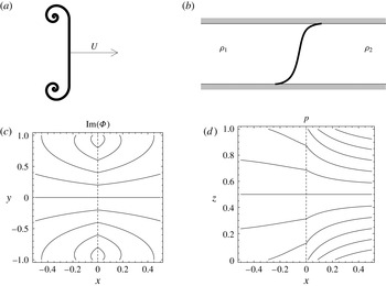
(a,b) Schematic of the initial evolution of the vortex sheet (a) and interface (b) for the Kaffeelöffel and dam-break thought-experiments. (c,d) Level sets of Kaffeelöffel instantaneous streamfunction (c) and dam-break pressure (d) at
 $t=0^{+}$
in the lab frame. Parameters are
 $L=1$
,
 $U=1$
(c), and
 ${\it\rho}_{1}=0.5$
,
 ${\it\rho}_{2}=2$
(d). Only the horizontal strips spanning
 $-1\leqslant y\leqslant 1$
and
 $0\leqslant z\leqslant 1$
, respectively for plate and gate, are depicted, showing the discontinuous derivatives of the isolines of streamfunction (c) and pressure (d) across the vortex sheet and density interface, respectively.

Some mathematical similarities exist between the Kaffeelöffel thought-experiment and a particular realization of the asymptotically static, layered fluids which are the subject of our study. Consider the ‘internal’ dam-break problem for a two-fluid system confined in a channel (see Camassa et al.
Reference Camassa, Chen, Falqui, Ortenzi and Pedroni2013, for details). This setup is defined as an incompressible Euler fluid, initially at rest and under gravity, of density
 ${\it\rho}_{2}$
(resp.
 ${\it\rho}_{1}$
) filling the right side
 $x>0$
(resp. left side
 $x<0$
) of a horizontal channel between horizontal rigid boundaries located at heights
 $z=0,1$
(with
 ${\it\rho}_{2}>{\it\rho}_{1}$
, say). Such a configuration can be achieved with a gate at
 $x=0$
initially separating the two fluids, which is then instantaneously removed or dissolved at time
 $t=0$
. Immediately after the gate removal, the initial horizontal component of the pressure gradient as
 $x\rightarrow 0^{\pm }$
can be computed explicitly,
 $$\begin{eqnarray}\displaystyle \frac{\partial p}{\partial x}(0^{\pm },z)={\it\Upsilon}_{\pm }\log \left(\frac{1+\cos ({\rm\pi}\,z)}{1-\cos ({\rm\pi}\,z)}\right),\quad {\it\Upsilon}_{-}\equiv \frac{g\,{\it\rho}_{1}\,({\it\rho}_{2}-{\it\rho}_{1})}{{\rm\pi}\,({\it\rho}_{2}+{\it\rho}_{1})},\quad {\it\Upsilon}_{+}\equiv \frac{g\,{\it\rho}_{2}\,({\it\rho}_{2}-{\it\rho}_{1})}{{\rm\pi}\,({\it\rho}_{2}+{\it\rho}_{1})}. & & \displaystyle \nonumber\\ \displaystyle & & \displaystyle\end{eqnarray}$$
Thus, at time
 $t=0^{+}$
the pressure gradient jumps across the interface at
 $x=0$
between the two fluids, and diverges at the points (
 $z=0,1$
) where the gate was in contact with the rigid horizontal boundaries. These points, after the gate removal, become the intersections of the interface between the two density layers with the confining boundaries of the fluid. At the same time, and consequently, the fluid acceleration
 $-\boldsymbol{{\rm\nabla}}p/{\it\rho}$
has a continuous horizontal component but suffers a jump, proportional to the density difference, for the vertical component. Thus, the acceleration in the dam-break problem mirrors the continuity properties of the velocity of the Kaffeelöffel case, with continuous normal and discontinuous tangential components in both problems. The pressure for the dam-break case could also be viewed as the counterpart of the streamfunction in the Kaffeelöffel vortex sheet generation: both pressure and streamfunction, respectively for the dam-break and the Kaffeelöffel case, are continuous but suffer jumps in their horizontal gradient components. Moreover, the mathematical singularities in both setups play a similar role, at least initially, in the evolution of vortex sheets. The shear that develops as a consequence of the jump in the vertical component of the pressure gradient for the dam-break (recall that the pressure is continuous at
 $x=0$
) is ‘pulled’ horizontally to the left and right, respectively, for
 $z<1/2$
and
 $z>1/2$
, by the pressure forces exerted on the fluid. These are strongest at the intersection points where the pressure gradient diverges at
 $z=0$
and
 $z=1$
. The result is an S-shaped vortex sheet at the early times of evolution following the gate removal (see Camassa et al.
Reference Camassa, Chen, Falqui, Ortenzi and Pedroni2013, figure 16, for a direct numerical simulation), not unlike the way the initial vortex sheet in the Kaffeelöffel experiment extends (and bends) in response to the singular pressure forces at the plate tips once this is removed. This similarity is illustrated in figure 1. (We remark that the pressure/streamfunction analogy between the dam-break and Kaffeelöffel thought-experiments does not quite hold for times before the removal of the objects, since the pressure jumps across the dam before its removal, while the streamfunction maintains its continuity. Also note that, unlike the dam break setup, the fluid domain for the Kaffeelöffel experiment is the whole plane
 $(x,y)$
.)
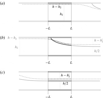
Consequences of the interplay between vorticity balance laws and topological changes of isopycnals in layered flows might also be familiar under a different guise, which we will now briefly sketch in another idealized example. Consider the setup of a gravity current in a two-layer incompressible Euler fluid studied by von Kármán (Reference von Kármán1940) and Benjamin (Reference Benjamin1968), depicted in figure 2, that can be described as follows. In a two-dimensional domain confined between two rigid, horizontal plates, a flat interface at infinity separates the two fluids to the right of the domain. There, the fluid in the upper layer moves to the left with constant horizontal velocity, feeding the advancement from right to left of a point at finite range where the interface contacts the upper plate. For this solution of the Euler equations, the only location of the interface at right-infinity compatible with total horizontal momentum and energy conservation is exactly at the middle of the channel, regardless of the density difference between the two fluids (Benjamin Reference Benjamin1968). Accordingly, the gravity-current front moves from right to left at a constant speed selected by this depth of the interface. If
 $h$
still denotes the vertical distance between the plates and
 $h_{2}^{\prime }$
is the thickness of the lower-layer fluid to the far right of the domain, one has
 $$\begin{eqnarray}h_{2}^{\prime }=h/2,\end{eqnarray}$$
while the asymptotic velocities to the right of the lower and upper fluids are, respectively,
 $u_{2}^{\prime }=c_{0}/2$
and
 $u_{1}^{\prime }=-u_{2}^{\prime }$
, where
 $c_{0}\equiv \sqrt{g\,h\,(1-{\it\rho}_{r})}$
is the critical long-wave speed, with the definition of density ratio
 ${\it\rho}_{r}\equiv {\it\rho}_{1}/{\it\rho}_{2}$
. In contrast, suppose that the interface never contacts the upper plate at finite range but may approach it asymptotically towards infinity to the left. For this setup, a solution of the Euler equations compatible with momentum conservation also exists (see e.g. Choi & Camassa Reference Choi and Camassa1999), and can be interpreted as a limiting case of a so-called conjugate-state solution. In this case, the thickness of the lower-layer fluid to the far right is
 $$\begin{eqnarray}h_{2}^{\prime }=\frac{h}{\sqrt{{\it\rho}_{r}}+1},\end{eqnarray}$$
while the asymptotic velocities are, respectively,
 $u_{2}^{\prime }=c_{0}h_{2}\,/h-c$
and
 $u_{1}^{\prime }=-u_{2}^{\prime }/\sqrt{{\it\rho}_{r}}$
, where
 $c=c_{0}/(1+\sqrt{{\it\rho}_{r}})$
is the velocity of the front, and
 $h_{2}$
is the thickness of the lower fluid at the far left of the channel.
Schematic of gravity-current (solid) and conjugate-state (dash) propagation in a two-layer fluid. A lab-frame observer’s test section is highlighted in the region between
 $-L$
and
 $L$
. Sketches refer to times where the front of either solution with respect to the test section is: (a) approaching from far to the right, (b) moving through, (c) travelling out to the far left, leaving a steady horizontal vortex sheet behind.

In a test section of width
 $2L$
, as either the gravity current or the conjugate-state front moves from the far right to far left (see figure 2), an observer would see the total fluid vorticity increase from zero to a constant value at sufficiently large times. This is because the fluid in the test window is initially at rest, and after the front has moved through, the stratified fluid remains in steady motion with a vortex sheet determined by the velocity jump across the interface, for either the gravity-current or the conjugate-state solutions. As can be seen from the expression of the fluid velocities, at large times the total vorticity in the test section is the same for both gravity currents and the limiting case of conjugate states, that is
 $$\begin{eqnarray}{\it\Gamma}_{w}=2L\sqrt{g\,h\,(1-{\it\rho}_{r})},\end{eqnarray}$$
but, interestingly, the effect of the intersection with the upper wall of the interface between the two fluids causes the abrupt difference between its asymptotic height at large times seen by comparing (2.4) for the gravity current solution versus (2.5) for the conjugate state, respectively, with
 ${\it\rho}_{r}<1$
. Thus, the difference between measurable quantities such as the time-asymptotic location of the interface between the two fluids in the test section can ultimately be attributed to the effect of the topological change of a density isoline.
3. Two-dimensional systems: a unifying perspective on momentum and vorticity conservation laws
We begin by recalling some results obtained in Camassa et al. (Reference Camassa, Chen, Falqui, Ortenzi and Pedroni2012, Reference Camassa, Chen, Falqui, Ortenzi and Pedroni2013) concerning motion in a two-dimensional fluid domain (a channel) of the form
 ${\it\Omega}\equiv \mathbb{R}\times [z_{-},z_{+}]$
. If
 $(x,z)$
and
 $(u,w)$
denote the Cartesian components of coordinates and velocity field, respectively, the total horizontal fluid momentum is
 $$\begin{eqnarray}{\it\Pi}\equiv \int _{{\it\Omega}}{\it\rho}u\,\text{d}x\,\text{d}z.\end{eqnarray}$$
It can be shown that
 ${\it\Pi}$
is not a constant of the motion, since its time-derivative is
 $$\begin{eqnarray}\dot{{\it\Pi}}=-h\langle p\rangle _{{\it\Delta}},\end{eqnarray}$$
where
 $h=z_{+}-z_{-}$
is the channel height and the layer-average
 $\langle p\rangle _{{\it\Delta}}$
of the pressure jump at the channel end-points is
 $$\begin{eqnarray}\langle p\rangle _{{\it\Delta}}\equiv \frac{1}{h}\int _{z_{-}}^{z_{+}}(p(+\infty ,z)-p(-\infty ,z))\,\text{d}z.\end{eqnarray}$$
Moreover, it turns out that
 $\langle p\rangle _{{\it\Delta}}=p(+\infty ,\bar{z})-p(-\infty ,\bar{z})$
for any
 $\bar{z}\in [z_{-},z_{+}]$
, and that this pressure difference is in general non-zero, as already remarked in Benjamin (Reference Benjamin1986) and further substantiated in Camassa et al. (Reference Camassa, Chen, Falqui, Ortenzi and Pedroni2012, Reference Camassa, Chen, Falqui, Ortenzi and Pedroni2013).
In two dimensions the local vorticity
 ${\it\omega}=w_{x}-u_{z}$
is a scalar. The total vorticity
 ${\it\Gamma}$
is
 $$\begin{eqnarray}{\it\Gamma}\equiv \int _{{\it\Omega}}{\it\omega}\,\text{d}x\,\text{d}z=\int _{\mathbb{R}}(u^{-}-u^{+})\,\text{d}x,\end{eqnarray}$$
where
 $f^{\pm }(x,t)\equiv f(x,z_{\pm },t)$
denote, hereafter, the boundary values of the quantity
 $f(x,z,t)$
. By setting
 $\lim _{|x|\rightarrow \infty }{\it\rho}^{+}(x)\equiv {\it\rho}_{1}$
,
 $\lim _{|x|\rightarrow \infty }{\it\rho}^{-}(x)\equiv {\it\rho}_{2}$
, and
 ${\it\rho}_{_{{\it\Delta}}}\equiv {\it\rho}_{2}-{\it\rho}_{1}$
, and by using the horizontal component of the Euler equations, the time-derivative of the total vorticity turns out to be
 $$\begin{eqnarray}\dot{{\it\Gamma}}=\frac{{\it\rho}_{_{{\it\Delta}}}\langle p\rangle _{{\it\Delta}}}{{\it\rho}_{1}{\it\rho}_{2}}+\int _{\mathbb{R}}\left(\frac{{\it\rho}_{x}^{+}}{({\it\rho}^{+})^{2}}p^{+}-\frac{{\it\rho}_{x}^{-}}{({\it\rho}^{-})^{2}}p^{-}\right)\text{d}x.\end{eqnarray}$$
Equations (3.2) and (3.5) suggest the definition of the quantity
 $$\begin{eqnarray}\mathscr{G}\equiv {\it\Gamma}+\frac{{\it\rho}_{_{{\it\Delta}}}}{{\it\rho}_{1}{\it\rho}_{2}h}{\it\Pi},\end{eqnarray}$$
whose time-evolution is
 $$\begin{eqnarray}\dot{\mathscr{G}}=\int _{\mathbb{R}}\left(\frac{{\it\rho}_{x}^{+}}{({\it\rho}^{+})^{2}}\,p^{+}-\frac{{\it\rho}_{x}^{-}}{({\it\rho}^{-})^{2}}\,p^{-}\right)\text{d}x.\end{eqnarray}$$
If the density is constant on the upper and lower lids (i.e. if
 ${\it\rho}^{+}(x)={\it\rho}_{1}$
and
 ${\it\rho}^{-}(x)={\it\rho}_{2}$
for all
 $x$
), then
 $\mathscr{G}$
is a conserved quantity, related to those classified in Benjamin (Reference Benjamin1986) by
 $$\begin{eqnarray}\mathscr{G}=\frac{{\it\rho}_{_{{\it\Delta}}}}{h{\it\rho}_{1}{\it\rho}_{2}}\mathscr{I}+\frac{z_{+}{\it\rho}_{1}-z_{-}{\it\rho}_{2}}{h{\it\rho}_{1}{\it\rho}_{2}}\mathscr{C},\end{eqnarray}$$
where
 $$\begin{eqnarray}\displaystyle \left.\begin{array}{@{}c@{}}\displaystyle \mathscr{C}\equiv \int _{{\it\Omega}}{\it\sigma}~\text{d}x\,\text{d}z=\frac{{\it\Pi}^{-}}{h}-\frac{{\it\Pi}^{+}}{h},\\ \displaystyle \mathscr{I}\equiv \int _{{\it\Omega}}z{\it\sigma}~\text{d}x\,\text{d}z={\it\Pi}-\frac{z_{+}}{h}{\it\Pi}^{+}+\frac{z_{-}}{h}{\it\Pi}^{-},\end{array}\right\} & & \displaystyle\end{eqnarray}$$
with
 ${\it\sigma}\equiv ({\it\rho}w)_{x}-({\it\rho}u)_{z}$
and
 ${\it\Pi}^{\pm }\equiv h\int _{\mathbb{R}}{\it\rho}^{\pm }u^{\pm }\,\text{d}x$
. Because of property (3.7), the quantity
 $\mathscr{G}$
acts as an indicator of the topological features of the pycnocline surfaces with respect to the fluid domain boundaries. We will henceforth refer to
 $\mathscr{G}$
as the ‘topological vorticity’.
As pointed out in Camassa et al. (Reference Camassa, Chen, Falqui, Ortenzi and Pedroni2014), whenever the density at the lids fails to be constant, the determination of the motion invariants (and of the Hamiltonian representation of the system) is substantially altered; in particular, boundary values of all the fields have to be carefully considered. The upshot of such a topological change is that the quantities (3.9) are no longer conserved, since their balance laws are
 $$\begin{eqnarray}\dot{\mathscr{C}}=\mathscr{J}^{+}-\mathscr{J}^{-}\end{eqnarray}$$
and
 $$\begin{eqnarray}\dot{\mathscr{I}}=z_{+}\mathscr{J}^{+}-z_{-}\mathscr{J}^{-},\end{eqnarray}$$
where
 $\mathscr{J}^{\pm }$
are given by
 $$\begin{eqnarray}\mathscr{J}^{\pm }\equiv \frac{1}{2}\int _{-\infty }^{+\infty }{\it\rho}_{\,\,x}^{\pm }(u^{\pm })^{2}\,\text{d}x.\end{eqnarray}$$
The same lack of conservation happens for the topological vorticity
 $\mathscr{G}$
(see (3.7)). We remark that, if the boundary density is not a constant, relation (3.8) should also be modified to
 $$\begin{eqnarray}\mathscr{G}+\frac{1}{{\it\rho}_{1}}\int _{\mathbb{R}}({\it\rho}_{1}-{\it\rho}^{+})\,u^{+}\text{d}x-\frac{1}{{\it\rho}_{2}}\int _{\mathbb{R}}({\it\rho}_{2}-{\it\rho}^{-})\,u^{-}\,\text{d}x=\frac{{\it\rho}_{_{{\it\Delta}}}}{h{\it\rho}_{1}{\it\rho}_{2}}\mathscr{I}+\frac{z_{+}{\it\rho}_{1}-z_{-}{\it\rho}_{2}}{h{\it\rho}_{1}{\it\rho}_{2}}\mathscr{C}.\end{eqnarray}$$
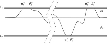
These results become particularly transparent in the simplified case of a sharp two-layer stratification, depicted in figure 3. In this case
 ${\it\rho}^{+}$
(resp.
 ${\it\rho}^{-}$
) can be non-constant only if the lower (resp. upper) fluid touches the upper (resp. lower) boundary. Suppose this happens for
 $x$
in some suitable intervals of the real line; then we can write
 $$\begin{eqnarray}\frac{1}{{\it\rho}^{+}}=\frac{1}{{\it\rho}_{1}}-\frac{{\it\rho}_{_{{\it\Delta}}}}{{\it\rho}_{1}{\it\rho}_{2}}\mathop{\sum }_{i}{\it\chi}_{[{\it\alpha}_{i}^{+},{\it\beta}_{i}^{+}]},\quad \frac{1}{{\it\rho}^{-}}=\frac{1}{{\it\rho}_{2}}+\frac{{\it\rho}_{_{{\it\Delta}}}}{{\it\rho}_{1}{\it\rho}_{2}}\mathop{\sum }_{j}{\it\chi}_{[{\it\alpha}_{j}^{-},{\it\beta}_{j}^{-}]},\end{eqnarray}$$
where the characteristic function
 ${\it\chi}$
is
 ${\it\chi}_{[a,b]}(x)=1$
if
 $x\in [a,b]$
and zero otherwise. Thus, spatial derivatives give rise to Dirac-deltas at the density jumps:
 $$\begin{eqnarray}\displaystyle & \displaystyle \left(\frac{1}{{\it\rho}^{+}}\right)_{x}=\frac{{\it\rho}_{_{{\it\Delta}}}}{{\it\rho}_{1}{\it\rho}_{2}}\mathop{\sum }_{i}({\it\delta}(x-{\it\beta}_{i}^{+})-{\it\delta}(x-{\it\alpha}_{i}^{+})), & \displaystyle\end{eqnarray}$$
 $$\begin{eqnarray}\displaystyle & \displaystyle \left(\frac{1}{{\it\rho}^{-}}\right)_{x}=-\frac{{\it\rho}_{_{{\it\Delta}}}}{{\it\rho}_{1}{\it\rho}_{2}}\mathop{\sum }_{j}({\it\delta}(x-{\it\beta}_{j}^{-})-{\it\delta}(x-{\it\alpha}_{j}^{-})). & \displaystyle\end{eqnarray}$$
 ${\it\Gamma}$
given in (3.5) becomes
 $$\begin{eqnarray}\displaystyle \dot{{\it\Gamma}} & = & \displaystyle \frac{{\it\rho}_{_{{\it\Delta}}}}{{\it\rho}_{1}{\it\rho}_{2}}\left(\langle p\rangle _{{\it\Delta}}-\mathop{\sum }_{i}(p^{+}({\it\beta}_{i}^{+})-p^{+}({\it\alpha}_{i}^{+}))-\mathop{\sum }_{j}(p^{-}({\it\beta}_{j}^{-})-p^{-}({\it\alpha}_{j}^{-}))\right)\nonumber\\ \displaystyle & = & \displaystyle \frac{{\it\rho}_{_{{\it\Delta}}}}{{\it\rho}_{1}{\it\rho}_{2}}\left(\langle p\rangle _{{\it\Delta}}-\mathop{\sum }_{i}P_{{\it\Delta},i}^{+}-\mathop{\sum }_{j}P_{{\it\Delta},j}^{-}\right),\end{eqnarray}$$
where
 $P_{{\it\Delta},i}^{+}\equiv p^{+}({\it\beta}_{i}^{+})-p^{+}({\it\alpha}_{i}^{+})$
and
 $P_{{\it\Delta},j}^{-}\equiv p^{-}({\it\beta}_{j}^{-})-p^{-}({\it\alpha}_{j}^{-})$
are the local boundary pressure differences. These local differences need not vanish in general (an instance of such non-trivial contributions is illustrated in Camassa et al.
Reference Camassa, Chen, Falqui, Ortenzi and Pedroni2013). They are related to the variation of the amount of boundary momentum contained in the intervals
 $[{\it\alpha}_{i}^{\pm },{\it\beta}_{i}^{\pm }]$
by
 $$\begin{eqnarray}\displaystyle P_{{\it\Delta},i}^{+} & = & \displaystyle \int _{{\it\alpha}_{i}^{+}}^{{\it\beta}_{i}^{+}}p_{x}^{+}\,\text{d}x=-\int _{{\it\alpha}_{i}^{+}}^{{\it\beta}_{i}^{+}}{\it\rho}_{2}(u_{t}^{+}+u^{+}u_{x}^{+})\,\text{d}x\nonumber\\ \displaystyle & = & \displaystyle -\dot{{\it\Pi}}_{i}^{+}+{\it\rho}_{2}(u^{+}({\it\beta}_{i}^{+})\dot{{\it\beta}}_{i}^{+}-u^{+}({\it\alpha}_{i}^{+})\dot{{\it\alpha}}_{i}^{+})-\left.{\textstyle \frac{1}{2}}{\it\rho}_{2}(u^{+})^{2}\right|_{{\it\alpha}_{i}^{+}}^{{\it\beta}_{i}^{+}},\end{eqnarray}$$
where
 ${\it\Pi}_{i}^{+}\equiv h\int _{{\it\alpha}_{i}^{+}}^{{\it\beta}_{i}^{+}}{\it\rho}_{2}u^{+}\,\text{d}x$
. Similarly, we obtain
 $$\begin{eqnarray}P_{{\it\Delta},j}^{-}=-\dot{{\it\Pi}}_{j}^{-}+{\it\rho}_{1}(u^{-}({\it\beta}_{j}^{-})\dot{{\it\beta}}_{j}^{-}-u^{-}({\it\alpha}_{j}^{-})\dot{{\it\alpha}}_{j}^{-})-\left.{\textstyle \frac{1}{2}}{\it\rho}_{1}(u^{-})^{2}\right|_{{\it\alpha}_{j}^{-}}^{{\it\beta}_{j}^{-}},\end{eqnarray}$$
where
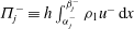 ${\it\Pi}_{j}^{-}\equiv h\int _{{\it\alpha}_{j}^{-}}^{{\it\beta}_{j}^{-}}{\it\rho}_{1}u^{-}\,\text{d}x$
. By using the relations
 $$\begin{eqnarray}\dot{{\it\beta}}_{i}^{\pm }=u^{\pm }({\it\beta}_{i}^{\pm }),\quad \dot{{\it\alpha}}_{i}^{\pm }=u^{\pm }({\it\alpha}_{i}^{\pm }),\end{eqnarray}$$
we can write the local pressure differences as
 $$\begin{eqnarray}P_{{\it\Delta},i}^{+}=-\dot{{\it\Pi}}_{i}^{+}+\left.{\textstyle \frac{1}{2}}{\it\rho}_{2}(u^{+})^{2}\right|_{{\it\alpha}_{i}^{+}}^{{\it\beta}_{i}^{+}},\quad P_{{\it\Delta},j}^{-}=-\dot{{\it\Pi}}_{j}^{-}+\left.{\textstyle \frac{1}{2}}{\it\rho}_{1}(u^{-})^{2}\right|_{{\it\alpha}_{j}^{-}}^{{\it\beta}_{j}^{-}}.\end{eqnarray}$$
Two-dimensional setup: typical interface configuration contributing to total vorticity evolution through boundary terms.

The second and the third terms in (3.17) can be considered as topological contributions to the time-variation of
 ${\it\Gamma}$
. As shown in Camassa et al. (Reference Camassa, Chen, Falqui, Ortenzi and Pedroni2013), if the initial velocities are zero these contributions are proportional to
 ${\it\rho}_{_{{\it\Delta}}}^{2}$
, and can therefore dominate the first term which is proportional to
 ${\it\rho}_{_{{\it\Delta}}}^{3}$
. This can be given the following interpretation. Consider, for simplicity, a sequence of zero-velocity initial fluid configurations in which the lower fluid is arranged with ‘bumps’ whose height grows towards the maximal height
 $z_{+}$
of the upper bounding plate. As long as a sliver of lighter fluid between the upper lid and the top of a bump of heavier fluid is present the initial variation of total vorticity is given by
 $\dot{{\it\Gamma}}={\it\rho}_{_{{\it\Delta}}}\,\langle p\rangle _{{\it\Delta}}/({\it\rho}_{1}{\it\rho}_{2})$
. This quantity varies smoothly with the bump heights. On the other hand, when one or more slivers of upper fluid between bumps and the upper plate disappear, jumps can occur in the time-variation of
 ${\it\Gamma}$
, since this is now given by all the terms in (3.17). Such abrupt changes should be expected to happen for sequences of interface profiles limiting to profiles that intersect either lid, such as those depicted in figure 3.
4. The three-dimensional case: momentum and vorticity balance
Paradoxical results about momentum conservation in stratified, incompressible Euler fluids in unbounded domains emerge due to the interplay between incompressibility and stratification (Benjamin Reference Benjamin1986; Camassa et al.
Reference Camassa, Chen, Falqui, Ortenzi and Pedroni2012, Reference Camassa, Chen, Falqui, Ortenzi and Pedroni2013). The paradoxical nature of these results can be traced back to the effects of incompressibility in homogeneous-density fluids. The classical computation of the total momentum integral over unbounded domains (Saffman Reference Saffman1992; Falkovich Reference Falkovich2011) with localized force distributions shows that the total momentum, and its variation in time, depend conditionally on the limit to infinity of finite volume integrals. While for homogeneous fluids in the two-dimensional case of a channel the limit of infinite volumes does not require handling conditionally convergent integrals, the same setup for inhomogeneous fluids is more delicate, as already pointed out in Benjamin (Reference Benjamin1986) and further discussed in Camassa et al. (Reference Camassa, Chen, Falqui, Ortenzi and Pedroni2012, Reference Camassa, Chen, Falqui, Ortenzi and Pedroni2013). To a larger extent, three-dimensional settings for stratified fluids require addressing the issue of conditional convergence of volume and surface integrals. This should perhaps be expected in the case of localized density distributions away from hydrostatic equilibrium, as these can be viewed as impulsive force sources, thus leading to similar issues as for their three-dimensional homogeneous counterpart. In what follows, unless otherwise specified, we will always use bounded control volumes
 ${\it\Omega}$
and take their unbounded limits to handle the case of infinite channels. Depending on the situation, we will explicitly indicate when such volumes can be taken as material objects, whether by using impermeable walls or by letting them evolve with the fluid motion according to the Lagrangian perspective.
Next, we first briefly review the three-dimensional analogue of the horizontal momentum evolution equation (3.2), and then move on to examine the total vorticity equation (3.5) in three-dimensional settings.
4.1. Three-dimensional momentum and impulse evolution
For a stratified fluid under gravity confined between two rigid infinite horizontal planes the time-derivative of the total horizontal momentum may depend on the shape of the lateral boundary in the limit to infinite domains. For a stratified fluid in three dimensions, this can be seen by suitably reinterpreting the link between total momentum
 $$\begin{eqnarray}{\it\bf\Pi}=\int _{{\it\Omega}}{\rm\pi}\,\text{d}V\equiv \int _{{\it\Omega}}{\it\rho}\boldsymbol{u}\,\text{d}V,\end{eqnarray}$$
and hydrodynamical impulse (in analogy with the two-dimensional case as in Benjamin Reference Benjamin1986),
 $$\begin{eqnarray}\boldsymbol{I}\equiv \frac{1}{2}\int _{{\it\Omega}}\boldsymbol{x}\times {\bf\sigma}\,\text{d}V\,\quad \text{with }{\bf\sigma}\equiv \boldsymbol{{\rm\nabla}}\times ({\it\rho}\boldsymbol{u}),\end{eqnarray}$$
by replacing the velocity vector
 $\boldsymbol{u}$
used in Saffman (Reference Saffman1992) and Falkovich (Reference Falkovich2011) with the momentum vector
 ${\rm\pi}={\it\rho}\boldsymbol{u}$
. Using standard formulae of vector calculus we can write the relation between momentum
 ${\it\bf\Pi}$
and impulse
 $\boldsymbol{I}$
as
 $$\begin{eqnarray}{\it\bf\Pi}=\boldsymbol{I}+\frac{1}{2}\int _{\partial {\it\Omega}}({\it\rho}\boldsymbol{u}(\boldsymbol{n}\boldsymbol{\cdot }\boldsymbol{x})-\boldsymbol{n}({\it\rho}\boldsymbol{u}\boldsymbol{\cdot }\boldsymbol{x}))\text{d}S.\end{eqnarray}$$
Here, following general definitions, see e.g. Saffman (Reference Saffman1992) or Majda & Bertozzi (Reference Majda and Bertozzi2002), we have restored the factor
 $1/2$
in the definition of the impulse, so that its first component is
 $\mathscr{I}/2$
with respect to the definition of the two-dimensional case in the previous section. The last integral in (4.3) is zero for sufficiently fast-decaying velocities at infinity (for instance, if
 ${\it\Omega}$
is a sphere, for velocities decaying faster than
 $r^{-3}$
), but may very well be non-zero in a number of physical solutions of the Euler equations (for homogeneous fluids, numerous examples can be found in Lamb Reference Lamb1932). Moreover, as soon as the velocity field has a non-vanishing dipole moment (and thus the integral on the right-hand side of (4.3) is only conditionally convergent), the surface integral depends on the geometry of the boundary
 $\partial {\it\Omega}$
of the fluid volume
 ${\it\Omega}$
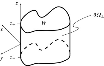
. In the special case of a ‘cylindrical’ shape
 ${\it\Omega}=W\times [z_{-},z_{+}]$
as in figure 4 one gets
 $$\begin{eqnarray}\boldsymbol{I}_{\bot }={\it\bf\Pi}_{\bot }-\frac{z_{+}}{2h}{\it\bf\Pi}_{\bot }^{+}+\frac{z_{-}}{2h}{\it\bf\Pi}_{\bot }^{-}-\frac{1}{2}\int _{\partial {\it\Omega}_{\bot }}((\boldsymbol{n}\boldsymbol{\cdot }\boldsymbol{x}){\it\rho}\boldsymbol{u}_{\bot }-({\it\rho}\boldsymbol{u}\boldsymbol{\cdot }\boldsymbol{x})\boldsymbol{n})\,\text{d}S,\end{eqnarray}$$
where the subscript
 $\bot$
denotes horizontal components of vectors,
 $\partial {\it\Omega}_{\bot }$
is the lateral boundary and, in analogy with the notation of § 3, we define
 $$\begin{eqnarray}{\it\bf\Pi}_{\bot }^{\pm }=h\int _{W}{\rm\pi}_{\bot }(x,y,z_{\pm })\,\text{d}x\,\text{d}y.\end{eqnarray}$$
When the density along the plates
 $z=z_{\pm }$
is constant, and for zero-velocity initial conditions, the time-derivative of the horizontal impulse
 $\boldsymbol{I}_{\bot }$
can be shown to vanish at time
 $t=0$
(with a suitable modification of the arguments presented in e.g. Saffman Reference Saffman1992, for the case of a homogeneous fluid), so that (4.4) yields
 $$\begin{eqnarray}\dot{{\it\bf\Pi}}_{\bot }=\frac{z_{+}}{2h}\,\dot{{\it\bf\Pi}}_{\bot }^{+}-\frac{z_{-}}{2h}\dot{{\it\bf\Pi}}_{\bot }^{-}+\frac{1}{2}\int _{\partial {\it\Omega}_{\bot }}((\boldsymbol{n}\boldsymbol{\cdot }\boldsymbol{x})\,\boldsymbol{{\rm\nabla}}_{\bot }p-(\boldsymbol{{\rm\nabla}}p\boldsymbol{\cdot }\boldsymbol{x})\boldsymbol{n})\,\text{d}S.\end{eqnarray}$$
The last term makes apparent how the geometry of the lateral vertical boundary
 $\partial {\it\Omega}_{\bot }$
explicitly enters the time-variation of the total momentum. Notice that the pressure gradient plays, in the time-variation formula, exactly the same role as played by the (horizontal) momentum
 ${\it\rho}\boldsymbol{u}_{\bot }$
in (4.3). We may expect non-trivial contributions when the dipole moment of the pressure gradient is non-zero, so that the integral on the right-hand side of (4.6) is not absolutely convergent. Some explicit computations of such geometry-dependent contributions are reported in appendix A.
Schematics of cylindrical fluid domains for impulse and momentum time-variations.

We end this section with a remark: while for constant density along the plates in two-dimensional settings the horizontal impulse is always conserved (Benjamin Reference Benjamin1986) as this corresponds to the Noether’s symmetry of horizontal translational invariance, in three dimensions this no longer holds (in general) for stratified fluid between infinite horizontal plates. In particular, (4.6) does not hold beyond initial times, since the term
 $\dot{\boldsymbol{I}}_{\bot }$
is not zero in general. Conservation of horizontal impulse is recovered, for instance, when
 ${\bf\omega}\boldsymbol{\cdot }\boldsymbol{n}=0$
along the plates. The influence of this condition on the vorticity evolution is discussed next.
4.2. Three-dimensional vorticity
The evolution equation for the vorticity in three dimensions is given by
 $$\begin{eqnarray}{\bf\omega}_{t}+(\boldsymbol{u}\boldsymbol{\cdot }\boldsymbol{{\rm\nabla}}){\bf\omega}-{\bf\omega}\boldsymbol{\cdot }\boldsymbol{{\rm\nabla}}\boldsymbol{u}+\boldsymbol{{\rm\nabla}}\times \left(\frac{\boldsymbol{{\rm\nabla}}p}{{\it\rho}}\right)=0.\end{eqnarray}$$
In the absence of vortex sheets, this implies that the time-variation of the total fluid vorticity is
 $$\begin{eqnarray}\dot{{\it\bf\Gamma}}=-\int _{\partial {\it\Omega}}(\boldsymbol{u}\boldsymbol{\cdot }\boldsymbol{n}){\bf\omega}\,\text{d}S+\int _{\partial {\it\Omega}}({\bf\omega}\boldsymbol{\cdot }\boldsymbol{n})\boldsymbol{u}\,\text{d}S-\int _{{\it\Omega}}\boldsymbol{{\rm\nabla}}\times \left(\frac{\boldsymbol{{\rm\nabla}}p}{{\it\rho}}\right)\text{d}V.\end{eqnarray}$$
With either a material interpretation or with wall boundary conditions for the control volume
 ${\it\Omega}$
, the first transport term on the right-hand side of this equation would be absent. This property would be preserved in time for the case of a homogeneous fluid, as a consequence of Kelvin circulation invariance. The second and third terms on the right-hand side of expression (4.8) can be naturally classified as the kinematic and baroclinic terms, denoted respectively by
 $\dot{{\it\bf\Gamma}}_{kin}$
and
 $\dot{{\it\bf\Gamma}}_{bar}$
. With a material surface defined by
 ${\bf\omega}\boldsymbol{\cdot }\boldsymbol{n}=0$
at some instant in time, the second (kinematic) term would also be absent from the right-hand side of (4.8). While in general both the kinetic and baroclinic terms contribute to the variation of total vorticity (as already remarked by Poincaré Reference Poincaré1893), we shall henceforth concentrate on the latter to show how the topology of velocity and density discontinuities play a fundamental role in the variation of the total vorticity.
The consequences of non-trivial stratifications, giving rise to the baroclinic term in (4.8), are the focus of this section. First, we study the more intuitive case of a sharp two-layer stratification in a cylindrically shaped domain
 ${\it\Omega}=W\times [z_{-},z_{+}]$
. In this setting, as we shall see, the topological aspects emerge in a particularly transparent way.
4.2.1. The two-layer case
In the two-layer case the density, and possibly the tangent component of the velocity, are discontinuous at the interface
 $z={\it\eta}(x,y,t)$
between the two fluids. In particular, we have
 $$\begin{eqnarray}{\it\rho}={\it\rho}_{2}-{\it\rho}_{{\it\Delta}}H(z-{\it\eta}(x,y,t)),\end{eqnarray}$$
where we are maintaining the notation of § 3, i.e.
 ${\it\rho}_{2}$
(resp.
 ${\it\rho}_{1}$
) is the density of the lower (resp. upper) fluid,
 ${\it\rho}_{_{{\it\Delta}}}={\it\rho}_{2}-{\it\rho}_{1}$
, and
 $H$
is the Heaviside function.
To compute the baroclinic contribution of the total vorticity evolution
 $$\begin{eqnarray}\dot{{\it\bf\Gamma}}_{bar}=-\int _{{\it\Omega}}\boldsymbol{{\rm\nabla}}\times \left(\frac{\boldsymbol{{\rm\nabla}}p}{{\it\rho}}\right)\text{d}V,\end{eqnarray}$$
we need to carefully interpret the curl in the distributional sense owing to the fact that the density has a jump along the interface
 ${\it\Sigma}$
between the two fluids. This leads to
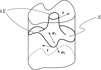
 $$\begin{eqnarray}\dot{{\it\bf\Gamma}}_{bar}=-\int _{{\it\Sigma}}\boldsymbol{n}_{1}\times \left(\frac{\boldsymbol{{\rm\nabla}}p_{1}}{{\it\rho}_{1}}\right)\text{d}S-\int _{{\it\Sigma}}\boldsymbol{n}_{2}\times \left(\frac{\boldsymbol{{\rm\nabla}}p_{2}}{{\it\rho}_{2}}\right)\text{d}S,\end{eqnarray}$$
where
 $p_{1}$
(resp.
 $p_{2}$
) is the pressure in the upper (resp. lower) layer, and
 $\boldsymbol{n}_{1}$
(resp.
 $\boldsymbol{n}_{2}$
) is the unit normal to
 ${\it\Sigma}$
pointing to the upper (resp. lower) layer. By standard theorems of vector calculus (see e.g. Smirnov Reference Smirnov1964, p. 322) we obtain
 $$\begin{eqnarray}\dot{{\it\bf\Gamma}}_{bar}=\frac{1}{{\it\rho}_{1}}\int _{\partial {\it\Sigma}}p_{1}\boldsymbol{t}\,\text{d}l-\frac{1}{{\it\rho}_{2}}\int _{\partial {\it\Sigma}}p_{2}\boldsymbol{t}\,\text{d}l,\end{eqnarray}$$
where the tangent vector
 $\boldsymbol{t}$
is oriented according to the rule that it lead to counterclockwise circulation along
 $\partial {\it\Sigma}$
with respect to the normal
 $\boldsymbol{n}_{2}$
(see e.g. figure 5). Continuity of the pressure yields the final formula
 $$\begin{eqnarray}\dot{{\it\bf\Gamma}}_{bar}=\frac{{\it\rho}_{_{{\it\Delta}}}}{{\it\rho}_{1}{\it\rho}_{2}}\int _{\partial {\it\Sigma}}p\boldsymbol{t}\,\text{d}l.\end{eqnarray}$$
If we denote by
 ${\it\gamma}_{{\it\alpha}}$
the connected components of the interface
 ${\it\Sigma}$
, we obviously have
 $$\begin{eqnarray}\dot{{\it\bf\Gamma}}_{bar}=\frac{{\it\rho}_{_{{\it\Delta}}}}{{\it\rho}_{1}{\it\rho}_{2}}\mathop{\sum }_{{\it\alpha}}\int _{{\it\gamma}_{{\it\alpha}}}p\boldsymbol{t}_{{\it\alpha}}\,\text{d}l_{{\it\alpha}},\end{eqnarray}$$
where the tangent vector is oriented according to the rule that ‘a – long-armed and short-legged – walker upright in the direction of the outward normal to
 $\partial {\it\Omega}$
, and moving along the loop
 ${\it\gamma}_{{\it\alpha}}$
according to the orientation set by
 $\boldsymbol{t}_{{\it\alpha}}$
, would keep the left-hand immersed in the heavier fluid’.
A simple case of a two-layer configuration with a topologically non-trivial interface.

In most applications of (4.14), the pycnocline will intersect the lateral boundary
 $\partial {\it\Omega}_{\bot }$
along a closed loop
 ${\it\gamma}_{_{\infty }}$
, and it is convenient to single out the corresponding term in (4.14) so that it reads
 $$\begin{eqnarray}\dot{{\it\bf\Gamma}}_{bar}=\frac{{\it\rho}_{_{{\it\Delta}}}}{{\it\rho}_{1}{\it\rho}_{2}}\int _{{\it\gamma}_{_{\infty }}}p\boldsymbol{t}_{\infty }\,\text{d}l_{\infty }+\frac{{\it\rho}_{_{{\it\Delta}}}}{{\it\rho}_{1}{\it\rho}_{2}}\mathop{\sum }_{{\it\beta}}\int _{{\it\gamma}_{{\it\beta}}}p\boldsymbol{t}_{{\it\beta}}\,\text{d}l_{{\it\beta}}.\end{eqnarray}$$
It is natural to denote the second term as the ‘topological contribution’ to
 $\dot{{\it\bf\Gamma}}_{bar}$
, as it keeps track of the topology of the pycnocline deformations of this surface, as illustrated in figure 6.
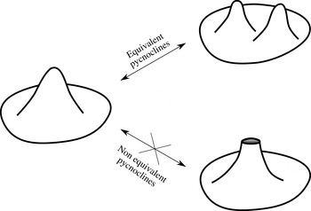
Two-layer system: sketch of possible interface topologies. Each interface ‘hole’ contributes a term to the evolution of total vorticity. The shape of the hole boundary, and not the contact angle, is the only interface feature affecting the baroclinic term of vorticity evolution.

Two remarks are in order. First, note that this formula does not carry any information on the way the interface between the two fluids intersects the boundary of the domain
 ${\it\Omega}$
. In particular, angles of intersection do not play a role in the final expression (4.14). Second, the sign choice in (4.14) agrees with the two-dimensional case (3.17), taking into account that
 ${\it\Gamma}=-{\it\bf\Gamma}\boldsymbol{\cdot }\boldsymbol{j}$
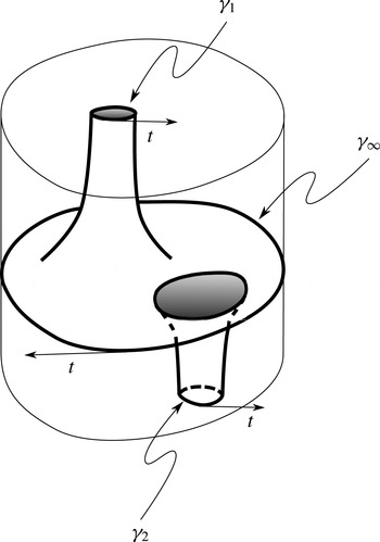
. To see this, consider the setup depicted in figure 7: both top and bottom circuits between the two fluids end up being oriented counterclockwise for an upright observer viewing the channel from above.
Two-layer system: orientations of top and bottom circuits of the interface intersections with horizontal boundaries.

Let us now define the three-dimensional analogue of the topological vorticity
 $\mathscr{G}$
introduced in § 3 (for a specific class of fluid domains
 ${\it\Omega}$
and interface configurations as graphs over the horizontal variables
 $z={\it\eta}(x,y,t)$
). This vector topological vorticity is given by
 $$\begin{eqnarray}\mathbf{\mathscr{G}}\equiv {\it\bf\Gamma}+\frac{{\it\rho}_{_{{\it\Delta}}}}{h{\it\rho}_{1}{\it\rho}_{2}}{\it\bf\Pi}\times \boldsymbol{k},\end{eqnarray}$$
and its time-evolution can be computed as follows. As can be readily shown, the time-variation of the total horizontal momentum of the fluid filling
 ${\it\Omega}$
is given by
 $$\begin{eqnarray}\dot{{\it\bf\Pi}}_{\bot }=\int _{{\it\Omega}}\frac{\partial }{\partial t}({\it\rho}\boldsymbol{u}_{\bot })\,\text{d}V=-\int _{\partial {\it\Omega}_{\bot }}{\it\rho}\boldsymbol{u}_{\bot }\,(\boldsymbol{u}\boldsymbol{\cdot }\boldsymbol{n})\,\text{d}S-\int _{\partial {\it\Omega}_{\bot }}p\boldsymbol{n}\,\text{d}S.\end{eqnarray}$$
Let us suppose that the base
 $W$
of the domain
 ${\it\Omega}$
is sufficiently large that the hydrostatic condition on pressure can be applied asymptotically at
 $\partial {\it\Omega}_{\bot }$
,
 $$\begin{eqnarray}\left.p_{j}|_{\partial {\it\Omega}_{\bot }}\sim -{\it\rho}_{j}g(z-{\it\eta})\right|_{\partial {\it\Omega}_{\bot }}+\,P|_{{\it\gamma}_{_{\infty }}},\quad j=1,2,\end{eqnarray}$$
where
 $P$
is the interfacial pressure. (That the pressure
 $p$
can be asymptotic to a non-constant value due to the directional dependence of
 $P$
, even under the limiting hydrostatic assumption, might not be immediately clear; a few explicit examples will be provided in appendix A.) Further, we assume that horizontal velocity goes to zero sufficiently fast (for a dipole term it would be
 $O(|\boldsymbol{x}_{\bot }|^{-3})$
) so that the transport term in (4.17) can be neglected, and that the interface between the two fluids be asymptotically horizontal, as appropriate for hydrostatic equilibria. This means that
 ${\it\eta}$
is a constant (
 ${\it\eta}=z_{0}$
, say) on the lateral vertical boundary of
 ${\it\Omega}$
, so that the intersection curve
 ${\it\gamma}_{_{\infty }}$
is horizontal, i.e.
 $\boldsymbol{t}_{\infty }\boldsymbol{\cdot }\boldsymbol{k}=0$
. We obtain
 $$\begin{eqnarray}\dot{{\it\bf\Pi}}_{\bot }=-\int _{\partial {\it\Omega}_{\bot }}(P-{\it\rho}g(z-{\it\eta}))\boldsymbol{n}\,\text{d}S=-\int _{\partial {\it\Omega}_{\bot }}P\boldsymbol{n}\,\text{d}S.\end{eqnarray}$$
Since
 $\boldsymbol{t}_{\infty }=\boldsymbol{n}\times \boldsymbol{k}$
, taking the cross-product with
 $\boldsymbol{k}$
we get
 $$\begin{eqnarray}\dot{{\it\bf\Pi}}\times \boldsymbol{k}=\dot{{\it\bf\Pi}}_{\bot }\times \boldsymbol{k}=-\int _{\partial {\it\Omega}_{\bot }}P\boldsymbol{t}_{\infty }\,\text{d}S=-h\int _{{\it\gamma}_{_{\infty }}}P\boldsymbol{t}_{\infty }\,\text{d}l,\end{eqnarray}$$
where
 $l$
is the arc length parameter of
 ${\it\gamma}_{_{\infty }}$
. Similarly to the two-dimensional case, when the density is constant along the upper and lower lids (so that the pycnocline does not intersect either of the bounding channel plates) it follows from the baroclinic vorticity variation defined by (4.14) that the evolution of
 $\mathbf{\mathscr{G}}$
is simply
 $$\begin{eqnarray}\dot{\mathbf{\mathscr{G}}}=\dot{{\it\bf\Gamma}}_{kin}.\end{eqnarray}$$
For the special surfaces
 $\partial {\it\Omega}$
defined by
 ${\bf\omega}\boldsymbol{\cdot }\boldsymbol{n}=0$
, which in the channel case can imply
 ${\bf\omega}\boldsymbol{\cdot }\boldsymbol{k}=0$
along the plates, the right-hand side of this relation would vanish for the velocity class we are considering (decaying at infinity as
 $O(1/|\boldsymbol{x}_{\bot }|^{3})$
), so that
 $\mathbf{\mathscr{G}}$
turns out to be a constant of the motion.
Conversely, let us now consider topologically non-trivial situations, where the pycnocline intersects the upper or lower lids along some closed curves, and hence coincides with the rigid plates in the regions internal to these curves. In this case, (4.21) becomes
 $$\begin{eqnarray}\dot{\mathbf{\mathscr{G}}}=\dot{{\it\bf\Gamma}}_{kin}+\frac{{\it\rho}_{_{{\it\Delta}}}}{{\it\rho}_{1}{\it\rho}_{2}}\mathop{\sum }_{{\it\beta}}\int _{{\it\gamma}_{{\it\beta}}}p\boldsymbol{t}_{{\it\beta}}\,\text{d}l_{{\it\beta}},\end{eqnarray}$$
where the sum is taken over the top and bottom intersection curves (thus excluding the limiting
 ${\it\gamma}_{_{\infty }}$
defined above along the lateral boundary of
 ${\it\Omega}$
), i.e. the curves defined by
 ${\it\eta}(x,y)=z_{+}$
and
 ${\it\eta}(x,y)=z_{-}$
. Note that the vertical component of
 $\dot{\mathbf{\mathscr{G}}}$
is not affected by the contributions from the contours
 ${\it\gamma}_{{\it\beta}}$
, unlike its horizontal components.
Equation (4.22) conveys the topological contribution to the balance law for
 $\mathbf{\mathscr{G}}$
due to non-trivial pycnocline configurations generating non-simply connected interfaces between the two fluids.
4.2.2. Continuous stratifications
The topological effects studied above for two-layer configurations extend directly to the more physically relevant case of continuous stratifications, whenever the density fails to be constant along the bounding horizontal lids. The baroclinic term of the
 ${\it\bf\Gamma}$
evolution is now
 $$\begin{eqnarray}\dot{{\it\bf\Gamma}}_{bar}=-\int _{{\it\Omega}}\boldsymbol{{\rm\nabla}}\times \left(\frac{\boldsymbol{{\rm\nabla}}p}{{\it\rho}}\right)\text{d}V=\int _{\partial {\it\Omega}}p\boldsymbol{n}\times \boldsymbol{{\rm\nabla}}\left(\frac{1}{{\it\rho}}\right)\text{d}S.\end{eqnarray}$$
Therefore, in the cylindrical geometry we are considering,
 $\dot{{\it\bf\Gamma}}_{bar}$
can be split into three different components,
 $$\begin{eqnarray}\dot{{\it\bf\Gamma}}_{bar}=\int _{\partial {\it\Omega}_{\bot }}p\boldsymbol{n}\times \boldsymbol{{\rm\nabla}}\left(\frac{1}{{\it\rho}}\right)\text{d}S-\int _{W}p\boldsymbol{k}\times \boldsymbol{{\rm\nabla}}\left.\left(\frac{1}{{\it\rho}}\right)\right|_{z_{-}}\text{d}S+\int _{W}p\boldsymbol{k}\times \boldsymbol{{\rm\nabla}}\left.\left(\frac{1}{{\it\rho}}\right)\right|_{z_{+}}\text{d}S,\end{eqnarray}$$
where the second and third terms on the right-hand side are evaluated at the top and bottom plates
 $z=z_{\pm }$
. Note that these two terms vanish when
 ${\it\rho}$
is constant along the plates. For most applications, all isopycnals can be assumed to intersect the lateral boundary
 $\partial {\it\Omega}_{\bot }$
along closed curves as the domain
 $W$
limits to infinity, since the fluid will be assumed to be in isotropic hydrostatic equilibrium at infinity. Thus, the terms in (4.24) are the counterpart for continuously stratified fluids of those in (4.15); in particular, the first term can be viewed as the continuous version of the first term (4.15), while the second and third terms constitute the topological contribution from density isopycnals intersecting the bounding plates at
 $z=z_{\pm }$
.
Despite their similarity with the layered case, continuous stratifications do require some care in handling the integrals at the top and lower lids in (4.24) whenever the density varies along the lids. In fact, let us assume that some isopycnal surfaces have non-trivial intersections with the upper (lower) lid. Typically, such intersections would foliate the lid into a family of closed curves, which can be viewed as ‘holes’ in the isopycnal surface itself. (Not all such curves are necessarily smooth and/or simple, as ‘separatrix’-like configurations can be envisioned to happen.)
Under these circumstances, the topological terms in (4.24) can be computed as follows. Define
 $$\begin{eqnarray}\dot{{\it\bf\Gamma}}_{bar}^{\pm }\equiv \pm \int _{W}p\boldsymbol{k}\times \boldsymbol{{\rm\nabla}}\left.\left(\frac{1}{{\it\rho}}\right)\right|_{z_{\pm }}\text{d}S=\pm \int _{W}\frac{p^{\pm }}{({\it\rho}^{\pm })^{2}}\boldsymbol{T}_{\pm }\,\text{d}x\,\text{d}y,\end{eqnarray}$$
where
 $$\begin{eqnarray}\boldsymbol{T}_{\pm }\equiv \boldsymbol{{\rm\nabla}}{\it\rho}^{\pm }\times \boldsymbol{k}=(({\it\rho}^{\pm })_{y},-({\it\rho}^{\pm })_{x},0)\,\end{eqnarray}$$
is a tangent vector to the curves of constant density on the lids. For simplicity, we focus on the upper lid
 $z=z_{+}$
, and assume a non-constant smooth distribution
 ${\it\rho}(x,y,z_{+})\equiv {\it\rho}^{+}(x,y)$
, with
 ${\it\rho}^{+}(x,y)={\it\rho}_{1}$
on the boundary of
 $W$
. Let us also assume that
 ${\it\rho}^{+}$
has only one critical point in
 $W$
, with critical value
 ${\it\rho}_{max}>{\it\rho}_{1}$
. Then all curves of constant density on the upper plate are closed and bounded. By a change of variables from Cartesian to isopycnal coordinates
 $(x,y)\mapsto ({\it\rho}^{+},l)$
, such that
 $l$
is the arc length parameter on such curves, we get, by taking into account that the Jacobian
 ${\it\rho}_{x}l_{y}-{\it\rho}_{y}l_{x}$
equals
 $\sqrt{{\it\rho}_{x}^{2}+{\it\rho}_{y}^{2}}$
,
 $$\begin{eqnarray}\dot{{\it\bf\Gamma}}_{bar}^{+}=\int _{W}\frac{p^{+}}{({\it\rho}^{+})^{2}}\boldsymbol{T}_{+}\,\text{d}x\,\text{d}y=\int _{{\it\rho}_{1}}^{{\it\rho}_{max}}\left(\oint \frac{p^{+}}{({\it\rho}^{+})^{2}}\boldsymbol{t}_{+}\,\text{d}l\right)\text{d}{\it\rho}^{+},\end{eqnarray}$$
where
 $\boldsymbol{t}_{+}=(x_{l},y_{l})$
is the normalized tangent vector. If the function
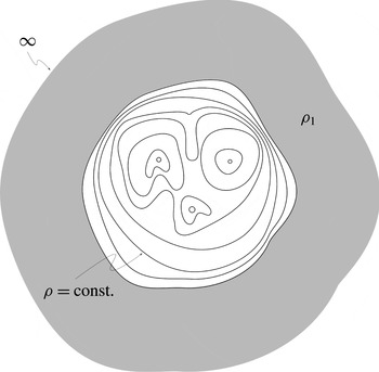
 ${\it\rho}^{+}$
has more than one critical point, as in figure 8, every critical point will provide a similar contribution to the time-variation of the total vorticity. The same argument applies to the lower lid.
A typical density configuration at the upper boundary of the fluid. A similar configuration can exist for the lower boundary with asymptotic density
 ${\it\rho}_{2}$
.

The analogue of the topological vorticity vector
 $\mathbf{\mathscr{G}}$
for continuous stratifications can be defined with an identical expression in terms of the vorticity
 ${\it\bf\Gamma}$
and the total momentum
 ${\it\bf\Pi}$
to that of the two-layer case (4.16). Perhaps surprisingly, the time-variations of
 $\mathbf{\mathscr{G}}$
reduce to the same expressions as those for the two-layer case under natural assumptions. In fact, under asymptotic isotropic hydrostatic equilibrium at infinity,
 ${\it\rho}(\boldsymbol{x},t)\rightarrow {\it\rho}_{\infty }(z)$
, and for velocities whose asymptotic decay guarantees the vanishing of the first term on the right-hand side of (4.17) (e.g. in a cylindrical geometry,
 $\boldsymbol{u}_{\bot }$
decaying faster than
 $|\boldsymbol{x}_{\bot }|^{-1/2}$
would suffice), the time-derivative of the total momentum yields
 $$\begin{eqnarray}\dot{{\it\bf\Pi}}\times \boldsymbol{k}=-\int _{\partial {\it\Omega}_{\bot }}p\boldsymbol{n}\times \boldsymbol{k}\,\text{d}S=-\int _{\partial {\it\Omega}_{\bot }}p\boldsymbol{t}_{\infty }\,\text{d}S=-\int _{\partial {\it\Omega}_{\bot }}(P(l)+r(z))\boldsymbol{t}_{\infty }\,\text{d}S.\end{eqnarray}$$
Here, for the last term we have used the asymptotic property of the pressure (see appendix A for the case of zero initial velocities) which implies
 $$\begin{eqnarray}p(\boldsymbol{x},t)\sim P(l,t)-g\int ^{z}{\it\rho}_{\infty }(s)\,\text{d}s\equiv P(l,t)+r(z)\quad \text{as}~\boldsymbol{x}_{\bot }\rightarrow \infty .\end{eqnarray}$$
In (4.28) the second term vanishes, as
 $$\begin{eqnarray}\int _{\partial {\it\Omega}_{\bot }}r(z)\boldsymbol{t}_{\infty }\,\text{d}S=\left(\int _{z_{-}}^{z_{+}}r(z)\,\text{d}z\right)\left(\oint _{\partial W}\boldsymbol{t}_{\infty }\,\text{d}l\right)=0,\end{eqnarray}$$
since the integral of the unit tangent vector along its loop vanishes. Hence,
 $$\begin{eqnarray}\dot{{\it\bf\Pi}}\times \boldsymbol{k}=-\oint _{\partial W}P(l)\boldsymbol{t}_{\infty }\,\text{d}l\,\int _{z_{-}}^{z_{+}}\text{d}z=-h\oint _{\partial W}P(l)\boldsymbol{t}_{\infty }\,\text{d}l.\end{eqnarray}$$
This expression matches its two-layer counterpart (4.20), upon observing that for the present configuration
 ${\it\gamma}_{\infty }$
is the rigid translation of the boundary of the plate domain
 $\partial W$
.
When the density is constant along the upper and lower plates (namely,
 ${\it\rho}(x,y,z_{+})={\it\rho}_{1}$
and
 ${\it\rho}(x,y,z_{-})={\it\rho}_{2}$
) and the fluid is asymptotically in isotropic equilibrium at infinity, performing similar manipulations with the baroclinic vorticity time-variation, equation (4.10) yields
 $$\begin{eqnarray}\dot{{\it\bf\Gamma}}_{bar}=\oint _{\partial W}P(l)\boldsymbol{t}_{\infty }\,\text{d}l\,\int _{z_{-}}^{z_{+}}\left(\frac{1}{{\it\rho}}\right)_{z}\text{d}z\,=\frac{{\it\rho}_{_{{\it\Delta}}}}{{\it\rho}_{1}{\it\rho}_{2}}\oint _{\partial W}P(l)\boldsymbol{t}_{\infty }\,\text{d}l.\end{eqnarray}$$
Here again we have used the null property of the integral of the tangent for cancelling the term
 $$\begin{eqnarray}\left(\oint _{\partial W}\boldsymbol{t}_{\infty }\,\text{d}l\right)\left(\int _{z_{-}}^{z_{+}}r(z)\left(\frac{1}{{\it\rho}}\right)_{z}\text{d}z\right)\end{eqnarray}$$
which arises in the computation. The time-derivative
 $\dot{{\it\bf\Gamma}}_{bar}$
is thus
 $$\begin{eqnarray}\dot{{\it\bf\Gamma}}_{bar}=-\frac{{\it\rho}_{_{{\it\Delta}}}}{h{\it\rho}_{1}{\it\rho}_{2}}\dot{{\it\bf\Pi}}\times \boldsymbol{k},\end{eqnarray}$$
just as in the two-layer case. Hence,
 $$\begin{eqnarray}\dot{\mathbf{\mathscr{G}}}=\dot{{\it\bf\Gamma}}_{kin}\end{eqnarray}$$
still holds for the continuously stratified case, under the assumptions we have made. As before, for the non-trivial topology of isopycnals outlined above, the evolution of the topological vorticity
 $\mathbf{\mathscr{G}}$
acquires the topological contribution to the total vorticity (4.27), since the evolution of the momentum
 ${\it\bf\Pi}$
with continuous stratification remains unaffected by the topology.
5. The case of a free surface
Finally, we briefly discuss how the previous results are modified by removing the constraint of a rigid lid and replacing it with a free surface at
 $z={\it\eta}(x,y,t)$
, with constant pressure
 $p=p_{a}$
. Even if pycnoclines can intersect the free boundary, there are now substantial dynamical differences between the topological contributions to the vorticity time-evolution with respect to rigid horizontal boundaries.
For the free-boundary case the interpretation of the control volume
 $$\begin{eqnarray}{\it\Omega}=\{(x,y,z)\mid (x,y)\in W,~z_{-}<z<{\it\eta}(x,y,t)\}\end{eqnarray}$$
is naturally Lagrangian. Similarly to rigidly bounded fluids, the time-derivative of the total vorticity can still be split into its kinematic and baroclinic components, with the latter defined in (4.23) as
 $$\begin{eqnarray}\dot{{\it\bf\Gamma}}_{bar}=-\int _{{\it\Omega}}\boldsymbol{{\rm\nabla}}\times \left(\frac{\boldsymbol{{\rm\nabla}}p}{{\it\rho}}\right)\text{d}V=\int _{\partial {\it\Omega}}p\boldsymbol{n}\times \boldsymbol{{\rm\nabla}}\left(\frac{1}{{\it\rho}}\right)\text{d}S.\end{eqnarray}$$
Therefore
 $$\begin{eqnarray}\dot{{\it\bf\Gamma}}_{bar}=\int _{\partial {\it\Omega}_{\bot }}p\boldsymbol{n}\times \boldsymbol{{\rm\nabla}}\left(\frac{1}{{\it\rho}}\right)\text{d}S+\int _{z={\it\eta}}p\boldsymbol{n}_{{\it\eta}}\times \boldsymbol{{\rm\nabla}}\left(\frac{1}{{\it\rho}}\right)\text{d}S-\int _{z=z_{-}}p\boldsymbol{k}\times \boldsymbol{{\rm\nabla}}\left(\frac{1}{{\it\rho}}\right)\text{d}S,\end{eqnarray}$$
where the free-surface integral must be identically zero, since clearly the arbitrary constant in the definition of pressure cannot contribute to the vorticity time-variation. This can be seen directly by the same change of variables as used in (4.27) from Cartesian to isopycnal coordinates. In the cylindrical domain of the previous section we have applied this change of variables at the fixed upper lid, while now it must be applied to the time-varying free surface of the fluid. Denoting by
 ${\it\rho}^{+}$
the fluid density at the free surface, the interface baroclinic contribution to the vorticity evolution is
 $$\begin{eqnarray}\int _{z={\it\eta}}p\boldsymbol{n}_{{\it\eta}}\times \boldsymbol{{\rm\nabla}}\left(\frac{1}{{\it\rho}}\right)\text{d}S=-p_{a}\int _{{\it\rho}_{1}}^{{\it\rho}_{max}}\frac{1}{({\it\rho}^{+})^{2}}\left(\oint \boldsymbol{t}_{+}\,\text{d}l\right)\text{d}{\it\rho}^{+}=0,\end{eqnarray}$$
where the last equality holds because the circulation of the tangent vector along a closed curve is zero. The first term in (5.3) is the non-topological contribution already encountered in the rigid-lid case of the previous section, and vanishes for fluids asymptotically in hydrostatic equilibrium. However, unlike the rigid-lid case, the constant-pressure boundary condition kills the topological contribution from the top, leaving only the isopycnal topology at the bottom to give a possibly non-zero contribution. The free-surface contribution to vorticity is therefore purely kinematical, due to the fact that the normal velocity to the free surface may not be identically zero.
6. Conclusions
Inspired by well-known results on the dynamics of gravity currents (von Kármán Reference von Kármán1940; Benjamin Reference Benjamin1968) and by the conceptual problems posited by the thought-experiment of Klein’s Kaffeelöffel, in this work we have studied the implications of certain density configurations on conservation laws for the motion of stratified incompressible Euler fluids in infinite domains. Specifically, we have shown that the localized intersections of density isoclines with the rigid boundaries contribute additional source terms, determined by the topology of the intersections, to the evolution of the fluid total vorticity, much as the change of topology of vortex sheets can contribute to the vorticity evolution for a homogeneous fluid in Klein’s example.
After a review of the two-dimensional case, stemming from our earlier investigations, we have focused here on three-dimensional setups. These place additional challenges with respect to their two-dimensional counterparts, in that the convergence for infinite domains of integrals of certain physical quantities, such as momentum and vorticity, is of more fundamental nature in three dimensions and needs to be interpreted carefully, as partially seen already for homogeneous incompressible fluid flows.
The essential features of our results can be most simply seen in the ideal case of a two-layer fluid between two infinite rigid plates. When the pycnocline remains separated from the plates, the evolution of the total vorticity due to the baroclinic term essentially mirrors that of the horizontal momentum due to asymptotic interfacial pressure imbalances. However, when pycnocline intersections with the plates occur, the vorticity evolution acquires additional forcing terms with respect to that of momentum; these are mathematically represented in (4.15) by the loop integrals along the localized intersection curves. These loop integrals, in turn, collect the contributions of local pressure imbalances along the plates. Remarkably, the total momentum balance is not affected by these local terms, and their effect remains confined to the total vorticity evolution. This leads to the definition of the ‘topological vorticity’ vector
 $\mathbf{\mathscr{G}}$
, whose dynamic evolution originates in these local intersection terms. The topological vorticity balance generalizes to the more physically relevant case of continuously stratified fluids, and leads to similar source terms (4.27) once isopycnal coordinates along the plates are used.
Some of the consequences of the topological effects we have discussed seem to deserve further attention. For instance, as in the case of the Kaffeelöffel experiment, topological changes such as those caused by reconnections would require the presence of other physical mechanisms with respect to the ones we have studied, for instance the diffusivity of stratifying agents such as heat or salt, which can affect the slope of pycnoclines at contact points along boundaries, as in the experiment by Phillips (Reference Phillips1970). Of course, for real immiscible fluids, surface tension can also be expected to play a role. Finally, the presence of a (possibly mild) viscosity as in the experiments by Wibawa et al. (Reference Wibawa, Steele, Dahl, Rival, Weymouth and Triantafyllou2012) would have to be included for modelling real fluids, specially at longer time scales. In the absence of these additional physical properties, a certain isopycnal topology in an evolving geometry could persist at all finite times throughout the fluid evolution. This can pose a challenge for the development of models, such as those based on long-wave approximations, as the underlying asymptotic assumptions may become invalid during their time-evolution. Some of these issues will be examined in future work.
Acknowledgements
We thank A. Della Vedova for discussions and useful comments on different aspects of this paper. This work was carried out under the auspices of the GNFM Section of INdAM. Partial support by NSF grants DMS-1009750, RTG DMS-0943851 and CMG ARC-1025523, as well as by the MIUR Cofin2010–2011 project 2010JJ4KPA is acknowledged. R.C. and M.P. thank the Dipartimento di Matematica e Applicazioni of Università Milano-Bicocca for its hospitality. In addition, ETH Zurich and the Fields Institute (R.C.) are gratefully acknowledged for their hospitality while some of this work was being carried out. Last, but not least, we would like to thank the anonymous referees for bringing the interesting paper by Wibawa et al. (Reference Wibawa, Steele, Dahl, Rival, Weymouth and Triantafyllou2012) to our attention and for their careful reading of the manuscript which helped improve the exposition.
Appendix A. Momentum balance for continuously stratified fluids
As is well known, incompressibility leads to an elliptic problem of Poisson type for the pressure in the Euler equations of stratified fluids. This requires boundary conditions to be specified, which for infinite fluid domains can lead to conditionally convergent integrals for Green-type identities. In this section we consider specific examples of two geometric domains under the simplifying assumption of vanishing initial velocities, and take advantage of a perturbative technique for small density differences to derive explicit expressions for the pressure. More general setups with non-zero velocities can be dealt with by similar techniques; however, the case of zero initial velocities highlights the effects of even small density stratifications in balance laws such as that of momentum.
Recall from Camassa et al. (Reference Camassa, Chen, Falqui, Ortenzi and Pedroni2013) that for small
 ${\it\rho}_{_{{\it\Delta}}}$
the solution to the pressure equation
 $$\begin{eqnarray}\boldsymbol{{\rm\nabla}}\boldsymbol{\cdot }\left(\frac{1}{{\it\rho}}\boldsymbol{{\rm\nabla}}p\right)=0,\end{eqnarray}$$
for zero initial velocity with hydrostatic boundary conditions, can be sought in the form of an asymptotic expansion
 $$\begin{eqnarray}p=p^{(0)}+{\it\epsilon}p^{(1)}+{\it\epsilon}^{2}p^{(2)}+\cdots\end{eqnarray}$$
in the small parameter
 ${\it\epsilon}$
defined by
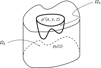
 $$\begin{eqnarray}{\it\rho}(x,y,z)={\it\rho}_{b}(z)-{\it\epsilon}{\it\rho}^{\prime }(x,y,z),\quad 0<{\it\epsilon}\ll 1.\end{eqnarray}$$
Thus,
 ${\it\rho}^{\prime }(x,y,z)$
is a (localized) perturbation to a background hydrostatic equilibrium density
 ${\it\rho}_{b}(z)$
, and
 ${\it\epsilon}$
measures the non-dimensional magnitude of the density difference. The steps for determining each term in the asymptotic expansion in three-dimensional settings are essentially equivalent to those in two dimensions carried out in Camassa et al. (Reference Camassa, Chen, Falqui, Ortenzi and Pedroni2013), and most of the details can be skipped here; the main difference lies in the form of the Green’s function for a three-dimensional, as opposed to two-dimensional, volume.
The hierarchy of equations that determine the pressure at each order of the asymptotic expansion yields, at second order,
 $$\begin{eqnarray}\boldsymbol{{\rm\nabla}}\boldsymbol{\cdot }\left(\frac{1}{{\it\rho}_{b}}\boldsymbol{{\rm\nabla}}\,p^{(2)}\right)=-\boldsymbol{{\rm\nabla}}\boldsymbol{\cdot }\left(\frac{{\it\rho}^{\prime }}{{\it\rho}_{b}^{2}}\,\boldsymbol{{\rm\nabla}}p^{(1)}+\frac{{\it\rho}^{\prime 2}}{{\it\rho}_{b}^{3}}\boldsymbol{{\rm\nabla}}p^{(0)}\right)\equiv F.\end{eqnarray}$$
The boundary conditions will of course depend on the particular setup for the fluid domain
 ${\it\Omega}$
. In general, a portion of the boundary
 $\partial {\it\Omega}$
will be fixed while the rest will limit to infinity. For instance, for an infinite pipe of square cross-section, the domain is
 ${\it\Omega}=\mathbb{R}\times [0,1]\times [0,1]$
, and the boundary conditions on the pressure
 $p^{(2)}$
read
 $$\begin{eqnarray}\left.\frac{\partial p^{(2)}}{\partial z}\right|_{z=0,1}=\left.\frac{\partial p^{(2)}}{\partial y}\right|_{y=0,1}=0,\quad \frac{\partial p^{(2)}}{\partial x}\rightarrow 0\quad \text{as}~|x|\rightarrow \infty .\end{eqnarray}$$
The consistency of the right-hand side
 $F$
with the boundary conditions for
 $p^{(2)}$
can be verified in general and ultimately relies on the assumption of hydrostatic equilibrium at infinity for the system.
Consider the Green’s function
 $G$
for the operator
 $u\mapsto \boldsymbol{{\rm\nabla}}\boldsymbol{\cdot }((1/{\it\rho}_{b})\boldsymbol{{\rm\nabla}}u)$
. The Green’s identity, which we write as
 $$\begin{eqnarray}p^{(2)}(\boldsymbol{x})=\int _{\partial {\it\Omega}}\left(\frac{p^{(2)}({\bf\xi})}{{\it\rho}_{b}({\it\zeta})}\,\frac{\partial G}{\partial \boldsymbol{n}_{{\it\xi}}}(\boldsymbol{x}|{\bf\xi})-\,\frac{\partial p^{(2)}}{\partial \boldsymbol{n}_{{\it\xi}}}({\bf\xi})\,\frac{G(\boldsymbol{x}|{\bf\xi})}{{\it\rho}_{b}({\it\zeta})}\right)\text{d}S_{{\it\xi}}+\int _{{\it\Omega}}G(\boldsymbol{x}|{\bf\xi})\,F({\bf\xi})\,\text{d}V_{{\it\xi}},\end{eqnarray}$$
expresses the solution to (A 4) at a point
 $\boldsymbol{x}\in {\it\Omega}$
in terms of the boundary data and lower-order terms absorbed in the function
 $F({\bf\xi})$
.
A practical application of (A 6) will be exemplified in two particular cases below. In both setups, we shall make the assumption that the functional dependence on
 ${\bf\xi}$
of the integrand is such that in the limit of infinite
 $\partial {\it\Omega}$
the boundary integral
 $$\begin{eqnarray}\int _{\partial {\it\Omega}}\left(\frac{p^{(2)}({\bf\xi})}{{\it\rho}_{b}({\it\zeta})}\,\frac{\partial G}{\partial \boldsymbol{n}_{{\it\xi}}}(\boldsymbol{x}|{\bf\xi})-\,\frac{\partial p^{(2)}}{\partial \boldsymbol{n}_{{\it\xi}}}({\bf\xi})\,\frac{G(\boldsymbol{x}|{\bf\xi})}{{\it\rho}_{b}({\it\zeta})}\right)\text{d}S_{{\it\xi}}\end{eqnarray}$$
remains well defined, and evaluates to a constant independent of the way the boundary
 $\partial {\it\Omega}$
limits to infinity (according to some scale
 $L$
, say). Owing to the pressure indeterminacy up to constants, we will carry out the calculation for
 $p^{(2)}({\bf\xi})$
in these two particular cases ignoring this constant, and verify a posteriori that the solution is compatible with this assumption. Solution uniqueness (up to constants) will then guarantee that the expression for
 $p^{(2)}(\boldsymbol{x})$
thus obtained is the correct one for (A 4). Furthermore, in both examples, we will assume that the support of
 $F({\bf\xi})$
is compact,
 ${\it\Omega}_{L^{\prime }}$
say, with a typical length scale
 $L^{\prime }\ll L$
. This can always be achieved by assuming that the perturbation density
 ${\it\rho}^{\prime }(\boldsymbol{x})$
dependence is appropriately confined (see figure 9). Under these circumstances, the well-known moment expansion of the Green’s function applies to the appropriate free-space component of
 $G(\boldsymbol{x}|{\bf\xi})$
, which for constrained cases refers to the lower-dimensional projection of the portion of fluid domain which can limit to infinity.
Sketch of a typical support
 ${\it\Omega}_{L}^{\prime }$
for the density perturbation
 ${\it\rho}^{\prime }(x,y,z)$
; in the complement domain
 ${\it\Omega}_{L}\!\setminus \!{\it\Omega}_{L}^{\prime }$
the fluid density
 ${\it\rho}_{b}(z)$
depends only on the vertical coordinate
 $z$
.

We are now in position to discuss our two examples of the Green’s function moment expansion which are relevant for the fluid setup we have studied in the body of the paper. We will deal with a two-layer fluid, with densities
 ${\it\rho}_{2}=1$
and
 ${\it\rho}_{1}=1-{\it\epsilon}$
, and we will suppose that the domain of the lighter fluid is bounded, so that we can take
 ${\it\rho}_{b}(z)={\it\rho}_{2}=1$
in the previous formulae, and
 $F({\bf\xi})$
is compactly supported. In this case
 $G$
is the usual Green’s function for the Laplace operator.
A.1. The infinite pipe
Let us first consider the case of a three-dimensional two-layer fluid filling a pipe of square section, of length
 $2L$
with respect to the unit-scale set by the side. Since the projection of the fluid domain that can limit to infinity is one-dimensional, the free-space component
 $G_{0}$
generating the multipole expansion will enter the Green’s function as follows:
 $$\begin{eqnarray}G(\boldsymbol{x}|{\bf\xi})\equiv G_{0}(\boldsymbol{x}|{\bf\xi})+G_{1}(\boldsymbol{x}|{\bf\xi})={\textstyle \frac{1}{2}}|x-{\it\xi}|+G_{1}(\boldsymbol{x}|{\bf\xi}),\end{eqnarray}$$
where
 $\boldsymbol{x}\equiv (x,y,z)$
and
 ${\bf\xi}\equiv ({\it\xi},{\it\eta},{\it\zeta})$
, with boundary conditions
 $$\begin{eqnarray}\left.\frac{\partial G_{1}}{\partial z}\right|_{z=0,1}=\left.\frac{\partial G_{1}}{\partial y}\right|_{y=0,1}=0,\quad \left|\frac{\partial G_{1}}{\partial x}\right|\rightarrow 0\quad \text{as }|x|\rightarrow \infty .\end{eqnarray}$$
Here
 $G_{1}$
is the zero-layer-average component, i.e.
 $\int _{0}^{1}\int _{0}^{1}G_{1}(\boldsymbol{x}|{\bf\xi})\,\text{d}y\,\text{d}z=0,$
which for the boundary conditions (A 9) can be expressed by the Fourier series
 $$\begin{eqnarray}G_{1}=\mathop{\sum }_{n,k=1}^{\infty }g_{nk}(x|{\it\xi})\cos (n{\rm\pi}y)\cos (n{\rm\pi}{\it\eta})\cos (n{\rm\pi}z)\cos (n{\rm\pi}{\it\zeta}),\end{eqnarray}$$
with coefficients
 $g_{nk}$
given by
 $$\begin{eqnarray}g_{nk}(x|{\it\xi})=\frac{1}{2{\rm\pi}\sqrt{n^{2}+k^{2}}}\text{exp}\left(-{\rm\pi}\sqrt{n^{2}+k^{2}}\,|x-{\it\xi}|\right).\end{eqnarray}$$
(In what follows, the most important property of the coefficients
 $g_{nk}$
is the rapid decay at infinity.)
With
 ${\it\rho}_{b}({\it\zeta})=1$
,
 $|x|\gg L$
, and
 $|{\it\xi}|<L$
fixed, the asymptotic expansion of the volume integral in (A 6) then follows by the dominant contribution from the
 $\boldsymbol{x}_{\bot }$
-independent component of the Green’s function
 $G_{0}$
, as
 $$\begin{eqnarray}\displaystyle & |x-{\it\xi}|=|x|-\text{sgn}(x){\it\xi}, & \displaystyle\end{eqnarray}$$
 $$\begin{eqnarray}\displaystyle & \displaystyle p^{(2)}(\boldsymbol{x})\sim \frac{1}{2}|x|\int _{{\it\Omega}_{L}}F({\bf\xi})\,\text{d}V_{{\it\xi}}-\frac{1}{2}\text{sgn}(x)\int _{{\it\Omega}_{L}}{\it\xi}\,F({\bf\xi})\,\text{d}V_{{\it\xi}}, & \displaystyle\end{eqnarray}$$
 ${\it\Omega}_{L}=[-L,L]\times [0,1]\times [0,1]$
. The first volume integral is zero owing to the definition (A 4) of
 $F$
(and the consistency condition of the Poisson equation with Neumann boundary conditions), while the second volume integral defines the dipole moment
 ${\it\mu}$
of the distribution
 $F$
. Hence the asymptotic expression for the pressure at
 $O({\it\epsilon}^{2})$
is
 $$\begin{eqnarray}p^{(2)}(\boldsymbol{x})\sim -\frac{\text{sgn}(x)}{2}\,{\it\mu}.\end{eqnarray}$$
This result is consistent with neglecting the boundary integral contribution in (A 6). Furthermore, this asymptotic formula shows that the time-derivative of horizontal momentum in the direction parallel to the pipe,
 $$\begin{eqnarray}{\it\Pi}_{x}\equiv \int _{-L}^{L}\int _{0}^{1}\int _{0}^{1}{\it\rho}u\,\text{d}x\,\text{d}y\,\text{d}z,\end{eqnarray}$$
is non-zero in general, as
 $$\begin{eqnarray}\left.\dot{{\it\Pi}}_{x}=-\int _{0}^{1}\int _{0}^{1}\,p\right|_{-L}^{L}\text{d}y\,\text{d}z\sim {\it\epsilon}^{2}{\it\mu}.\end{eqnarray}$$
The dipole moment
 ${\it\mu}$
can be expressed explicitly from (A 4),
 $$\begin{eqnarray}{\it\mu}=\int _{{\it\Omega}_{L}}{\it\rho}^{\prime }(\boldsymbol{x})\frac{\partial p^{(1)}}{\partial x}\,\text{d}V.\end{eqnarray}$$
This closely resembles the analogous result for the two-dimensional case (Camassa et al.
Reference Camassa, Chen, Falqui, Ortenzi and Pedroni2013), and can be further reduced to a functional of the initial density distribution
 ${\it\rho}^{\prime }(\boldsymbol{x})$
with the use of the Green’s function expression determining
 $p^{(1)}(\boldsymbol{x})$
from
 ${\it\rho}^{\prime }(\boldsymbol{x})$
.
A.2. The infinite cylinder
As a second example, let us consider a cylindrical domain
 ${\it\Omega}_{L}=D_{L}\times [0,1]$
, where by
 $D_{L}$
we denote the disk of radius
 $L$
. The general arguments at the beginning of this appendix hold, provided we replace the boundary conditions (A 5) with
 $$\begin{eqnarray}\left.\frac{\partial p^{(2)}}{\partial z}\right|_{z=0,1}=0,\quad \frac{\partial p^{(2)}}{\partial \boldsymbol{x}_{\bot }}\rightarrow 0\quad \text{as}~|\boldsymbol{x}_{\bot }|\rightarrow \infty ,\end{eqnarray}$$
where
 $\boldsymbol{x}\equiv (x,y,z)$
and
 $\boldsymbol{x}_{\bot }\equiv (x,y)$
. We can now write a suitable Green’s function as
 $$\begin{eqnarray}G(\boldsymbol{x}|{\bf\xi})\equiv G_{0}(\boldsymbol{x}|{\bf\xi})+G_{1}(\boldsymbol{x}|{\bf\xi})=\frac{1}{2{\rm\pi}}\log |\boldsymbol{x}_{\bot }-{\bf\xi}_{\bot }|+G_{1}(\boldsymbol{x}|{\bf\xi}),\end{eqnarray}$$
where
 ${\bf\xi}\equiv ({\it\xi},{\it\eta},{\it\zeta})$
and
 ${\bf\xi}_{\bot }\equiv ({\it\xi},{\it\eta})$
. Here the zero-layer-average component
 $G_{1}$
of the Green’s function,
 $$\begin{eqnarray}\int _{0}^{1}G_{1}(\boldsymbol{x}|{\bf\xi})\,\text{d}z=0,\end{eqnarray}$$
for the boundary conditions
 $$\begin{eqnarray}\left.\frac{\partial G_{1}}{\partial z}\right|_{z=0,1}=0\end{eqnarray}$$
can be expressed by the Fourier series
 $$\begin{eqnarray}G_{1}=\mathop{\sum }_{n=1}^{\infty }g_{n}(\boldsymbol{x}_{\bot }|{\bf\xi}_{\bot })\cos (n{\rm\pi}z)\cos (n{\rm\pi}{\it\zeta})\end{eqnarray}$$
with the Fourier coefficients
 $g_{n}$
given by
 $$\begin{eqnarray}g_{n}(\boldsymbol{x}_{\bot }|{\bf\xi}_{\bot })=-\frac{1}{2{\rm\pi}}K_{0}(n{\rm\pi}|\boldsymbol{x}_{\bot }-{\bf\xi}_{\bot }|),\end{eqnarray}$$
 $K_{0}$
being the modified Bessel function of the second kind. As for the infinite pipe, the coefficients
 $g_{n}$
are rapidly decaying at infinity. The lateral boundary conditions on
 $G$
are
 $$\begin{eqnarray}\boldsymbol{{\rm\nabla}}G\rightarrow 0\quad \text{as }\boldsymbol{x}_{\bot }\rightarrow \infty .\end{eqnarray}$$
The asymptotic expansion of the volume integral in (A 6), as
 $r\equiv |\boldsymbol{x}_{\bot }|\gg L$
with
 ${\it\rho}_{b}({\it\zeta})=1$
, then follows from that of
 $$\begin{eqnarray}\displaystyle |\boldsymbol{x}_{\bot }-{\bf\xi}_{\bot }| & = & \displaystyle \sqrt{(x-{\it\xi})^{2}+(y-{\it\eta})^{2}}\equiv (r^{2}+{\it\varrho}^{2}-2\boldsymbol{x}_{\bot }\boldsymbol{\cdot }{\bf\xi}_{\bot })^{1/2}\nonumber\\ \displaystyle & = & \displaystyle r\left(1-\frac{\boldsymbol{x}_{\bot }\boldsymbol{\cdot }{\bf\xi}_{\bot }}{r^{2}}+O\left(\frac{{\it\varrho}^{2}}{r^{2}}\right)\right),\end{eqnarray}$$
where we have introduced the cylindrical polar coordinate
 ${\it\varrho}\equiv |{\bf\xi}_{\bot }|$
for the evaluation point’s radial distance from the origin. The dominant contribution to the asymptotics
 $r\gg L$
now comes from the
 $z$
-independent component of the Green’s function
 $G_{0}$
,
 $$\begin{eqnarray}p^{(2)}(\boldsymbol{x})\sim r\int _{{\it\Omega}_{L}}F({\bf\xi})\,\text{d}V_{{\it\xi}}-\frac{\boldsymbol{x}_{\bot }}{r^{2}}\boldsymbol{\cdot }\int _{{\it\Omega}_{L}}{\bf\xi}_{\bot }\,F({\bf\xi})\,\text{d}V_{{\it\xi}}+O\left(\frac{1}{r^{2}}\right).\end{eqnarray}$$
Once again, the first volume integral is zero owing to the definition (A 4) of
 $F$
(and the consistency condition of the Poisson equation with Neumann boundary conditions), while the second volume integral again defines the dipole moment
 ${\bf\mu}$
of the distribution
 $F$
. Hence the asymptotic expression for the pressure at
 $O({\it\epsilon}^{2})$
is
 $$\begin{eqnarray}p^{(2)}(\boldsymbol{x})\sim -\frac{\boldsymbol{x}_{\bot }\boldsymbol{\cdot }{\bf\mu}}{r^{2}}.\end{eqnarray}$$
This result is still consistent with neglecting the boundary integral contribution in (A 6). In particular, the time-derivative of horizontal momentum in the direction set by
 ${\bf\mu}$
,
 $$\begin{eqnarray}{\it\Pi}_{{\it\mu}}\equiv \frac{{\bf\mu}}{|{\bf\mu}|}\boldsymbol{\cdot }\int _{{\it\Omega}_{L}}{\it\rho}\boldsymbol{u}\,\text{d}V,\end{eqnarray}$$
is non-zero in general, as
 $$\begin{eqnarray}\dot{{\it\Pi}}_{{\it\mu}}=-\int _{\partial {\it\Omega}_{L}}\frac{{\bf\mu}\boldsymbol{\cdot }\boldsymbol{n}}{|{\bf\mu}|}\,p\text{d}S\sim {\it\epsilon}^{2}\int _{\partial {\it\Omega}_{L}}\frac{({\bf\mu}\boldsymbol{\cdot }\boldsymbol{n})({\bf\mu}\boldsymbol{\cdot }\boldsymbol{x}_{\bot })}{{\it\mu}\,r^{2}}\,\text{d}S=-{\it\mu}\,{\it\epsilon}^{2}\int _{0}^{2{\rm\pi}}\cos ^{2}{\it\theta}\,\text{d}{\it\theta}=-{\rm\pi}{\it\epsilon}^{2}{\it\mu},\end{eqnarray}$$
where we have set
 $|{\bf\mu}|\equiv {\it\mu}$
. As expected, note that at this order in the asymptotic expansion only the dipole moment contributes to the non-conservation of momentum, due to the decay of all the higher moments of the distribution
 $F$
of order
 $|\boldsymbol{x}_{\bot }|^{-2}$
or faster, which prevents these terms from contributing non-zero boundary integrals as
 ${\it\Omega}_{L}$
limits to infinity. When applied to finite containers with cylindrical symmetry, where constraint horizontal forces clearly prevent momentum conservation, this result shows that momentum evolution can in fact occur first along a direction set by the initial data. Note that this is in addition to possible evolution due to the container shape.