


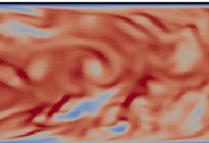





1. Introduction
Inertial particles in wall-bounded flows and their interaction with turbulence and coherent structures have long been investigated both experimentally and numerically. One of the key effects of inertia is that it prevents particles from following highly turbulent motion, which leads to preferential concentration. This was observed for the first time in the numerical simulations by Squires & Eaton (Reference Squires and Eaton1991), and it is sometimes referred to as the particle centrifuge effect. Another important phenomenon of inertial particles in wall-bounded flows is turbophoresis, which denotes the transport of particles from the bulk of the flow to the near-wall region; see Caporaloni et al. (Reference Caporaloni, Tampieri, Trombetti and Vittori1975) and Reeks (Reference Reeks1983). Gravity also affects particle movement and deposition; this has been investigated numerically in Uijttewaal & Oliemans (Reference Uijttewaal and Oliemans1996), Marchioli, Picciotto & Soldati (Reference Marchioli, Picciotto and Soldati2007), Nilsen, Andersson & Zhao (Reference Nilsen, Andersson and Zhao2013) and experimentally among others in Oliveira, Van Der Geld & Kuerten (Reference Oliveira, Van Der Geld and Kuerten2017) and Fong, Amili & Coletti (Reference Fong, Amili and Coletti2019). More information on particle transport in turbulent flows can be found in the review papers by Balachandar & Eaton (Reference Balachandar and Eaton2010) and Brandt & Coletti (Reference Brandt and Coletti2022).
The predominant method to simulate particle-laden flows is based on Lagrangian tracking of a very large number of point particles. The equation of motion of Maxey & Riley (Reference Maxey and Riley1983) is integrated and momentum is exchanged between the two phases. The interaction can be one-way (very dilute suspensions), two-way (relatively low volume fraction, but high mass loading) or four-way coupled (dense suspensions in terms of volume fraction). For low-inertia particles with Stokes number based on the Kolmogorov scale,  $St_k \lessapprox 1$, Eulerian formulations are also applicable (see figure 1 in Balachandar & Eaton Reference Balachandar and Eaton2010) that solve separate momentum and concentration equations for the particulate phase (two-fluid approach); see Guha (Reference Guha2008) and Fox, Laurent & Massot (Reference Fox, Laurent and Massot2008). For particles with even smaller inertia,
 $St_k \lessapprox 0.2\unicode{x2013}0.6$, the equilibrium Eulerian model is applicable. The model is formally derived from the particle equation of motion using Taylor series expansion in terms of
 $St_k$, see Maxey (Reference Maxey1987), Druzhinin (Reference Druzhinin1994) and Ferry & Balachandar (Reference Ferry and Balachandar2001) for a more general form.
The equilibrium Eulerian model, when applicable, is computationally more efficient and easier to implement compared with the Lagrangian approach since it requires only the local flow velocity field and its derivatives to compute the particle velocity. It can also accommodate more easily polydisperse distributions compared with full Eulerian models, and can capture the turbophoresis effect that is known to lead to preferential particle concentration near the wall, see Balachandar & Eaton (Reference Balachandar and Eaton2010) for details. The equilibrium Eulerian model has been applied to both laminar and turbulent flows. For example, Pilou et al. (Reference Pilou, Tsangaris, Neofytou, Housiadas and Drossinos2011) analysed the deposition of inertial particles in a  $90^\circ$ pipe bend for a laminar flow, Icardi et al. (Reference Icardi, Marchisio, Chidambaram and Fox2013) simulated polydisperse particles in a turbulent channel flow using large eddy simulations (LES), Cerminara, Esposti Ongaro & Berselli (Reference Cerminara, Esposti Ongaro and Berselli2016) examined a volcanic ash plume using LES, Yang et al. (Reference Yang, Chen, Socolofsky, Chamecki and Meneveau2016) analysed bubbles in a jet using LES, Aiyer et al. (Reference Aiyer, Yang, Chamecki and Meneveau2019) simulated oil droplets in a cross-flow jet and, finally, Balachandar et al. (Reference Balachandar, Zaleski, Soldati, Ahmadi and Bourouiba2020) suggested this as a method to simulate host-to-host airborne transmission of Covid-19 to establish social distancing guidelines.
The description of particulate flows in an Eulerian framework opens new directions of analysis wherein tools that have been developed for single-phase flows can be directly applied to two-phase flows. In this context, proper orthogonal decomposition (POD) and extended POD were applied recently to characterise the concentration field of low-inertial particles inside turbulent pipe flow (Schlander, Rigopoulos & Papadakis Reference Schlander, Rigopoulos and Papadakis2024). A new Fukagata–Iwamoto–Kasagi identity was also derived to quantify the rate of particle deposition on the pipe wall, and terms that arise due to the effect of turbophoresis appeared naturally.
In the present paper, we consider the application of resolvent analysis for two-phase flows. This is an equation-driven approach, where the governing equations of the fluctuations are Fourier transformed in time (and also space if there are homogeneous directions) and put into an input (forcing)-output (response) form. The nonlinear terms act as forcing to the system. The fluctuations are defined with respect to a time-average field, which is considered known. A singular value decomposition (SVD) is performed on the resolvent operator that relates the input to the output in the frequency domain. The SVD provides the most amplified response modes and the corresponding forcing shapes. In the presence of shear, for example in wall-bounded flows, the operator is low rank (in the sense that the first singular value is orders of magnitude larger than the rest). This feature can be exploited to derive a compact description of the underlying fluctuation field which can be used to provide a low-order representation of the key dynamical processes of turbulence. This approach was proposed by McKeon & Sharma (Reference McKeon and Sharma2010) for single-phase incompressible flows and since then has proven to be a useful framework to probe and analyse turbulent shear flows, see the review of McKeon (Reference McKeon2017) for more details. Most importantly, the resolvent operator can be derived analytically and this allows the derivation of new scaling relations directly from the governing equations, see for example Moarref et al. (Reference Moarref, Sharma, Tropp and McKeon2013). This approach has been extended to supersonic boundary layers (Ahmed et al. Reference Ahmed, Bae, Thompson and McKeon2021), control applications (Luhar, Sharma & McKeon Reference Luhar, Sharma and McKeon2014; Yeh & Taira Reference Yeh and Taira2019) and flow estimation (Thomareis & Papadakis Reference Thomareis and Papadakis2018; Morra et al. Reference Morra, Semeraro, Henningson and Cossu2019; Martini et al. Reference Martini, Cavalieri, Jordan, Towne and Lesshafft2020; Towne, Lozano-Durán & Yang Reference Towne, Lozano-Durán and Yang2020). The statistics of the forcing term were investigated in Morra et al. (Reference Morra, Nogueira, Cavalieri and Henningson2021).
In the above context, the central aim of this paper is to derive the resolvent operator for a turbulent flow laden with low-inertia particles and analyse the effects of inertia and gravity on particle behaviour. For simplicity, we use the Eulerian equilibrium model to obtain the particle velocity field. We explore questions such as, is the resolvent operator low rank? Can it predict particle clustering? What additional physical insight it can bring to explain the effect of inertia and gravity on the particle concentration and its spectra?
Looking at the bigger picture, there is an even more important question to consider. The Eulerian equilibrium model is valid only for low-inertia particles with  $St_k \lessapprox 0.2\unicode{x2013}0.6$. Can the resolvent framework (which is based on an Eulerian description of the flow) be applied to larger particles, where only Lagrangian simulations provide accurate results? In other words, can we bridge the two descriptions? We believe that the answer to the above questions is yes, and we provide some thoughts on this at the end of the paper.
The article is structured as follows: the modelling approach, cases examined (including validation) and mean concentration characteristics are presented in §§ 2–4, respectively. The resolvent operator is derived in § 5 and results are presented in § 6. We summarise the main findings of the paper and discuss directions for future research in § 7.
2. Modelling of turbulent flow with low-inertia particles
We consider the turbulent flow inside a circular pipe with low-inertia particles injected at the inlet. The flow is assumed to be incompressible and the mass fraction of the particles is very small, i.e. the suspension is dilute and the presence of the particles does not affect the flow (one-way coupling). The continuity and momentum equations therefore take the standard form and can be written in Cartesian tensor notation as
 \begin{gather} \frac{\partial u_{i}}{\partial x_{i}} =0, \end{gather}
 \begin{gather}\frac{\partial u_{i}}{\partial t}+ \frac{\partial u_{i}u_{j}}{\partial x_{j}} ={-} \frac{\partial p}{\partial x_{i}}+\frac{1}{Re} \frac{\partial^{2} u_{i}}{\partial x_{j} \partial x_{j}}, \end{gather}
where  $u_i$ is the instantaneous fluid velocity in the
 $i$th direction,
 $p$ is the pressure and
 $t$ is the time. The notation
 $(x_1,x_2,x_3)$ for the spatial coordinates is used interchangeably with the notation
 $(x,y,z)$, where
 $z=x_3$ is the axial (streamwise) direction. Due to rotational symmetry, it is also convenient to use polar coordinates
 $(r,\theta,z)$, where
 $(x,y)=(r \cos \theta,r \sin \theta )$. Velocities are non-dimensionalised with the bulk velocity
 $U_B$, and distances with the pipe diameter
 $D$. The Reynolds number is defined as
 $Re={U_B D}/{\nu }$, where
 $\nu$ is the kinematic viscosity. The mean, i.e. time-average, and fluctuating quantities are denoted by an overbar and a prime, respectively, for example,
 $\overline {u_i}$ and
 $u'_i$.
Eulerian theories for particle deposition in turbulent flows have been proposed; see Guha (Reference Guha1997) and Young & Leeming (Reference Young and Leeming1997) and refer also to Guha (Reference Guha2008) for a review. The theories are based on the formulation of partial differential equations for the momentum and continuity equations for the particle phase. In order to simplify the resulting system, here, we obtain the particle velocity field explicitly from the fluid velocity using the equilibrium Eulerian model of Ferry & Balachandar (Reference Ferry and Balachandar2001). The model is briefly described below; more details are provided in the aforementioned reference.
We assume that the diameter of the particles is much smaller than the Kolmogorov length scale and there are no inter-particle collisions. Furthermore, it is assumed that Stokes drag and gravity are the only forces acting on the particles. Under these conditions, the equation of motion becomes
 \begin{equation} \frac{\mathrm{D} v_i^*}{\mathrm{D} t^*}=\frac{1}{\tau}(u_i^*-v_i^*)+g_i,\end{equation}
where  $t^*$ is the dimensional time,
 ${{\rm D}}/{{\rm D}t^*}$ is the derivative along the particle trajectory,
 $u_i^*$,
 $v_i^*$,
 $g_i$ are the dimensional fluid velocity, particle velocity and gravitational acceleration in the
 $i$th direction, respectively. The particle relaxation time,
 $\tau$, is defined as
 \begin{equation} \tau=\frac{\rho_{\mathrm{p}} d_p^{2}}{18 \mu_f},\end{equation}
where  $\rho _p$,
 $d_p$ are the particle density and diameter, respectively, and
 $\rho _f$,
 $\mu _f$ are the fluid density and dynamic viscosity, respectively. In the present simulations, we take
 $\rho _p/\rho _f \approx 1000$. If
 $\tau$ is small,
 $v_i^*$ can be expanded in Taylor series as (see Maxey Reference Maxey1987)
 \begin{equation} v_i^*=v_i^{(0)}+v_i^{(1)}\tau+v_i^{(2)}\tau^2+\cdots.\end{equation}
Substituting in (2.2), equating terms with the same order of  $\tau$ and retaining only the linear term we arrive at
 \begin{equation} v_i^*=u_i^*-\tau\left(\frac{\mathrm{D} u_i^*}{\mathrm{D} t^*}-g_i\right).\end{equation}
This expression implies that the particle velocity field  $v_i^*(\boldsymbol {x},t)$ is unique and continuous, and it is determined solely by the fluid velocity and its derivatives. Incidentally, the same result can also be obtained from (2.2) assuming that the particle and velocity accelerations are approximately equal. For small enough
 $\tau$, the effect of initial conditions (that results in non-unique solutions) can be neglected because it decays exponentially. The exact condition under which this is satisfied is derived in Ferry & Balachandar (Reference Ferry and Balachandar2001). More complicated expressions that account for other forces in the equation of motion and include quadratic terms in the expansion can be found in Ferry & Balachandar (Reference Ferry and Balachandar2001). For the purposes of the current investigation, however, (2.5) suffices.
The particle concentration  $c^*(\boldsymbol {x},t)$ is defined as the volume of particles per unit volume of fluid; this is also a continuous field. The transport equation for
 $c^*(\boldsymbol {x},t)$ is
 \begin{equation} \frac{\partial c^*}{\partial t^*}+ \frac{\partial v^*_{j} c^* }{\partial x^*_{j}}=\frac{\partial}{\partial x_j} \left(D_p \frac{\partial c^*}{\partial x^*_{j}} \right),\end{equation}
where  $D_p$ is the particle Brownian diffusion coefficient given by the Einstein relation
 $D_p=R_p T \tau$, with
 $T$ being the temperature (assuming isothermal conditions),
 $R_p=k/m_p$, where
 $k$ is Boltzmann's constant and
 $m_p={\rm \pi} d_p^3 \rho _p/6$ is the mass of the particle. The reference quantity for
 $c^*(\boldsymbol {x},t)$ is the particle concentration at the pipe inlet,
 $c_I$, i.e.
 $c(\boldsymbol {x},t)=c^*(\boldsymbol {x},t)/c_I$. Defining
 $Sc={\nu }/{D_p}$ as the particle Schmidt number, we obtain the particle concentration equation in non-dimensional form
 \begin{equation} \frac{\partial c}{\partial t}+ \frac{\partial v_{j} c }{\partial x_{j}}=\frac{1}{Re Sc} \frac{\partial^{2} c}{\partial x_{j} \partial x_{j}}. \end{equation}
Using air properties at room temperature and micron-size solid particles (see for example table 2 in Pilou et al. Reference Pilou, Tsangaris, Neofytou, Housiadas and Drossinos2011), the value of  $D_p$ is computed to be several orders of magnitude smaller than
 $\nu$, thus
 $Sc \gg 1$. Very high values of
 $Sc$ result in Batchelor scales that are much smaller than the Kolmogorov scale (their ratio scales as
 $Sc^{-0.5}$) that are computationally expensive to resolve. On the other hand, under-resolution of these scales introduces numerical artefacts in the particle concentration field, such as over- and under-shoots, necessitating the introduction of a total variation diminishing scheme, or some other form of filtering such as spectral filtering of high wavenumbers as in Ferry & Balachandar (Reference Ferry and Balachandar2002) and Rani & Balachandar (Reference Rani and Balachandar2003). To avoid the excessive cost of simulation or the need to employ a filtering scheme, we adopt a compromise approach, where the Schmidt number is set to
 $Sc=1$. In Richter & Chamecki (Reference Richter and Chamecki2018),
 $Sc$ was also set to unity, while in the LES simulations of Yang et al. (Reference Yang, Chen, Socolofsky, Chamecki and Meneveau2016) and Aiyer et al. (Reference Aiyer, Yang, Chamecki and Meneveau2019) molecular diffusion was neglected but an eddy diffusivity model was employed for the sub-grid-scale concentration fluxes.
Inserting the non-dimensional form of (2.5) into (2.7) we obtain
 \begin{equation} \frac{\partial c}{\partial t}+\frac{\partial }{\partial x_{j}} \left\{\left[u_j +St \left( \frac{1}{Fr_j} - \frac{\partial u_j}{\partial t}- u_k \frac{\partial u_j}{\partial x_k} \right)\right] c \right\} =\frac{1}{Re Sc} \frac{\partial^{2} c}{\partial x_{j} \partial x_{j}}, \end{equation}
where  $Fr_i={U_B^2}/{g_i D}$ and
 $St={\tau U_B}/{D}$ are the Froude and Stokes numbers, respectively (based on global variables). When
 $Fr_z>0$, gravity is aligned with the mean streamwise velocity, corresponding to downward flow in a vertical pipe. Similarly, when
 $Fr_z<0$, the flow is moving upwards in a vertical pipe.
The flow is driven by a constant streamwise pressure gradient. Standard boundary conditions are used for velocities, i.e. periodic conditions at the inlet/outlet planes and no slip at the wall. Particles are inserted at the inlet of the pipe with uniform concentration  $c(r,\theta,0)=1$. At the exit, a non-reflecting boundary condition is employed,
 ${\partial c}/{\partial t}+ {\partial v_z c}/{\partial z}=0$, where
 $v_z(r,\theta,L)$ is the local instantaneous axial particle velocity.
We assume a totally absorbing wall, i.e. the particles deposit upon impact. The commonly applied boundary condition for this case is  $c(R,\theta,z)=0$, but this is only approximately correct for very small particles transported to the wall by Brownian diffusion and zero convective velocity; see Lee, Hanratty & Adrian (Reference Lee, Hanratty and Adrian1989). A more general boundary condition valid in the diffusion–impaction deposition regime was derived in Young & Leeming (Reference Young and Leeming1997) using kinetic theory. This boundary condition links the particle wall-normal velocity
 $v_r(R,\theta,z)$ with the wall concentration
 $c(R,\theta,z)$ and the radial derivative
 $({\partial c}/{\partial r})(R, \theta, z)$. In our case, the time-average radial particle velocity computed from (2.5) is
 \begin{equation} \bar{v}_r={-}St \left( \frac{\partial \overline{u_r^{\prime2}}}{\partial r}+\frac{\overline{u_r^{\prime2}}-\overline{u_\theta^{\prime2}}}{r} \right), \end{equation}
which is equal to 0 at the wall, thus we have used the boundary condition  $c(R,\theta,z)=0$. Note that, away from the wall,
 $\bar {v}_r(r,\theta,z) \ne 0$ and the model captures the turbophoretic effect, i.e. the mean particle drift towards the wall (close to the wall
 ${\partial \overline {u_r^{\prime 2}}}/{\partial r}<0$ and
 $| {\partial \overline {u_r^{\prime 2}}}/{\partial r} | >{ | \overline {u_r^{\prime 2}}-\overline {u_\theta ^{\prime 2}} |}/{r}$, thus
 $\bar {v}_r>0$); see also Picano, Sardina & Casciola (Reference Picano, Sardina and Casciola2009) and Ferry & Balachandar (Reference Ferry and Balachandar2001).
3. Computational details and validation
We perform direct numerical simulations (DNS) of a fully developed turbulent flow in a pipe. The Reynolds number is  $Re=5300$, which corresponds to
 $Re_\tau ={u_{\tau }R}/{\nu }=180$, where
 $u_\tau$ is the friction velocity and
 $R$ is the radius. An H-type grid is employed around the centre of the pipe that transitions to O-type closer to the wall to fit the cylindrical boundary. The computational domain spans
 $L=7.5D$, large enough to resolve the largest coherent structures according to the recommendations of Wu & Moin (Reference Wu and Moin2008). The cross-section is discretised with
 $N_{c,cross}=1.7 \times 10^4$ cells and
 $N_z=512$ layers are employed in the streamwise direction, resulting in a total of
 $N_{c}=8.8\times 10^6$ cells. The ratio of the local grid size (computed as the cubic root of the cell volume) to the Kolmogorov length scale
 $\eta =(\nu ^3/\epsilon )^{0.25}$, is less than 1.8 in most parts of the domain, thus the flow is overall well resolved (Pope Reference Pope2000). The time step is
 ${\rm \Delta} t = 0.008 ({R}/{U_B})$, corresponding to a maximum Courant–Friedrichs–Lewy (CFL) number of 0.6. Grid spacings in terms of wall units in the radial, azimuthal and axial directions are provided in table 1.
Grid parameters for the pipe flow simulations.

Two additional pipe flow simulations were also performed; one with pipe length  $L=15D$ and 50 % more cells in the range
 $r=0.5R-R$ at the same
 $Re=5300$, and one at
 $Re=10\ 300$ (
 $Re_\tau =323$); see also table 1 for more details. For the
 $L=7.5D$ pipe length case, the particles are reinserted from the outlet to the inlet to artificially increase the length to
 $15D$ to ensure that the mean concentration profiles become self-similar. The profiles are validated against the
 $L=15D$ case; more details are provided in § 4.
The governing equations are solved using our in-house unstructured finite volume solver, Pantarhei; see Mikhaylov, Rigopoulos & Papadakis (Reference Mikhaylov, Rigopoulos and Papadakis2021), Yao, Mollicone & Papadakis (Reference Yao, Mollicone and Papadakis2022), Schlander, Rigopoulos & Papadakis (Reference Schlander, Rigopoulos and Papadakis2022) and Yao & Papadakis (Reference Yao and Papadakis2023). The convection and diffusion terms are discretised using a second-order central approximation. A third-order backward difference scheme is employed for the transient term. Orthogonal diffusion terms are treated implicitly, while the convection and non-orthogonal diffusion terms are treated explicitly using third-order extrapolation in time. The fractional step method is employed to correct velocities and pressure to satisfy the continuity equation at the end of each time step. The resulting linear systems are solved with the generalized minimal residuals (GMRES) iterative algorithm implemented in the PETSc library (Balay et al. Reference Balay2022). Convergence is accelerated using an algebraic multigrid pre-conditioner from the Hypre library (Falgout & Yang Reference Falgout and Yang2002).
After the flow has reached a statistically steady state, statistics are collected over 20 000 time steps, corresponding to  $160 ({R}/{U_B})$. Averaging was taken in time and in both homogeneous directions (axial and azimuthal). Validation of the flow field for
 $Re=5300$ can be found in Schlander et al. (Reference Schlander, Rigopoulos and Papadakis2022). Mean and root-mean-square (r.m.s.) velocity profiles for
 $Re=10\ 300$ are compared against the DNS of Veenman (Reference Veenman2004) and the experiments of Oliveira, Van Der Geld & Kuerten (Reference Oliveira, Van Der Geld and Kuerten2013) in panels (a) and (b) of figure 1. Overall, there is very good agreement with the results from the literature.
Comparison of radial profiles of mean streamwise velocity (a) and  $u^{\prime }_{r,rms}$,
 $u^{\prime }_{\theta,rms}$,
 $u^{\prime }_{z,rms}$ (b) against results from the literature for pipe flow at
 $Re=10\ 300$. In (c) the mean streamwise particle velocity
 $\bar {v}_z$ is compared with the experiments of Oliveira et al. (Reference Oliveira, Van Der Geld and Kuerten2017) for downward flow.

For the particle phase, we define the Stokes number based on wall units as  $St^+=\tau u^{2}_\tau /\nu$. Comparisons of the time-average particle velocity field obtained from (2.5) against the Lagrangian simulations of Ferry, Rani & Balachandar (Reference Ferry, Rani and Balachandar2003) for a turbulent channel flow at
 $Re_\tau =180$ are reported in Schlander et al. (Reference Schlander, Rigopoulos and Papadakis2024). The results match very well for both wall-normal and streamwise velocities for
 $St^+=1$, but differences appear (mainly in the streamwise velocity) for
 $St^+=3$. We have also performed additional validation against experiments for the particle velocity for pipe flow, the geometry pertinent for this paper. In figure 1(c) the time-average streamwise particle velocity is compared with the experiments of Oliveira et al. (Reference Oliveira, Van Der Geld and Kuerten2017) for downward flow for
 $St^+=0.1$ and
 $St^+=1.56$. There is excellent agreement between the two sets of data. The results show that the equilibrium Eulerian model provides sufficiently accurate particle velocity fields for
 $St^+ \le 1$.
4. Mean concentration characteristics
In total, 20 flow configurations were simulated for  $St^+=0.1,0.2,0.5,1.0$ (
 $St = 0.004,0.008,0.02,0.04$) and
 $Fr_z=-4,-0.4,0.4,4$ as well as the special case with no gravity (
 $Fr_z \rightarrow \infty$). The range of the Stokes numbers is based on the limitations of the equilibrium Eulerian model mentioned in the previous section, while the Froude numbers are in the same range as Marchioli et al. (Reference Marchioli, Picciotto and Soldati2007) and Fong et al. (Reference Fong, Amili and Coletti2019), where
 $Fr_z \sim \mathcal {O}(10)$.
Radial concentration profiles for two  $St^+$ are plotted at different streamwise locations in the range
 $z=8D\unicode{x2013}15D$ in figure 2. The profiles become self-similar for
 $z \ge 12D$; this length is almost independent of
 $St^+$. Results from the larger domain
 $L=15D$, denoted by circles in panels (a) and (d), match the results of the shorter domain and confirm the self-similarity and its starting location.
Radial concentration profiles at different streamwise locations for  $St^+=0.1$ top row (a–c) and
 $St^+=1$ bottom row (d–f). The left column (a,d) shows results without gravity, the middle column (b,e) results for
 $Fr_z=0.4$, and the right column (c,f) for
 $Fr_z=-0.4$. Circles (o) in the no-gravity plots (left column) denote results from the DNS simulation in the larger domain,
 $L=15D$.

In figure 3(a), mean particle concentration profiles at  $z=14D$ are plotted for
 $St^+=0.1,0.2,0.5,1.0$,
 $Fr_z=\pm 4$ and no gravity. For
 $St^+ \ll 1$, the expected profile of a passive scalar that peaks at the centre is obtained. For higher values of
 $St^+$ the turbophoretic effect, expressed mathematically by (2.9), becomes more important. The shape of
 $\bar {c}(r)$ is determined by the competing effects of turbophoresis (that accumulates particles close to the wall leading to sharper profiles) and turbulent diffusion (that smooths out the profiles). Lagrangian simulations with particles that elastically rebound from the wall show that, for
 $St^+ = 10-50$, turbophoresis results in very sharp increase of
 $\bar {c}$ close to the wall with respect to the centreline, but for
 $St^+=1$ this effect is much weaker; see for example Sardina et al. (Reference Sardina, Schlatter, Brandt, Picano and Casciola2012). Simulations with particle deposition, i.e. absorbing walls, are much more rare in the literature. For
 $St^+=3$, the Eulerian deposition model of Young & Leeming (Reference Young and Leeming1997) matches approximately the Lagrangian results of Brooke, Hanratty & McLaughlin (Reference Brooke, Hanratty and McLaughlin1994) with absorbing wall;
 $\bar {c}$ peaks at
 $y^+ \approx 1$ and is approximately 8–10 times larger compared with
 $y^+=40$. It is expected that, for
 $St^+=1$, the profile will be much smoother (compare for example the profiles for
 $St^+=1$ and
 $St^+=5$ in figure 7 of Sardina et al. Reference Sardina, Schlatter, Brandt, Picano and Casciola2012). We use the profile of
 $St^+=1$ in the resolvent analysis in the § 5. In order to examine the sensitivity of the results to
 $\bar {c}(r)$, we also employ the concentration profile of Sardina et al. (Reference Sardina, Picano, Schlatter, Brandt and Casciola2011) that was obtained from Lagrangian simulations in pipe flow.
Mean particle concentration profiles at  $z=14D$ are shown in (a) and (c), and r.m.s. profiles are shown in (b) and (d), for
 $St^+=0.1-1$. Solid lines denote no-gravity, (- -) upward flow and (-.-) downward flow. Top row panels (a) and (b) are for
 $Fr_z=\pm 4$, and bottom row panels (c) and (d) for
 $Fr_z=\pm 0.4$.

The r.m.s. profiles plotted in figure 3(b) show that the r.m.s. values increase with  $St^+$, the increase being more prominent for the two largest
 $St^+$ considered. For
 $Fr=\pm 4$, gravity does not seem to affect significantly the mean and r.m.s. profiles. The effect of gravity becomes more important for
 $Fr_z=\pm 0.4$, see figures 3(c) and 3(d). As
 $St^+$ increases, the concentration also increases in the pipe's centre for downward flows (dash-dotted line), in agreement with Nilsen et al. (Reference Nilsen, Andersson and Zhao2013) and Uijttewaal & Oliemans (Reference Uijttewaal and Oliemans1996).
5. Resolvent operator of turbulent flow laden with low-inertia particles
5.1. Derivation of the resolvent operator
Due to particle deposition at the wall, the section-average (or bulk) particle concentration, defined as  $\bar {c}_B(z)=8\int _0^{1/2} \bar {u}_z \bar {c} r \,\mathrm {d}r$, decreases in the streamwise direction, as shown in figure 4. It can be shown analytically that, for a scalar, i.e. for
 $St^+=0$,
 $\bar {c}_B(z)$ decays exponentially
 $\bar {c}_B(z) \sim e^{-az}$; see Incropera et al. (Reference Incropera, DeWitt, Bergman and Lavine2007) and Schlander et al. (Reference Schlander, Rigopoulos and Papadakis2022). Figure 4 shows this is also true for the range of
 $St^+$ and
 $Fr$ considered in this paper, but with slightly different values of the decay rate
 $a$. Since the normalised particle concentration profiles
 $\bar {c}(r,z)/\bar {c}_{r=0}(z)$ become self-similar after a development distance (as shown in figure 2), so does
 $\bar {c}(r,z)/\bar {c}_B(z)$. We define the scaled particle concentration as
 \begin{equation} c_h(r,z,t)=\frac{\bar{c}_w-c(r,z,t)}{\bar{c}_w-\bar{c}_B(z)}= \frac{c(r,z,t)}{\bar{c}_B(z)},\end{equation}
because  $c_w=\bar {c}_w=0$, and the subscript ’h’ stands for homogeneous, because
 $\bar {c}_h(r)$ is independent of
 $z$. We can now rewrite equation (2.7) in terms of
 ${c}_h (r,z,t)$ using transformation (5.1). The resulting expression in polar coordinates is
 \begin{align} &\frac{\partial
c_h}{\partial t} + \frac{1}{r}\frac{\partial (r v_r
c_h)}{\partial r}+\frac{1}{r}\frac{\partial (v_\theta
c_h)}{\partial \theta}\nonumber\\ &\quad +\frac{\partial (v_z c_h)}{\partial
z} =\frac{1}{Re Sc} \left[\frac{1}{r}
\frac{\partial}{\partial r}\left(r \frac{\partial
c_h}{\partial r}\right)+\frac{1}{r^{2}} \frac{\partial^{2}
c_h}{\partial \theta^{2}}+\frac{\partial^{2} c_h}{\partial
z^{2}}\right] +
S_{c_h},\end{align}
where
 \begin{equation} S_{c_h}=a v_z c_h + \frac{1}{Re Sc} \left({-}2 a \frac{\partial c_h}{\partial z} + a^2 c_h \right), \end{equation}
is the source term arising from the exponential decay of  $\bar {c}_B(z)$. The corresponding equation for passive scalar, where
 $v_i=u_i$, appears in Straub et al. (Reference Straub, Forooghi, Marocco, Wetzel, Vinuesa, Schlatter and Frohnapfel2019). The governing equations are therefore (2.1) and (5.2), with the flow and scalar quantities being homogeneous in the streamwise direction, and expression (2.5) relating particle and fluid velocities. We are ready now to proceed with the derivation of the resolvent operator.
Bulk concentration  $\bar {c}_B(z)$ along the streamwise direction (a) and scaled concentration profiles
 $\bar {c}_h(r)={\bar {c}}/{\bar {c}_B}$ (b) for
 $St^+=0,1$ and
 $1/Fr=0,Fr=\pm 0.4$.

Applying Fourier transform, the vector  $\boldsymbol {q}=[\boldsymbol {u}^\prime,p^\prime,c_h^\prime ]^\top$, that comprises the instantaneous fluctuations of the velocity
 $\boldsymbol {u}'=[u'_z,u'_r,u'_\theta ]^\top$, pressure and particle concentration fields, can be written as
 \begin{align}
\boldsymbol{q}^\prime(r,\theta,z,t)&= \left[\begin{array}{c}
\boldsymbol{u^\prime}(r, \theta, z, t) \\ p^\prime(r,
\theta, z, t) \\ c_h^\prime(r, \theta, z, t)
\end{array}\right]\nonumber\\ &= \sum_{k_\theta={-}\infty}^{+\infty}
\int_{-\infty}^{\infty}\int_{-\infty}^{\infty} \left[
\begin{array}{c} \hat{\boldsymbol{u}}(r ; k_{z},
k_{\theta}, \omega) \\ \hat{p}(r ; k_{z}, k_{\theta},
\omega) \\ \hat{c}_h(r ; k_{z}, k_{\theta}, \omega)
\end{array} \right] \,{\rm e}^{\mathrm{i}(k_z z+ k_\theta
\theta-\omega t)} \, {\rm d} k_{z} \, {\rm d}
\omega,\end{align}
where  $k_z$ is the streamwise wavenumber,
 $k_\theta$ is the azimuthal wavenumber (constrained to be an integer),
 $\omega$ is the angular frequency and the caret
 $\hat {}$ symbol denotes a Fourier-transformed variable. This Fourier decomposition leads to the wavenumber–frequency vector
 $\boldsymbol {k}=(k_z,k_\theta,c_w=\omega /k_z)$, which represents a rotating helical wave propagating downstream with wave speed,
 $c_w$, for
 $\boldsymbol {k}\neq\ (0,0,0)$. Wavelengths in the
 $\theta$ and
 $z$ directions are defined as
 $\lambda _\theta =2 R {\rm \pi}/ k_\theta$ and
 $\lambda _z= 2 {\rm \pi}/ k_z$, respectively. At the critical layer, located at
 $y_v$, the wave speed,
 $c_w$, is equal to the mean streamwise velocity,
 $c_w = \bar {u}(y_v)$.
Using this Fourier representation, at each wavenumber–frequency vector,  $\boldsymbol {k}$, the Navier–Stokes and particle concentration equations can be written as
 \begin{gather} (-\mathrm{i} \omega+\mathrm{i} k_z \bar{u}_z) \hat{\boldsymbol{u}}+\hat{u}_{r} \frac{\partial \bar{u}_z}{\partial r} \boldsymbol{e}_{z}+\boldsymbol{\nabla} \hat{p}-R e^{{-}1} {\rm \Delta} \hat{\boldsymbol{u}}=\hat{\boldsymbol{f}}_{u}, \end{gather}
 \begin{gather}\mathrm{i} k_z \hat{u}_z+\frac{\hat{u}_r}{r}+\frac{\partial \hat{u}_r}{\partial r}+\frac{\mathrm{i}k_\theta \hat{u}_\theta}{r}=0, \end{gather}
 \begin{align} &(-\mathrm{i} \omega +\mathrm{i} k_z \bar{u}_z) \hat{c}_h + \hat{u}_r \frac{\partial \bar{c}_h}{\partial r}+ St\left(\mathrm{i} \omega \hat{u}_{r} \frac{\partial\bar{c}_h}{\partial r}-2 \,\mathrm{i} k_z \hat{u}_{r} \frac{\partial \bar{u}_z}{\partial r} \bar{c}_h - \mathrm{i} k_z \hat{u}_{r} \bar{u}_z \frac{\partial \bar{c}_h}{\partial r}\right)\nonumber\\ &\quad +\frac{St}{Fr_z} \mathrm{i} k_z \hat{c}_h- Re^{{-}1} Sc^{{-}1}{\rm \Delta} \hat{c}_h -[ \varTheta_{s,z} (\hat{u}_z)+\varTheta_{s,r} (\hat{u}_r)+ \varTheta_{s,c} (\hat{c}_h) ] =\hat{f}_c, \end{align}
where
 \begin{gather} \boldsymbol{\nabla} = \left[\begin{array}{l} \mathrm{i} k_z\\ \dfrac{\partial}{\partial r} \\ \dfrac{\mathrm{i} k_{\theta}}{r} \end{array}\right], \end{gather}
 \begin{gather}\varDelta={-}k_z^{2}-(k_\theta^{2}+1) r^{{-}2}+\frac{\partial^2}{\partial {r}^{2}}+r^{{-}1} \frac{\partial}{\partial {r}}, \end{gather}
are the gradient and Laplacian operators in polar coordinates respectively, and  $\boldsymbol {e}_z$ is the unit vector in the streamwise direction. See Appendix A for the derivation of (5.7) and the definition of the linear operators
 $\varTheta _{s,z}$,
 $\varTheta _{s,r}$ and
 $\varTheta _{s,c}$. Nonlinear terms are included in the forcings
 $\boldsymbol {f_u} = - \boldsymbol {u^\prime } \boldsymbol {\cdot } \boldsymbol {\nabla } \boldsymbol {u^\prime }+\overline {\boldsymbol {u^\prime } \boldsymbol {\cdot } \boldsymbol {\nabla } \boldsymbol {u^\prime }}$ and
 $f_c= - \boldsymbol {\nabla } \boldsymbol {\cdot } (\boldsymbol {v^\prime } c^\prime _h) +\overline {\boldsymbol {\nabla } \boldsymbol {\cdot }(\boldsymbol {v^\prime } c^\prime _h)}$ and define the forcing vector
 $\hat {\boldsymbol {f}}=[\hat {\boldsymbol {f}_u} , \hat {f}_c]^\top$ in Fourier domain.
Equations (5.5)–(5.7) represent a forcing–response relationship that can be put in matrix form as
 \begin{equation} \left( -\mathrm{i} \omega \underbrace{ \left[\begin{array}{ccc} \boldsymbol{I} & & \\ & 0 & \\ & & {I} \end{array}\right]}_{\boldsymbol{I}_{\boldsymbol{u},c_h}}+\underbrace{ \left[\begin{array}{ccc} \boldsymbol{L_u} & \boldsymbol{\nabla} & 0 \\ \nabla^{\top} & 0 & 0 \\ {L}_{\boldsymbol{u},c} & 0 & {L}_c \end{array}\right]}_{\boldsymbol{L}}\right) \left[\begin{array}{c} \hat{\boldsymbol{u}} \\ \hat{p} \\ \hat{c}_h \end{array}\right] =\underbrace{\left[\begin{array}{cc} \boldsymbol{I} & 0 \\ 0 & 0\\ 0 & I \end{array}\right]}_{\boldsymbol{B}} \underbrace{\left[ \begin{array}{c} \hat{\boldsymbol{f}_u} \\ \hat{f}_c \end{array} \right]}_{\hat{\boldsymbol{f}}},\end{equation}
where  $\boldsymbol {L_u}$ is the linear Navier–Stokes operator,
 $[{L}_{\boldsymbol {u},c} \ 0\ {L}_c]$ is the linear particle transport operator and
 $\boldsymbol {I}$ and
 $I$ are identity matrices of similar size as
 $\hat {\boldsymbol {u}}$ and
 $\hat {c}_h$, respectively. Matrix
 $\boldsymbol {B}$ is inserted to account for the fact that there is no forcing term in the continuity equation. The expanded form of operator
 $-\mathrm {i} \omega \boldsymbol {I}_{\boldsymbol {u},c_h} +\boldsymbol {L}$ in polar coordinates is given below
 \begin{equation} -\mathrm{i} \omega \boldsymbol{I}_{\boldsymbol{u},c_h}+\boldsymbol{L}= \left[ \begin{array}{ccccc} -\mathrm{i} \omega +A-\dfrac{r^{{-}2}}{R e} & \dfrac{\partial \bar{u}_z}{\partial r} & 0 & \mathrm{i} k_z & 0 \\ 0 & -\mathrm{i} \omega+A & \dfrac{2 \mathrm{i} k_\theta r^{{-}2}}{Re} & \dfrac{\partial }{\partial r} & 0 \\ 0 & -\dfrac{2 \mathrm{i} k_\theta r^{{-}2}}{R e} & -\mathrm{i} \omega+ A & r^{{-}1} \mathrm{i} k_\theta & 0 \\ \mathrm{i} k_z & r^{{-}1} + \dfrac{\partial }{\partial r} & \mathrm{i} r^{{-}1} k_\theta & 0 & 0 \\ A_{c_1} & A_{c_2} & 0 & 0 & -\mathrm{i} \omega+A_{c_5} \end{array} \right], \end{equation}
where
 \begin{gather} A= \mathrm{i} k_z \bar{u}_z - \frac{\varDelta}{Re}, \end{gather}
 \begin{gather}A_{c_1} ={-}\varTheta_{s,z}, \end{gather}
 \begin{gather}A_{c_2} =\frac{\partial \bar{c}_h}{\partial r}+ St \left(\mathrm{i} \omega \frac{\partial \bar{c}_h}{\partial r}- 2 \mathrm{i} k_z \frac{\partial \bar{u}_z}{\partial r} \bar{c}_h-\mathrm{i} k_z \bar{u}_z \frac{\partial \bar{c}_h}{\partial r}\right) -\varTheta_{s,r}, \end{gather}
and
 \begin{equation} A_{c_5}= \mathrm{i} k_z \bar{u}_z - \frac{\varDelta}{ReSc}+ \mathrm{i} k_z \frac{St}{Fr_z}-\varTheta_{s,c}. \end{equation}
Inverting equation (5.10) we get,
 \begin{equation} \hat{\boldsymbol{q}} \equiv \left[\begin{array}{c} \hat{\boldsymbol{u}} \\ \hat{p} \\ \hat{c}_h \end{array}\right] = \boldsymbol{H} \hat{\boldsymbol{f}},\end{equation}
where
 \begin{equation} \boldsymbol{H} = ( -\mathrm{i} \omega \boldsymbol{I}_{\boldsymbol{u},c_h} +\boldsymbol{L} )^{{-}1} \boldsymbol{B}, \end{equation}
is the resolvent operator.
We define the energy norm
 \begin{equation} 2 E= \int_{0}^{1/2} (\alpha \hat{\boldsymbol{u}}^*\hat{\boldsymbol{u}}+\beta \hat{c}_h^*\hat{c}_h) r \, {\rm d} r,\end{equation}
where  $\alpha$ and
 $\beta$ are the weights of the velocity and particle concentration fields, respectively, and the asterisk
 $()^*$ denotes complex conjugate. A similar norm was previously analysed in Dawson, McKeon & Saxton-Fox (Reference Dawson, Saxton-Fox and McKeon2018) for a passive scalar. For
 $\beta =0$, we obtain the standard kinetic energy norm and for
 $\alpha =0$ the concentration variance norm. It must be noted that, if we set either
 $\alpha$ or
 $\beta$ equal to zero, we obtain a seminorm instead of a standard norm, meaning that the uniqueness property,
 $\|\boldsymbol {q}\|=0$, implies
 $\boldsymbol {q}=0$, is not satisfied. However, it was shown in Dawson & McKeon (Reference Dawson and McKeon2020), that using a seminorm in the case of a compressible channel flow, did not affect the response mode shapes.
The objective now is to compute the forcing  $\hat {\boldsymbol {f}}$ that will maximise the norm
 $E$ for each wavenumber–frequency vector
 $\boldsymbol {k}$. To this end, we apply SVD to the discrete form of an appropriately scaled resolvent operator. More specifically, the operator is discretised in the radial direction using a Chebyshev pseudospectral method; see details in § 5.2 below. The discrete form of the energy norm
 $E$ can be written as
 $E=(\boldsymbol {W}_{\boldsymbol {q}} \boldsymbol {B}^\top \hat {\boldsymbol {q}})^\top (\boldsymbol {W}_{\boldsymbol {q}} \boldsymbol {B}^\top \hat {\boldsymbol {q}})$ and the energy of the forcing as
 $E_f=(\boldsymbol {W}_{\boldsymbol {f}} \hat {\boldsymbol {f}})^\top (\boldsymbol {W}_{\boldsymbol {f}} \hat {\boldsymbol {f}})$, where matrices
 $\boldsymbol {W}_{\boldsymbol {q}}$ and
 $\boldsymbol {W}_{\boldsymbol {f}}$ are defined as,
 \begin{equation} \boldsymbol{W_q} =\left[\begin{array}{cccc} \sqrt{\alpha}W_r & & & \\ & \sqrt{\alpha}W_r & & \\ & & \sqrt{\alpha}W_r & \\ & & & \sqrt{\beta}W_r \end{array} \right], \quad \boldsymbol{W_f}=\left[\begin{array}{cccc} W_r & & & \\ & W_r & & \\ & & W_r & \\ & & & W_r \end{array}\right], \end{equation}
where  $W_r$ is the weighting due to numerical quadrature. Multiplying (5.16) from the left with
 $\boldsymbol {W}_{\boldsymbol {q}} \boldsymbol {B}^\top$ we get
 \begin{equation} \boldsymbol{W}_{\boldsymbol{q}} \boldsymbol{B}^\top\hat{\boldsymbol{q}}= (\boldsymbol{W}_{\boldsymbol{q}} \boldsymbol{B}^\top \boldsymbol{H} \boldsymbol{W_f}^{{-}1}) (\boldsymbol{W_f} \hat{\boldsymbol{f}}) = \boldsymbol{H_S} (\boldsymbol{W_f}\hat{\boldsymbol{f}}), \end{equation}
where  $\boldsymbol {H_S}=\boldsymbol {W}_{\boldsymbol {q}} \boldsymbol {B}^\top \boldsymbol {H} \boldsymbol {W_f}^{-1}$ is the scaled resolvent operator. Applying standard SVD to
 $\boldsymbol {H_S}$ will provide the forcing and the response
 $\hat {\boldsymbol {q}}$ that will maximise the energy norm
 $E$. Therefore we obtain the following SVD decomposition of
 $\boldsymbol {H_S}$:
 \begin{equation} \boldsymbol{H_S}=\sum_{j} \sigma_{j}(\boldsymbol{k}) \hat{\boldsymbol{\psi}}_{\boldsymbol{S},j}(r;\boldsymbol{k}) \hat{\boldsymbol{\phi}}_{\boldsymbol{S},j}^{*}(r;\boldsymbol{k}), \end{equation}
where  $\phi _{\boldsymbol {S}}$ and
 $\psi _{\boldsymbol {S}}$ are the weighted forcing and response modes (with
 $\boldsymbol {W_f}$ and
 $\boldsymbol {W_q}$, respectively) and
 $\sigma$ is the gain. These modes are orthonormal
 \begin{equation} \hat{\boldsymbol{\phi}}_{\boldsymbol{S},i}^* \hat{\boldsymbol{\phi}}_{\boldsymbol{S},j}= \hat{\boldsymbol{\psi}}_{\boldsymbol{S},i}^* \hat{\boldsymbol{\psi}}_{\boldsymbol{S},j}=\delta_{i j}, \end{equation}
as per standard SVD. The true forcing mode is
 \begin{equation} \hat{\phi}_i=\boldsymbol{W}_{\boldsymbol{f}}^{{-}1} \hat{\phi}_{\boldsymbol{S},i}, \end{equation}
which we use together with the unscaled resolvent operator to find the unscaled response modes
 \begin{equation} \sigma_i{\hat{\psi}}_i=\boldsymbol{H} {\widehat{\phi_i}}. \end{equation}
These modes satisfy the orthogonality condition
 \begin{equation} \langle \boldsymbol{\hat{\phi}}_i,\boldsymbol{\hat{\phi}}_j \rangle \equiv \hat{\phi}_{i}^* \boldsymbol{W}_{\boldsymbol{q}}^2 \hat{\phi}_{j} =\delta_{i j}, \quad \langle \boldsymbol{\hat{\psi}}_i,\boldsymbol{\hat{\psi}}_j \rangle \equiv \hat{\psi}_{i}^* \boldsymbol{W}_{\boldsymbol{f}}^2 \hat{\psi}_{j} =\delta_{i j} . \end{equation}
The above equation serves also as the definition of the inner product (denoted by angular brackets) between two response or between two forcing vectors. The actual forcing and response can be projected into the corresponding modes
 \begin{gather} \hat{\boldsymbol{f}}(r;\boldsymbol{k})=\sum_{j=1}\chi_{j}(\boldsymbol{k}) \hat{\boldsymbol{\phi}}_{j}(r;\boldsymbol{k}) , \end{gather}
 \begin{gather}\hat{\boldsymbol{q}}(r;\boldsymbol{k})=\sum_{j=1}\chi_{j}(\boldsymbol{k}) \sigma_{j}(\boldsymbol{k}) \hat{\boldsymbol{\psi}}_{j}(r;\boldsymbol{k}), \end{gather}
where  $\chi _j(\boldsymbol {k})$ is the projection coefficient given by
 \begin{equation} \chi_{j}(\boldsymbol{k}) = \langle \hat{\,\boldsymbol{f}},\boldsymbol{\hat{\phi}}_j \rangle. \end{equation}
The forcing shape that gives the largest norm is  $\hat {\boldsymbol {f}}(r;\boldsymbol {k})=\hat {\boldsymbol {\phi }}_{1}(r;\boldsymbol {k})$, i.e. when it is aligned with the principal singular vector. The resolvent operator is low rank when
 $\sigma _1 \gg \sigma _2$. In § 6.1 we study the principal forcing
 $\phi _1$, the response modes
 $\psi _1$, and the singular values
 $\sigma _1$ for different vectors
 $\boldsymbol {k}$.
Using the operators (5.13)–(5.15), the particle concentration equation (5.7) can be written in compact form as (see also (A11))
 \begin{equation} A_{c_1} \hat{u}_{z}+ A_{c_2} \hat{u}_{r} + (- \mathrm{i} \omega+ A_{c_5} ) \hat{c}_h = \hat{f}_c, \end{equation}
from which
 \begin{align} \hat{c}_h &= {(- \mathrm{i} \omega+ A_{c_5} )}^{{-}1} (\,\hat{f}_c - A_{c_1} \hat{u}_{z}- A_{c_2} \hat{u}_{r} ) \nonumber\\ & ={(- \mathrm{i} \omega+ A_{c_5} )}^{{-}1} \hat{f}_c - {(- \mathrm{i} \omega+ A_{c_5} )}^{{-}1}( A_{c_1} \hat{u}_{z}+ A_{c_2} \hat{u}_{r} ). \end{align}
The first term on the right-hand side depends on the nonlinear forcing, but the second term
 \begin{equation} \tilde{\hat{c}}_h={-} { (-\mathrm{i} \omega + A_{c_5} )}^{{-}1}( A_{c_1} \hat{u}_{z}+ A_{c_2} \hat{u}_{r} ),\end{equation}
can be computed directly from the velocity modes, see also Dawson et al. (Reference Dawson, Saxton-Fox and McKeon2018) who applied this for passive scalars.
Furthermore, we can treat the weighted  $(-\mathrm {i} \omega + A_{c_5})^{-1}$ as a simplified resolvent operator
 \begin{equation} Q_w=(W_r) (-\mathrm{i} \omega + A_{c_5})^{{-}1} (W_r^{{-}1})=\sum_{j=1} \sigma_{Q,j}(\boldsymbol{k}) \hat{\boldsymbol{\psi}}_{\boldsymbol{Q},j}(r;\boldsymbol{k}) \hat{\boldsymbol{\phi}}_{\boldsymbol{Q},j}^{*}(r;\boldsymbol{k}).\end{equation}
It is interesting to note that this operator is independent of the time-average particle concentration profile  $\bar {c}_h(r)$, only the velocity profile
 $\bar {u}_z(r)$ is required. We show later that some features of the full resolvent operator are captured by the simplified form (5.32).
We close this sub-section by making an important observation that will prove useful later. It is possible to define two critical layers, one for the velocity field,  $y_v$, where
 \begin{equation} c_w=\bar{u}_z(y_v), \end{equation}
and one for the particle concentration field,  $y_c$, where
 \begin{equation} c_w=\bar{u}_z(y_c)+\frac{St}{Fr_z}.\end{equation}
The first is well known, but to the best of our knowledge the second is new, and appears because gravity is acting in the streamwise direction. The motivation to define  $y_c$ in this way originates from the diagonal element
 $-\mathrm {i} \omega + A_{c_5}$, that can be written as
 \begin{align} -\mathrm{i} \omega +
A_{c_5}&={-}\mathrm{i} \omega +\mathrm{i} k_z \bar{u}_z -
\frac{\varDelta}{ReSc}+ \mathrm{i} k_z
\frac{St}{Fr_z}-\varTheta_{s,c}= \mathrm{i} k_z
\left({-}c_w+\bar{u}_z + \frac{St}{Fr_z} \right)\nonumber\\&\quad -
\frac{\varDelta}{ReSc}-\varTheta_{s,c}.
\end{align}
The term  ${St}/{Fr_z}$ encapsulates the combined effects of inertia and gravity and vanishes when considering a standard scalar
 $(St=0)$ or when gravity is absent
 $({1}/{Fr_z}=0)$. Using (5.34) leads to
 $-\mathrm {i} \omega + A_{c_5}= - {\varDelta }/{ReSc}-\varTheta _{s,c}$, with the first term tending to 0 as
 $Re$ grows, leaving only the term related to the streamwise decay. Therefore for the locations and frequencies for which (5.34) is satisfied, large response is expected.
5.2. Computational details
The discrete form of the resolvent operator is constructed using Chebyshev differentiation matrices. The radial profiles of the time-average velocity and particle concentration are interpolated onto the Chebyshev collocation points. At the wall, we implement a no-slip condition for velocities and a totally absorbing wall for the particle concentration, i.e.  $\hat {c}_h(R)=0$.
The discrete operator has a block structure, as seen in (5.10), and each block has dimensions  $N_r \times N_r$ (where
 $N_r$ is the grid resolution), thus
 $\boldsymbol {L}$ has size
 $5N_r \times 5N_r$. Based on the work of Jane Bae, Dawson & McKeon (Reference Jane Bae, Dawson and McKeon2019) and Ahmed et al. (Reference Ahmed, Bae, Thompson and McKeon2021) among others, as well as a grid convergence study, we have selected
 $N_r=256$. The numerical implementation is an extension to that of Luhar et al. (Reference Luhar, Sharma and McKeon2014). For each wavenumber–frequency vector,
 $\boldsymbol {k}$ the SVD of
 $\boldsymbol {H_S}$ can be computed within a few seconds at most on a personal computer. The discrete form of the energy norm is obtained using numerical quadrature; see Trefethen (Reference Trefethen2000) for more details on the numerical computation of resolvent modes.
6. Results and discussion
In this section, we apply the resolvent framework to investigate the interaction between turbulent flow and particle concentration fluctuations for different Stokes and Froude numbers. First, we study the resolvent spectra and then analyse the mode shapes and investigate inertial clustering and near-wall accumulation through the lens of the resolvent operator. In following, we assume unit broadband forcing, i.e.  $\chi _{j}(\boldsymbol {k})=1$ in (5.26), and therefore omit the analysis of the actual forcing; we acknowledge, however, that it is an interesting research topic; see for example Morra et al. (Reference Morra, Nogueira, Cavalieri and Henningson2021) for single-phase flows.
6.1. Resolvent spectra
The resolvent gains,  $\sigma _j(\boldsymbol {k})$, provide information about how the system reacts to forcing; see (5.27). The larger the principal gain
 $\sigma _1(\boldsymbol {k})$ is with respect to the rest, the more sensitive the system is to forcing in the
 $\hat {\boldsymbol {\phi }}_{1}(\boldsymbol {k})$ direction. A system is said to have low rank if a significant fraction of the total response is captured by the response to a few dominant forcing modes, in the limiting case just one forcing mode. In the latter case,
 $\boldsymbol {H_S}(\boldsymbol {k}) \approx \sigma _{1}(\boldsymbol {k})\hat {\boldsymbol {\psi }}_{1}(\boldsymbol {k}) \hat {\boldsymbol {\phi }}_{1}^{*}(\boldsymbol {k})$, and the actual response
 $\hat {\boldsymbol {q}}(r;\boldsymbol {k})$ in (5.27) is dominated by the first term,
 $\chi _{1}(\boldsymbol {k}) \sigma _{1}(\boldsymbol {k}) \hat {\boldsymbol {\psi }}_{1}(r;\boldsymbol {k})$ (provided that the actual forcing has appreciable component in the
 $\hat {\boldsymbol {\phi }}_{1}(r;\boldsymbol {k})$ direction, thus the large
 $\sigma _1(\boldsymbol {k})$ is not compensated by a low
 $\chi _{1}(\boldsymbol {k})$).
In this context, we investigate the ratio  $\sigma _1^2/\sum _{j=1,5N_r} \sigma _j^2$ with respect to
 $St^+$ and
 $Fr$ for different
 $\boldsymbol {k}$. Recall that the energy of the response for unit broadband forcing, i.e. for
 $\chi _{j}(\boldsymbol {k})=1$, is equal to
 $\sum _{j=1,5N_r} \sigma _j^2$; see McKeon & Sharma (Reference McKeon and Sharma2010). Therefore this ratio represents the energy of the leading response mode relative to the total energy of the response; a value close to
 $1$ indicates low-rank behaviour.
First, we study the effect of the choice of the energy norm (5.18) on the energy gain ratio for wave speed  $c_w=\bar {u}(y_v^+=15)$ and various streamwise and azimuthal wavenumbers. When
 $c_w=\bar {u}(y_v)$, that is at the critical layer of the velocity field, the diagonal terms of the operator
 $(-\mathrm {i} \omega \boldsymbol {I}+\boldsymbol {L_u})$ become very small, resulting in a large response for a given input. We select in particular
 $y_v^+=15$, because it corresponds to the location of the peak activity of the near-wall cycle. The results are shown in figure 5 for the no-gravity case (
 $1/Fr_z=0$), with
 $St^+=0$ (no inertia, panels a-d) and
 $St^+=1$ (panels e-h). In this case, the velocity and particle critical layers are in the same location.
Contour plots of the energy gain ratio  $\sigma ^2_1/\sum _{j=1,5N_r}\sigma ^2_j$ for
 $c_w=\bar {u}_z(y_v^+=15)$ for the no-gravity case,
 ${1}/{Fr_z}=0$. In (a,e) the norm is the kinetic energy of the velocity fluctuations,
 $\alpha =1$,
 $\beta =0$, in (b,f) the norm is the particle concentration variance,
 $\alpha =0$,
 $\beta =1$, in (c,g) a combined norm is considered with
 $\alpha =1$,
 $\beta =1$ and in (d,h), the energy gain ratio of the simplified resolvent operator from (5.32) is shown. The Stokes number is
 $St^+=0$ in panels (a–d) and
 $St^+=1.0$ in panels (e–h). The pre-multiplied spectra,
 $E_{uu}=k_z k_{\theta } \hat {u}^*_z \hat {u}_z$ (dashed lines) and
 $E_{cc}=k_z k_{\theta } \hat {c}^*_h \hat {c}_h$ (solid lines) from the DNS are superimposed on the resolvent gain plots. The contour lines represent 75 %, 50 % and 10 % of the maximum energy in the spectrum. In panel (a), an open circle indicates the wavelengths of a representative mode and the star the wavelengths of a locally clustered mode; the modes are analysed in § 6.2.

For  $\alpha =1,\beta =0$, figure 5(a,e), the ratio is independent of
 $St$ since only the Navier–Stokes equations are considered and there is only one-way coupling, thus the presence of the particles does not affect the flow. The low-rank zone (dark red area) is around
 $\lambda _\theta ^+>10$ and
 $\lambda _z^+>100$ with a local peak at
 $\lambda _\theta ^+ \approx 100,\lambda _z^+ \approx 1000$, which corresponds to the well-known length scales of the near-wall streaks. The gain plots of the present analysis are qualitatively similar to the plots of Moarref et al. (Reference Moarref, Sharma, Tropp and McKeon2013) and Ahmed et al. (Reference Ahmed, Bae, Thompson and McKeon2021), but the latter were obtained for channel flow.
The effect of inertia can be seen by setting  $\alpha =0$,
 $\beta =1$. Comparing figures 5(b) and 5(f) that depict results for
 $St^+=0$ and
 $St^+=1$, respectively, it can be seen that increasing
 $St$ increases the energy gain ratio for the smallest streamwise wavelengths (notice the shift to the left), which means that low-rank behaviour appears at smaller length scales for the particle concentration compared with the flow. The shift appears only in the streamwise direction; in the azimuthal direction, there is no change. This behaviour can be (partially) explained by inspecting equation (5.7); the terms involving the Stokes number contain only
 $k_z$, not
 $k_\theta$. In figures 5(c) and 5(g) the energy gain ratio is shown for
 $\alpha =1$,
 $\beta =1$; and the plots show features from both of the previous sets of plots with
 $\alpha =1$,
 $\beta =0$ and
 $\alpha =0$,
 $\beta =1$.
The fact that low-rank behaviour appears for smaller  $\lambda _z$ for particles is consistent with the existence of local particle clustering; see Maxey (Reference Maxey1987), Squires & Eaton (Reference Squires and Eaton1991), Marchioli et al. (Reference Marchioli, Picciotto and Soldati2007), Sardina et al. (Reference Sardina, Schlatter, Brandt, Picano and Casciola2012) and Brandt & Coletti (Reference Brandt and Coletti2022), among many others. Contour plots of instantaneous particle concentrations for 3 Stokes numbers are shown in figure 6. The different particle concentration fields are simulated simultaneously with the same flow field, which makes it easier to elucidate the effect of inertia. Increasing the Stokes number indeed results in more compact regions of high particle concentration and regions almost void of particles, consistent with the aforementioned literature and the results of the resolvent analysis. Consider for example the same rectangular area marked with a black boundary in the three plots. The vortex structures are the same for all Stokes numbers, however, the particle concentration fields are different; they are much more localised for
 $St^+=1$ compared with the other 2 values.
Instantaneous contours of particle concentrations for  $Re=5300$ for
 $St^+=0$ (a),
 $St^+=0.5$ (b) and
 $St^+=1.0$ (c) for the no-gravity case,
 ${1}/{Fr_z}=0$. The background flow is identical for the three Stokes numbers. To facilitate comparison, a thick black line marks the boundary of the same rectangular area in the three plots.

Returning to figure 5, in all plots, line contours of the pre-multiplied velocity,  $E_{uu}=k_z k_{\theta } \hat {u}_z^*\hat {u}_z$, or particle concentration fluctuation spectra,
 $E_{cc}=k_z k_{\theta } \hat {c}_h^*\hat {c}_h$, obtained from the corresponding DNS are superimposed. The spectra have been calculated from 600 snapshots of the concentration field, interpolated onto a structured cylindrical grid with
 $(N_r,N_\theta,N_z)=(256,128,256)$ data points. The overall trend of the pre-multiplied spectra is captured by the resolvent analysis, with the locations of the peaks being nearly identical. Furthermore, the pre-multiplied spectra of
 $c_h$ shift to the left, i.e. towards smaller wavelengths, that is, energy is increased for smaller structures. This is in agreement with the contour plots of particle concentration of figure 6 and the prediction of resolvent analysis.
Direct comparison of the present results with concentration spectra from Lagrangian simulations is difficult. The main reason is the sensitivity to the bin size when computing Eulerian statistics from discrete particle positions; see Sardina et al. (Reference Sardina, Picano, Schlatter, Brandt and Casciola2011) for details. On the other hand, Voronoi analysis of preferential particle concentration is much more robust, because it does not require the selection of an arbitrary length scale; see Monchaux, Bourgoin & Cartellier (Reference Monchaux, Bourgoin and Cartellier2010) and Tagawa et al. (Reference Tagawa, Mercado, Prakash, Calzavarini, Sun and Lohse2012). The idea is to divide the computational domain into subvolumes, each consisting of all points that are closer to one particular particle compared with all other particles. This results in a specific particle volume (or inverse particle number density) that can be further analysed. Particle clustering can be quantified from the probability density function (PDF) of the normalised volumes (or areas in two-dimensional problems) of the Voronoi cells. Such PDFs, computed at different wall-normal locations inside a channel, are shown in figure 5 of Nilsen et al. (Reference Nilsen, Andersson and Zhao2013). The results clearly show higher probability for low specific particle volumes, i.e. high particle number density, indicative of particle clustering. Unfortunately, we could not find in the literature spectra of the normalised volumes of Voronoi cells in the  $(\lambda _z^+,\lambda _\theta ^+)$ plane to compare against our results.
The energy gain ratio from the SVD of the simplified resolvent operator  $Q_w$ in (5.32) is shown in figure 5(d,h). The results shown in the two panels are identical because (5.32) is independent of Stokes number when gravity is ignored. The extent of the region of low-rank behaviour is captured but it is much more diffuse and the gain ratio does not exceed approximately 0.6. This indicates that to get accurate results that match with DNS spectra, the full operator must be considered. This makes physical sense; without the effect of the fluctuating velocity field, it is not possible to reproduce correct concentration spectra.
Next, the effect of gravity is examined. We start by keeping only the term multiplied with  $St/Fr_z$ in (5.7) and (only temporarily) neglect the term multiplied with
 $St$. This removes the influence of inertia but retains gravitational effects, thus the model becomes equivalent to the dusty gas model; see Carrier (Reference Carrier1958) and Marble (Reference Marble1970). The energy gain ratio for this model is plotted in the first row of figure 7 for
 $St/|Fr|=0.1$, corresponding to the combination
 $St^+=1 (St=0.04)$ and
 $Fr=\pm 0.4$. The frequency is selected to satisfy
 $c_w=\bar {u}(y_v^+=15)$. The results for the downward flow, figure 7(a) are similar to those without gravity, compared with figure 5(b). However, for upward flow, figure 7(b), the whole plot is shifted to the right compared with the downward flow. This indicates that the main effect of gravity at this frequency is to amplify the energy of long structures for the upward flow and reduce it for the downward flow.
Contour plots of the energy gain ratio  $\sigma ^2_1/\sum _{j=1,5N_r}\sigma ^2_j$ for
 $c_w=\bar {u}_z(y_v^+=15)$ with gravity included in the resolvent operator. In the first row (a,b) the term multiplied with
 ${St}/{Fr_z}$ is retained in (5.7), but the term multiplied with just
 $St$ is neglected (this assumption corresponds to the dusty gas model). In the middle row (c,d) all terms are retained. In the bottom row (e,f), the energy gain ratio of the simplified equation (5.32) is shown. Panels (a,c,e) on the left column depict a downward flow with
 ${St}/{Fr_z}=0.1$ and panels (b,d,f) on the right column an upward flow with
 ${St}/{Fr_z}=-0.1$. The energy norm is the same for all plots with
 $\alpha =0, \beta =1$. The black solid and dashed lines denote the pre-multiplied spectra from DNS of the downward flow and upward flow respectively; the lines represent 75 %, 50 % and 5 % of the maximum energy in the spectrum.

The combined effect of gravity and inertia is shown in the middle row of figure 7 for the same  $St$,
 $Fr$ and frequency settings. The energy gain ratio is very similar to the dusty gas model (top row), probably because of the very low
 $St$. This means that, at least for these parameter settings, the gravitational forces (rather than inertia) seem to dominate in determining the characteristics of the resolvent operator. As for figure 5, the corresponding pre-multiplied DNS spectra are superimposed on the resolvent gains. The overall trends of the spectra and gain plots are similar, with the downward flow being more energetic for smaller wavelengths, compared with the upward flow (compare dashed and solid contour lines). The location of the peak is fairly well reproduced, but it is somewhat more accurate for the downward flow. In figure 7(a–d) we have used
 $\alpha =0$,
 $\beta =1$, but the spectra do not change significantly if
 $\alpha =1$. Marchioli et al. (Reference Marchioli, Picciotto and Soldati2007) observed that, for low Stokes numbers (
 $St^+=1$), there is almost no difference between upward and downward flow inside a channel unless one accounts for lift forces acting on the particles. However, they performed their numerical simulations for
 $Fr \approx \pm 14$ (defined using the bulk velocity and the channel half-height and computed using the data provided in the paper). In our case, for the larger value of
 $|Fr|=4$, the effects of gravity are also negligible and there is almost no difference between upward and downward flow; this is shown in the mean and r.m.s. plots of figure 3.
In the last row of figure 7, panels (e) and (f), we plot the energy gain ratio of the simplified system, (5.32), for downward and upward flow, respectively. Now gravity affects the spectra because  ${St}/{Fr_z}$ appears in
 $A_{c_5}$. The trend is the same to the full resolvent operator, which indicates that the simplified system is capable of predicting qualitatively the effects of gravity on the particle behaviour.
6.2. Mode shapes
We now analyse the shapes of the response modes of the resolvent operator, (5.10), and explore the effect of  $St$ and
 $Fr_z$. Table 2 shows the wavelengths and wave speeds of the investigated modes. The first three rows refer to the ‘representative modes’, with wavenumber combinations close to the peak of the energy gain ratio. The wavenumbers are smaller for the third mode to account for the fact that the low-rank zone of the gain ratio also changes to lower wavenumbers at this wave speed. For a given wall normal distance
 $y$, the frequency
 $\omega$ is selected to satisfy
 $c_w=\bar {u}_z(y)$, thus enforcing
 $y$ to be at the velocity critical layer i.e.
 $y=y_v$. The open circle in figure 5(a) denotes the location of the first representative mode examined, with
 $c_w=\bar {u}_z(y^+_v=15)$. The bottom row refers to a ‘locally clustered’ mode that has a relatively small wavelength; its location is marked by an asterisk in figure 5(a). Also, since
 $Fr_z=\pm 4$ has little effect on the statistics (refer to § 4) only
 $Fr_z= \pm 0.4$, as well as the no-gravity case
 ${1}/{Fr_z}=0$, are considered. In the following, we plot
 $\sigma _1 |\hat {\psi }_{1,c}(r;\boldsymbol {k})|$ to show the shape of the mode and the amplitude of the response.
Wavenumber and wave speed combinations.

The modes are shown in figure 8. The weights used are  $\alpha =0$,
 $\beta =1$, but setting
 $\alpha =1$ and
 $\beta =0$ does not change the mode shapes significantly. For the no-gravity case (top row), the modes peak around the critical layer location as anticipated (there is a slight deviation for the third representative mode). Since
 $y_c=y_v$ for
 ${1}/{Fr_z}=0$, the location of the peak is independent of
 $St^+$. The velocity modes (not shown) have a similar shape to the concentration modes; this has also been observed in other types of flow, such as boundary layers (Dawson et al. Reference Dawson, Saxton-Fox and McKeon2018; Dawson & McKeon Reference Dawson and McKeon2020). The main effect of increasing the Stokes number is to (slightly) suppress the amplitude of the representative modes that have larger wavelengths, see panels (a), (b) and (c) and amplify the locally clustered modes, see panel (d).
Response mode shapes for particle concentration fluctuations for no gravity in the top row (a–d), downward flow in the middle row (e–h) and upward flow in the bottom row (i–l). The first (a,e,i), second (b,f,j) and third columns (c,g,k) from left refer to representative modes with  $c_w=\bar {u}_z(y_v^+=15)$,
 $c_w=\bar {u}_z(y_v^+=30)$,
 $c_w=\bar {u}_z(y_v^+=160)$, respectively. The right column (d,h,l) refers to the locally clustered mode. For more details, see table 2. To facilitate comparison, the scales of the vertical axes for the plots within each column are the same. The black vertical line indicates
 $y_v$ (critical layer of the velocity field) and the dashed-dotted vertical line indicates
 $y_c$ (critical layer of the concentration field) for
 $St^+=1$.

On the other hand, gravity affects the modes significantly. For downward flows (middle row)  $y_c< y_v$ (because
 $y_c$ is determined from
 $c_w=\bar {u}_z(y_c)+{St}/{Fr_z}$ and
 $Fr_z>0$) thus the location of the concentration critical layer (denoted by a dashed vertical line) moves closer to the wall as
 $St^+$ increases. For small
 $St^+$ the modes peak close to
 $y_c \approx y_v$ (because
 ${St}/{Fr_i}$ is small), but as
 $St^+$ increases, the difference
 $y_c-y_v$ grows and the modes peak closer to
 $y_c$. This trend can be seen in all panels in the middle row, but perhaps more clearly so in panel (g) where
 $y_v^+(=160)$ is furthest away from the wall. The clustered modes follow the same trend, but because the examined velocity critical layer
 $y_v^+(=15)$ is already close to the wall, the effect is not as dramatic. The amplitude of the representative modes is reduced close to the wall as
 $St^+$ increases; see panels (e) and (f). In panel (g), the modes peak further from the wall, the behaviour is more involved, but for high
 $St^+$ the amplitude is also reduced.
For upward flow (bottom row)  $y_c>y_v$ (because
 $Fr_z<0$) and the mode peaks move away from the wall as
 $St^+$ increases, following the shift of
 $y_c$; see panels (i) and (j). The trend is similar for the locally clustered mode; see (l). For the representative mode with
 $y_v^+=160$, panel (k), the velocity critical layer is already far from the wall, and the equation
 $c_w=\bar {u}_z(y_c)+{St}/{Fr_z}$ does not have a solution. Therefore, the effect of the upward gravity is to move the peak away from the wall, thereby increasing the mode amplitude in this region compared with the downward and no-gravity flow.
This plot also reveals that gravity amplifies the effect of inertia. This can be seen by observing the peak values across columns. For example, in the no-gravity case, the amplitude variation for the different  $St^+$ is small (for all modes considered), while it is much larger for the upward and downward flow cases. This observation on the interaction between gravity and inertia is consistent with the r.m.s. particle concentration shown in the right column of figure 3. When gravity is weak, panel (b), the effect of inertia is small, but when gravity is stronger, panel (d), the effect of inertia is significantly amplified.
In order to test the robustness of the obtained results, we have repeated the calculations using the concentration profile  $\bar {c}_h(r)$ from figure 3 of Sardina et al. (Reference Sardina, Picano, Schlatter, Brandt and Casciola2011). The profile was obtained from a Lagrangian simulation of
 $St^+=1$ particles using reflecting (bouncing) walls and without the effect of gravity. Comparison of the amplitudes of the first response modes for the three
 $y_v^+$ locations of table 2 are shown in figure 9. There are small differences between the modes using the different mean concentration profiles. Note that
 $\bar {c}_h (r)$ and its derivative
 $\partial {\bar {c}_h(r)} / \partial r$ appear only in the off-diagonal block
 $A_{c_2}$ of the particle concentration equation, see (5.14). The frequency
 $\omega$ was selected so that
 $c_w=\bar {u}_z(y_v)$, which minimises the diagonal block
 $A_{c_5}$. The response is therefore mainly determined by this diagonal block and, as expected, it peaks at
 $y=y_v$ (recall that
 $y_c=y_v$, as gravity is absent). However, this block is independent of the profile
 $\bar {c}_h(r)$ and this explains the small difference in the responses shown in figure 9.
Response mode shapes for particle concentration fluctuations using the concentration profile from the present DNS (blue) and the profile from Sardina et al. (Reference Sardina, Picano, Schlatter, Brandt and Casciola2011) (red) for  $St^+=1$ and no gravity. The left (a), middle (b) and right (c) plot refer to representative modes with
 $c_w=\bar {u}_z(y_v^+=15)$,
 $c_w=\bar {u}_z(y_v^+=30)$,
 $c_w=\bar {u}_z(y_v^+=160)$, respectively, see table 2. The black vertical line indicates the location
 $y_v$ of the critical layer of the velocity field.

All the above results were obtained by tuning the frequency  $\omega$ to satisfy
 $c_w=\bar {u}_z(y_v)$ for a given
 $y_v$. This was done in order to compare the different modes for the three gravity cases. Strictly speaking, however, in order to find the maximum response,
 $\omega$ should have been tuned separately for each gravity case to satisfy
 $c_w=\bar {u}_z(y_c)+{St}/{Fr_z}$ for a given
 $y_c$. In order to get a more complete picture, we focus on the first representative mode of table 2, with fixed
 $k_z={\rm \pi} /2$,
 $k_\theta =7$ and
 $St^+=1$, and we vary
 $\omega$ such that the wave speed normalised with the centreline velocity is in the region
 $c_w/\bar {u}_{z,r=0}=0-1.2$. Contour plots of
 $|\sigma _1 \hat {\psi }_{1,c}|$ are plotted in figure 10 for no gravity (left column), downward (middle column) and upward flow (right column) for the simplified resolvent operator (top row), and the full resolvent operator with
 $\alpha =0$ and
 $\beta =1$ (bottom row). For the simplified resolvent operator, the areas of highest amplitude closely follow the pipe's velocity profile,
 $\bar {u}_z(r)$, when gravity is omitted. For the downward and upward flows, the high values are concentrated around
 $\bar {u}_z(r)+{St}/{Fr_z}$, which can be larger or smaller than
 $\bar {u}_z(r)$, depending on the flow direction with respect to gravity. The results shown on the bottom row (from the full resolvent operator) are more nuanced. For the no-gravity case, the differences are small, but when gravity is taken into account, the areas of large activity are located between
 $\bar {u}_z(r)$ and
 $\bar {u}_z(r) + {St}/{Fr_z}$ (solid and dashed/dashed-dotted lines, respectively). It is very interesting to note that, for upward flow, the peak is sharper and moves closer to the wall in comparison with the no-gravity case, compare panels (d) and (f).
Contour plots of  $|\sigma _1 \hat {\psi }_{1,c}|$ in the (
 $r,c_w$) plane for
 $k_z={\rm \pi} /2$,
 $k_\theta =7$, for (left column, a,d) no gravity, (middle column, b,e) downward flow, (right column, c,f), upward flow using the simplified operator (5.32) (top row, a–c) and the full resolvent operator with weights
 $\alpha =1,\beta =0$, (bottom row, d–f). The solid white line denotes
 $\bar {u}_z(r)$, while the dashed line denotes
 $\bar {u}_z(r)+{St}/{Fr_z}$ for the downward flow (
 $Fr_z>0$), and the dashed-dotted line
 $\bar {u}_z(r)+{St}/{Fr_z}$ for the upward flow (
 $Fr_z<0$).

Note also that the simplified resolvent operator, panel (c), cannot capture this shift towards the wall. For the downward flow, panel (e), the active areas are broader covering a larger region that, most importantly, penetrates to the core of the flow, closer to the centreline, compare with panel (d).
An increase in particle concentration fluctuation in the bulk region for downward flows and near the wall for an upward flow was also found in the Lagrangian simulations by Nilsen et al. (Reference Nilsen, Andersson and Zhao2013); refer to figure 7 in this paper, where the normalised variance of the Voronoi areas is plotted against  $y^+$. An explanation offered by the authors is that a particle falling in downward flow is more likely to be swept away by a vortex that is translating with a velocity closer to that of the particle. Because the particle is moving faster than the fluid, the faster moving vortices closer to the centre will have more time to sweep the particles than the slower ones closer to the wall. The resolvent analysis allows us to offer an alternative interpretation for the effect of gravity on local particle concentration fluctuations. As evidenced in figure 10, this effect can be explained by the shift of the peak of the most amplified mode of the resolvent operator. Recall that this shift was obtained with (the rather crude) uniform broadband forcing, and was extracted directly from the governing equations, an observation that may allow in the future the derivation of new scaling relations, as in single phase flows; see Moarref et al. (Reference Moarref, Sharma, Tropp and McKeon2013).
It is important to recall that figure 10 is obtained for a particular set of wavenumbers (that are, however, judiciously selected). We repeated the analysis for other wavenumber pairs and similar results were obtained (plots not included for brevity). Strictly speaking, to examine the effect of gravity the most amplified response should be integrated over all wavenumbers and frequencies. Nevertheless, simplified as it is, this plot can also explain the shape of the r.m.s. plot in figure 3(d). For downward flow, the r.m.s. of particle concentration is larger near the bulk when compared with the upward flow, and the upward flow has a peak slightly closer to the wall, consistent with figures 10(e) and 10(f).
6.3. Interaction of particle concentration with near-wall vortices
In this section we focus on the effect of near-wall structures on the distribution of particle concentration. An observation often made in experiments and simulations with dilute particle-laden wall-bounded flows is that particles cluster near the wall, see Ninto & Garcia (Reference Ninto and Garcia1996), Fong et al. (Reference Fong, Amili and Coletti2019), Marchioli & Soldati (Reference Marchioli and Soldati2002) and Sardina et al. (Reference Sardina, Schlatter, Brandt, Picano and Casciola2012), and preferentially accumulate in the low-speed near-wall streaks, where they are ejected away from the wall. We will analyse the mechanism responsible through the lens of the resolvent framework. For simplicity, we assume that gravity is absent,  ${1}/{Fr_i}=0$ and there is no wall deposition (hence, in the following, we use
 $\bar {c}$ and
 $c'$, instead of
 $\bar {c}_h$ and
 $c'_h$). The latter assumption is implemented using a Neumann boundary condition for
 $c'$ at the wall, i.e.
 ${\partial c'}/{\partial r}|_{r=1/2}=0$ . Also, in order to be as close as possible to conditions in the literature, we use again the mean concentration profile
 $\bar {c}(r)$ for
 $St^+=1$ of Sardina et al. (Reference Sardina, Picano, Schlatter, Brandt and Casciola2011) that was obtained using Lagrangian simulations.
Contour plots of the particle concentration mode in the  $(z,r)$ and
 $(x,y)$ planes are shown in figures 11 and 12, respectively. The top row refers to the first representative mode and the bottom row to the locally clustered modes, see table 2 for details. Lines, representing streamwise velocity fluctuations, are superimposed on the concentration plots. When the Stokes number increases (from the left to right column), the phase between the velocity and concentration fluctuations shifts, and negative streamwise velocity fluctuations start to overlap with the positive concentration fluctuations. This is more clearly observed for the smaller structures, see bottom row panels (d–f) compared with the larger structures, top row panels (a–c) and it is more noticeable in the
 $(z,r)$ plane. The fact that it is more pronounced in the small scales is due to the pronounced presence of locally clustered modes with increasing Stokes number.
Contour plots of particle concentration response modes in the ( $r,z$) plane for the no-gravity case with Neumann boundary conditions and
 $c_w=\bar {u}(y^+=15)$. The left column (a,d) is
 $St^+=0$, the middle column (b,e) is
 $St^+=0.2$ and the right column (c,f) is
 $St^+=1$. The top row panels (a–c) refer to the representative mode, and the bottom row panels (d–f) to the locally clustered mode, see table 2 for details. The horizontal yellow line indicates the critical layer
 $y_v$. Solid and dashed lines superimposed on the filled contours show positive and negative streamwise velocity fluctuations, respectively.

Contour plots of particle concentration response modes in the cross-stream ( $x,y$) plane (only a quarter is shown) for the no-gravity case with Neumann boundary conditions and
 $c_w=\bar {u}(y^+=15)$. Left column (a,d) is
 $St^+=0$, middle column (b,e) is
 $St^+=0.2$ and right column (c,f) is
 $St^+=1$. The top row panels (a–c) refer to the representative mode and the bottom row (d–f) to the locally clustered mode, see table 2 for details. The solid yellow line marks the location of the critical layer
 $y_v$. Solid and dashed lines superimposed on the filled contours show positive and negative streamwise velocity fluctuations, respectively.

The theoretical explanation for this shift is due to the presence of one particular term in the particle concentration equation. Omitting the diffusion term, (2.7) can be written as
 \begin{equation} \frac{\partial c}{\partial t} + \boldsymbol{v} \boldsymbol{\cdot} (\boldsymbol{\nabla} c) + c (\boldsymbol{\nabla} \boldsymbol{\cdot} \boldsymbol{v}) = 0, \end{equation}
where  $\boldsymbol {\nabla } \boldsymbol {\cdot } \boldsymbol {v} \neq 0$. For
 $St=0$,
 $\boldsymbol {v}=\boldsymbol {u}$ and the third term is 0 due to the incompressibility condition. However, for inertial particles we instead have
 \begin{equation} \boldsymbol{\nabla} \boldsymbol{\cdot} \boldsymbol{v}= \frac{\partial }{\partial x_i}\left (u_i -St \frac{\mathrm{D} u_i}{\mathrm{D} t} \right) ={-}St\frac{\partial }{\partial x_i}\left(u_j \frac{\partial u_i}{\partial x_j}\right) ={-}St \frac{\partial u_j}{\partial x_i}\frac{\partial u_i}{\partial x_j}. \end{equation}
We now, as usual, apply Reynolds decomposition in velocity and particle concentration fluctuations and substitute in (6.1) and (6.2). In polar coordinates, we can then write (see also 5.7)
 \begin{gather} \boldsymbol{v}\boldsymbol{\cdot} ( \boldsymbol{\nabla} c ) = \boldsymbol{\bar{v}}\boldsymbol{\cdot} ( \boldsymbol{\nabla} \bar{c} )+ \frac{\partial c^\prime}{\partial z}\bar{u}_z + \frac{\partial \bar{c}}{\partial r}\left(u^\prime_r-St\frac{\partial u_r^\prime}{\partial t} -St\bar{u}_z \frac{\partial u_r^\prime}{\partial z}\right)+ \cdots, \end{gather}
 \begin{gather}c(\boldsymbol{\nabla} \boldsymbol{\cdot} \boldsymbol{v}) = \bar{c} (\boldsymbol{\nabla} \boldsymbol{\cdot} \boldsymbol{\bar{v}} ) -2 St \bar{c}\frac{\partial \bar{u}_z}{\partial r} \frac{\partial u_r^\prime}{\partial z}+ \cdots, \end{gather}
where only the linear terms are explicitly shown. The only term that includes the effect of velocity shear on particle concentration appears in (6.4). This term arises from the linearisation of the divergence of the particle velocity field (6.2) and is the one responsible for the phase shift. The reason for this is that both  $\bar {c}(r)$ and
 ${\partial \bar {u}_z}/{\partial r}$ are maximised in the viscous sublayer (see profile of
 $\bar {c}(r)$ in Sardina et al. Reference Sardina, Picano, Schlatter, Brandt and Casciola2011). Also the presence of
 ${\partial u_r^\prime }/{\partial z}$ explains why the shift is strongest for larger wavenumbers (small structures). On the other hand, the factors
 $({\partial \bar {c}}/{\partial r})(r)$ and
 $\bar {u}_z(r)$ that appear in (6.3) tend to cancel each other because they peak at different regions (the former peaks at the wall, the latter at the centreline).
7. Conclusions
We investigate particle transport and deposition in a turbulent pipe flow at  $Re=5300$ (based on bulk velocity) using the equilibrium Eulerian model and the resolvent framework. The resolvent operator, derived and applied for the first time in particle-laden flows, allows for the analysis of the effect of Stokes and Froude numbers on preferential particle concentration directly from the governing equations. Even with the simplest type of forcing (unit broadband forcing), the predicted spectra of the concentration fluctuations match well with the DNS spectra. The effect of Stokes number is to shift the spectra to smaller wavelengths, indicative of particle clustering. The effect of gravity was also explored. Gravity causes the critical layers for velocity and particle concentration to be at different locations. Inspection of the results shows that larger concentration fluctuations shift closer to the wall in upward flow; this is consistent with Voronoi analysis of particle locations reported in the literature.
Reflective (Neumann) boundary conditions and a mean concentration profile from the literature were also used to evaluate the ability of the developed framework to capture the effect of near-wall structures on preferential particle concentration. As  $St$ grows, regions with high particle concentration tend to overlap with negative velocity fluctuations. This is consistent with the correlation between low-speed streaks and long particle clusters that has been identified using Lagrangian simulations and reported multiple times in the literature. This phase shift was explained by inspection of the terms appearing in the resolvent operator. Indeed, the term responsible is due to the non-divergence of the particle velocity field. The explicit expression of this term links the mean concentration and shear stress profiles that are maximised in the same near-wall region.
We showed that the resolvent operator can provide useful insights that are consistent with Lagrangian simulations even using a model of limited range of validity for the velocity of the particle phase (Eulerian equilibrium model) and a simplified form of forcing. Most importantly, construction of the operator and evaluation of its singular values are computationally inexpensive operations. The fact that the maximum amplification is around the critical layer of particle concentration can potentially lead to new scaling laws, as in single-phase flows.
Future work can focus on applying the framework to Eulerian dispersion models that are valid for higher  $St^+$. Comparisons with spectra and PDFs from Voronoi analysis of Lagrangian simulations would be very interesting. Are the statistics of particle clusters and voids the same? What is the effect of forcing? Is accurate forcing needed? It would be revealing also to apply to flows with large mass fraction of the particulate phase and explore the effect on the carrier phase; the Eulerian equations for two-way coupling can be found in Shotorban & Balachandar (Reference Shotorban and Balachandar2009). Furthermore, the resolvent framework makes it easy to analyse the effect of very high
 $Sc$. One can use a mean concentration profile from Lagrangian simulations and explore the effect of
 $Sc$ on the rank of the operator, most amplified modes, spectra etc.
Further insight can be obtained by probing the resolvent operator through input–output analysis. This would allow the exploration of the linear amplification mechanisms from the forcing of one field to the response of another; see for instance Jovanović & Bamieh (Reference Jovanović and Bamieh2005), Jeun, Nichols & Jovanović (Reference Jeun, Nichols and Jovanović2016) and Jovanović (Reference Jovanović2021). This approach can lead to physics-based optimisation, an example for heat transfer enhancement can be found in Herrmann-Priesnitz et al. (Reference Herrmann-Priesnitz, Calderón-Muñoz, Diaz and Soto2018), and it can also be applied directly to particulate flows.
There is another important research direction well worth exploring. Is it possible to extract the resolvent operator directly from Lagrangian simulations? That would make this approach applicable to much larger  $St$ that cannot be reached with Eulerian models. We believe that the answer is yes. One can apply recently developed data-driven methods, such as the one proposed in Herrmann et al. (Reference Herrmann, Baddoo, Semaan, Brunton and McKeon2021), directly to snapshots of the Voronoi concentration fields (Eulerian fields that can be obtained from the Lagrangian particle positions at every time step). It is hoped that this approach will provide a fresh, and hopefully useful, perspective to analyse a wide range of particle-laden two-phase flows, with far reaching implications for their reduced-order modelling, control etc. We acknowledge, however, that the application of such methods is challenging and still an open, active research topic even for single-phase flows, but any development can be directly transferred to multiphase flows.
Acknowledgements
The authors would like to thank the UK Turbulence Consortium (www.ukturbulence.co.uk) for providing computational time at the UK supercomputing facility ARCHER2 via EPSRC grant no. EP/R029326/1. We are also grateful to the UK Materials and Molecular Modelling Hub, which is, partially funded by EPSRC (EP/P020194/1), for computational resources on YOUNG, where initial testing for the simulation was performed.
Funding
The authors would also like to acknowledge the financial support from the Leverhulme Trust (grant no. RPG-2018-101). G.P. is supported also by EPSRC grants EP/X017273/1 and EP/W001748/1.
Declaration of interests
The authors report no conflict of interest.
Appendix A. Derivation of the Fourier-transformed equation for the particle concentration fluctuations
Substituting in (5.2) expression (2.5) for the particle velocities of the equilibrium Eulerian model we get
 \begin{align}
&\frac{\partial
c_h}{\partial t}+ \frac{1}{r} \frac{\partial }{\partial r}
\left\{r\left[u_r - St \left( \frac{\partial
u_{r}}{\partial t}+u_{r} \frac{\partial u_{r}}{\partial
r}+\frac{u_{\theta}}{r} \frac{\partial u_{r}}{\partial
\theta} -\frac{u_{\theta}^{2}}{r}+u_{z} \frac{\partial
u_{r}}{\partial z}\right)\right] c_h \right\} \nonumber\\
&\qquad +\frac{1}{r} \frac{\partial }{\partial
\theta}\left\{ \left[u_\theta - St \left(\vphantom{\frac{u_{\theta}^{2}}{r}}\frac{\partial
u_{\theta}}{\partial t}+u_{r} \frac{\partial
u_{\theta}}{\partial r}+\frac{u_{\theta}}{r} \frac{\partial
u_{\theta}}{\partial \theta} +\frac{u_{\theta}
u_{r}}{r}+u_{z} \frac{\partial u_{\theta}}{\partial
z}\vphantom{\frac{u_{\theta}^{2}}{r}}\right) \right] c_h\right\} \nonumber\\ &\qquad +
\frac{\partial }{\partial z} \left\{\left[ u_z+
\frac{St}{Fr_z} -St \left(\vphantom{\frac{u_{\theta}^{2}}{r}}\frac{\partial u_{z}}{\partial
t}+u_{r} \frac{\partial u_{z}}{\partial
r}+\frac{u_{\theta}}{r} \frac{\partial u_{z}}{\partial
\theta} +u_{z} \frac{\partial u_{z}}{\partial z}\vphantom{\frac{u_{\theta}^{2}}{r}} \right)
\right] c_h \right\} \nonumber\\ &\quad =\frac{1}{Re
Sc}\left[\frac{1}{r} \frac{\partial}{\partial r}\left(\vphantom{\frac{u_{\theta}^{2}}{r}}r
\frac{\partial c_h}{\partial r}\vphantom{\frac{u_{\theta}^{2}}{r}}\right)+\frac{1}{r^{2}}
\frac{\partial^{2} c_h}{\partial
\theta^{2}}+\frac{\partial^{2} c_h}{\partial
z^{2}}\right]+S_{c_h}, \end{align}
where it is assumed that the gravity vector in the streamwise direction. Using Reynolds decomposition  $q=\bar {q}+q^\prime$ and applying
 $\bar {u}_\theta =\bar {u}_r={\partial \bar {u}_z}/{\partial t}={\partial \bar {u}_z}/{\partial \theta }={\partial \bar {u}_z}/{\partial z}=0$ we get
 \begin{align} &\frac{\partial
(\bar{c}_h+c^\prime_h)}{\partial t}\nonumber\\ &\quad+ \frac{1}{r}
\frac{\partial }{\partial r} \left\{ r\left[ u_r^\prime -
St \left( \frac{\partial u_{r}^\prime}{\partial
t}+u_{r}^\prime \frac{\partial u_{r}^\prime}{\partial
r}+\frac{u_{\theta}^\prime}{r} \frac{\partial
u_{r}^\prime}{\partial \theta} -\frac{u_{\theta}^{2
\prime}}{r}+(\bar{u}_z+u_z^\prime) \frac{\partial
u_{r}^\prime}{\partial z}\right) \right]
(\bar{c}_h+c^\prime_h) \right\} \nonumber\\ &\qquad
+\frac{1}{r} \frac{\partial }{\partial \theta}\left\{
\left[ u_\theta^\prime - St \left(\frac{\partial
u_{\theta}^\prime}{\partial t}+u_{r}^\prime \frac{\partial
u_{\theta}^\prime}{\partial r}+\frac{u_{\theta}^\prime}{r}
\frac{\partial u_{\theta}^\prime}{\partial \theta}
+\frac{u_{\theta}^\prime
u_{r}^\prime}{r}+(\bar{u}_z+u_z^\prime) \frac{\partial
u_{\theta}^\prime}{\partial z}\right) \right]
(\bar{c}_h+c^\prime_h)\right\}\nonumber\\ &\qquad +
\frac{\partial }{\partial z} \left\{
\left[(\bar{u}_z+u_z^\prime)+ \frac{St}{Fr_z} -St
\left(\frac{\partial u_z^\prime}{\partial t}+u_{r}^\prime
\frac{\partial (\bar{u}_z+u_z^\prime)}{\partial
r}+\frac{u_{\theta}^\prime}{r} \frac{\partial
u_z^\prime}{\partial \theta}\right.\right.\right.\nonumber\\ &\left.\left.\left.\qquad\qquad\qquad +(\bar{u}_z+u_z^\prime)
\frac{\partial u_z^\prime}{\partial z} \right) \right]
(\bar{c}_h+c^\prime_h) \right\} \nonumber\\ &\quad
=\frac{1}{Re Sc}\left[\frac{1}{r} \frac{\partial}{\partial
r}\left(r \frac{\partial (\bar{c}_h+c^\prime_h)}{\partial
r}\right)+\frac{1}{r^{2}} \frac{\partial^{2}
(\bar{c}_h+c^\prime_h)}{\partial
\theta^{2}}+\frac{\partial^{2}
(\bar{c}_h+c^\prime_h)}{\partial z^{2}}\right]+S_{c_h}.
\end{align}
Subtracting the time average of the above equation and keeping the terms that are linear with respect to the velocity and concentration fluctuations on the left-hand side we obtain
 \begin{align} &\frac{ \partial c^\prime_h}{\partial t}+ \frac{1}{r} \frac{\partial }{\partial r} \left\{ r \left[u_r^\prime \bar{c}_h+St \left( - \frac{\partial u_{r}^\prime}{\partial t} \bar{c}_h-\bar{u}_z \frac{\partial u_{r}^\prime}{\partial z} \bar{c}_h\right) \right] \right\} \nonumber\\ &\quad +\frac{1}{r} \frac{\partial }{\partial \theta} \left[ u_\theta^\prime \bar{c}_h + St \left(-\frac{\partial u_{\theta}^\prime}{\partial t} \bar{c}_h-\bar{u}_z \frac{\partial u_{\theta}^\prime}{\partial z}\bar{c}_h\right) \right] \nonumber\\ &\quad +\frac{\partial }{\partial z}\left[u_z^\prime\bar{c}_h+\bar{u}_z c^\prime_h +St \left(\frac{1}{Fr_z} c^\prime_h-\frac{\partial u_z^\prime}{\partial t}\bar{c}_h-u_{r}^\prime \frac{\partial \bar{u}_z}{\partial r}\bar{c}_h -\bar{u}_z \frac{\partial u_z^\prime}{\partial z}\bar{c}_h \right) \right] \nonumber\\ &\quad -\frac{1}{Re Sc}\left[\frac{1}{r} \frac{\partial}{\partial r}\left(r \frac{\partial c^\prime_h}{\partial r}\right)+\frac{1}{r^{2}} \frac{\partial^{2} c^\prime_h}{\partial \theta^{2}}+\frac{\partial^{2} c^\prime_h}{\partial z^{2}}\right]-S'_{c_h} =f_c, \end{align}
where
 \begin{equation} S'_{c_h}=a \left[ \bar{u}_z c^\prime_h + u_z^\prime \bar{c}_h + \frac{St}{Fr_z} c^\prime_h - St \left( u_r^\prime \frac{\partial \bar{u}_z}{\partial r} \bar{c}_h+ \bar{u}_z \frac{\partial u_z^\prime}{\partial z}\bar{c}_h\right) \right] +\frac{1}{Re Sc} \left[{-}2 a \frac{\partial c^\prime_h}{\partial z} + a^2 c^\prime_h \right], \end{equation}
is the fluctuating source term  $S'_{c_h}$ and all the nonlinear terms are included in
 $f_c$. The term
 $S'_{c_h}$ can be written in more compact form as
 \begin{equation} S'_{c_h}= \varTheta_{s,z} (u^\prime_z)+\varTheta_{s,r} (u^\prime_r)+ \varTheta_{s,c} (c^\prime_h), \end{equation}
where  $\varTheta _{s,z}$,
 $\varTheta _{s,r}$ and
 $\varTheta _{s,c}$ are operators acting on
 $u^\prime _z$,
 $u^\prime _r$ and
 $c^\prime _h$ respectively, i.e.
 \begin{gather} \varTheta_{s,z} (u^\prime_z)=a \left(u_z^\prime\bar{c}_h- St \bar{u}_z \bar{c}_h \frac{\partial u_z^\prime}{\partial z}\right), \end{gather}
 \begin{gather}\varTheta_{s,r} (u^\prime_r)={-}a St u_r^\prime \frac{\partial \bar{u}_z}{\partial r} \bar{c}_h, \end{gather}
 \begin{gather}\varTheta_{s,c} (c^\prime_h) = a \left [\bar{u}_z c^\prime_h +\frac{St}{Fr_z} c^\prime_h + \frac{1}{ReSc}\left({-}2\frac{\partial c^\prime_h}{\partial z}+ac^\prime_h\right) \right]. \end{gather}
Expanding (A3), where we once again assume that the flow is homogeneous in the azimuthal and streamwise directions, thus removing any term containing  ${\partial \bar {u}_z}/{\partial \theta }$,
 ${\partial \bar {u}_z}/{\partial z}$,
 ${\partial \bar {c}_h}/{\partial \theta }$ or
 ${\partial \bar {c}_h}/{\partial z}$, we obtain
 \begin{align} &\frac{ \partial
c^\prime_h}{\partial t}+u_r^\prime \frac{\partial
\bar{c}_h}{\partial r} + \bar{c}_h \frac{\partial
u_r^\prime}{\partial r}\nonumber\\ &\quad +St\left(- \frac{\partial^2
u_{r}^\prime}{\partial t \partial r}
\bar{c}_h-\frac{\partial \bar{c}_h}{\partial r}\frac{
\partial u_r^\prime}{\partial
t}-\frac{\partial\bar{u}_z}{\partial r} \frac{\partial
u_{r}^\prime}{\partial z} \bar{c}_h-\bar{u}_z
\frac{\partial^2 u_{r}^\prime}{\partial z \partial r}
\bar{c}_h-\bar{u}_z \frac{\partial u_{r}^\prime}{\partial
z} \frac{\partial \bar{c}_h}{\partial r}\right) \nonumber\\
&\quad +\frac{1}{r}\left[u_r^\prime
\bar{c}_h+St\left(-\frac{\partial u_r^\prime}{\partial t} -
\bar{u}_z \frac{\partial u_r^\prime}{\partial z}\right)
\bar{c}_h \right]+\frac{1}{r} \left[\bar{c}_h\frac{\partial
u_\theta^\prime}{\partial \theta}+ St
\left(-\frac{\partial^2 u_{\theta}^\prime}{\partial t
\partial \theta} \bar{c}_h-\bar{u}_z \frac{\partial^2
u_{\theta}^\prime}{\partial z \partial
\theta}\bar{c}_h\right) \right]\nonumber\\ &\quad
+\bar{c}_h\frac{\partial u_z^\prime}{\partial z}+\bar{u}_z
\frac{\partial c^\prime_h}{\partial z} + St
\left(\frac{1}{Fr_z} \frac{\partial c^\prime_h}{\partial
z}-\frac{\partial^2 u_z^\prime}{\partial t \partial
z}\bar{c}_h-\frac{\partial u_{r}^\prime}{\partial z}
\frac{\partial \bar{u}_z}{\partial r}\bar{c}_h-\bar{u}_z
\frac{\partial^2 u_z^\prime}{\partial z \partial
z}\bar{c}_h \right)\nonumber\\ &\quad -\frac{1}{Re
Sc}\left[\frac{1}{r} \frac{\partial}{\partial r}\left(r
\frac{\partial c^\prime_h}{\partial
r}\right)+\frac{1}{r^{2}} \frac{\partial^{2}
c^\prime_h}{\partial \theta^{2}}+\frac{\partial^{2}
c^\prime_h}{\partial z^{2}}\right]-S'_{c_h}= f_c.
\end{align}
The continuity equation in polar coordinates is  $CE={\partial u^\prime _r}/{\partial r}+ {u_r^\prime }/{r} + ({1}/{r}) ({\partial u_\theta ^\prime }/{\partial \theta })+{\partial u_z^\prime }/{\partial z}=0$, thus
 $\bar {c}_h \boldsymbol {\cdot } (CE)=0$,
 $\bar {c}_h \boldsymbol {\cdot } ({\partial (CE) }/{\partial t})=0$ and
 $\bar {c}_h\, \bar {u}_z ({\partial (CE)}/{\partial z})=0$.
Applying Fourier transform to (A9) we obtain
 \begin{align} & -\omega \mathrm{i} \hat{c}_h+\hat{u}_r \frac{\partial \bar{c}_h}{\partial r}+St \left(\mathrm{i} \omega \hat{u}_{r} \frac{\partial\bar{c}_h}{\partial r}- \mathrm{i} k_z \hat{u}_{r} \frac{\partial \bar{u}_z}{\partial r} \bar{c}_h - \mathrm{i} k_z \hat{u}_{r} \bar{u}_z \frac{\partial \bar{c}_h}{\partial r} \right) \nonumber\\ & \quad +\mathrm{i} k_z \hat{c}_h \bar{u}_z +St \left(\mathrm{i} k_z \hat{c}_h \frac{1}{Fr_z} - \mathrm{i} k_z \hat{u}_{r} \frac{\partial \bar{u}_z}{\partial r}\bar{c}_h\right) - \frac{1}{Re Sc}\left[\frac{1}{r} \frac{\partial}{\partial r}\left(r \frac{\partial \hat{c}_h}{\partial r}\right)-\frac{1}{r^{2}} k_\theta^2 \hat{c}_h- k_z^2 \hat{c}_h\right]\nonumber\\ & \quad -[ \varTheta_{s,z} (\hat{u}_z)+\varTheta_{s,r} (\hat{u}_r)+ \varTheta_{s,c} (\hat{c}_h) ] = \hat{f}_c, \end{align}
where the caret  $\hat {}$ denotes a Fourier-transformed variable. This can be written in a more compact form as
 \begin{equation} A_{c_1} \hat{u}_{z}+ A_{c_2} \hat{u}_{r} + (-\mathrm{i} \omega+A_{c_5}) \hat{c}_h = \hat{f}_c, \end{equation}
where
 \begin{gather} A_{c_1} ={-} \varTheta_{s,z}, \end{gather}
 \begin{gather}A_{c_2} = \frac{\partial \bar{c}_h}{\partial r} + St \left(\mathrm{i} \omega \frac{\partial\bar{c}_h}{\partial r}- 2 \mathrm{i} k_z \frac{\partial \bar{u}_z}{\partial r} \bar{c}_h - \mathrm{i} k_z \bar{u}_z \frac{\partial \bar{c}_h}{\partial r}\right)-\varTheta_{s,r}, \end{gather}
 \begin{gather}A_{c_5} =\mathrm{i} k_z \bar{u}_z - \frac{1}{ReSc}\left(\frac{1}{r}\frac{\partial }{\partial r}+\frac{\partial^2 }{\partial r^2}-\frac{1}{r^2}k_\theta^2 -k_z^2 \right) + \frac{St}{Fr_z} \,\mathrm{i} k_z - \varTheta_{s,c}. \end{gather}
The operators  $A_{c_1}$,
 $A_{c_2}$ and
 $A_{c_5}$ are inserted into matrix
 $\boldsymbol {L}$ of (5.11).


 Open access

