INTRODUCTION
Studies on the growth curves for livestock have been used extensively to examine how body weight and other characteristics of interest (fat deposition, organ size, etc.) develop over time and in relation to the environment, feed, genotype and other factors. Normally, this relationship (weight v. time) is assessed using nonlinear functions, such as y i=f(x i,βi)+e i, in which y i is the average body weight of the animal at time x i, yi is estimated using a nonlinear function f with β i parameters, whose estimates are obtained by using ordinary least-squares regression, and e i represents the unexplained error. The errors are assumed to be normally, identically and independently distributed with a mean zero and a constant variance, or NIID (0,σ 2). On the basis of these assumptions, the nonlinear regression model is considered a fixed-effects model (Craig & Schinckel Reference Craig and Schinckel2001).
However, when multiple observations are recorded in the same experimental unit, a parameter or coefficient that varies from one unit to another can be considered random (Peek et al. Reference Peek, Russek-Cohen, Wait and Forseth2002). This proposition is based on the concept of random effects, in which an effect is considered random if its levels represent values of a larger population with a probability distribution (Littell et al. Reference Littell, Milliken, Stroup, Wolfinger and Schabenberger2006), which is the case, for example, for the asymptotic body weight (a common parameter in most of the models used in livestock growth studies).
In addition, measurements taken on the same experimental unit are more closely related than those on other experimental units; on the same experimental unit, measures at short intervals are more correlated than those at longer intervals (both within the same unit) (Littell et al. Reference Littell, Milliken, Stroup, Wolfinger and Schabenberger2006). These relationships are inherent for this type of data, which may disrupt the basic assumptions of statistical analysis, such as independence of errors and variance homogeneity (Craig & Schinckel Reference Craig and Schinckel2001; Littell et al. Reference Littell, Milliken, Stroup, Wolfinger and Schabenberger2006; Strathe et al. Reference Strathe, Danfaer, Sorensen and Kebreab2010). Thus, if random effects are not added to the model, the estimated standard error of the parameters may be biased because the assumption of independence of errors might be violated (Peek et al. Reference Peek, Russek-Cohen, Wait and Forseth2002).
Another factor that supports the use of the nonlinear mixed model methodology is the type of data normally obtained for use in growth studies. In general, the data are unbalanced, with different numbers of body weight measurements for different animals and a tendency for the number of animals in the study to decrease over time due to death, slaughter, disposal and other factors. The unbalanced nature of this type of data can lead to bias in the estimated parameters when using the conventional method (Craig & Schinckel Reference Craig and Schinckel2001; Wang & Zuidhof Reference Wang and Zuidhof2004).
However, there is still controversy about which growth curve parameters normally used in the literature should be considered as random. This decision should be based on the biological interpretation of the parameters, the significance of the estimated variance components and, above all, common sense.
Given this context, the objectives of the study described in the current paper were the following: (1) to identify the best commonly used nonlinear function to describe dairy goat growth, (2) to determine which growth curve parameters should be linked to random coefficients, (3) to compare the curves obtained from the nonlinear mixed model methodology to curves obtained with traditional methodology and (4) to compare the curve parameters obtained for two genotypes of dairy goats.
MATERIALS AND METHODS
Animals and data set descriptions
The data used in the current study were collected from the goat herd of the Goat Sector at the Federal University of Viçosa (Universidade Federal de Viçosa-UFV), Viçosa, MG, Brazil. A total of 14 003 weighing records from female goats were collected between 1992 and 2010. Only those goats with four or more recorded weight measurements were included. Data from animals without recorded birth dates were excluded. Then the data were divided according to the genotype of the animals: Saanen (+S) and Alpine (+A). A graphical analysis was conducted to assess the consistency of the data and to identify the excluded end points, including data from animals of all other genotypes. The database is summarized in Table 1.
Summary of the data set assessed

Animal management consisted of a free-stall milk production system in which animals had access to maize silage and concentrate ad libitum. There are normally two calving seasons per year for goats; however, each animal was allowed just one calving per year. During the growth phase, the animals were weaned, on average, when they were 18 kg (110–140 days old) and the first pregnancy occurred, on average, at 35 kg body weight (340–370 days old). The goats lactated for c. 300 days, and their average milk production was 2·6 kg milk/day. The number of lactations ranged from zero to seven.
The number of weighings by animal ranged from 4 to 21 (Table 1) and the minimum and maximum differences between two consecutive weighings were 1 and 1190 days, respectively. These features make the data set extremely unbalanced, spatially and numerically. Furthermore, the initial graph analysis suggested that there was an increase in the variance of the data over time (the independent parameter). Thus, a special approach to modelling the growth curves was required.
Growth curve functions
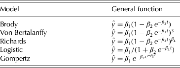
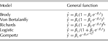
Five nonlinear models commonly used in the literature for describing animal growth curves were evaluated. In these models, shown in Table 2, y is the animal weight at time t i; β 1 the estimated body weight of the animal when t→∞ or asymptotic body weight; β 2 the constant of integration; β 3 the rate constant, which determines the spread of the curve along the time axis; and β 4 is the constant that determines the proportion of the final size at which the inflection point (IP) occurs. The IP can be determined using the equation 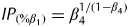 $IP_{(\% \beta _1 )} = \beta _4 ^{1/(1 - \beta _4 )} $, and the instantaneous absolute growth rate can be calculated using the equation
 $IAGR = \beta _3 \times Y_{{\rm est}} [(\beta _1 /Y_{{\rm est}} )^{1 - \beta _4} - 1]/(1 - \beta _4 )$, where Y est is the body weight estimated at a given time (Richards Reference Richards1959).
Evaluated growth curve functions
Nonlinear mixed model
A nonlinear mixed model methodology was used to obtain the growth curve parameters according to the following expression:
 $${\bf y}_i = f\,({\bf x}_{ij} {,}{\bi \beta}, {\bi u}_i ) + {\bi e}_i $$
where yi is a vector (n i×1) of recorded body weights for the subject i=1, 2,…, m; m is the number of goats; f is a nonlinear function of the covariate matrix xij; xij is a matrix (n i×2) of independent variables, in which the first column contains the ith age of measurement and the second column contains the jth subject (goat) whose body weight was measured; β is a vector (p i×1) of unknown fixed-effect parameters; u i is a vector (q i×1) of unknown random-effect parameters unique to the subject goat i and assumed to follow a multivariate distribution with a mean of zero and a conditional unstructured covariance matrix, n×n (G); and ei is a vector (n i×1) of the error term assumed to follow a multivariate random normal distribution with zero mean and conditional covariance matrix structure (R).
The dependent variable (y) in this case is influenced by quantitative (time) and qualitative (genotype) variables. The effects of the quantitative variables are analysed via nonlinear regression. However, it is also necessary to assess the effects of the qualitative variable on the dependent variable and the regression parameters; thus, dummy variables z 1 and z 2 were created, where for the +S genotype, z 1=0 and z 2=1, and for the +A genotype, z 1=1 and z 2=0. With this approach, it was possible to estimate growth curve parameters (β 1, β 2, β 3 and β 4) independently for each genotype.
The growth curve modelling consisted of two steps, as described below. First, a set of candidate nonlinear mixed models were formulated that were preliminarily analysed to choose the function with the best fit. This first step was used to evaluate which curve parameters should have a random effect component and compared them with the traditional fixed-effect model. However, despite the high hardiness with which nonlinear mixed model methodology treats the correlated errors, it is important to note that heterogeneity and correlated errors can occur even with the inclusion of random effects (Meng & Huang Reference Meng and Huang2010; Yang & Huang Reference Yang and Huang2011). Thus, a refinement of the model chosen in the first step was necessary to accommodate the violated model assumptions (second step).
First step
A central phase in the model-building of mixed-effects models is to decide which of the parameters in the nonlinear model require random effects to account for their between-subject variations and which can be treated as purely fixed effects (Pinheiro & Bates Reference Pinheiro and Bates2000). Thus, the random parameters u 1, u 2 and u 3 were created to account for between-subject variations for the β 1, β 2 and β 3 parameters, respectively, enabling curve parameters to be estimated for each goat (Littell et al. Reference Littell, Milliken, Stroup, Wolfinger and Schabenberger2006). No random parameter was created for the β 4 parameter in the Richards function because it was difficult to achieve the convergence criterion and the high correlations between the estimated parameters (overparameterized model). The following four combinations of random effects were evaluated: all of the parameters related to random effects (u 1, u 2 and u 3), only parameters related to β 1 and β 2 (u 1 and u 2), only parameters related to β 1 and β 3 (u 1 and u 3), and only that related to β 1 (u 1). To avoid problems with floating-point errors and overflows, β 3 was rescaled (×1000) in the models due to the difference in magnitude of this parameter in relation to the others.
First, the equations were fitted to each model and previously described combinations of random effects through PROC NLMIXED (SAS 9.3, see Appendix). The FIRO method was used to achieve convergence. The FIRO method uses the First-Order Method described by Beal & Sheiner (Reference Beal and Sheiner1982) to compute the integral over the random effects to the marginal maximum likelihood. The fixed-effects model was also estimated using PROC NLMIXED, except that, in this case, variance components were not included. The FIRO method does not support the model without random effects; thus, the Adaptive Gaussian Quadrature described by Pinheiro & Bates (Reference Pinheiro and Bates1995) was used. The estimated parameters, standard error and residual variance for the fixed-effects model were similar to those of the model obtained using PROC NLIN.
The following criteria were adopted to select the function that best described the growth curve of the goats: (1) convergence (the interactive process in NLMIXED converges at the nth interaction when  $(g_k H_k ^{ - 1} g_k )/(|l_k | + 1\,e^{ - 6} ) \lt 1\,e^{ - 8} )$(SAS Institute Inc. 2008)); (2) the final Hessian matrix is non-singular and positive definite; (3) the approach described by Burnham & Anderson (Reference Burnham and Anderson2002) and Vieira et al. (Reference Vieira, Campos, da Silva, Tedeschi and Tamy2012) using the Akaike information criterion (AIC), the difference among AIC values (Δr), the Akaike weights or likelihood probabilities (w r) and the evidence ratio or relative likelihood (ERr), which can be computed using the following equations:
 $${\rm AIC} = 2f\,({ \widehat\theta} ) + 2p$$
 $$\Delta _{\rm r} = {\rm AIC}_{\rm r} - \min {\rm AIC}_{\rm r} $$
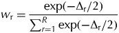 $$w_{\rm r} = \displaystyle{{\exp ( - \Delta _{\rm r} /2)} \over {\sum\nolimits_{r = 1}^R {\exp ( - \Delta _{\rm r} /2)}}} $$
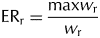 $${\rm ER}_{\rm r} = \displaystyle{{{\rm max} w_{\rm r}} \over {w_{\rm r}}} $$
where f() is the negative of the marginal log-likelihood function,  $\overset{ {\widehat \theta} $ is the vector of parameter estimate, and p is the number of parameters (SAS Institute Inc. 2008); and (4) a graphical analysis of the Pearson residuals against the predicted values was used to evaluate the model assumptions. The Pearson residuals were obtained for the fixed model and random model without a correlation structure as
 $r_i = e_i /\sqrt {\widehat{\sigma _e^2}} $ and for the model with a correlation structure (second step described below) as
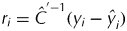 $r_i = \hat C^{' - 1} (y_i - \hat y_i )$, where
 $\hat C$ denotes the Cholesky root of the estimated R matrix (SAS Institute Inc. 2008).
Second step
The model with the best goodness-of-fit (combination between nonlinear equation and random parameters) was selected for further analysis.
Despite there being no sign of heteroscedasticity in the residuals of the chosen model, it was easy to identify high Pearson residuals obtained even when using random effects in the model. The higher values found for the Pearson residuals, many of them above three, were an indication of problems in the model. The first remedy would be to exclude the data from the data set and reparameterize the model, which would solve the problem but cause a loss of information.
Therefore, it was decided to use two tools to address this problem and the remaining correlated errors. The residual variance was modelled using the power-of-the-mean variance (PV) function. Using the notation described by Littell et al. (Reference Littell, Milliken, Stroup, Wolfinger and Schabenberger2006), the variance matrix R is assumed to be of the form  ${\bi R} = diag(\sigma ^2 |x_i ^' \beta ^ * |^\theta )$, where θ is the power to be estimated. In order to choose the value of θ, the power that minimized the approximate −2log-likelihood was calculated (Littell et al. Reference Littell, Milliken, Stroup, Wolfinger and Schabenberger2006); this θ value was estimated to be 2·91.
As previously noted, correlated errors can occur even when random effects are used in the model. These errors primarily occur if there are parameters in the function that do not have a random parameter to account for their between-subject variability. An error structure matrix can be modelled to account for this interrelation. When the model is fitted without modelling the serial correlation, the independently and identically distributed error structure is assumed to be Var[e i]=σ e2 and cov[e i,ej]=0. However, there is one intrinsic characteristic of the current data set that must be considered, namely, the unequally spaced measurement intervals for the animal subjects.
There is a range of structures available in the literature to address this issue. Structures that accept unequally spaced data have been described by Littell et al. (Reference Littell, Milliken, Stroup, Wolfinger and Schabenberger2006) and the SAS Institute Inc. (2008). Normally, the covariance is assumed to be a function of the distance between locations. If d ij denotes the distance between the measurements made on the same animal, the covariance models have the general form COV[e i,ej]=σe2[f(d ij)] (Littell et al. Reference Littell, Milliken, Stroup, Wolfinger and Schabenberger2006).
In the second step, all possible isotropic candidate structures described in the literature were examined; however, only two structures met the convergence criterion: the spatial power function (SP(POW)) and the MATERN function (SP(MATERN)).
The spatial power structure provides a direct generalization of the auto-regressive structure for equally spaced data and is assumed to be  $f\,(d_{ij} ) = \rho ^{d_{ij}} $. The MATERN isotropic covariance function is given as
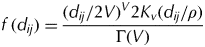 $f\,(d_{ij} ) = \displaystyle{{(d_{ij} /2V)^V 2K_v (d_{ij} /\rho )} \over {\Gamma (V)}}$ where K V is a modified Bessel function of the second kind of order V; Γ is the gamma function; ρ is a scalar parameter controlling the spatial range of correlation; and V is the ‘smoothness’ parameter, which allows greater flexibility for modelling the local spatial covariance. When V is small (V→0), the spatial process is assumed to be rough, and when V is large (V→∞), the process is assumed to be smooth (Littell et al. Reference Littell, Milliken, Stroup, Wolfinger and Schabenberger2006; Minasny & McBratney Reference Minasny and McBratney2007; SAS Institute Inc. 2008).
The NLMIXED procedure does not support the modelling of error structure directly; thus, the SAS macro %NLINMIX was used to refine the model to account for the chosen error structure. The restricted maximum likelihood was used along with the two expansion methods available in the SAS macro %NLINMIX (ZERO and EBLUP) to attempt to fit the model. The model adjusted in this way was compared with the fixed model and the random parameter model that was estimated using the previously described approach.
After selecting the model that best described the growth curves and included the previously estimated variance and covariance matrices, the hypotheses regarding one or more growth curve parameters could be tested. Thus, the difference between the growth curve parameters of the genotypes were tested, with the objective of simplifying the model (α=0·05).
Cross-validation
A cross-validation was performed to evaluate the goodness-of-fit of the chosen function. The original data set was randomly partitioned into two sub-data sets (training and test data), each containing 0·50 of the animals per genotype. The division of the original data set was conducted using PROC SURVEYSELECT from the SAS software (version 9.3). The first sub-data set (training data set) was used to fit the previously chosen best model (steps 1 and 2), and the second sub-data set (test data set) was used to evaluate the robustness of the model. Equation precision was measured with the coefficient of determination (R 2) between the observed and predicted values and the simultaneous F-test of the intercept and slope (intercept=0 and slope=1), whereas the accuracy of the equation was determined based on the concordance correlation coefficient (CCC) and the root-mean-square error prediction (RMSEP) and its decomposition into mean bias, systematic bias and random errors (Tedeschi Reference Tedeschi2006). The model evaluation was implemented using the Model Evaluation System v. 3.1.13 (http://nutritionmodels.tamu.edu/mes.html; verified 28 May 2013). Moreover, the parameters of the curve fit from the training data set were compared with the parameters of the curves fit from the original data set using 95% confidence intervals (IC95%).
Impact of the number of weights on random parameters
One of the major advantages of the nonlinear mixed model methodology is the possibility of having individual growth parameters adjusted for each animal and testing to determine how some parameters differ from the population mean. Using the chosen model and the individual deviation of asymptotic and constant rate parameters, it was possible to evaluate the effect of the number of weights on the parameters estimated for each goat using descriptive graphic analysis.
RESULTS
One function did not achieve the convergence criterion (Richards u 1, u 2 and u 3). The Richards (u 1 and u 2) model presented the singular Hessian matrix, which prevents its unique inversion. The Hessian matrix rendered by the Brody model was not positive definite, and the Gompertz (u 1, u 2 and u 3) model had at least one negative eigenvalue.
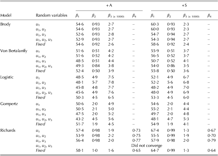
Table 3 shows the estimated parameters for all of the evaluated models and combinations of random variables. Although represented by the same Greek letters, except for asymptotic body weight (β 1), the estimated parameters cannot be compared among nonlinear functions (Forni et al. Reference Forni, Piles, Blasco, Varona, Oliveira, Lobo and Albuquerque2009). The only comparisons that are possible are between combinations of random variables or between assessed genotypes within each function. Among all of the scenarios that were assessed, the +S animals consistently had higher asymptotic body weights. Estimates of asymptotic body weight varied from 43·20 to 58·11 kg for the +A genotype and from 48·00 to 67·38 kg for the +S genotype.
Estimated parameters for the different models, random variable combinations and genotypes assessed

The calculated birth weight (calculated as time=0) for the Logistic and Gompertz (all combinations of random effects) models produced unrealistic estimated birth weight values. Reasonable estimates were made by the Brody and Richards (all combination of random effects) models.
High β 3 parameter values indicate higher precocity, i.e. a higher fractional rate at which the animal approaches asymptotic body weight (Brown et al. Reference Brown, Fitzhugh and Cartwright1976). The +A animals presented higher values (except for the Richards (u 1 and u 3)) for this parameter than the +S animals, possibly indicating earlier development.
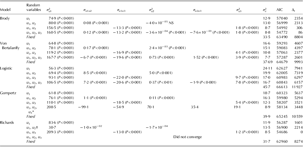
Table 4 shows the values of the criteria used to select the model that best describes goat growth in addition to the estimated variance and covariance components. The fixed-effect models were found to always display higher residual variance than the random-effect models did. The Richards (u 1 and u 3) function had the best fit. The value of Δr to the nearest model was 86, which, according to Burnham & Anderson (Reference Burnham and Anderson2002), indicates essentially no support. The large Δr values obtained became a calculation of the likelihood probability and evidence ratio unnecessary, as these criteria are equal to 1 for the Richards (u 1 and u 3) model.
Variance and covariance components, residual variances and information criteria of the fitted growth curves
* At least one eigenvalue was negative.
† Singular Hessian matrix.
NS: Not significant.
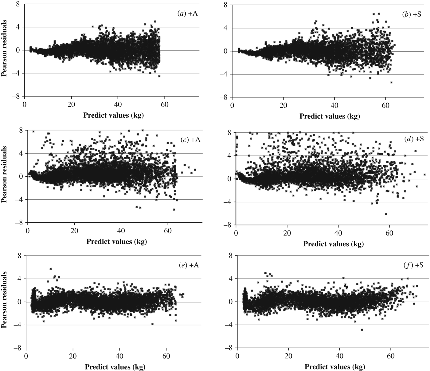
The random effects of the Richards (u 1 and u 3) model were significant (P<0·001). The value found for the component that measures the population variability of parameter β 1 was 209·3, and for β 3, this value was 1·20. However, high Pearson residuals were observed when the Richards (u 1 and u 3) model (Figs 1(b) and (c)) was used. Thus, this model was chosen for further analysis.
Pearson residuals of the Richards functions v. predicted values (kg) using the following approaches: (a, b) Fixed-effects model; (c, d) random-effects model (u 1 and u 3); (e, f) random (u 1 and u 3)+VP+SP(MATERN).
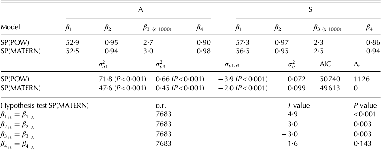
In the second step, the variance power and the modelled error structure matrix were included. Only the SP(POW) and SP(MATERN) structure achieved the convergence criterion. The use of these tools produced low values of the AIC when compared with the previous approach. The SP(MATERN) structure yielded better adjustments, as determined by the fact that Δr=1126 (Table 5).
Reparameterized Richard model parameters with error structure
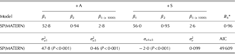
Using the SP(MATERN) error structure, there were differences between estimated parameters β 1 (P<0·001), β 2 (P=0·003) and β 3 (P=0·003) of the genotypes evaluated; however, there was no difference in the β 4 parameter (Table 5). Therefore, the model was reparameterized to account for just one β 4 parameter. The final parameters adjusted for each genotype were as follows: β 1=52·8 (s.e.=0·46), β 2=0·94 (s.e.=0·002) and β 3=2·83 (s.e.=0·066) for the +A animals, and β 1=56·0 (s.e.=0·59), β 2=0·95 (s.e.=0·002) and β 3=2·63 (s.e.=0·079) for the +S animals. The common β 4 parameter was 0·96 (s.e.=0·013). The variance components were σ2u1=47·5, σ2u3=0·46 and σu1u3=−2·0 (P<0·001) (Table 6). The growth curves are shown in Fig. 2.
Adjusted growth curve for the two genotypes evaluated.
Reparameterized Richard model with error structure and just one β4 parameter
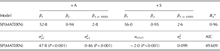
* Common β 4 parameter.
The IP was determined as a function of β 4 (Richards Reference Richards1959). This parameter did not differ between the evaluated genotypes; the IP at the same proportions of asymptotic body weight for both genotypes (0·36 of β 1) yielded 19·1 and 20·2 kg for genotypes +A and +S, respectively.
Figure 1 shows the Pearson residuals for the Richards model plotted against the predicted values (kg) by genotype for the Fixed model (Figs 1(a) and (b)), the Random model (u 1 and u 3) (Figs 1(c) and (d)) and the Random (u 1 and u 3)+VP+SP(MATERN) model (Figs 1(e) and (f)). When the function was fitted using the traditional approach, heteroscedasticity and the correlated errors occurred. In contrast, when random effects were added to the model, there was an improvement in the quality of the fitting; however, there were high Pearson residuals in this case, and correlated errors are easy to identify by the shape of the plotted residuals. This increase in residuals occurred once there were two common parameters (β 2 and β 4) in the functions, even when the errors were assumed to be independent. The variance power and error structure modelling yielded a better fit, and the Pearson residuals were within an acceptable range.
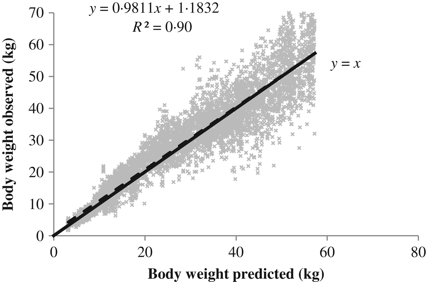
The Richards (u 1 and u 3)+VP+SP(MATERN) modelling approach was used to fit the training data set in the cross-validation analysis. The parameters fitted (data not shown) did not differ from the parameters fitted from the original data set, indicating that the chosen approach was effective even when using a reduced data set. When using the test data set to evaluate the model, the simultaneous F-test for the intercept (1·18±0·14) and slope (0·98±0·0045) rejected H0 (R 2=0·90). The CCC obtained was 0·95 (ranging from 0 to 1), indicating high accuracy. The RMSEP was 5·48 kg, and its decomposition indicated a high contribution from the random errors (98·37%), whereas the contributions of the mean bias (1·47%) and systematic bias (0·32%) were negligible. Figure 3 shows the relationship between the observed and predicted body weight values from the cross-validation.
Linear regression between observed and predicted body weights (dashed line). The continuous line is the Y=X line.
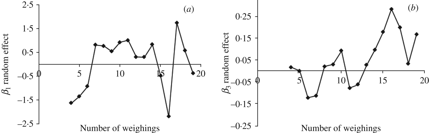
Fig. 4 shows that there was no apparent effect on the random parameter estimates from the number of weight measurements.
Effect of the number of weight measurements on the random effects for the (a) u 1 random parameter and (b) u 3 random parameter.
DISCUSSION
Growth curves and random effects
The nonlinear mixed model has as its main feature the partitioning of error variation into within- and between-subject variations. The fixed effects β 1, β 2, β 3 and β 4 represent the mean values of the parameters in the population of individuals. The individual deviations are represented by the random effects u 1, u 2 and u 3, which are assumed to be distributed normally with mean 0 and unstructured covariance matrix G.
For models with only the variance component linked to asymptotic body weight, the error variation was partitioned into variation within goats ( $\sigma _e^2 $) and the variation between goats (
 $\sigma _{u1}^2 $). When two variance components were added to the variation between goats, the error variation was partitioned into variation due to asymptotic body weight, the sigmoidal-shaped curve of each animal and the covariance between these terms ($\sigma _{u1}^2 $,
 $\sigma _{u2}^2 $ and $\sigma _{u1u2} $), or due to the asymptotic body weight, rate constant and covariance between these terms ($\sigma _{u1}^2 $,
 $\sigma _{u3}^2 $ and
 $\sigma _{u1u3} $), and so on, when three random effects were added; however, when three variance components were added in the growth curve model, there were indications of overparameterization and more highly correlated parameters, causing problems with convergence and the Hessian matrix.
In consequence, the estimate of the random effects (u 1, u 2 and u 3) of each goat represents the deviation of a determined parameter from its corresponding parameter for its population average. For example, the mean asymptotic body weight of the population of goats with +A genotype is 52·7 kg (Table 6), and the specific estimate of random effects for a specific goat is 5·9 kg (empirical best linear unbiased prediction – EBLUP). Therefore, the mean asymptotic body weight estimated for this specific animal is 58·6 kg, independent of short-term fluctuations in weight due to extraneous environmental effects such as climate and food supply as well as lactation and pregnancy. Thus, the mean estimated parameters are not greatly affected by these types of weight fluctuations. In fact, these parameters represent the mean value of the growth pattern of the goats on the production system.
It is possible that including biologically significant parameters with random variables in the model would reduce the residual variation, given that this tool reduces variability due to the parameters that have probability distributions and that can vary greatly from animal to animal, such as asymptotic body weight or rate constant. The random effect estimate measures the difference between the value assigned to each individual and the average population value (Aggrey Reference Aggrey2009).
The high values observed for $\sigma _{u1}^2 $ in most of the estimated models indicate the considerable contribution of this parameter in the residual variance component when this random variable is not added to the general model. Thus, it is important to incorporate this effect when using this methodology to estimate growth curves.
The $\sigma _{u3}^2 $ component was almost always found to be significant. In addition, adding the random effects linked to the rate constant improved the estimated model fit, a fact that was validated by better selection criteria (residual variance and AIC) when including this component. Moreover, the significance of this parameter indicates that the rate constant varies among the goat population and is thus subject to breeding programme selection.
A major advantage of selecting a nonlinear mixed model methodology to fit livestock growth curves is the possibility of including population variation measurements in stochastic models to predict animal performance. Normally, models predicting animal performance are deterministic, static and empirical, and for the same input, there is only one output that is modelled from the averages, with little or no emphasis on population variation (Pomar et al. Reference Pomar, Kyriazakis, Emmans and Knap2003). Therefore, when small samples are used, such as in the case of small farms, the errors become greater, especially when the model parameters vary greatly, as is the case for asymptotic body weight.
Understanding the variation among animals for the more widely variable parameters of the livestock system (dry matter intake, growth parameters, nutrient use efficiency, etc.) using stochastic components can be essential for understanding the mechanisms involved in population response to certain conditions (Pomar et al. Reference Pomar, Kyriazakis, Emmans and Knap2003). Linking these variations to dynamic models, for which the phenomena are understood over time, and to mechanistic models, for which the biological principles are understood and explained, can make the predictions of such models more credible.
The significant differences in the asymptotic body weight and constant rate parameters of the data are indicative of differences in the growth pattern between the genotypes. Alpine goats probably achieve their mature weight earlier than Saanen goats do, as indicated by the higher rate constant of growth and lower asymptotic body weight estimated for this genotype. This knowledge can be used by farmers to choose between genotypes depending on their interest. In addition, the different asymptotic body weights might be useful in mechanistic models, such as the Small Ruminant Nutrition Systems (SRNS) (Tedeschi et al. Reference Tedeschi, Cannas and Fox2010), which makes use of this parameter in its set of equations to predict the degree of maturity for goats. This information is already available for cattle and some sheep genotypes; however, the data set pertaining to goats needs to be expanded.
The Von Bertalanffy, Logistic and Gompertz models have a fixed IP relative to asymptotic body weight, which limits the biological interpretation of these functions due to the lack of flexibility in the estimation of the trend in the instantaneous absolute growth rate. In the case of the Richards model, the IP is variable and is a function of the β 4 parameter. The best model had common parameter β 4=0·9642 [IC95% 0·9394–0·9890], which yields a transitional function in form between the Brody (β 4=0) and the Gompertz (β 4=1) functions (Richards Reference Richards1959).
The flexibility of the β 4 parameter is the most important advantage of the Richards function. The IP in goats (0·36 of asymptotic body weight) may differ from the fixed IP adopted by the other functions. The IP occurs where the estimated instantaneous absolute growth rate changes from an increasing to a decreasing function. This information might be useful for strategic plans for goat feeding; information regarding the timing for the greatest capacity of the animal growth could be critical for plan optimization. Moreover, it is expected that from this point (c. 20 kg) onward, there is a decrease in growth rate, indicating a necessity for a change in feeding strategy.
Despite the fact that the genotypes have the same origin and are often considered similar in terms of productivity (only visibly different in their coats), differences have been found in their lactation curves (Guimarães et al. Reference Guimarães, Rodrigues, Sarmento and Rocha2006) and now, in the present study, in their growth patterns. This result indicates the need to use separate models (growth, lactation, etc.) for these two genotypes to predict animal response.
Modelling of the error structure
As noted by Littell et al. (Reference Littell, Milliken, Stroup, Wolfinger and Schabenberger2006), the first tool to be chosen when using the SAS software to fit a nonlinear mixed model is PROC NLMIXED, as it is more general because it accepts other distributions for the dependent variable; however, when it is necessary to model the error structure, the SAS macro %NLIMIX becomes more useful. Additional differences between the two approaches with relation to the estimation method can be found in Littell et al. (Reference Littell, Milliken, Stroup, Wolfinger and Schabenberger2006) and Vonesh (Reference Vonesh2012).
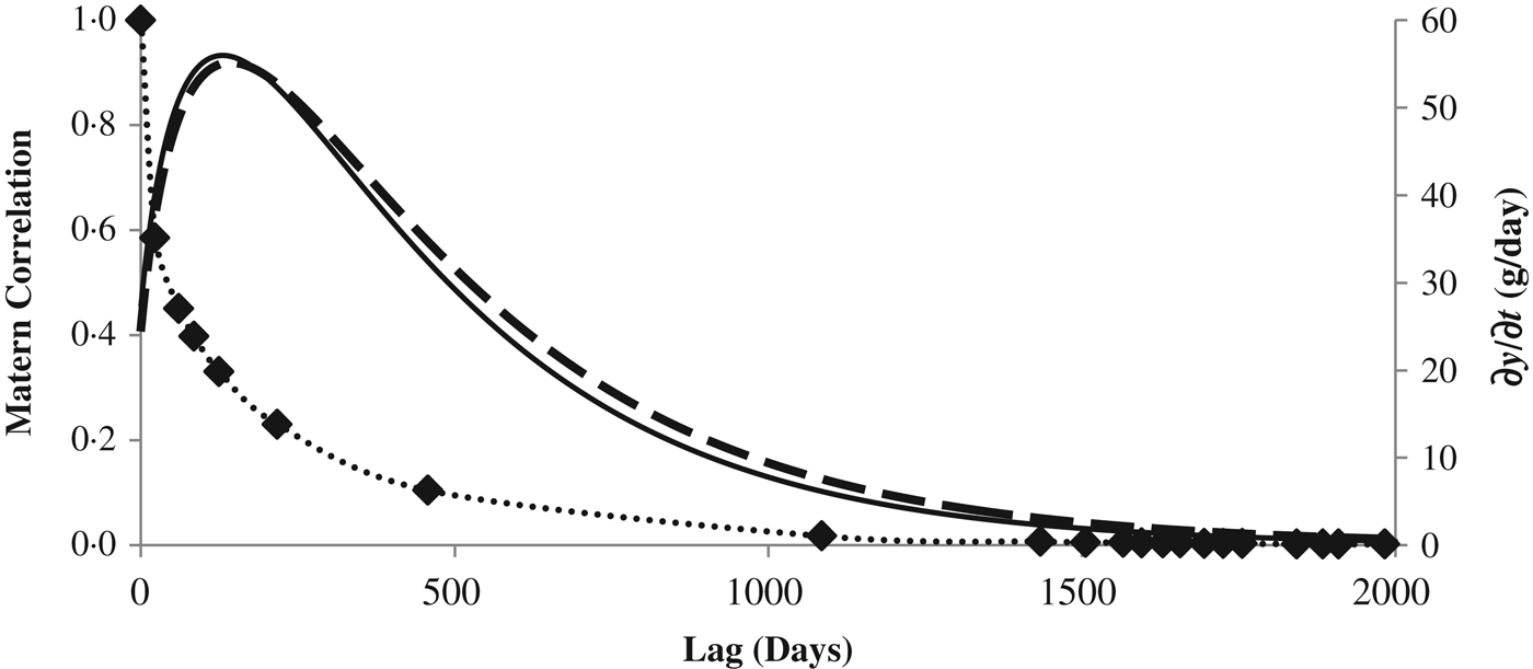
The SP(MATERN) structure has been historically used in spatial studies and has two parameters: ρ=411·02 (s.e.=52·27) and V=0·1471 (s.e.=0·006) (P<0·001). The lower value found for the V parameter implies that the correlation decreases abruptly between measurements. To illustrate this behaviour, the correlation was plotted between the measurements made on the animal with the maximum number of weight values (21 data points, with the first measure made at birth and the last at 1984 days old) (Fig. 5). The correlation decreases more rapidly over time, so that the correlation between two measurements with an interval of 23 days was 0·59. However, this finding is an indication that the correlation between two measurements was relatively well controlled.
The left axis shows the MATERN correlation function v. Lag (days) (point line). Black diamonds (◆) correspond to the values for animals with 21 weight measurements during their lifetime. The right axis shows the instantaneous absolute growth rate (g/day) for +S animals (continuous line) and +A animals (dashed line).
The possible reason that the SP(MATERN) structure adjusted better to this data set is the difference between the measurements found here. The current data included 1–1190 days of difference between two consecutive measurements (Lag). Obviously, two measurements taken at a close interval are typically more highly correlated than measurements taken at more distant time points (Littell et al. Reference Littell, Milliken, Stroup, Wolfinger and Schabenberger2006). In the current data set, 0·61 of the measurements were made before the animals were 1 year old, which means that the data are temporally close; the IP calculated in the Richards models occurs at 19·05 and 20·22 kg for the +A and +S genotypes, respectively, which occurs at c. 131 days old. Measurements taken close to these points will show a lower correlation than measurements taken far from them, because the higher instantaneous absolute growth rate observed around these inflection points. Figure 5 shows this relationship.
Cross-validation
Despite the fact that the simultaneous F-test for the intercept and slope rejected the null hypothesis, the high coefficient of determination indicates that the approach chosen is robust enough to estimate the body weight of goats. Furthermore, the RMSEP presented a relatively low value (5·48 kg) with a great contribution from random errors in the total error prediction. This finding indicates that effects that are not controlled are the main factors affecting the predictions. As shown in Fig. 3, the predictions are more credible in the early phases of growth, at lower body weights. Once there is a small variation around the average prediction, an increase in body weight leads to an occurrence of factors that are not controlled and operate to expand the variation around the estimated body weight; however, the average body weight estimated remains without bias, as indicated by the almost total overlap between the dashed line and the continuous lines.
Historically, the growth curve parameters for goats have not been evaluated using adequate statistical approaches, which may have created biases for the estimated values. The equations presented in the current paper are expected to yield more credible predictions for estimated mean values and population variations for some parameters.
Effects of number of weight values on the random effect estimates
Nonlinear mixed models are a strong tool for modelling and understanding population variability by incorporating random effects to account for between-subject variations. Apparently, the lack of influence of the numbers of weight measurements on random effects is another advantage of this method. Thus, this approach can be used to select animals that are different from the population average with regard to their rate of growth and those with asymptotic body weight.
CONCLUSION
The Richards model is adequate for describing the growth curve of dairy goats. The nonlinear mixed model methodology is an efficient tool to address growth curve features such as heteroscedasticity and correlated errors. Assigning biologically significant parameters with random effects is suggested, thus reducing the residual variance and making the estimates more credible. Moreover, evaluation of the modelling structure error is recommended to account for possible errors correlated even using random effects. Different Richard growth curve parameters should be used for the predominantly Alpine and Saanen genotypes because there are differences in their growth patterns.
J.G.L. Regadas Folho received a scholarship from the Capes Foundation – Process no.: 1528/12-2.
APPENDICES
SAS code:
Fixed model
PROC NLMIXED; /*Gaussian quadrature algorithm*/
/* Initial parameter estimates from PROC NLIN to start iterations;*/
parms b01=56 b11=59
b02=.9 b12=.97
b03=1.2 b13=1.5
b04=.7 b14=.8
s2e=20;
/*coding dummy variables for the goat genotypes*/
b1=b01*z1+b11*z2;
b2=b02*z1+b12*z2;
b3=b03*z1+b13*z2;
b4=b04*z1+b14*z2;
/*nonlinear Richards model*/
pred= b1*(1−b2*exp((−b3/1000)*x))**b4;
model y ~ normal (pred,s2e);
run;
Random model
PROC NLMIXED method=firo; /*FIRO algorithm*/
parms b01=52 b11=53
b02=.9 b12=.97
b03=1.9 b13=2
b04=.7 b14=.8
s2u1=30 c13=.99 s2u3=1.5 s2e=10;
b1=b01*z1+b11*z2+u1; /*variance components u1 and u3 added*/
b2=b02*z1+b12*z2;
b3=b03*z1+b13*z2+u3;
b4=b04*z1+b14*z2;
pred= b1*(1−b2*exp((−b3/1000)*x))**b4;
model y ~ normal (pred,s2e) ;
/*Specifying random parameters with normal distribution */
random u1 u3 ~ normal ([0,0],[s2u1,c13,s2u3]) subject=animal ;
run;
Random model+Variance Power+Error Structure Model
%nlinmix(data=cresc, /*Specifies the SAS data set*/
/*Coding dummy variables for the goat genotypes and request the nonlinear Richards model*/
model=%str(
b1=b01*z1+b11*z2+u1;
b2=b02*z1+b12*z2;
b3=b03*z1+b13*z2+u3;
predv= b1*(1-b2*exp((-b3/1000)*x))**b4;
),
/*Initial parameters estimated*/
parms=%str(b01=53 b11=57 b02=0.9 b12=0.97 b03=2.7 b13=2.2 b4=0.9),
/*Modelling the variance power statement*/
derivs=%str(
wt = 1/predv**(2.91*0.5);
),
/*Specifies the MIXED procedure to be executed for each iteration*/
stmts=%str(
class animal;
model pseudo_y = d_b01 d_b11 d_b02 d_b12 d_b03 d_b13 d_b4 / noint notest solution cl residual outp=pred_matern;
/*Specifies the random parameters and matrix G*/
random d_u1 d_u3 / subject = animal type = un solution;
/*Specifies the matrix R*/
repeated / subject=animal type=sp(matern)(x);
weight wt;
),
/*Request the expansion method*/
expand = zero,
/*Request the REML method and test the variance components parameters*/
procopt = %str(method = reml) covtest
)
run;