4.1.1 Route to stagnation and steady axisymmetric BVB

Figure 4(a) shows an axisymmetric steady swelling that develops centred about $x=5$ for a pre-breakdown swirl of $S=1.38$ . Billant et al. (Reference Billant, Chomaz and Huerre1998) have not reported the presence of a swelling and Leibovich (Reference Leibovich1978) noted, from early experiments, that swellings are most likely ephemeral features that disappear within a short time and considered them to be spurious artefacts in axisymmetric simulations. However, close to the threshold of VB, the occurrence of such swellings in the core region, as precursors to VB, has been observed in simulations using the Grabowski profile (Grabowski & Berger Reference Grabowski and Berger1976; Ruith et al. Reference Ruith, Chen, Meiburg and Maxworthy2003). It should be noted that the theory of Benjamin (Reference Benjamin1967) predicts the existence of such swellings, while Oberleithner et al. (Reference Oberleithner, Paschereit, Seele and Wygnanski2012) reported observing a local positive minimum in the time-averaged velocity along the jet axis for pre-breakdown swirls in the case of turbulent swirling jets, suggesting a swelling’s presence. In experiments on flows in cylinders with rotating end walls, Escudier (Reference Escudier1984) noted an ‘hour-glass structure’ that appears for swirls slightly lower than that at which VB occurs. Wang & Rusak (Reference Wang and Rusak1997) have noted, based on previous results, that a continuous transition to VB with increasing swirl, by means of a swelling, would likely occur only below a critical Reynolds number.

Figure 4.

Projected streamlines on meridional plane for (a) pre-breakdown swelling at $S=1.38$ and (b) steady BVB at $S=1.4$ .

For $S>S_{c}$ , the stagnation point moves upstream with increasing swirl, while a bubble is formed downstream (figure 4 b). The bubble observed here is commonly described as one celled, similar to those observed in experiments of Brücker & Althaus (Reference Brücker and Althaus1992) and simulations of Ruith et al. (Reference Ruith, Chen, Meiburg and Maxworthy2003), and is named so due to the presence of a single toroidal vortical structure. Billant et al. (Reference Billant, Chomaz and Huerre1998) have reported a single case which shows velocity fields for BVB (figure 7) with what is possibly a two-celled structure (Faler & Leibovich Reference Faler and Leibovich1978). It is noted that a sustained two-celled bubble occurred at higher swirls in hysteresis studies (§ 4.3), which will be reported elsewhere.

4.1.2 BVB with spiral tail

Starting from $S=1.49$ , the flow evolved towards an axisymmetric quasi-steady state containing a bubble but succumbed to helical instabilities leading to the eventual appearance of a spiral structure ( $m=+1$ ) in the bubble’s wake which rotates about the jet axis at a constant frequency. Thus, an increase in $S$ induces a transition from a steady flow to one which is periodically unsteady, indicating a supercritical Hopf bifurcation. The onset of breakdown at lower swirls than that above which the helical instability arises, has been noted for turbulent swirling jets by Oberleithner et al. (Reference Oberleithner, Paschereit, Seele and Wygnanski2012), who inferred the same trend to hold in the laminar regime based on the observations reported in Liang & Maxworthy (Reference Liang and Maxworthy2005). Additionally, a similar behaviour has been confirmed for the Grabowski profile in Meliga, Gallaire & Chomaz (Reference Meliga, Gallaire and Chomaz2012). However, Loiseleux & Chomaz (Reference Loiseleux and Chomaz2003) have noted the development of a single helical mode for pre-breakdown swirls in their studies on swirling jets.

Figure 5.

Meridional projections of (a) positions of tracers released from $r=0$ and $r=0.1$ at $t=100$ and (b) pathlines of tracers released from $r=0$ for the case of $S=1.5$ , outlining a bubble envelope unaffected by instability and the presence of a spiral tail downstream.

Features of this type of BVB are described using a typical case of $S=1.5$ . The long-time spatial structure for this case is visualized by means of tracer particles at a given instant as shown in figure 5(a). The figure clearly outlines the spiral structure of $m=+1$ embedded in the wake (approximately $x\geqslant 4$ ), while the bubble remains axisymmetric and unaffected by the spiral. These visualizations form the basis for referring to this type as BVB with a spiral tail (see also Sarpkaya Reference Sarpkaya1971, figure 5b). This is qualitatively different from most cases studied using Grabowski’s profile (Ruith et al. Reference Ruith, Chen, Meiburg and Maxworthy2003; Meliga et al. Reference Meliga, Gallaire and Chomaz2012), where instability growth was observed over the entire bubble region, with the bubble and the stagnation point at its nose affected, a characteristic of SVB. This suggests that the instability features for the two flows might be different. This was confirmed to be the case and will be discussed in § 5.

Projected pathlines based on tracer particles released from the inlet at $r=0$ are shown in figure 5(b). The abrupt expansion associated with VB ( $x\approx 1$ ) is vividly captured by this plot. It is evident that the tracers, after navigating over the bubble’s envelope in an axisymmetric fashion, reverse back to enter into it near its downstream end, following which they reside within the bubble for a considerable interval of time. Similar results have been observed in various experiments (e.g. Sarpkaya Reference Sarpkaya1971), where the dye injected at the inlet lingered within the bubble long after the injection was stopped. The streaks finally exited the bubble along a radially narrow region before spiralling outward into the wake, where they take helical paths towards the outflow boundary. The figure confirms that the flow remains axisymmetric in the bubble region. An approximate flow-through time for a particle to exit the domain was $150$ , highlighting the significant duration required to traverse the streamwise extent of $L_{x}=20$ . Winding of the particles into a helical structure is prominent at a distance of approximately $2$ from the downstream end of the bubble. While Billant et al. (Reference Billant, Chomaz and Huerre1998) do not report cases where the spiral is positioned as seen here, experiments in tube-vane arrangements (e.g. Sarpkaya Reference Sarpkaya1971; Faler & Leibovich Reference Faler and Leibovich1978) commonly reveal it to be positioned around one bubble diameter downstream, similar to the present case. Additionally, simulations based on such flow configurations (see Althaus & Weimer Reference Althaus, Weimer, Krause and Gersten1998, figure 11) show a similar structure.

Temporal characteristics of the flow were examined by placing probes at different streamwise positions. Three representative power spectral densities (PSD) of the fluctuating component $u_{y}^{\prime }$ at coordinates $(x,y,z)$ given by (1, 0, 0), (3, 0, 0.5) and (6, 0, 0.5) are plotted in figure 6(a). The fundamental frequency of $f_{0}=0.13$ was the same at all positions, with harmonics strengthening at downstream positions. Figure 6(b) shows contours of vorticity magnitude on a cross-sectional plane at $x=10$ at two instants $t=3.75$ apart, from which the rotation of the spiral vortex in the bubble’s wake can be inferred.

Figure 6.

(a) Power spectral densities of $u_{y}$ for the case of $S=1.5$ at different positions ( $x,y,z$ ): ——, (6, 0, 0.5); - - - -, (3, 0, 0.5); — ⋅ —, (1, 0, 0). The fundamental frequency is 0.13. (b) Contours of vorticity magnitude, $|\unicode[STIX]{x1D734}|$ , on plane $x=10$ showing the rotation of an $m=+1$ spiral structure’s cross-section at two instances, an interval of 3.75 apart. The inflow swirls clockwise.

4.1.3 Pulsating BVB

For the swirl range of $S\in [1.55,1.57]$ , a ‘pulsating’ type of BVB was observed. A representative swirl of $S=1.56$ studied using D40 (see table 1) is chosen for further scrutiny of this breakdown type. Past the initial transients and after the flow settled into a state similar to BVB with a spiral tail ( $m=+1$ ), the flow exhibited a peculiar behaviour with a pulsating temporal variation in the flow field. This is best illustrated by examining temporal variations in velocity components at fixed spatial positions in the domain. The time series of $u_{x}$ is shown in figure 7(a) at two locations on the flow axis including $x=1$ (vicinity of stagnation point) and 5 (wake) and additionally at $x=5$ , $y=0$ and $z=0.5$ . Figure 7 shows PSD of $u_{y}$ at the latter location. Variations of $u_{x}$ on the jet axis indicated a sinusoidal variation at one frequency, $f_{2}\approx 0.017$ , modulated by a periodic variation at a lower frequency, $f_{3}\approx 0.001$ . The former seems to be associated with pulsation events, while the latter was found to be related with the periodic intensification of such pulsation events. For comparison, at $S=1.5$ , $u_{x}$ remained constant with time at all locations on the axis, which can be anticipated assuming unsteadiness as originating only from a rotating $m=1$ helical mode. Except for $u_{x}$ on the jet axis and for locations in the upstream part of the bubble ( $x\leqslant 2$ ), all components at all positions, had temporal oscillations with frequencies $f_{2}$ , $f_{3}$ and additionally, $f_{1}\approx 0.093$ , the latter associated with the rotating helical mode, although there was a spread in the PSD about this frequency. The lowest frequency, $f_{3}$ , reduced with an increase in $S$ for the swirl range where pulsating BVB was observed.

Figure 7.

(a) Time series of $u_{x}$ for $S=1.56$ , at different locations ( $x,y,z$ ): - - - -, (1, 0, 0); —— (black), (5, 0, 0); —— (grey), (5, 0, 0.5). (b) Power spectral density of $u_{y}$ at (5, 0, 0.5).

Figure 8.

Streamlines at two different times for $S=1.56$ . A second set of closed streamlines (green) are observed only at the later instant, the intermittent appearance of which seems to cause the pulsating flow behaviour (see movie 2).

Dynamics of the flow is best understood by examining animations created using snapshots of velocity fields, available as movie 1 available athttps://doi.org/10.1017/jfm.2019.401 and instantaneous streamlines in movie 2. Figure 8 shows two representative instants showing streamlines. While a closed set of streamlines (red) associated with the bubble and observed for the case of $S=1.5$ is present at both $t=4000$ and 4100, a second set (green) representing a toroidal structure developed at the later instant. This intermittent formation of a ‘second cell’ was seen to influence the pulsating dynamics of the flow. While not studied here, it is noted that in hysteresis studies (see § 4.3), a two-celled BVB with a spiral tail was observed as the next new flow state at higher swirls. This state is characterized by a permanent second toroidal structure nested within that which is present for the one-celled case (figure 2 a). This suggests that the pulsating behaviour is a flow feature that is observed in the intermediate swirl range between two time-periodic flows – the one and two-celled BVB with spiral tail. It is noted that strong similarities exist between the present flow behaviour and that observed for the Grabowski profile by Pasche, Avellan & Gallaire (Reference Pasche, Avellan and Gallaire2018), including the presence of axisymmetric oscillations and multiple frequencies. However, no additional distinct helical structures which rotate at a different frequency could be identified using a temporal Fourier decomposition of time series of the velocity field, $\boldsymbol{u}(\boldsymbol{x},t)$ . An examination using tracer particles did not provide insights into these structural changes, although it was observed that after traversing the bubble envelope, due to non-axisymmetric unsteady flow in the downstream end of the bubble, some particles were engulfed into it, while others were convected along the spiral tail in the bubble’s wake (Pradeep Reference Pradeep2019). This is in agreement with observations made in experiments of Faler & Leibovich (Reference Faler and Leibovich1978), who noted a ‘simultaneous emptying and filling’ of a bubble in this downstream region.

It is not clear whether this type of BVB has been previously observed, although low frequency modulations have been reported for various swirling flows where VB was observed (Stevens, Lopez & Cantwell Reference Stevens, Lopez and Cantwell1999; Blackburn & Lopez Reference Blackburn and Lopez2000; Ruith et al. Reference Ruith, Chen, Meiburg and Maxworthy2003; Pasche et al. Reference Pasche, Avellan and Gallaire2018). In all cases, there are certain differences from the features observed here, as elaborated in Pradeep (Reference Pradeep2019).

4.2.1 Instantaneous features for $S=1.6$

Typical instantaneous features of CVB for a swirl of $S=1.6$ are as in figure 9, showing contours of axial velocity and vorticity magnitude on the meridional plane. The swirling jet entering the domain axially decelerated and a stagnation point developed close to the inlet at $x\approx 1$ , followed downstream by a sharp conical expansion as a thin sheet with an opening angle of ${\approx}90^{\circ }$ . This sheet enclosed a relatively large recirculation region of nearly stagnant flow compared to BVB. The weak reverse flow in this region had a minimum of $u_{x}$ around $-0.06$ . The flow took a paraboloid shape in the vicinity of the stagnation point, in agreement with observations in Billant et al. (Reference Billant, Chomaz and Huerre1998). The maximum of axial velocity for $x>5$ was ${\approx}0.2$ implying that there was reduced axial convection leading to long residence times in the downstream part of the domain. Similar to experiments, the conical sheet undulated beyond a distance of a few jet diameters downstream of the stagnation point, as seen in figure 9(b). The azimuthal component of velocity drastically reduced on the cone, and the flow downstream of the stagnation point was only weakly swirling.

Figure 10.

Axial velocity contours on different cross-sectional planes at $t=7500$ for $S=1.6$ . The figures indicate that the flow is axisymmetric upstream ( $x\leqslant 5$ ), but distorted downstream.

Cross-sectional features of CVB are shown in figure 10 by means of axial velocity contours at various streamwise positions. The conical sheet remained approximately axisymmetric for $x=5$ , while non-axisymmetric features became prominent at $x=20$ , where the flow along this sheet is almost parallel to the jet axis. By $x=30$ , the sheet configuration was severely weakened and distorted, with unsteady disorderly flow features observed. In experiments, the downstream flow attained a weakly turbulent state. Note that the recirculation zone in the core region is absent at $x=30$ .

Temporal features are best understood by examining videos of contours on meridional and cross-sectional planes provided as movies 3 and 4. The entire conical structure was found to rotate at a low frequency, similar to experiments where this motion was reported as being a major deterrent in scrutinizing the structure of CVB. In the vicinity of breakdown, the flow remained mostly steady with weak temporal variations in the opening angles, while downstream ( $x\geqslant 10$ ), rotation of the structure was observed. Flow structures were observed to be mostly restricted to a region of radius 25 for the entire duration of the simulation. Thus, it seems reasonable to assume that CVB is not directly influenced by the lateral boundaries placed at a radius of 40.

Figure 11.

Meridional projection of streaklines for $S=1.6$ at different times $t$ from the start of release ( $t=150$ , 400 and 650), showing disorganized features at downstream regions of cone and the recirculation zone. Only part of the domain is shown for clarity.

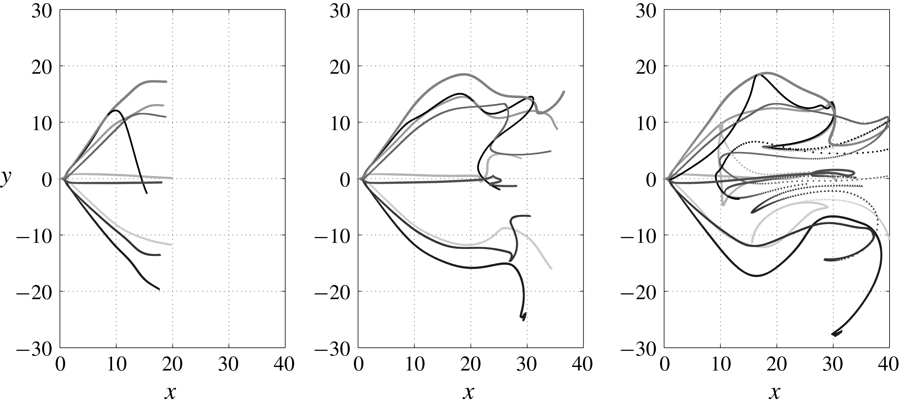
Visualizations based on tracer particles released, with initial positions at $r_{0}=0$ and $r_{0}=0.1$ (see § 2 for details), are shown at different instances in figure 11. A conical state was established by a simulation time of ${\approx}3000$ and particles were released starting $7800$ . The particles initially spread along an approximately axisymmetric conically expanding sheet, downstream of a stagnation point in the flow. At $x\approx 15$ , the radial expansion rate reduced and eventually led to the particles turning almost parallel to the jet axis. The relatively unsteady and non-axisymmetric nature of the downstream regions of flow can be inferred from inspecting streaklines for $t\geqslant 400$ with visualizations showing that while some curve radially inwards, others move outwards, with some entrained into the weak recirculation zone. It is evident from these visualizations that while the flow remains organized in the upstream region containing the conical sheet, its structure is distorted elsewhere, especially within the recirculation zone. Further, although the shortest duration in which a particle reached the outflow boundary was around $500$ , the average duration was extended considerably due to particles getting trapped into the recirculation zone, with residence times greater than 1000.

Computational difficulties abound in studying CVB due to the large radial spreading of the cone and slow unsteady non-axisymmetric motions in the downstream regions. The former requires a large domain to simulate the entire structure in addition to sufficient grid resolution and appropriate numerical scheme to resolve the thin sheet. The latter deters local grid refinement and increases the required simulation time to capture the evolution of the cone. With the focus on qualitative behaviour, the time-averaged flow features are reported next.

4.2.2 Time-averaged spatial structure for $S=1.6$

The velocity field was time averaged for a duration of approximately $2500$ starting from the time CVB was established. Additionally, assuming axisymmetry, the flow was azimuthally averaged for further statistical convergence. Figure 12(a) shows projected streamlines on the meridional plane. A large recirculation region encompassed by the cone with an approximate maximum radius of around 15 and an axial length of 25 can be seen. It is evident that the conical sheet eventually converges radially towards the core region, forming what can be crudely described as an enlarged ‘bubble’ containing a weak toroidal recirculation region. Counter-rotating vortices that represent this toroid intersecting the meridional plane have been observed in experiments of CVB (Billant et al. Reference Billant, Chomaz and Huerre1998). Figure 12(b) shows contours of the root-mean-squared fluctuating axial velocity component (other components not shown for conciseness). Variations of the opening angle of the cone can be inferred from this figure, while the flow in the vicinity of the stagnation point remained steady. It was observed that the maximum magnitudes of all components were only approximately $6\,\%$ of the velocity scale, indicating weak motions. The streamlines for $x\geqslant 30$ indicate an almost columnar flow. Weak axial vorticity was present here, implying that a weakened ‘vortex core’ exists downstream of VB. It is interesting to note that analogous structures qualitatively similar to those observed for BVB are present in CVB.

Figure 12.

Time-averaged features of CVB at $S=1.6$ shown on meridional plane: (a) mean projected streamlines and (b) contours of root mean square of fluctuating axial velocity.

Figure 13.

Streamwise variations along mean projected streamlines in solutions obtained at $S=1.6$ of (a) radial position, (b) slope of streamline, (c) projected velocity, (d) azimuthal velocity (lines) and circulation (symbols), (e) azimuthal vorticity and (f) pressure drop (lines) and Bernoulli head (symbols) for streamlines starting from $x=0$ : —— and ○, $r=0.5$ ; - - - - and $\times$ , $r=0.75$ ; — ⋅ — and ♢, $r=1$ . Insets show variations in the vicinity of the stagnation point ( $x\in [0,2]$ ). It can be inferred from these plots that CVB consists of a conically expanding thin sheet along which sharp reductions occur in velocity and pressure drop.

Variations of different flow properties along projected streamlines based on the azimuthally averaged mean flow are shown in figure 13. Figure 13(a) shows the radial positions of streamlines, $\unicode[STIX]{x1D70E}(x)$ , which begin from radial positions $\unicode[STIX]{x1D70E}(x=0)=0.5$ , 0.75 and 1 at the inflow plane. The streamlines achieved a constant slope of $\text{d}\unicode[STIX]{x1D70E}/\text{d}x\approx 1$ in the conical part of the sheet for $x<10$ (figure 13 b). The streamlines had an approximately constant curvature as the flow turned radially inward for $x\in [10,20]$ . It is interesting that an inward radial velocity develops, a feature shared with BVB. The velocity component along the projected streamlines dropped considerably in magnitude with $x$ , as seen in figure 13(c). The swirling component of velocity (figure 13 d) nearly vanished within a few diameters downstream of the stagnation point implying that the conical sheet is a weakly swirling structure. The symbols, representing circulation parameter $\unicode[STIX]{x1D6E4}=\unicode[STIX]{x1D70E}u_{\unicode[STIX]{x1D703}}$ , show that although the streamlines radially expand with $x$ , it too reduces. The azimuthal vorticity, $\unicode[STIX]{x1D6FA}_{\unicode[STIX]{x1D703}}$ , (figure 13 e) increased in magnitude past the stagnation point due to vortex tilting, but further downstream, dropped drastically in relation to the loss of gradients associated with the reduction in velocities. It is interesting to note the strong presence of both positive and negative $\unicode[STIX]{x1D6FA}_{\unicode[STIX]{x1D703}}$ close to the stagnation point associated with the inner and outer shear layers that demarcate the conical sheet. The pressure (figure 13 f) increased to values close to the ambient pressure $p_{\infty }$ of the chamber by $x=1$ (see inset) and remained so along the sheet. This confirms the assumption of Billant et al. (Reference Billant, Chomaz and Huerre1998) used as part of their breakdown criterion, that pressure at the stagnation point for CVB is given by $p_{0}=p_{\infty }$ . The Bernoulli head, $H=p+\boldsymbol{u}\boldsymbol{\cdot }\boldsymbol{u}/2$ , drops to negligible values by $x\approx 10$ . Thus, both $\unicode[STIX]{x1D6E4}$ and $H$ , which are preserved on streamsurfaces of axisymmetric inviscid flows, are strongly reduced by viscous actions. While the low $Re$ chosen for the present study can lead to strong viscous effects, CVB seems to amplify the role of viscosity by the formation of the thin conical sheet of flow. However, it must be noted that on the jet axis ( $r=0$ ), $H$ remained approximately a constant, confirming another assumption of the criterion of Billant et al. (Reference Billant, Chomaz and Huerre1998).

As $S$ was increased further to 1.8, the conical form was sustained, although the opening angle increased (not shown), with a larger recirculation region present. However, it remained unclear if the domain dimensions were adequate, and thus, details are not presented here, but can be found in Pradeep (Reference Pradeep2019).

4.2.3 Wide-open CVB

Mourtazin & Cohen (Reference Mourtazin and Cohen2007) reported observing what they referred to as a ‘wide-open’ cone (see figure 7 c) at high $Re$ , where the thin sheet opened out radially within a short distance downstream of the stagnation point, at an angle perpendicular to the jet axis. Similar observations have been noted in older experimental studies of swirling jets (Gore & Ranz Reference Gore and Ranz1964). This phenomenon was also observed in the present study for $S=2$ in D80. However, structures of $m=4$ were present and VB was in close proximity to the inflow plane and thus only a brief description of this state is provided and caution must be exercised when interpreting these results. Projected streamlines on $y=0$ plane at an arbitrary instant are plotted in figure 14(a). A stagnation point was present at $x\approx 0.8$ , downstream of which the flow was confined into a thin radially expanding sheet. Unlike the CVB observed at $S=1.6$ , (see figures 12 and 13 b), the streamlines here were found to have a positive curvature that led to the structure being wide open. This seems to be the major distinguishing feature of this type of CVB, with the flow almost reversing towards the inflow plane. While the flow was axisymmetric at upstream positions, a spurious $|m|=4$ structure developed, as seen from axial velocity contours on cross-sectional plane in figure 14(b). In spite of the presence of this structure, the breakdown feature of sharp radial expansion seen in experiments was still captured in the simulations. In simulations at higher $Re$ , the same type was observed, but with the flow being turbulent and without the $|m|=4$ structures; a detailed analysis of this type of CVB will be reported elsewhere.

Figure 14.

(a) Projected streamlines on positive $z=0$ plane based on instantaneous velocity fields for $S=2$ . (b) Axial velocity contours on different cross-sectional planes for the same. This type is identified as a ‘wide-open’ CVB, with the thin sheet turning perpendicular to the jet axis ( $x=5$ , $y=10$ ). Cross-section showed presence of possibly spurious $|m|=4$ modes.