





Introduction
Freshwater ecosystems represent about 1 % of the Earth’s surface and host 10 % of all the recorded species worldwide (Darwall et al. Reference Darwall, Smith, Allen, Holland, Harrison and Brooks2011; Strayer and Dudgeon Reference Strayer and Dudgeon2010b). They are hotspots for human activities, as they provide vital resources for people and a great array of services, amongst which water regulation, disturbance regulation, water supply and waste treatment are the most important (Strayer and Dudgeon Reference Strayer and Dudgeon2010). The ecosystem services provided by freshwater are estimated to be about USD 4 trillion worth per year, which is more than 20 % of all the ecosystems combined (Costanza et al. Reference Costanza, De Groot, Sutton, Van Der Ploeg, Anderson, Kubiszewski, Farber and Turner2014; Darwall et al. Reference Darwall, Bremerich, De Wever, Dell, Freyhof, Gessner, Grossart, Harrison, Irvine, Jähnig, Jeschke, Lee, Lu, Lewandowska, Monaghan, Nejstgaard, Patricio, Schmidt-Kloiber, Stuart, Thieme, Tockner, Turak and Weyl2018), making freshwater the most important resource human beings depend on to survive. In addition to humans, an important range of plants, animals and microorganisms depend on freshwater ecosystems for their survival. They provide suitable habitats for at least 126,000 plant and animal species (Balian et al. Reference Balian, Segers, Lévèque and Martens2008). But this number is probably an underestimate, as a lot of freshwater species are still to be described (Revenga et al. Reference Revenga, Campbell, Abell, De Villiers and Bryer2005).
Over the last decades, the rapid growth of the human population has led to the deterioration of the nature to fill the high demand in food production, socio-economic development and living space to meet current demand (Crist et al. Reference Crist, Mora and Engelman2017). This has resulted in an intensified impact on the environment. It has been shown that freshwater systems are among the most threatened of all the environments worldwide (Hannah et al. Reference Hannah, Brown and Milner2007; Revenga et al. Reference Revenga, Campbell, Abell, De Villiers and Bryer2005). Freshwater species are seriously declining around the world. A decline of about 83 % of the global freshwater biodiversity has been noted since 1970 (WWF 2018), and many tropical and sub-tropical wetlands, particularly swamp forests, have been lost or degraded since the 1950s (Revenga et al. Reference Revenga, Campbell, Abell, De Villiers and Bryer2005). Estimates suggest that at least 10,000–20,000 freshwater species are extinct or at risk (Sayer et al. Reference Sayer, Fernando, Jimenez, Macfarlane N.B., Rapacciuolo, Böhm, Brooks, Contreras-MacBeath, Cox, Harrison, Hoffmann, Jenkins, Smith, Vié, Abbott, Allen, Allen, Barrios, Boudot, Carrizo, Charvet, Clausnitzer, Congiu, Crandall, Cumberlidge, Cuttelod, Dalton, Daniels, De Grave, De Knijf, Dijkstra K.-D., Dow, Jörg, García, Gessner, Getahun, Gibson, Gollock, Grant, Groom A.E., Hammer, Hammerson, Hilton-Taylor, Hodgkinson, Holland, Jabado, Juffe Bignoli, Kalkman, Karimov and Kipping2025; Strayer and Dudgeon Reference Strayer and Dudgeon2010). This catastrophic decline of freshwater biodiversity is caused by the combination of different threats, notably habitat degradation, water pollution, over-exploitation, flow modification and species invasion, which are the five major categories (Dudgeon et al. Reference Dudgeon, Arthington, Gessner, Kawabata, Knowler, Levêque, Naiman, Prieur-Richard, Soto, Stiassny and Sullivan2006; Revenga et al. Reference Revenga, Campbell, Abell, De Villiers and Bryer2005; WWF 2018). Reid et al. (Reference Reid, Carlson, Creed, Eliason, Gell, Johnson, Kidd, Maccormack, Olden, Ormerod, Smol, Taylor, Tockner, Vermaire, Dudgeon and Cooke2019) have recently identified 12 emerging threats that appeared or were exacerbated during the decade 2010–2020 including changing climates, infectious diseases, expanding hydropower and cumulative stressors, which are suggested to be the most severe ones. All these pressures on freshwater ecosystems not only negatively affect the diversity of animal and plant species but also the water quality and quantity, the connectivity to other parts of the system and landscape and also habitat conditions (Ahmed et al. Reference Ahmed, Kumar, Kabir, Zuhara, Mehjabin, Tasannum, Hoang, Kabir and Mofijur2022; WWF 2018).
To effectively conserve freshwater habitats, it becomes urgent to evaluate their actual status in order to put in place appropriate management plans, which will be applied to important biodiversity areas as a priority. These plans rely on effective knowledge of the biodiversity of the different habitats (Dudgeon et al. Reference Dudgeon, Arthington, Gessner, Kawabata, Knowler, Levêque, Naiman, Prieur-Richard, Soto, Stiassny and Sullivan2006). Unfortunately, knowledge of the total diversity of freshwaters is very limited, particularly among invertebrates, and especially in the tropical zone that supports most of the world’s biodiversity (Ahmed et al. Reference Ahmed, Kumar, Kabir, Zuhara, Mehjabin, Tasannum, Hoang, Kabir and Mofijur2022; Dudgeon et al. Reference Dudgeon, Arthington, Gessner, Kawabata, Knowler, Levêque, Naiman, Prieur-Richard, Soto, Stiassny and Sullivan2006). Due to the urgency of conservation actions, rather than putting in place monitoring surveys, which are expensive and time consuming, it is preferable to rely on taxa that have been shown to be reliable surrogates of the diversity and habitat conditions (Heino et al. Reference Heino, Paavola, Virtanen and Muotka2005; Stewart et al. Reference Stewart, Underwood, Rachel and Walters2018). Monitoring freshwater quality in the tropics is difficult to put in place because of the high diversity found there. In such situations, dragonflies can serve as efficient indicators (Suhling et al. Reference Suhling, Sahlén, Gorb, Kalkman, Dijkstra, Van Tol, Thorp and Rogers2015). In fact, in their study on the effectiveness of surrogate species and their representativeness of freshwater species on the African continent, Darwall et al. (Reference Darwall, Holland, Smith, Allen, Brooks, Katarya, Pollock, Shi, Clausnitzer, Cumberlidge, Cuttelod, Dijkstra, Diop, Garcia, Seddon, Skelton, Snoeks, Tweddle and Vié2011a) found that dragonflies are effective surrogates for the diversity of other freshwater species (birds, mammals and amphibians). Furthermore, they make useful surrogates in the selection and prioritization of sites for aquatic conservation (Simaika and Samways Reference Simaika and Samways2009).
Odonata are actually used to evaluate the health status of freshwater ecosystems through many biotic indexes (Chovanec et al. Reference Chovanec, Schindler, Waringer and Wimmer2015; Golfieri et al. Reference Golfieri, Hardersen, Maiolini and Surian2016; Korbaa et al. Reference Korbaa, Ferreras-Romero, Ruiz-Garcia and Boumaiza2018; Simaika and Samways Reference Simaika and Samways2009, Reference Simaika and Samways2012; Vorster et al. Reference Vorster, Samways, Simaika, Kipping, Clausnitzer, Suhling and Dijkstra2020). They occur in almost all freshwater habitats, and many are restricted to some specific habitats such as forest streams and tree holes (Suhling et al. Reference Suhling, Sahlén, Gorb, Kalkman, Dijkstra, Van Tol, Thorp and Rogers2015). The ease of identification in the field, their well-known taxonomy and the habitat requirements known for many species make them established biological indicators of freshwater conditions in Africa (Samways and Simaika Reference Samways and Simaika2016; Simaika and Samways Reference Simaika and Samways2011). However, the level of information on Odonata in all the countries in Africa is not the same, with central African countries being amongst the least investigated on the continent (Dijkstra et al. Reference Dijkstra, Boudot, Clausnitzer, Kipping, Kisakye, Ogbogu, Samraoui, Samways, Schütte, Simaika, Suhling, Tchibozo, Darwall, Smith, Allen, Holland, Harrison and Brooks2011).
At the local scale, it is shown that habitat type and habitat structure are amongst the most important factors influencing the species richness and the composition of odonates’ communities. Odonata assemblages are associated with specific combinations of waterbody type, size, canopy cover, flow, depth, substrate, land-use systems and riparian vegetation (Ribeiro et al. Reference Ribeiro, Juen and Schlemmer Brasil2022; Dijkstra and Lempert Reference Dijkstra and Lempert2003; Hart et al. Reference Hart, Bowker, Tarboton and Downs2014; Oliveira-Junior and Juen Reference Oliveira-Junior and Juen2019; Seidu et al. Reference Seidu, Danquah, Nsor, Amaning and Lancaster2017, Reference Seidu, Nsor, Danquah and Lancaster2018). Increased habitat heterogeneity can lead to higher Odonata diversity, while disturbances, by converting shaded forest streams into open and reducing environmental integrity, shift assemblages dominated by habitat-specialist Zygoptera to those dominated by widespread generalist Anisoptera (Hart et al. Reference Hart, Bowker, Tarboton and Downs2014; Oliveira-Junior et al. Reference Oliveira-Junior, Shimano, Gardner, Hughes, de Marco Júnior and Juen2015). Studies also show that conditions surrounding water bodies can drive communities’ composition of odonates (Ribeiro et al. Reference Ribeiro, Juen and Schlemmer Brasil2022; Oliveira-Junior and Juen Reference Oliveira-Junior and Juen2019; Seidu et al. Reference Seidu, Nsor, Danquah, Tehoda and Oppong2019). While those kinds of studies are common in Amazonian systems, they are still very scarce on the African continent, especially in Central Africa, which limits the use of Odonata habitat-based assessments in this region.
The present work aims at evaluating the influence of habitat types on the community composition of Odonata. Adults were sampled in five water bodies representing different types of habitats in the South Region of Cameroon. We hypothesized that (a) the species’ richness, abundance and community composition of species will vary significantly between the different habitats, (b) some species will show a strong preference for a specific habitat. These predictions are supported by previous literature. In fact, some odonate species with narrow ecological requirements are expected to be strongly associated with particular habitat types or environmental-integrity levels. For example, studies have identified odonate species associated with degraded streams, urbanized habitats, different levels of habitat integrity, lentic or lotic habitats, showing that indicator species can provide information on environmental quality (Oliveira-Junior et al. Reference Oliveira-Junior, Shimano, Gardner, Hughes, de Marco Júnior and Juen2015; Monteiro-Júnior et al. Reference Monteiro-Júnior, Juen and Hamada2014, Seidu et al. Reference Seidu, Danquah, Nsor, Amaning and Lancaster2017, Seidu et al. Reference Seidu, Nsor, Danquah, Tehoda and Oppong2019).
Materials and methods
Study sites
The study was carried out in the locality of Minko’o (sub-division of Meyomessala, Division of Dja & Lobo, South Region, Cameroon). Minko’o is situated 7 km from the western outskirt of the Dja Biosphere reserve and 18 km far from the town of Meyomessala (Figure 1). The locality is influenced by an equatorial climate with 4 seasons and is dominated by evergreen forest (Letouzey Reference Letouzey1986). The average temperature in the area is 23.5°C (13°C–36°C); and the average relative humidity is 86.50% (20–100%).
Location of the study habitats A: forest swamp, B: bamboo stream, C: forest stream, D: open stream, E: swampy canal.

Five habitats were selected for sampling in the locality. The selection of the sites was based on the habitat type, their accessibility and the consent by the landowners (Figures 1 and 2).
Pictures of the study habitats: A: forest swamp, B: bamboo stream, C: forest stream, D: open stream, E: swampy canal.

The forest swamp (N3°05’54.9’’, E12°21’45.6’’) is a network of four connected puddles in a swampy forest, high canopy cover. Araceae is the dominant vegetation around; mud and dead leaves form the substrate of the puddles. Anthropogenic activities on this site were limited to the presence of a nearby trail used by villagers to go to the farm. The bamboo stream (N3°05’55.8’’, E12°21’45.1’’) is a large stream near the road with a very low water flow, surrounded and covered by China bamboo (Bambusa vulgaris Schrad. ex J.C. Wendl., 1808); some small patches of Araceae were also found on the stream bed. Gravels and dead leaves of bamboo constitute the bottom. Populations would generally cut mature bamboo for craft and construction. The forest stream (N3°05’54.7’’, E12°21’21.2’’) is a stream (about 2 m wide) surrounded by swamp and have some tall trees on the bank. The canopy is closed, and the undercover is made principally of Maranthaceae. The water flow is slow, and the substrate is sandy with some dead branches and leaves. Villagers mostly use this stream to collect Maranthaceae leaves that are used for cooking.
The open stream (N3°06’02.0’’, E12°21’10.0’’) is a stream with no canopy cover, had a low water flow and had blackish water. The substrate was gravelly. Anthropogenic activities around included laundry, washing up the dishes and motorbikes, fishing and bathing. The bankside vegetation (weeds and some palm trees) was sometimes cleared by villagers when it became important. The swampy canal (N3°06’02.8’’, E12°21’09.5’’) is a manmade canal (about 10 m long and 0.5 m large) put in place to evacuate the excess water from a well (1.5 x 1.5 m). The excess of water flows in a very muddy canal (of) with a lot of detritus; the said canal ends in a swamp. This canal is very muddy with a lot of detritus. It is situated in a secondary forest with some big trees, and the canopy is moderately opened. The place is very well managed (frequently cleaned), as local people collect the water from the well for drinking and domestic use.
Sampling procedure
Odonata sampling was carried out in November 2015, February 2016, June 2016 and then monthly from August 2016 through June 2017; for a total of 14 visits in forest swamp, forest stream and open stream. The bamboo stream and the swampy canal were visited 13 times, as they were visited simultaneously with the other three sites, except in November 2015. Sampling at each site was carried out from 8 a.m. to 6 p.m.
The adults were captured using a hand net with a telescopic handle. Some species, such as big Aeshnidae and some Libellulidae, were recorded only by sight, as they are fast-flying and very agile, and hence make it difficult to catch them with the net.
Specimens were mostly identified in the field, but when it was impossible to do so, the first captured individuals of each unidentifiable morphospecies were kept in a properly labelled triangle envelope for further identification in the laboratory.
Identification of specimens
Specimens were identified under a stereomicroscope using the handbook from Dijkstra and Clausnitzer (Reference Dijkstra and Clausnitzer2014), the African Dragonflies and Damselflies Online (Dijkstra Reference Dijkstra2017) and the help of Dr K.-D. B. Dijkstra.
Data analysis
Diversity of Odonata
Eight non-parametric species richness estimators were used to evaluate the success of capture of Odonata (ACE: abundance-based coverage estimator, ICE: incidence-based coverage estimator, Chao 1: Chao’s abundance-based richness estimator, Chao 2: Chao’s incidence-based estimator, Jack 1: first-order jackknife, Jack 2: second-order Jackknife, MMMean: Michaelis––Menten mean). The average value of the eight was considered the estimated species richness of the habitats. The estimators were calculated using the program Estimate 8.2.0 (Colwell Reference Colwell1996).
Using the package vegan, the species richness, the Shannon index (H’) (equation 1) (Shannon Reference Shannon1948) and the Pielou equitability index (E) (equation 2) (Pielou Reference Pielou1966) were calculated in order to evaluate the diversity (Oksanen et al. Reference Oksanen, Blanchet, Friendly, Kindt, Legendre, McGlinn, Minchin, O’Hara, Simpson, Solymos, Stevens, Szoecs and Wagner2018). We used the package VennDiagram (Chen Reference Chen2022) to determine the number of species for each possible intersection between the habitats.
To evaluate the influence of the habitat on each of these parameters, the Kruskal–Wallis test, associated with a Wilcoxon pairwise test, was applied.
 $H' = - \sum _{i = 1}^N{P_i}Lo{g_2}{P_i}$
-
– Pi is the relative abundance of the species i in the community (=ni /N);
-
– ni is the abundance of species i;
Shannon index varies between 0 (null diversity) and log2 S (maximum diversity); 0 ≤ H’≤ Log2S.
 $E = {{H'} \over {{H_{max}}}}$
-
– H’ represents the Shannon diversity index;
-
– Hmax is the maximum diversity.
Pielou equitability index varies from 0 to 1. It approaches 0 when the majority of individuals concentrate on a single species and approaches 1 when all the species in this habitat have the same abundance.
The Réyni diversity profiles, on top of the indices mentioned above, were also used to compare the diversity between the habitats. It has been suggested that the profile will vary depending on the scale noted, α (alpha). The values 0, 1, 2 and Inf on the x-axis correspond, respectively, to the species richness, the Shannon index, the Simpson index and the Berger–Parker index (Legendre and Legendre Reference Legendre and Legendre1998). The formula proposed by Tothmeresz (Reference Tóthmérész1993) is as follows:
 ${H_ \propto } = {{log\sum {P_i^ \propto } } \over {1 - \propto }}$
The results are given graphically, the profile of the most diverse community being on the top and the less diverse in the bottom. When the profiles of two communities intersect, it is difficult to say which one is more diverse than the other. The Renyi profiles were drawn using the package BiodiversityR (Kindt and Coe Reference Kindt and Coe2005).
Indicator species of the different habitats
To determine the indicator species, the IndVal index from Dufrêne and Legendre (Reference Dufrêne and Legendre1997) was used to test their affinity with the habitats. This index is the most widely used approach to determine species that best characterize a set of sites (Podani and Csányi Reference Podani and Csányi2010). The sensitivity, which determines the probability of finding a species in a specific habitat, was also estimated. A species was considered an indicator species when the p-value was below 0.05. The IndVal and the sensitivity were computed using the package indicspecies (De Caceres and Legendre Reference De Cáceres and Legendre2009) through R version 3.4.3 (R Core Team 2018).
Beta diversity
In order to evaluate the similarity of composition between the different assemblages, the Bray–curtis index was calculated using the function ‘vegdist’ of the vegan package in R (Oksanen et al. Reference Oksanen, Blanchet, Friendly, Kindt, Legendre, McGlinn, Minchin, O’Hara, Simpson, Solymos, Stevens, Szoecs and Wagner2018, R Core Team 2018). The ward aggregation method was later used to draw a dendrogram showing the distances between the different habitats.
Rank-abundance frequency diagram
Five models were used to fit the rank-abundance diagram of the communities sampled: null, Motomura or Preemption, Preston or log-normal, Zipf and, finally, Zipf-Mandelbrot models.
These diagrams were plotted by ordering the abundances from the highest to the lowest and log-transforming them. The log of abundances was then plotted on the y-axis and the rank on the x-axis. Using the ‘radfit’ function of ade4 package (Dray and Durfour Reference Dray and Dufour2007), we looked for the theoretical model that was closer to one obtained from the data. The best model was the one with the lowest value of Akaike information criterion (AIC) and Bayesian information criterion (BIC).
Variation of abundance of species across habitats
To assess the influence of habitat on the abundance of species, a general linear model (GLM) was applied, followed by a TukeyHSD test for multiple comparisons. We applied quasipoisson error to adjust the count data. The tests were run using the computer program R version 3.4.3 (R Core Team 2018).
Results
Faunal composition of Odonata in Minko’o
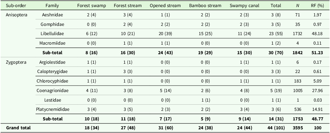
A total of 3595 individuals (51.23 % of Anisoptera and 48.77 % of Zygoptera) representing 101 species were collected in this study. They are divided amongst 10 families and 44 genera (Table 1).
Number of genera, species, abundances and relative frequencies in the different families

Table 1. Long description
A table comparing the number of genera, species, abundances, and relative frequencies in different families of Anisoptera and Zygoptera. The table has 10 rows and 10 columns. Column headers are Sub-order, Family, Forest swamp, Forest stream, Opened stream, Bamboo stream, Swampy canal, Total, N, and RF (%). Row labels include families under the sub-orders Anisoptera and Zygoptera. Row 1: Anisoptera, Aeshnidae, 2 (4), 3 (4), 1 (1), 2 (2), 2 (3), 3 (8), 71, 1.97. Row 2: Anisoptera, Gomphidae, 0 (0), 2 (4), 2 (2), 2 (2), 2 (3), 3 (5), 35, 0.97. Row 3: Anisoptera, Libellulidae, 6 (12), 10 (21), 20 (39), 15 (25), 11 (24), 23 (55), 1732, 48.18. Row 4: Anisoptera, Macromiidae, 0 (0), 1 (1), 1 (1), 0 (0), 0 (0), 1 (2), 4, 0.11. Row 5: Anisoptera Sub-total, 8 (16), 16 (30), 24 (43), 19 (29), 15 (30), 30 (70), 1842, 51.23. Row 6: Zygoptera, Argiolestidae, 1 (1), 1 (1), 0 (0), 0 (0), 1 (1), 1 (1), 6, 0.17. Row 7: Zygoptera, Calopterygidae, 1 (1), 3 (3), 0 (0), 0 (0), 0 (0), 3 (3), 22, 0.61. Row 8: Zygoptera, Chlorocyphidae, 1 (1), 1 (1), 0 (0), 0 (0), 1 (1), 1 (1), 183, 5.09. Row 9: Zygoptera, Coenagrionidae, 4 (11), 3 (8), 5 (14), 2 (6), 4 (8), 5 (19), 1005, 27.96. Row 10: Zygoptera, Lestidae, 0 (0), 0 (0), 0 (0), 1 (1), 0 (0), 1 (1), 1, 0.03. Row 11: Zygoptera, Platycnemididae, 3 (4), 3 (5), 2 (3), 2 (2), 3 (4), 3 (6), 536, 14.91. Row 12: Zygoptera Sub-total, 10 (18), 11 (18), 7 (17), 5 (9), 9 (14), 14 (31), 1753, 48.77. Row 13: Grand total, 18 (34), 27 (48), 31 (60), 24 (38), 24 (44), 44 (101), 3595, 100.
The first value represents the number of genera and in brackets the number of species.
N = abundance, RF = relative abundance in percentage.
Of the ten families identified, the most abundant were Libellulidae (48.18 % of observations across all the habitats), followed by Coenagrionidae (27.96 %). The least abundant family was Lestidae (0.03 %). Of the 101 species, the most speciose family was Libellulidae with 55 species, followed by Coenagrionidae with 19 species. The least speciose families were Argiolestidae, Chlorocyphidae and Lestidae, with one species each (Table 1).
Evaluation of the sampling effort
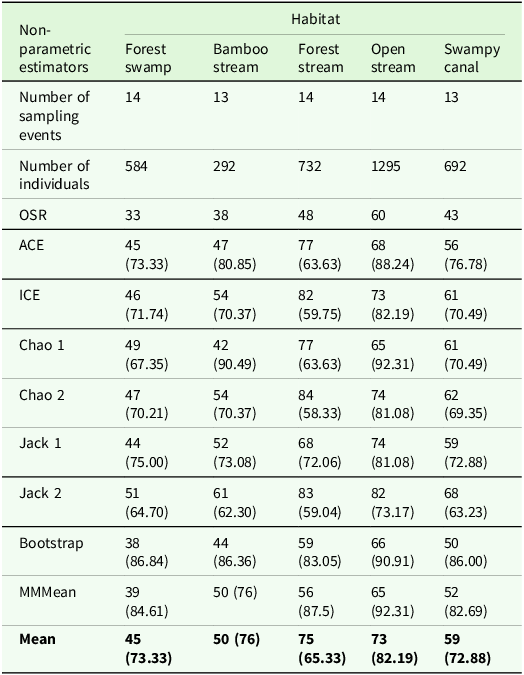
The lowest capture rate based on ICE (56.32 %) occurred in the forest stream and the highest based on MMean (92.42 %) occurred in the open stream. The estimated species richness showed that only 65.33 % of species inhabiting the forest stream were collected, while 83.56 % were collected in the open stream (Table 3). The rarefaction curves have still not reached a plateau in all habitats (Figure 3).
Rarefaction curves of the different habitats: BaSt: bamboo stream, FoSt: forest stream, FoSw: forest swamp, OpSt: open stream, SwCa: swampy canal.

Species diversity
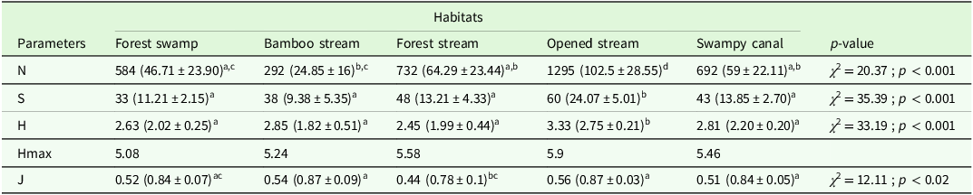
On average, the highest species richness was found in the open stream (24.07 ± 5.01) and the lowest in the forest swamp (11.21 ± 2.15). The Kruskal–Wallis analysis showed a highly significant difference in the species richness amongst the different habitats (χ 2 = 35.39; df = 4; p < 0.001). The same trend was observed with the Shannon index, which significantly varied between the sites (χ 2 = 33.19; df = 4, p < 0.001); the highest score being reported in the open stream (3.33 (2.75 ± 0.22)) and the lowest in the forest stream (2.45 (1.99 ± 0.44)). On average, the highest evenness score was found in the open stream (0.56 (0.87 ± 0.03)) and the lowest one in the forest stream (0.44 (0.78 ± 0.1)). This index also varied significantly between the habitats (χ 2 = 12.11, df = 4, p < 0.05) (Table 2). Nevertheless, the forest stream is expected to host the highest species richness, with 75 species expected to be recorded there. The lowest expected species richness is obtained in the forest swamp (45 species) (Table 3).
Diversity parameters of the different habitats

Table 2. Long description
The table presents diversity parameters for five different habitats: Forest swamp, Bamboo stream, Forest stream, Opened stream, and Swampy canal. It includes six parameters: N (number of individuals), S (species richness), H (Shannon index), Hmax (Log(S)), and J (evenness). The table has 6 rows and 6 columns, including the header row. Each habitat is compared using pairwise comparisons indicated by letters in superscript. Notable trends include variations in species richness and evenness across different habitats. For example, the Opened stream has the highest number of individuals (1295) and species richness (60), while the Forest stream has the highest Shannon index (3.33). The p-values indicate significant differences among the habitats for all parameters.
N = number of individuals, S = species richness, H = Shannon index, Hmax = Log(S), J = evenness. The letters in superscript represent pairwise comparison between types of habitats.
Non-parametric species richness estimators in the different habitats

Table 3. Long description
The table presents non-parametric species richness estimators across five different habitats: Forest swamp, Bamboo stream, Forest stream, Open stream, and Swampy canal. It includes data on the number of sampling events, number of individuals, and various estimators such as OSR, ACE, ICE, Chao 1, Chao 2, Jack 1, Jack 2, Bootstrap, MMMean, and Mean. The table has 12 rows and 6 columns. Column headers are Habitat, Number of sampling events, Number of individuals, OSR, ACE, ICE, Chao 1, Chao 2, Jack 1, Jack 2, Bootstrap, MMMean, and Mean. Row labels include the different habitats and the estimators. Each cell contains specific values related to the estimators for each habitat. Notable trends include variations in the number of individuals and the different estimators across the habitats, with the Open stream showing higher values in many categories.
In brackets are given the proportion of the observed species richness relative to the species richness estimator in question. OSR: observed species richness, ACE: abundance-based coverage estimator, ICE: incidence-based coverage estimator, Chao 1: Chao’s abundance-based richness estimator, Chao 2: Chao’s incidence-based estimator, Jack 1: first-order jackknife, Jack 2: second-order Jackknife, MMMean: Michaelis–Menten Mean.
Rényi’s diversity profiles revealed that the open stream to be the most diverse habitat overall. The bamboo stream, the forest stream and the swampy canal were proportional in their diversity indices since the profile of their diversity curves intersected with one another (Figure 4 a). On the other hand, the Rényi eveness profiles of the open stream and the bamboo stream intersect and could not be ordered. Nevertheless, they have the most evenly distributed communities (Figure 4b). The others are from the least to the most evenly distributed: forest swamp, swampy canal and forest stream.
Similarity between Odonata communities
The Bray–curtis showed that the bamboo stream and the swampy canal have the closest species composition (Figure 5). They both share 27 species (Figure 6). Of the 101 species, eight (7.92%) were present in all the five sampled habitats, notably, Copera nyansana, Elattoneura vittata, Hadrothemis defecta, Notiothemis robertsi, Orthetrum julia, Pseudagrion kibalense, Pseudagrion melanicterum and Thermochoria equivocata. Of the 94 species remaining, 45 were found in one habitat only, notably three species exclusive to the forest swamp, three to the bamboo stream, 13 to the forest stream, 26 to the open stream. No species was exclusively found in the swampy channel. The other species (49 in total) were simultaneously present in either two, three or four habitats (Figure 6).
Renyi diversity profiles of the different habitats: a) diversity profile, b) eveness profile BaSt: bamboo stream, FoSt: forest stream, FoSw: forest swamp, OpSt: open stream, SwCa: swampy canal.

Dendrogram of the similarity between the different types of habitats.

Venn diagram showing the number of specific and shared species amongst all the types of habitats.

Variation of species abundance and community structure among the habitats
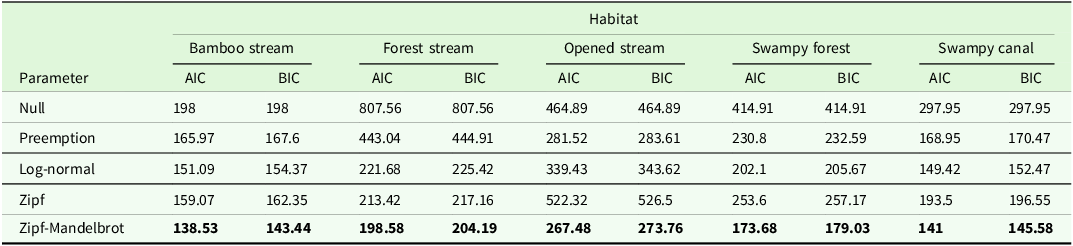
The most abundant species were Copera rufipes and Copera nyansana in the forest swamp, Orthetrum julia and Pseudagrion kiblense in the bamboo stream, Pseudagrion kibalense and Chlorocypha cyanifrons in the forest stream, Trithemis nuptialis and Ceriagrion whellani in the open stream, and, finally, Orthetrum julia and Pseudagrion kibalense in the swampy canal. The rank-abundance distribution plots are shown in Figure 7. The community structure in the five habitats followed a Mandelbrot model (Table 4).
Rank-abundance diagrams showing the distribution of Odonata fauna in the five types of habitats.

AIC and BIC values of the different models in the different habitats

Table 4. Long description
A table comparing AIC and BIC values of different models across various habitats. The table has 6 rows and 10 columns. The columns are labeled as Habitat, Parameter, Bamboo stream AIC, Bamboo stream BIC, Forest stream AIC, Forest stream BIC, Opened stream AIC, Opened stream BIC, Swampy forest AIC, Swampy forest BIC, Swampy canal AIC, and Swampy canal BIC. The rows are labeled as Null, Preemption, Log-normal, Zipf, and Zipf-Mandelbrot. Row 1: Null, 198, 198, 807.56, 807.56, 464.89, 464.89, 414.91, 414.91, 297.95, 297.95. Row 2: Preemption, 165.97, 167.6, 443.04, 444.91, 281.52, 283.61, 230.8, 232.59, 168.95, 170.47. Row 3: Log-normal, 151.09, 154.37, 221.68, 225.42, 339.43, 343.62, 202.1, 205.67, 149.42, 152.47. Row 4: Zipf, 159.07, 162.35, 213.42, 217.16, 522.32, 526.5, 253.6, 257.17, 193.5, 196.55. Row 5: Zipf-Mandelbrot, 138.53, 143.44, 198.58, 204.19, 267.48, 273.76, 173.68, 179.03, 141, 145.58.
AIC = Akaike information criterion, BIC = Bayesian information criterion. The lowest values of AIC and BIC are given in bold.
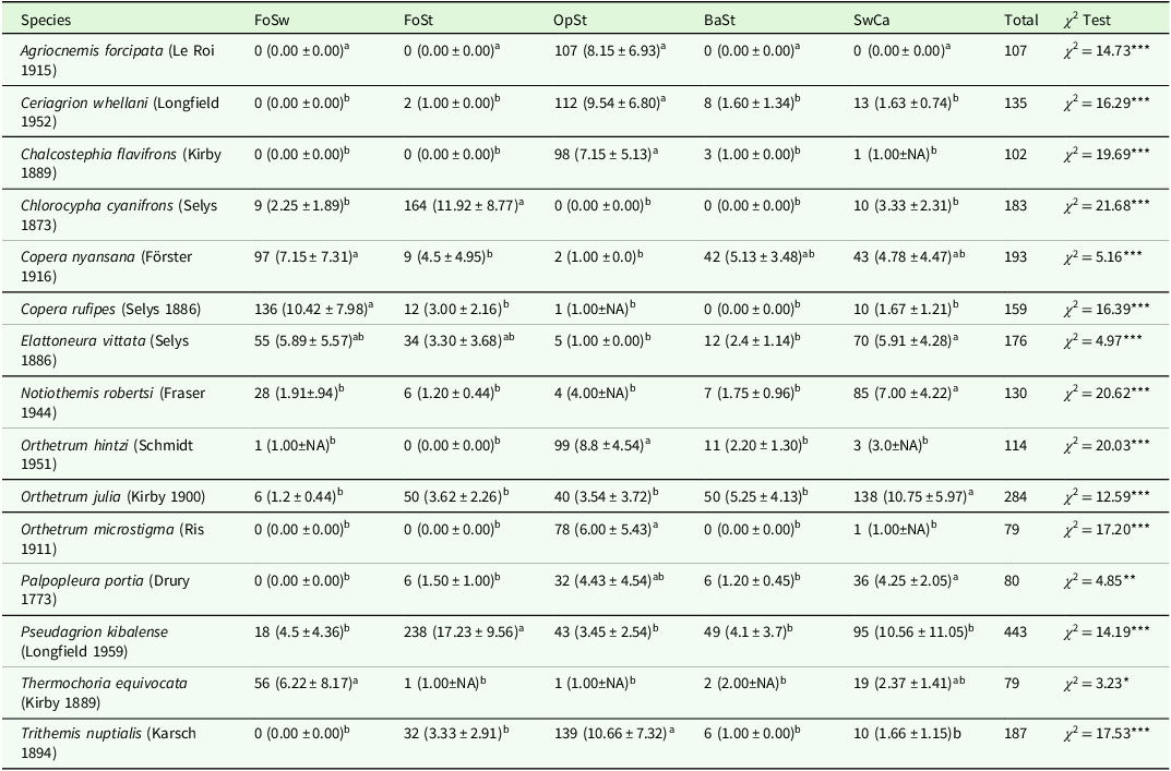
The highest abundance was recorded in the open stream with 1295 (92.5 ± 24.34) individuals followed by the forest stream (732 (52.29 ± 20.27)), the swampy canal (692 (53.23 ± 18.78)), the forest swamp (584 (41.71 ± 20.32)) and the bamboo stream with 292 (22.46 ± 14.61) specimens. The Kruskal–Wallis test showed that the average abundance varied significantly between the habitats (χ 2 = 20.37 ; p < 0.001) (Table 2). The most abundant species in all five habitats combined was Pseudagrion kibalense with 443 observations (12.32 % across all the habitats), followed by Orthetrum julia 283 (7.87 %), Copera nyansana 193 (5.37 %), Trithemis nuptialis 187 (5.20 %) and Chlorocypha cyanifrons 183 (5.09 %). The GLM analysis revealed that the abundance of each species was significantly (p ≤ 0.05) influenced by the types of habitats, showing a preference for either one or two of them.
Pseudagrion kibalense was found in all five habitat types but was significantly more abundant in forest stream (χ 2 = 14.19, p < 0.001). Orthetrum julia was found in all the habitats with an abundance significantly higher in the swampy canal (χ 2 = 12.59, p < 0.001). Copera nyansana was reported in the five habitats but significantly showed a preference for the forest swamp (χ 2 = 5.16, p < 0.001). Chlorocypha cyanifrons was not recorded in the open and bamboo streams. The habitat significantly influenced the abundance of this species (χ 2 = 21.68, p < 0.001), which was more abundant in the forest stream (Table 5, Appendix).
Comparisons of the abundances of the most abundant species between the habitats

Table 5. Long description
The table compares the abundance of various species across different habitats, including forest swamp, forest stream, open stream, bamboo stream, and swampy canal. It has 15 rows and 8 columns. The columns are labeled Species, FoSw, FoSt, OpSt, BaSt, SwCa, Total, and Chi-Squared Test. Each row lists a different species and their respective abundances in each habitat type, along with the total count and Chi-Squared Test value. Notable trends include Pseudagrion kibalense being significantly more abundant in the forest stream, Orthetrum julia in the swampy canal, and Copera nyansana in the forest swamp. Chlorocypha cyanifrons was not recorded in the open and bamboo streams but was more abundant in the forest stream.
FoSw: forest swamp, FoSt: forest stream, OpSt: opened stream, BaSt: bamboo stream, SwCa: swampy canal, N: sample size, * p < 0.05, ** p < 0.001 and ***: p < 0.0001 for significant p-values at 5 % level, ns for non-significant p-values, different letters translate the significant difference between the groups.
Dragonflies as indicator species of different habitats
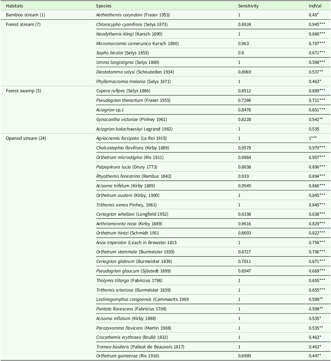
Of the 101 species collected, 37 were found to be good indicator species of the habitats: one for the bamboo stream, seven for the forest stream, five for the forest swamp and 24 for the open stream. No indicator species was found in the swampy canal. The species with the highest IndVal scores are Chlorocypha cyanifrons (IndVal = 0.95; p < 0.0001) and Neodythemis klingi (IndVal = 0.88; p < 0.0001) in the forest stream, Copera rufipes (IndVal = 0.89; p < 0.0001) and Pseudagrion thenartum (IndVal = 0.72; p < 0.0001) in the forest swamp, and Agriocnemis forcipata (IndVal = 1.00; p < 0.0001) and Chalcostephia flavifrons (IndVal = 0.97; p < 0.0001) in the open stream. Aethiothemis coryndoni (IndVal = 0.48; p < 0.05) is the only indicator species in the bamboo stream (Table 6).
IndVal statistics of indicator species in the different habitats

Table 6. Long description
A table titled ‘IndVal statistics of indicator species in the different habitats’ with four columns: Habitats, Species, Sensitivity, and IndVal. The table has 37 rows, each representing a different species and its attributes. The Habitats column lists four types: Bamboo stream, Forest stream, Forest swamp, and Opened stream, with the number of species in each habitat indicated in parentheses. The Species column lists the scientific names of the species, the Sensitivity column shows their sensitivity values, and the IndVal column displays their indicator values. Notable species include Chlorocypha cyanifrons and Neodythemis klingi in the forest stream, Copera rufipes and Pseudagion thenartum in the forest swamp, and Agriocnemis forcipata and Chalcostephia flavifrons in the opened stream. Aethiothemis coryndoni is the only indicator species in the bamboo stream.
The values in brackets after the habitats show the number of indicator species for that specific habitat. Only the species with significant probabilities are presented here. * p < 0.05, ** p < 0.001 and *** p < 0.0001.
Discussion
Our study shows that Zygoptera are significantly more abundant in the swampy forest and in the forest stream, but they are less abundant in the three other habitats, respectively, in the bamboo stream, the swampy canal and the open stream. Previous research has shown that a high proportion of Zygoptera is due to limited anthropogenic disturbance, suggesting that the swampy forest and the forest stream are the less disturbed habitats of the five (Dolný et al. Reference Dolný, Bárta, Lhota and Drozd2011, Reference Dolný, Harabiš, Bárta, Lhota and Drozd2012; Suárez-Tovar et al. Reference Suárez-Tovar, Castillo-Pérez, Sandoval-García, Schondube, Cano-Santana and Córdoba-Aguilar2022). In fact, many specialist species are recruited among Zygoptera and prefer closed canopy environments (Corbet Reference Corbet1999; Monteiro Junior et al. Reference Monteiro-Júnior, Juen and Hamada2014). Moreover, due to their small sizes, Zygoptera have restricted ecophysiological requirements; they hardly tolerate overheating and dehydration in degraded areas, restricting their biotope to relatively preserved areas where the temperatures are lower (Cai et al. Reference Cai, Ng and Ngiam2018). On the other hand, increasing anthropogenic activities tend to favour larger species, which are mostly recruited among Anisoptera (Pereira et al. Reference Pereira, Oliveira-Junior and Juen2019; Remsburg et al. Reference Remsburg, Olson and Samways2008).
We observed a significant difference in the species richness, with the highest found in open stream. Bried and Ervin (Reference Bried and Ervin2005), Clausnitzer (Reference Clausnitzer2003), Dijkstra and Lempert (Reference Dijkstra and Lempert2003), Monteiro Júnior et al. (Reference Monteiro Júnior, Couceiro, Hamada and Juen2013), Seidu et al. (Reference Seidu, Danquah, Nsor, Amaning and Lancaster2017) and Worthen and Chamlee (Reference Worthen and Chamlee2020) also reported a higher species diversity of dragonflies in opened water bodies compared to more closed ones. Although open areas may support higher species diversity, this diversity may be of lower conservation value than the lower diversity found in forest habitats, because forests can contain some specialists or rare species (Clausnitzer Reference Clausnitzer2003). Indeed, the opened stream may act as an ecological trap due to the high quantity of light reflected by the water surface. Odonata principally use visual cues for habitat selection (Wildermuth Reference Wildermuth1994), and the polarized light reflected by water surfaces can misconduct many species that will hover and oviposit in unsuitable habitats for them, as the eggs and larvae are unable to develop and survive (Cezário et al. Reference Cezário, Lopez, Datto-Liberato, Bybee, Gorb and Guillermo-Ferreira2025; Horváth et al. Reference Horváth, Malik, Kriska and Wildermuth2007). On the other side, in forested ecosystems where the light is reduced, species found there are more likely to find more suitable habitats for their development (Dijkstra and Clausnitzer Reference Dijkstra, Clausnitzer and Cordero Rivera2006).
In all habitats, none of the species richness estimators have a value of 100%, and the rarefaction curves have not reached a plateau yet, suggesting that more sampling effort is still required to reach the maximum species richness. Despite the low species richness observed in forest streams, the estimators showed that the habitat is expected to host the highest species richness of the five habitats. In tropical regions, Odonata species richness is higher in forests than in any other ecosystems (Dijkstra Reference Dijkstra, Clausnitzer and Cordero Rivera2006) due to the high diversity of habitats and the most stable conditions which permit them to reproduce all throughout the year (Kalkman et al. Reference Kalkman, Clausnitzer, Dijkstra, Orr, Paulson and Van Tol2008). Estimating real species richness of habitats is very useful in assessment and monitoring animal populations as it gives the possibility to compare the habitats at different levels (Oertli Reference Oertli and Cordoba-Aguilar2008). The low species richness observed in the forest stream here can be explained by the limited detectability of odonates due to the relative shade (Oppel Reference Oppel2006).
The Mandelbrot distribution of the Odonata communities in the five habitats reflects environmental and ecological conditions that are consistent with incompletely sampled communities (Ulrich et al. Reference Ulrich, Ollik and Ugland2010). This model characterizes communities where the most abundant species are the first to have colonized the sites and have large ecological preferences when the least abundant are more specialized to the habitat (Girard-Buttoz et al. Reference Girard-Buttoz, Ouin, Tessier, Gergaud, Sarthou and Balent2008). This model belongs to the log-series models, which suggest moderately disturbed communities (Gray Reference Gray, Gee and Giller1987) and communities where there is a very high proportion of rare species (Fisher et al. Reference Fisher, Corbet and Williams1943). In such communities, a great part of the resources are distributed between few species, the most abundant ones, implying a limited competition in Odonata communities of Minko’o.
The Mandelbrot distribution also characterizes complex communities, and the higher the number of species, the more complex the community (Marage and Bertrand Reference Marage and Bertrand2012). The highest number of singletons is noted in the forest stream and the lower number is found in the bamboo stream. This suggests that the forest stream is the most stable. This can be explained by the limited anthropogenic activities there. The bamboo stream, in contrast, despite the limited human activity is the least stable. The invasion by the invasive species Bambusa vulgaris Schrad. ex J.C.Wendl. (GISD 2025) is probably influencing the dragonfly community, which could disappear if the bamboos are not removed. Nevertheless, increasing the sample sizes and taking into account the ecology of the species are necessary to confirm these hypotheses. Indeed, the habitat specificity, the presence of vagrants or occasional species and the detectability of species (some species may appear rarer than it actually is in nature) can justify the great number of singletons in communities (Magurran and Henderson Reference Magurran, Henderson, Magurran and McGill2010).
Pseudagrion kibalense and O. julia were the most abundant species. They were recorded in all five habitats, but with a significantly higher abundance in the forest stream for P. kibalense and the swampy canal for O. julia. The two species are widespread and can colonize a broad range of forest habitats, especially streams with low water flow and sandy or gravel-like substrate for P. kibalense; while O. julia prefers shaded streams in gallery forests (Dijkstra Reference Dijkstra2017). Chlorocyphidae and Lestidae are represented by one species each, Chlorocypha cyanifrons and Lestes cf. uncifer. Of the 22 individuals of Gynacantha bullata recorded, sixteen of them were collected at dusk, showing its crepuscular behaviour as reported before by Clausnitzer (Reference Clausnitzer1999) and Corbet (Reference Corbet1962). Crepuscular species may also appear during the day, especially when the light intensity decreases, and are not tolerant to high temperatures and low humidity; this generally happens at the end of the day (Corbet Reference Corbet1962).
The highest number of indicator species was observed in the open stream. This suggests that this habitat is unique compared to the others (Vilches et al. Reference Vilches, De Cáceres, Sánchez-Mata and Gavilán2013). In fact, this habitat is not shaded at all compared to the other ones and is experiencing a lot of perturbations from human activities, including fishing, and receives a lot of chemicals from washing activities (clothes, cars, motorbikes and dishes). The indicator species from this habitat are also known to be generalists and are considered heliophilic or stagnant-water species, notably Chalcostephia flavifrons and Palpopleura lucia (Seidu et al., Reference Seidu, Nsor, Danquah, Tehoda and Oppong2019). The aforementioned species are also associated with natural ponds with a lot of tall grasses and reeds on the bank (Samways and Simaika Reference Samways and Simaika2016). In the forest stream, seven species were identified as biological indicators of the forest streams. Our observations were similar to those of Dijkstra and Lempert (Reference Dijkstra and Lempert2003), who found that Neodythemis klingi highly depends on forest cover and is strongly related to small streams.
In summary, our results highlight that Odonata assemblages significantly vary across the habitats. This confirms that odonates represent a cost-effective tool for biomonitoring and environmental assessments in Central Africa. Our current research also reinforces the necessity of consistent sampling in order to document the odonates biodiversity in Central Africa, which is still amongst the least explored regions on the continent. In fact, the species richness estimators show that up to 45% of the diversity in some habitats is still to be reported. This research also highlights the urgency of preserving and restoring original habitats. We recorded Neurolestes trinervis, which is reported as “Vulnerable” on the IUCN (International Union for the Conservation of Nature) Red List. Actions should be taken to prevent further degradation of the environment.
Supplementary material
The supplementary material for this article can be found at https://doi.org/10.1017/S0266467426100728.
Acknowledgements
The authors would like to thank Klaas-Douwe B. Dijkstra for his immense advice and the local communities of Minko’o for allowing us to access their plantations to carry out this work.
Financial support
This research received no specific grant from any funding agency, commercial or not-for-profit sectors.
Competing interests
The authors declare none.







 Open access

