1. Introduction
Surface roughness can have a dramatic effect on the dynamics of turbulent boundary layers (Jiménez Reference Jiménez2004; Flack & Schultz Reference Flack and Schultz2014). It is typically assumed that the effects of roughness are confined to the roughness layer (Castro Reference Castro2007; Flack, Schultz & Connelly Reference Flack, Schultz and Connelly2007; Amir & Castro Reference Amir and Castro2011); however, recently it has been observed that large secondary motions in the mean flow can form naturally over rough surfaces and impact even the outer structure of the boundary layer. Mejia-Alvarez & Christensen (Reference Mejia-Alvarez and Christensen2013) and Barros & Christensen (Reference Barros and Christensen2014) observed low- and high-momentum pathways occupied by large secondary swirling motions in the mean flow over the irregular surface topology of a replica of a damaged turbine blade. Reynolds et al. (Reference Reynolds, Hayden, Castro and Robins2007) observed that similar secondary flows form over repeating arrays of cubes in a wind tunnel, and Wang & Cheng (Reference Wang and Cheng2006) observed the formation of these secondary flows in open channel flow with longitudinal bedforms consisting of smooth and pointed ridges. Similar structures were also observed by Nugroho, Hutchins & Monty (Reference Nugroho, Hutchins and Monty2013) over a surface with converging–diverging riblets, which guided the flow into high-momentum pathways near the wall and in turn created large secondary swirling motions. Numerical simulations by Willingham et al. (Reference Willingham, Anderson, Christensen and Barros2014) of the flows over spanwise-alternating roughness demonstrated that the size and spacing of these secondary motions are of the order of the boundary layer thickness and are not particularly sensitive to the roughness height, but have some sensitivity to the width of the roughness elements. The existence of these large secondary motions clearly illustrates that the effect of the roughness topology on the flow is not necessarily confined to the immediate vicinity of the surface (i.e. the roughness sublayer) but under certain conditions can impact the entire extent of the turbulent boundary layer.
In this study, we intend to specifically investigate the conditions necessary for the formation of large-scale secondary flows by studying their sensitivity to the spanwise spacing of the roughness features. We hypothesize that large secondary vortices only form when the spacing of roughness elements is comparable to the boundary layer thickness. To test this idea, we measure the flow field over five systematically defined surfaces having streamwise strips of elevated roughness elements with varying spanwise spacing.
2. Experimental procedures
Experiments were performed in the University of Southampton’s suction wind tunnel using Lego bricks to form the roughness elements, similarly to previous experiments in the same facility (Placidi & Ganapathisubramani Reference Placidi and Ganapathisubramani2015). The wind tunnel has a working section 4.5 m long with a
 $0.9~\text{m}\times 0.6~\text{m}$
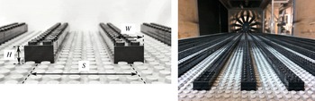
cross-section. In this study, strips of Lego bricks having a width of
 $W=16~\text{mm}$
and height of
 $H=9.6~\text{mm}$
were aligned with the flow direction and extended over the full 4.5 m length of the wind tunnel test section (see figure 1). These dimensions do not include the array of ‘bumps’ used to connect the pieces together, which have a diameter of 4.8 mm and a height of 1.7 mm and which covered the floor of the wind tunnel uniformly. The centre-to-centre spacing,
 $S$
, of the elevated strips was varied to test five cases with ratios of
 $S/W=2$
, 3, 6, 8 and 12. We apply the convention that
 $x,y,z$
are the streamwise, wall-normal and spanwise directions, and
 $U,V,W$
are the corresponding velocities in those directions. Time-averaged mean values are denoted by an overline, as for example
 $\overline{U}$
, while the fluctuations about the mean are denoted by lower case, as for example
 $u$
, and values that are averaged across the span and in time are denoted by angle brackets, as for example
 $\left\langle U\right\rangle$
.
Illustrations of the surface topology, with roughness strips aligned in the streamwise direction.

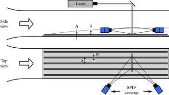
Measurements of the velocity field that developed over the surface were acquired using stereo particle image velocimetry (PIV) in a cross-section normal to the flow direction at a position 4 m downstream of the leading edge, as illustrated in figure 2. This development distance is nearly double the suggested length of
 $20{\it\delta}$
to ensure fully developed conditions in rough-wall turbulent boundary layers (Antonia & Luxton Reference Antonia and Luxton1971; Castro Reference Castro2007), where
 ${\it\delta}$
is the boundary layer thickness and is reported below in § 3.1. A 200-15PIV Nd:YAG laser by Litron Lasers illuminated the measurement plane and the flow was seeded using a Magnum 1200 fog machine. Particle images were recorded using two LaVision Imager LX 29MP cameras, fitted with lenses having a focal length of 200 mm and an aperture of
 $f5.6$
. The cameras were positioned on either side of the measurement plane at angles of approximately
 $\pm 35^{\circ }$
from the measurement plane and fitted with Scheimpflug adapters to accommodate the oblique viewing angle. The coordinate system mapping function for the two cameras was determined using a third-order polynomial fit to images of a double-sided dual-plane calibration target aligned with the measurement plane before the experiment.
Schematic of the experimental set-up in the wind tunnel. Measurements of the velocity field were obtained in a spanwise cross-section of the flow using stereo PIV (SPIV).

In all of the test cases, the free stream velocity was set to
 $U_{\infty }=15~\text{m}~\text{s}^{-1}$
. For each case, a total of 1500 image pairs were acquired with an image pair separation time of
 $15~{\rm\mu}\text{s}$
at a rate of 2 Hz, which was slow enough such that each measurement could be considered independent. Vectors were determined with LaVision’s DaVis 8.2.2 software, using window sizes of
 $32~\text{pixel}\times 32~\text{pixel}$
with 50 % overlap, resulting in a resolution of one vector per 0.9 mm. The instantaneous vector maps were subsequently post-processed in MATLAB to detrend the mean vector maps, which contained a subtle spanwise bias which could have been due to a slight misalignment of the calibration plate with the laser plane. The magnitude of this correction was approximately
 $0.2~\text{m}~\text{s}^{-1}$
, which is of the order of the uncertainty of the PIV measurement and corresponds to approximately 1 % of
 $U_{\infty }$
.
3. Results
3.1. Turbulence properties
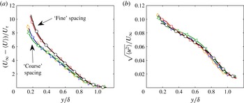
Profiles of the mean streamwise velocity in defect form and the root-mean-square streamwise velocity fluctuations in the boundary layer formed over each of the five surfaces are presented in figure 3. Despite the different spacings of the roughness elements, the 99 % boundary layer thickness for all of the flows is
 ${\it\delta}=108\pm 1~\text{mm}$
, which results in
 ${\it\delta}/H=11.3\pm 1\,\%$
. Although the profiles of the fluctuations appear to collapse across all cases (figure 3
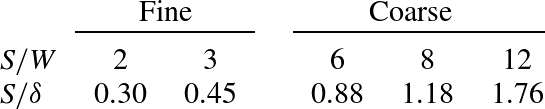
b), the mean profiles in figure 3(a) diverge into two groups near the wall. We may distinguish the two different groups as those with spanwise spacing much less than the boundary layer thickness, i.e. ‘fine’ spacing, and those with spacing comparable to or larger than
 ${\it\delta}$
, i.e. ‘coarse’, as summarized in table 1. The cases with fine spacing have a larger deficit near the wall, whereas the cases with coarse spacing have fuller profiles. This suggests that coarser spanwise spacings have improved near-wall mixing, bringing in a larger amount of high-momentum fluid to the near-wall region, thereby resulting in a fuller profile.
Profiles of (a) the mean velocity deficit and (b) the root-mean-square velocity fluctuations averaged across the span for
 $S/{\it\delta}=0.30$
(○), 0.45 (▫), 0.88 (◃), 1.18 (▹) and 1.76 (♢). Markers are spaced every 15 data points for clarity.

Summary of the five test cases in the current study.

The skin-friction velocity,
 $U_{{\it\tau}}$
, was determined from the plateau of the measurements of the Reynolds stress,
 $-\overline{uv}$
, near the wall (Amir & Castro Reference Amir and Castro2011). Although the Reynolds stress varies at different spanwise locations, the plateau in the spanwise-averaged stress is consistent between all the different test cases, resulting in
 $U_{{\it\tau}}=0.63~\text{m}~\text{s}^{-1}\pm 10\,\%$
. Maps of the Reynolds stresses are presented later on in figure 6 and the significance of their spanwise variations will be discussed in greater detail below. The Karman number can then be defined as
 $\mathit{Re}_{{\it\tau}}={\it\delta}U_{{\it\tau}}/{\it\nu}$
, and this is in the range
 $4200\pm 400$
for all the test cases.
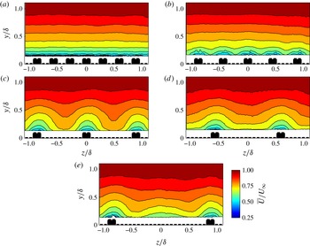
Contour maps of the mean streamwise velocity above the roughness elements for the surfaces with
 $S/{\it\delta}=$
(a) 0.30, (b) 0.45, (c) 0.88, (d) 1.18 and (e) 1.76. The cross-sections of the roughness elements are drawn to scale for reference.

3.2. Maps of the mean streamwise velocity
Despite the similarities of the mean profiles, the maps of the mean flow field demonstrate strong spanwise heterogeneities that depend on the surface roughness spacing. These differences are clearly observed in the contour maps of the mean streamwise velocity, which are plotted in figure 4. For the cases with fine spacing, these spanwise variations are confined to the roughness sublayer (
 $y<3H$
), above which the standard deviations of the spanwise fluctuations decrease below 1 % of
 $U_{\infty }$
. In contrast, the surfaces with coarse spacing create spanwise variations that extend to the outer region of the boundary layer. Regions of lower velocity, corresponding to low-momentum pathways, are in the vicinity of the elevated roughness strips, whereas, in general, the unhindered flow away from these regions forms high-momentum pathways between the roughness elements. These spanwise variations in the streamwise velocity are most accentuated for the case with surface spacing closest to the boundary layer width (
 $S/{\it\delta}=0.88$
), presented in figure 4(c). For this case, the mean velocity exhibits peak-to-peak variations of 18 % at
 $y/{\it\delta}=0.25$
and only decreases to the same level of uniformity as the fine cases for
 $y/{\it\delta}>0.75$
. This confirms that the spacing of the roughness is a key parameter in controlling the size and influence of these low- and high-momentum pathways and that by altering nothing but the spacing of the roughness elements, large perturbations to the structure of the mean velocity field may be created.
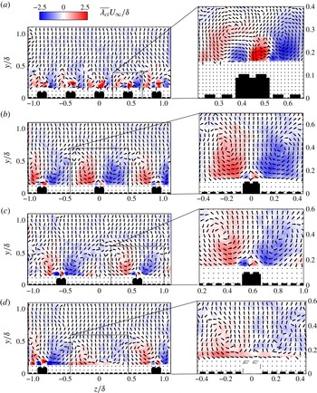
Maps of the mean signed swirling strength for
 $S/{\it\delta}=$
(a) 0.45, (b) 0.88, (c) 1.18 and (d) 1.76. The secondary flows that develop over the roughness elements are magnified in (a–c), and in (d) the tertiary flow that forms between the secondary vortices is magnified, where a dashed outline indicates the ‘virtual’ roughness element representing the harmonic corresponding to the wavelength
 ${\sim}{\it\delta}$
. It should be noted that not all vectors are shown in these maps for clarity.

3.3. Large-scale secondary flows
The large-scale secondary flows associated with these variations in the streamwise velocity can be easily observed in maps of the mean signed swirling strength and mean in-plane velocity vector fields presented in figure 5. The mean signed swirling strength was calculated as the ensemble average of the instantaneous swirling strength maps, multiplied by the sign of the vorticity, as in Anderson et al. (Reference Anderson, Barros, Christensen and Awasthi2015), in order to indicate both the strength and the direction of rotation of the regions of swirl. For the cases with coarse spacing, large secondary vortices can be clearly observed. The secondary flow consists of a pair of counter-rotating vortices, which are formed on either side of the elevated roughness strips. These are associated with regions of strong upwelling over the elevated regions and wide downdraughts in the valleys. The downdraughts carry with them high velocity from the outer boundary layer and are consistent with the descriptions of high-momentum pathways; similarly, the regions over the elevated roughness correspond to low-momentum pathways. In these measurements, the locations of the low-momentum pathways always occur directly above the elevated roughness elements, which is in contrast to some previous observations; however, we discuss these differences in § 4.1.
The case with a spacing of
 $S/{\it\delta}=0.45$
is an excellent example of what happens in the limit of the fine-spacing regime (see figure 5
a). In this case, a small pair of counter-rotating vortices (whose sense of rotation is opposite to that of the secondary flows) appear directly above each roughness element, corresponding to a small downwash. These small vortices in fact appear in every case; however, for the coarse spacings, the large secondary vortices dwarf these small vortices. If one looks closely, similar small vortices may also be observed in the vorticity maps by Anderson et al. (Reference Anderson, Barros, Christensen and Awasthi2015). In this limit case with
 $S/{\it\delta}=0.45$
, the larger secondary vortices still appear, flanking these smaller vortices; however, the diameter of the larger secondary vortices is nearly the same as that of the small vortices that occur above the roughness element, making them difficult to distinguish in the measurements, and having minimal effect on the mean velocity field. The fact that the sizes of these structures are contained within the roughness sublayer is consistent with the observation that the spanwise variations in the mean velocity maps are also limited to the roughness sublayer. These structures occurred at even finer scales in the case with the finest surface spacing, which we omitted from figure 5 because it did not exhibit any discernible structure, consistent with the fact that it also did not exhibit large spanwise variations in the mean velocity map.
It appears, therefore, that the size of the secondary vortices is controlled by the roughness spacing, forcing the diameter of each vortex to be approximately one-half of the roughness spacing. However, this trend stops at the limit when the spacing equals the boundary layer thickness, at which point the strength and size of the vortices do not grow any further. The diameter of the large-scale secondary flows was never observed to exceed
 ${\it\delta}$
, perhaps because the vertical distance up to which these secondary motions can grow is limited by the boundary layer thickness, and therefore so is their spanwise length scale.
In the case when the spacing exceeds the boundary layer thickness (
 $S/{\it\delta}=1.76$
), the flow develops a large-scale tertiary flow, comprising another pair of counter-rotating vortices (similar to the secondary flow) located at the centres of the valleys between the elevated roughness strips. The strength of these tertiary vortices is roughly half that of the secondary vortices. It appears that as the spanwise spacing increases beyond
 ${\it\delta}$
, large-scale tertiary flows start to appear at roughly
 ${\it\delta}$
spacing, and presumably will continue to get weaker as the spacing increases further. This observation demonstrates the significance of the boundary layer thickness to the roughness width in the formation of secondary and tertiary flows.
3.4. Maps of Reynolds stresses
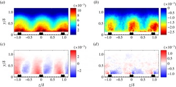
Representative maps of the normal and turbulent Reynolds stresses that occur in conjunction with these secondary/tertiary flows are presented in figure 6. We only illustrate the case that exhibits the largest secondary flow (
 $S/{\it\delta}=0.88$
); however, similar patterns were observed in the flows over each of the surfaces with coarse roughness. The patterns of the turbulent Reynolds stresses are similar to those observed in the large-eddy simulations (LES) presented by Anderson et al. (Reference Anderson, Barros, Christensen and Awasthi2015). The variance of the streamwise velocity
 $\overline{uu}$
is a maximum in the vicinity of the elevated roughness, and particularly near the corners of the roughness elements at the interface of the small vortices and large secondary flows that occur in the low-momentum pathways. The Reynolds shear stress
 $-\overline{uv}$
is also a maximum near the elevated roughness, but exhibits high values that extend to nearly half the boundary layer thickness, following the strong updraughts that occur above the elevated surfaces. Anderson et al. (Reference Anderson, Barros, Christensen and Awasthi2015) also observed peaks of
 $-\overline{uv}$
at the base of the high-momentum pathways (which occurred here in the valleys between the roughness strips); however, we do not capture this region very clearly in our measurements, and it is unclear whether such a region exists in figure 6(b). The transverse shear stresses
 $\overline{uw}$
and
 $\overline{vw}$
are very clearly symmetric and periodic with the roughness spacing, in accordance with the directionality of the mean spanwise velocity
 $\overline{W}$
imposed by the large secondary flows. Anderson et al. (Reference Anderson, Barros, Christensen and Awasthi2015) stressed the importance of the spanwise gradients of the shear stresses and the role they play in driving the secondary vortices, which were interpreted as Prantl’s secondary flows of the second kind; the fact that the stresses behave similarly in the current measurements to their results supports this interpretation. Again, we note that the main difference between these observation and those of Anderson et al. (Reference Anderson, Barros, Christensen and Awasthi2015) is the fact that the locations of the low-momentum pathways always occur directly above the elevated roughness elements, whereas in the LES these occurred over what they referred to as ‘high’ roughness; however, we attempt to explain these differences in § 4.1.
Maps of the turbulent stresses over the roughness spaced by
 $S/{\it\delta}=0.88$
, which exhibited the largest secondary flows: (a)
 $\overline{uu}/U_{\infty }^{2}$
, (b)
 $\overline{uv}/U_{\infty }^{2}$
, (c)
 $\overline{uw}/U_{\infty }^{2}$
, (d)
 $\overline{vw}/U_{\infty }^{2}$
.

4. Discussion
4.1. On the locations of low- and high-momentum pathways
In the current measurements, for the cases with coarse spacing where large secondary flows develop, the low-momentum pathways always occur directly above the elevated roughness elements and the high-momentum pathways occur in the valleys between them. This is in contrast to some previous experiments and simulations, and at this point we would like to address the reasons for these differences. In the current experiments, the surface topology is constant in the streamwise direction, and the locations of these pathways are constrained by the topology as the flow develops downstream. One could imagine that in the cases with coarse spacing, boundary layers grow over the top and sides of the elevated roughness features, blocking part of the flow area, retarding the local fluid around this blockage and creating low-momentum zones which persist downstream. In the valleys between the elevated strips, the flow is less inhibited and forms a high-momentum pathway. This is consistent with previous studies over ridged longitudinal bedforms by Wang & Cheng (Reference Wang and Cheng2006). Therefore, why do the locations differ in some other studies?
In experimental studies of the flow over the irregular surface of a damaged turbine blade, Barros & Christensen (Reference Barros and Christensen2014) (and Anderson et al.
Reference Anderson, Barros, Christensen and Awasthi2015) found that low-momentum pathways were systematically positioned above regions with relatively recessed surfaces, and they argued that the gradient of the surface elevation could play a role in organizing the secondary flows. However, over a three-dimensional surface such as that which was considered in their experiment, boundary layers do not have the opportunity to grow significantly over the elevated roughness features before the topology changes. Although the surface appears to have roughness features that are elongated in the streamwise direction, the reality is that there are repeating hills and valleys all along the streamwise direction. The small elevated hills would actually cause a local acceleration of the fluid over them, due to the pressure gradient they impose. This would result in high-momentum pathways generated over elevated roughness features. If the roughness feature persisted downstream (instead of forming hills and valleys), the flow would eventually be deviated, forming a low-momentum pathway. Therefore, the streamwise continuity of the surface topology is an important factor in the locations of these pathways. One would expect that small gaps in the streamwise continuity of long ridges would not significantly alter the flow, as the bulk flow would skim over such gaps. Considering that the separation region behind a cube is known to be approximately
 $4{-}5H$
(Castro & Robins Reference Castro and Robins1977), one may predict that surfaces with streamwise roughness strips having gaps of less than
 $4{-}5H$
would act like continuous strips and exhibit low-momentum pathways coincident with the elevated roughness strips, whereas surfaces with longer gaps would behave more like the irregular surface observed by Barros & Christensen (Reference Barros and Christensen2014).
The numerical simulations of Willingham et al. (Reference Willingham, Anderson, Christensen and Barros2014) (and Anderson et al.
Reference Anderson, Barros, Christensen and Awasthi2015) considered continuous streamwise-aligned surface roughness, and naturally the question becomes, why did this study also observe low-momentum pathways over the ‘low’ roughness regions? In this case, we attribute the difference to the fact that the simulations did not resolve the roughness topology. The authors reproduced the topology by changing
 ${\rm\Delta}U^{+}$
(which is the downward shift in the logarithmic region compared with a smooth wall). Their ‘high’ roughness was simulated by increasing
 ${\rm\Delta}U^{+}$
, which would have the effect of increasing the velocity gradient at the wall, bringing higher momentum flow towards the wall. This would be similar to the flow that would form over a region with recessed roughness in our experiments. Similarly, reducing
 ${\rm\Delta}U^{+}$
would result in a slower flow, similar to that over elevated roughness in our experiments. Therefore, the ‘low’ roughness regions in the simulations are more akin to the flow created over elevated roughness in the experiments, and likewise ‘high’ roughness to recessed regions. With this in mind, the current results are consistent with the simulations.
4.2. Conditions for large-scale secondary flows
In light of these results, we may speculate that a necessary condition for the formation of these large-scale secondary vortex structures is that the spanwise spacing of the wall roughness is sufficiently coarse (
 $S/{\it\delta}\gtrsim 0.5$
). When the roughness spacing is too fine, any secondary motions do not have the room to grow and are confined to the roughness sublayer. The secondary flows are accentuated the most when the roughness spacing has a period close to the boundary layer thickness; however, larger spacings also generate similar secondary flows, but these motions become weaker due to the formation of tertiary flows between the secondary flows. Previous studies by Willingham et al. (Reference Willingham, Anderson, Christensen and Barros2014) have shown that the roughness height does not have a strong effect and that the width of the strips has only a small influence. Specifically, they tested cases where the ratio of the high and low roughness strips ranged two orders of magnitude from 2 to 900 and the widths of the strips ranged from 0.2 to
 $1.0{\it\delta}$
and found that all the cases produced these types of large secondary motions. Therefore, the spanwise spacing appears to have the most significant effect. We found that all the previous studies we reviewed in the literature that observed large secondary flows do indeed satisfy these requirements. All of the numerical simulations of Willingham et al. (Reference Willingham, Anderson, Christensen and Barros2014) had a spacing of
 $S/{\it\delta}={\rm\pi}$
. The longitudinal bedforms studied by Wang & Cheng (Reference Wang and Cheng2006) were spaced by approximately twice the channel depth. Even the converging–diverging riblet-type surface roughness studied by Nugroho et al. (Reference Nugroho, Hutchins and Monty2013) had a spanwise period ranging from
 $S/{\it\delta}=2$
to 2.7.
The only possible exception that we found in the literature was the experimental study by Reynolds et al. (Reference Reynolds, Hayden, Castro and Robins2007), which observed secondary flows over various repeating surface patterns with periods smaller than the boundary layer thickness. They explained that these structures appeared to be Klebanoff-type modes associated with transition which were organized by the periodicity of the surface roughness. However, they noted that the magnitudes of these secondary flows decreased downstream, as would be expected of transitional phenomena and in contrast to the secondary flows produced by coarse spacings which persist far downstream. Furthermore, they found that when the spacing was finer than
 $S/{\it\delta}\lesssim 0.2$
the secondary flows were no longer detectable. This is consistent with our conclusions and suggests that for short distances the threshold spacing for the development of these secondary flows is reduced in comparison to the far-downstream limit where the spacing should be near
 ${\it\delta}$
for large secondary flows to flourish.
For a surface with irregular roughness, a measure of the periodicity can be determined by inspection of the cross-stream autocorrelation function of the surface height. In order to comment on the experimental findings of Barros & Christensen (Reference Barros and Christensen2014), we have digitized their surface and calculated the spanwise autocorrelation function. We found that in addition to the initial correlation region extending to approximately
 ${\rm\Delta}z/{\it\delta}=0.2$
, which corresponds to the average width of the roughness features, it also had local peaks at
 ${\rm\Delta}z/{\it\delta}=0.63$
and 1.18. These secondary peaks reveal the spanwise spacing of the roughness features, which could be responsible for the development of these large secondary flows. This demonstrates the caution required when designing flows over rough surfaces, because elements with a period near
 ${\it\delta}$
may develop large secondary recirculating regions that disrupt the natural development of the boundary layer.
5. Conclusions
This study shows that the presence of large secondary flows is directly related to the spanwise spacing of the surface roughness. These secondary flows consist of large counter-rotating recirculation zones that flank the roughness features and are associated with low- and high-momentum pathways. These secondary flows cause large perturbations to the structure of the mean velocity field, resulting in significant spanwise deviations that extend beyond the roughness sublayer to over 75 % of the boundary layer thickness.
We determined that a necessary condition for the development and persistence of these secondary vortex structures is that the wall roughness is sufficiently coarse (
 $S/{\it\delta}\gtrsim 0.5$
), and when the roughness spacing is too fine, any spanwise variations are confined to the roughness sublayer. The strength of these secondary vortices appears to be maximized when the spacing is comparable to boundary layer thickness; however, larger spacings also generate secondary flows as well as tertiary flows, which together maintain a
 ${\it\delta}$
-scale spacing. Because these secondary flows have such a large impact on the structure of the boundary layer and can be created so easily by modifying the surface topology, these flows have important consequences for near-wall mixing, drag reduction and flow control.
Acknowledgements
We gratefully acknowledge the financial support from the European Research Council (ERC grant agreement no. 277472), EPSRC (grant ref no: EP/I037717/1) and the European Commission (project ref no. 656081). We also thank our friends and colleagues who helped assemble all the Lego in the wind tunnel.