INTRODUCTION
Fossil fuel combustion comprises the largest anthropogenic CO2 source on Earth. It accounted for approximately 7.0 GT yr–1 in 2000, and increased rapidly to over 9.8 GT yr–1 in 2014 (Marland et al. Reference Marland, Boden and Andres2006; Raupach et al. Reference Raupach, Marland, Ciais, Le Quéré, Canadell, Klepper and Field2007; Le Quéré et al. Reference Le Quéré, Moriarty, Andrew, Canadell, Sitch, Korsbakken, Friedlingstein, Peters, Andres, Boden, Houghton, House, Keeling, Tans, Arneth, Bakker, Barbero, Bopp, Chang, Chevallier, Chini, Ciais, Fader, Feely, Gkritzalis, Harris, Hauck, Ilyina, Jain, Kato, Kitidis, Klein Goldewijk, Koven, Landschützer, Lauvset, Lefèvre, Lenton, Lima, Metzl, Millero, Munro, Murata, Nabel, Nakaoka, Nojiri, O’Brien, Olsen, Ono, Pérez, Pfeil, Pierrot, Poulter, Rehder, Rödenbeck, Saito, Schuster, Schwinger, Séférian, Steinhoff, Stocker, Sutton, Takahashi, Tilbrook, van der Laan-Luijkx, van der Werf, van Heuven, Vandemark, Viovy, Wiltshire, Zaehle and Zeng2015). From 1870 to 2014, approximately 400 GT of carbon were released to the atmosphere from the consumption of fossil fuels and cement production (Le Quéré et al. Reference Le Quéré, Moriarty, Andrew, Canadell, Sitch, Korsbakken, Friedlingstein, Peters, Andres, Boden, Houghton, House, Keeling, Tans, Arneth, Bakker, Barbero, Bopp, Chang, Chevallier, Chini, Ciais, Fader, Feely, Gkritzalis, Harris, Hauck, Ilyina, Jain, Kato, Kitidis, Klein Goldewijk, Koven, Landschützer, Lauvset, Lefèvre, Lenton, Lima, Metzl, Millero, Munro, Murata, Nabel, Nakaoka, Nojiri, O’Brien, Olsen, Ono, Pérez, Pfeil, Pierrot, Poulter, Rehder, Rödenbeck, Saito, Schuster, Schwinger, Séférian, Steinhoff, Stocker, Sutton, Takahashi, Tilbrook, van der Laan-Luijkx, van der Werf, van Heuven, Vandemark, Viovy, Wiltshire, Zaehle and Zeng2015). This accelerated trend began centuries ago and the mole fraction of atmospheric CO2 has been steadily increasing since the Industrial Revolution (IPCC 2007). Therefore, monitoring atmospheric CO2 sources is increasingly important in the interests of establishing controllable strategies and implementing greenhouse gas regulations (Djuricin et al. 2007).
The radiocarbon concentration of atmospheric CO2 can provide valuable information about its sources (Levin and Hesshaimer Reference Levin and Hesshaimer2000; Takahashi et al. Reference Takahashi, Konohira, Hiyama, Minami, Nakamura and Yoshida2002; Kuc et al. Reference Kuc, Rozanski, Zimnoch, Necki and Korus2003; Levin et al. Reference Levin, Kromer, Schmidt and Sartorius2003, Reference Levin, Hammer, Kromer and Meinhardt2008; Turnbull et al. Reference Turnbull, Miller, Lehman, Tans, Sparks and Southon2006; Levin and Karstens Reference Levin and Karstens2007; Levin and Rodenbeck Reference Levin and Rodenbeck2008). CO2 from the combustion of fossil fuels contains no 14C because the half-life of 14C (5700±30 yr) is much less than the age of fossil fuels. The difference between the 14C compositions of CO2 derived from fossil fuels (CO2ff ) and from modern CO2 sources is large, and this contrast makes 14C a unique and sensitive tracer in the atmosphere (Levin et al. Reference Levin, Schuchard, Kromer and Münnich1989, Reference Levin, Kromer, Schmidt and Sartorius2003; Levin and Hesshaimer Reference Levin and Hesshaimer2000; Turnbull et al. Reference Turnbull, Miller, Lehman, Tans, Sparks and Southon2006; Hsueh et al. Reference Hsueh, Krakauer, Randerson, Xu, Trumbore and Southon2007; Kuc et al. Reference Kuc, Rozanski, Zimnoch, Necki, Chmura and Jelen2007; Zhou et al. Reference Zhou, Wu, Huo, Xiong, Cheng, Lu and Niu2014).
Currently, several liters of air are needed to extract enough CO2 for a high-precision accelerator mass spectrometry (AMS) 14C measurement. AMS can measure 14C in much smaller samples, but high-precision measurement is needed for atmospheric studies. Suitable samples can be collected using flasks or gas sample bags. However, these collection methods provide a sample that is only representative of one point in time. It can be argued that for the atmospheric measurement, a better sampling strategy would be to collect samples representative of longer time periods (Garnett and Hartley Reference Garnett and Hartley2010). This can be achieved by slowly pumping air through a medium that can extract CO2, for example, using a molecular sieve or absorption in an alkaline solution such as sodium hydroxide (Dörr and Münnich Reference Dörr and Münnich1986; Bauer et al. Reference Bauer, Williams and Druffel1992; Bol and Harkness Reference Bol and Harkness1995; Gaudinski et al. Reference Gaudinski, Trumbore, Davidson and Zheng2000; Koarashi et al. Reference Koarashi, Amano, Andoh, Iida and Moriizumi2002; Hardie et al. Reference Hardie, Garnett, Fallick, Rowland and Ostle2005; Palonen Reference Palonen2015). Other alternatives include the use of passive samplers (Garnett et al. Reference Garnett, Hartley, Hopkins, Sommerkorn and Wookey2009; Garnett and Hartley Reference Garnett and Hartley2010; Walker et al. Reference Walker, Xu, Fahrni, Lupascu and Czimczik2015) or differential pressure gradient samplers, which utilize the physical displacement of a solution of phosphoric acid (Zhou et al. Reference Zhou, Wu, Huo, Xiong, Cheng, Lu and Niu2014). These passive methods have the advantage that they require no external energy supply.
Air samples at the Institute of Earth Environment, Chinese Academy of Sciences (IEECAS) in Xi’an (34°13′37.97″N; 109°0′42.30″E) were collected from 2011 to 2013 using a time-integrated sampling technique we developed, which we refer to as the phosphoric acid solution displacement method (Zhou et al. Reference Zhou, Wu, Huo, Xiong, Cheng, Lu and Niu2014). The addition of phosphoric acid to water prevents the dissolution of atmospheric CO2 during sampling, which is in contact with the displacement solution, from equilibrating and exchanging CO2 with the solution, which could lead to contamination or offsets. However, there are two shortcomings. The first is that an acid solution, which is corrosive, must be prepared for each sample and cannot be recycled. The second is the limitation caused by the 4000-mL glass bottle used to preserve CO2 being more fragile for long-distance transportation. For these reasons, we developed an active absorption system using a molecular sieve with the pressure gradient produced by the water flowing out of a glass bottle, drop by drop. This method is beneficial because no electricity or dangerous chemicals are required and CO2 can be actively absorbed slowly into the sieve, with an integrating period from hours to weeks. Our method makes it possible to sample in the extreme weather, such as heavy rain or snow. In addition, after sampling, we can renew the new molecular sieve cartridge to continue sampling. It is more convenient to send the molecular sieve cartridge with CO2 to the lab by post.
METHODS
Sampling System Design
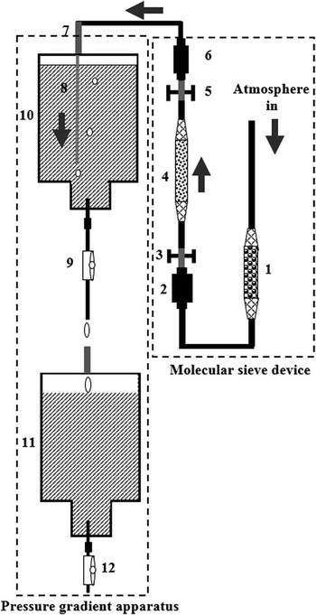
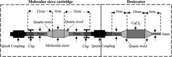
The CO2 sampling device is composed of two parts (Figure 1): (1) a molecular sieve device and (2) pressure gradient apparatus. The molecular sieve device includes a molecular sieve cartridge (MSC), which is a modification of the one previously described by Hardie et al. (Reference Hardie, Garnett, Fallick, Rowland and Ostle2005) and Garnett et al. (Reference Garnett, Hartley, Hopkins, Sommerkorn and Wookey2009), and desiccator as shown in Figure 2.
Schematic illustration of the CO2 sampling device: (1) desiccator; (2) quick coupling; (3) clip; (4) molecular sieve cartridge (MSC); (5) clip, (6) quick coupling; (7) glass tube; (8) silicone tubing; (9) flow regulator; (10) glass bottle 1; (11) glass bottle 2; (12) flow regulator.

Schematic diagram of the molecular sieve device

The MSC was made in a quartz tube and the center of cartridge [12 mm outside diameter (OD), 60 mm length] was filled with 5 g of 13X molecular sieve (1/16″ pellets, Pingxiang Naike Chemical Industry Equipment Packing Co., Ltd, China), and secured with quartz wool at the ends. Typically, 100 g of the 13X sieve has the capacity to store ~0.5 g of CO2 (Giacobbe Reference Giacobbe1991). In practice, more sieve is selected to ensure successful collections; thus, 5 g were used in this paper. Both ends of each cartridge (9 mm OD, 120 mm length) were sealed by two auto-shutoff Quick Couplings (Colder Products Company, USA) attached via short lengths of tubing (Tygon, Fisher, UK). When not mated to other couplings, the couplings on the MSC automatically sealed and a clip was placed across the tubing to form an additional seal. During sampling, one end of the MSC was attached with the quick coupling placed on the pump of the CO2 sampling device, and the other end of the MSC was attached with the desiccator constructed using a glass tube (18 mm OD, 100 mm length) filled with CaCl2 (AR, 1–2 mm pellets, Beijing Chemical Industry Co., Ltd, China), as shown in Figure 2.
The pressure gradient apparatus consisted of an 8000-mL custom-made glass bottle with a water flow regulator at the bottleneck, with a 9-mm-OD, 60-mm-long glass tube attached to the bottle (Figure 1). This device is designed to actively absorb CO2 from the atmosphere. The water pressure induces a gradient between the inside and outside of the bottle, driven by the water flowing out of the glass bottle, drop by drop. Atmospheric CO2 is actively absorbed onto the molecular sieve. The flow rate can be controlled by a regulator to meet a targeted sampling duration (e.g. hours, days, or weeks). In addition, the dripping water can be collected in a separate glass bottle for reuse as shown in Figure 1.
Before sampling, we ensure that an adequate pressure gradient is achieved using the following steps (with numbered references to Figure 1):
-
1. Place an 8000-mL glass bottle on the support, close the flow regulator (9), and insert a 5-mm-OD, 200-mm-long silicon pipe (8), which extends from an upper glass tube (7) to the bottom of the first glass bottle (10).
-
2. Link the MSC (4) with the glass tube (7) using the quick coupling (6), and connect the quick coupling (2) with one side of the desiccator tube (1), then open clips (3) and (5).
-
3. Seal the air intake of the desiccator tube (1), and maximize the flow regulator (9) to initiate water flow. Wait about 30 s. When the dripping stops, a pressure gradient has been achieved.
-
4. Open the air-intake of the desiccator tube (1), adjust the flow regulator to the desired rate (9), and begin sampling.
-
5. If the water in the glass bottle (10) runs out, replace the glass bottle (11) to continue sampling, and repeat the procedure above until meeting the targeted sampling duration.
-
6. When finished, remove the molecular sieve device (4), and insert it into a furnace to liberate CO2.
Molecular Sieve Cartridge Activation and Desorption
We designed a 60-mm-OD×250-mm-long muffle tube furnace, with a zone of uniform temperature of about 150 mm. In the center of this tube furnace, there is a zone of uniform temperature that extends to about 2.5 times the diameter of the tube measured from the outside of the furnace (Hardie et al. Reference Hardie, Garnett, Fallick, Rowland and Ostle2005). We introduced a quartz cartridge with molecular sieve (MSC), which is 12 mm OD, 60 mm length. The length of uniform temperature within the muffle furnace can assure complete sample recovery when desorbing the molecular sieve.
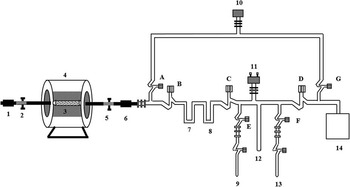
The MSC should be activated completely before sampling to ensure that it is free of contamination. Prior to inserting the MSC into a tube furnace, one side was connected to a source of high-purity N2. The MSC was then inserted into a tube muffle furnace and heated to 550°C, and high-purity (99.999%) N2 was passed through the sieve at a rate of 180 mL/min for at least 20 min (Figure 3). The MSC was allowed to cool to <30°C and filled with high-purity N2 gas at a pressure slightly above atmospheric (~1100 mbar). We also noted a minor amount of hysteresis that cannot absorb CO2 completely in the molecular sieves on their first use. The fresh molecular sieve was first purged of all gases and then flushed with CO2 in an air stream and repurged prior to sampling (Hardie et al. Reference Hardie, Garnett, Fallick, Rowland and Ostle2005).
Schematic illustration of the MSC desorption: (1) quick coupling; (2) clip; (3) MSC; (4) tube furnace; (5) clip; (6) quick coupling; (7) cold trap 1; (8) cold trap 2; (9) gas collection unit; (10) vacuum gauge; (11) pressure transducer; (12) cold finger; (13) gas collection unit; (14) vacuum pump.

The following steps were followed to desorb the CO2 from the sample cartridges after sampling (with reference to Figure 3). The MSC was inserted into a tube furnace and attached to a vacuum with a quick coupling and evacuated to less than 10–2 Torr. The connections leading up to the cartridge were then evacuated. Cold trap 1 (–76°C) was cooled with a liquid nitrogen and alcohol mixture for removing H2O and other gases, while cold trap 2 (–196°C) was cooled with liquid nitrogen for collecting CO2 gas. The vacuum system was then isolated and the furnace temperature was raised to 550°C. CO2 was collected at this temperature under a static vacuum for 20 min. Non-condensable gases were pumped away after a vacuum of 10–2 Torr was achieved in the system. The CO2 was transferred to a calibrated volume between valves C and D, and the pressure of the gas was measured using a pressure transducer (Type 660, MKS, USA) to determine the amount of CO2 collected. A portion of the CO2 was reduced to graphite with a Zn/Fe catalytic reduction (Slota et al. Reference Slota, Jull and Linick1987; Jull Reference Jull2007) for the AMS analysis. The AMS measurements were performed with a 3MV tandem accelerator at the Xi’an AMS Centre, Xi’an, China (Zhou et al. Reference Zhou, Zhao, Lu, Liu, Wu, Peng, Zhao and Huang2006). A second portion of the CO2 sample were measured for 13C by a Thermo Finnigan DELTA plus XL isotope ratio mass spectrometer in the Institute of Earth Environment, Chinese Academy of Sciences (IEECAS).
DISCUSSION
Test of Laboratory Methods
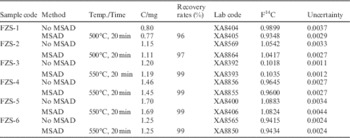
A total of six CO2 gas samples were used to test the recovery rate onto the molecular sieve. Each gas sample was divided into two equal C mass portions. One portion of the CO2 was directly converted into graphite for 14C measurement, while another portion of the CO2 was used for molecular sieve absorption and desorption (MSAD), described by our methods above, and the recovered CO2 was converted into graphite for AMS 14C analysis. AMS results are expressed as fraction of modern carbon (F) values, defined following Donahue et al. (Reference Donahue, Linick and Jull1990).
We observed a recovery rate of 96–97% for the customized tube furnace at a temperature of 500°C and collection time of 20 min, and repeated F14C values were beyond errors at the 2σ level. Sample recovery was improved (to 99%) by increasing the desorption temperature to 550°C (Table 1). These parameters also gave good reproducibility at the 2σ level, so these conditions were adopted for routine sampling.
Results of mass and F 14C without MSAD and with MSAD

Comparison with the Phosphoric Acid Solution Displacement Method
We collected atmospheric samples from the same locality at the same time for a comparative study. All of the 13C values are reported using the delta notation with 13C/12C variations relative to the international standard Vienna Pee Dee Belemnite (VPDB). The 14C results are reported as fraction modern carbon (F) values (Donahue et al. Reference Donahue, Linick and Jull1990).
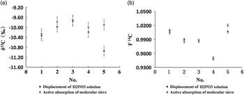
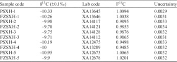
Figure 4 and Table 2 show good overall reproducibility between the two methods at the 2σ uncertainty level. There is evidence for a small systematic difference in sample 5, both for 13C (~1‰) and 14C (~1%); however, the overall agreement is very consistent, so we consider both methods viable for sampling.
Comparison between the phosphoric acid solution displacement method and active absorption on a molecular sieve: (a) δ13C results of the two methods, (b) F14C results of the two methods.

δ13C and F 14C results of the two methods.

Note: PSXH represents the displacement of H3PO4 solution method, and FZSXH represents active absorption of molecular sieve by pressure gradient from the water process.
APPLICATION EXAMPLES
Atmospheric CO2 Sample Collection
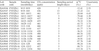
We collected atmospheric samples over about a 3-month period (15 September to 16 December 2013). Samples of atmospheric CO2 were taken from the roof of the Xi’an AMS building. Xi’an’s elevation is 440 m above sea level. The results are given in Table 3.
Atmospheric CO2Δ14C results for September 15 to December 16.

When the flow rate was less than 3 mL/min, as the water volume in the glass bottle gradually decreased, it stopped dripping. When the flow rate was more than 3 mL/min, it changed slightly as the water volume decreased, we were able to keep the flow rate as 3 mL/min by using a water flow regulator. The flow regulator was adjusted to around 3 mL/min, indicating water in an 8000-mL glass bottle will run out within 2 days. After 2 days, we renewed the glass bottle to continue sampling until we meet the targeted sampling duration. 14C results are reported as Δ14C values (Stuiver and Polach Reference Stuiver and Polach1977), see Table 3.
CO2ff values were calculated with the following equation (Levin et al. Reference Levin, Kromer, Schmidt and Sartorius2003; Kuc et al. Reference Kuc, Rozanski, Zimnoch, Necki, Chmura and Jelen2007; Zhou et al. Reference Zhou, Wu, Huo, Xiong, Cheng, Lu and Niu2014):
 $$CO_{{2ff}} {\rm {\equals}}{{CO_{{2obs}} (\rDelta _{{obs}} {\minus}\rDelta _{{bg}} )} \over {\rDelta _{{ff}} {\minus}\rDelta _{{bg}} }}$$
where Δ ff is –1000‰, Δ obs is the Δ14C of the air samples, and Δ bg is the Δ14C of the atmospheric background site.
For air samples, CO2obs was derived by averaging continuously measured CO2 data using a Picarro G2131-i CO2 Carbon Stable Isotope Analyzer. The CO2 mole fraction was measured about once a second at the 14CO2 sampling site of the Institute of Earth Environment, Chinese Academy of Sciences (IEECAS), with a precision of 0.1 ppm.
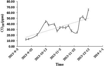
Figure 5 shows that fossil fuel emissions were on the rise from September to December, with an average increase of ~0.4 ppm per day. We attribute this to the enhancement of coal burning for heating. The available 14C measurement precision decreases with decreasing sample size. Our collection method has an average absorption rate of 1.0 mg C/day, much greater than that of passive absorption rates (e.g. 0.044 to 0.065 mg C/day, Walker et al. Reference Walker, Xu, Fahrni, Lupascu and Czimczik2015). Over a 5-day integration period, our method is able to capture sufficient carbon for high-precision 14C AMS, necessary for fossil-fuel apportionment studies.
Trend of fossil fuel CO2 mole fraction with time

Soil Respiration CO2 Collection
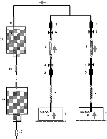
Two MSCs were used for collecting respired CO2 from a disturbed soil and a grassland for 6 and 12 hr, respectively. When the flow rate is more than 20 mL/min, there is no obvious change as the water volume decreases. The flow regulator was then adjusted to around 20 mL/min. When the water in the glass bottle ran out, we renewed the glass bottle to continue sampling until 12 hr had passed.
First, we pumped out the air from 8000-mL glass chamber for 10 min, then stopped pumping, waited for 1 hr so that CO2 from soil respiration would fill in a glass chamber, and we then connected the chamber to the inlet of the CO2 collection (Figure 6).
Schematic illustration of the soil respiration CO2 collection: (1) glass chamber; (2) desiccator; (3) quick coupling; (4) clip; (5) MSC; (6) clip; (7) quick coupling; (8) glass tube; (9) silicone tube; (10) flow regulator; (11) glass bottle 1; (12) glass bottle 2.

The results in Table 4 show that the F 14C for the disturbed soil and grassland had no statistical difference found for each site for the 6-hr and 12-hr integration time. Therefore, the method seems very suitable for taking soil gas samples.
F14C results collected from different soil types.

CONCLUSION
Our method makes use of a pressure gradient produced between the inside and outside of a bottle while water is a flowing through it, one drop at a time. This allows us to continually absorb CO2 into a molecular sieve to collect a sufficient quantity for high-precision AMS 14C measurements. We describe a customized tube muffle furnace used to desorb the CO2 in the laboratory. We find that a desorption temperature of 550°C for at least 20 min is optimal, yielding recovery rates above 99% with good reproducibility. A comparison study of our method with our phosphoric acid solution displacement method gave comparable 13C and 14C results, and as the molecular sieve technique avoids the use of handling dangerous acid in the field, we see this as a distinct advantage. For atmospheric CO2 sampling, the average absorption rate was 1.0 mg C/day by this method, which allows for high-precision AMS 14C measurements. For soil CO2 respiration sampling, our results showed that the F14C of a disturbed soil and a grassland showed no statistical difference for each site at the 6-hr and 12-hr integration time. The method thus seems very suitable for taking soil gas samples.
ACKNOWLEDGMENTS
The authors would like to express sincere thanks to the staff of the Xi’an AMS Center for their technical support. Special thanks go to Prof Weijian Zhou for her enlightening suggestions on experimental improvement and Prof G S Burr for English improvement and his valuable suggestions on the previous drafts of this manuscript. This work was jointly supported by grants from National Basic Research Program of China (2013CB955900), Natural Science Foundation of China, and The Ministry of Science and Technology Special Science and Technology Foundation (2015FY110800).