1 Introduction
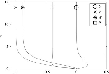
The set-up considered here is a rotating disk in an incompressible fluid. The rotating-disk flow is also known as the von Kármán flow (von Kármán Reference von Kármán1921). The scaled velocity profiles of figure 1 show an exact solution to the incompressible Navier–Stokes equations. The simplicity of the von Kármán flow has made it suitable to serve as a model for other three-dimensional boundary layers as suggested for example by Gregory, Stuart & Walker (Reference Gregory, Stuart and Walker1955).
The von Kármán velocity profiles in the rotating reference frame for the flow over an infinite rotating disk.
 $U$
is the radial velocity component,
 $V$
is the azimuthal velocity component,
 $W$
is the vertical velocity component and
 $P$
is the pressure. The pressure is normalized to zero at the wall.

This flow case has been of interest for stability and transition research for some time, and the finding of Lingwood (Reference Lingwood1995) that the boundary layer becomes (linearly) absolutely unstable above a threshold Reynolds number was of particular significance. Prior to this, extensive theoretical investigations had been made, e.g. Mack (Reference Mack1985), Malik (Reference Malik1986), and the two main convectively unstable modes together with a family of damped modes had been found. Lingwood (Reference Lingwood1995) indicated the significance of one of the damped modes by showing that it exhibited a pinch point with one of the unstable modes where the group velocity was zero, giving rise to the absolute instability. After this discovery, more theoretical research has been undertaken, trying to translate this local behaviour to a global frame, e.g. Pier (Reference Pier2003, Reference Pier2007), mainly looking for signs that this absolute instability is responsible for the onset of transition to turbulence observed in experiments. Experimental studies of the disk flow can also be divided into those performed prior to Lingwood (Reference Lingwood1995) and those after. Prior to 1995, most studies were focussed on the stationary vortices, e.g. Wilkinson & Malik (Reference Wilkinson and Malik1985), whereas Lingwood (Reference Lingwood1996) explored the possibility of a global instability in the flow field resulting from the absolute instability, with follow-up experiments in this vein by e.g. Othman & Corke (Reference Othman and Corke2006), Siddiqui et al. (Reference Siddiqui, Mukund, Scott and Pier2013), Imayama, Alfredsson & Lingwood (Reference Imayama, Alfredsson and Lingwood2014). Lingwood (Reference Lingwood1995) found that the absolute instability had a critical Reynolds number (
 $R_{cl}$
) of 507 (first given as 510 and then corrected in Lingwood Reference Lingwood1997). The Reynolds number for the rotating-disk flow is here defined as
 $$\begin{eqnarray}\displaystyle R=r^{\ast }\sqrt{\frac{\unicode[STIX]{x1D6FA}^{\ast }}{\unicode[STIX]{x1D708}}}=r, & & \displaystyle\end{eqnarray}$$
where
 $^{\ast }$
refers to a dimensional quantity,
 $r^{\ast }$
is the radial position on the disk and
 $\sqrt{\unicode[STIX]{x1D708}/\unicode[STIX]{x1D6FA}^{\ast }}$
is the length scale used, where
 $\unicode[STIX]{x1D708}$
is the (dimensional) kinematic viscosity of the fluid and
 $\unicode[STIX]{x1D6FA}^{\ast }$
is the angular velocity of the disk.
In 2003, the first (known to the authors) direct numerical simulation (DNS) of the linearized Navier–Stokes equations was reported (Davies & Carpenter Reference Davies and Carpenter2003), computing both the local and global flow behaviours. The local behaviour showed exactly what was expected from theory: an absolute instability, whereas the global behaviour showed no sign of one. Pier (Reference Pier2003, Reference Pier2007) therefore based his nonlinear theoretical work on the underlying assumption that the flow was linearly globally stable. Further investigations were also made by Davies, Thomas & Carpenter (Reference Davies, Thomas and Carpenter2007) to investigate effects of the inhomogeneous base flow, when
 $R$
varies with
 $r$
, of the infinite disk. They managed to mimic the stable behaviour of the disk boundary layer through a Ginzburg–Landau model if the temporal frequency varied linearly with radius. This ‘detuning’ effect created a spatial variation in the temporal growth rate and thus stabilized the flow. The results of Davies & Carpenter (Reference Davies and Carpenter2003) also led to further numerical simulations to determine whether their finding of linear global stability was also applicable to a finite disk in contrast to the infinite disk assumed in their simulations. Healey (Reference Healey2010) investigated this flow case using a linearized Ginzburg–Landau model and Appelquist et al. (Reference Appelquist, Schlatter, Alfredsson and Lingwood2015a
) considered DNS of the flow over a finite disk.
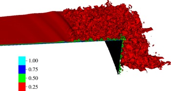
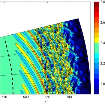
In the previous work of Appelquist et al. (Reference Appelquist, Schlatter, Alfredsson and Lingwood2015a ,Reference Appelquist, Schlatter, Alfredsson and Lingwood b ), a nonlinear simulation was included both to justify the use of a sponge region in the linear simulations, modelling the effect of the turbulent outer annulus on an inner flow region, and also to analyse the nonlinear behaviour. A linear global mode induced by the turbulence was found and has been shown to maintain the turbulence within the domain, as a global instability would. In this paper, this nonlinear behaviour is further analysed and, in addition, two simulations where the actual edge of the disk is included are discussed: one where the disk is assumed to be infinitely thin; and a case with a physically realistic edge to allow for comparisons with experiments. Figure 2 is a three-dimensional visualization from the latter simulation that shows isosurfaces of the azimuthal velocity normalized by the local disk speed and, in particular, a nonlinear front can be seen. It is precisely these fronts found in the DNS that will be analysed and characterized in the present paper.
Isosurfaces pertaining to case NL03 showing the azimuthal velocity normalized by the disk speed (
 $V_{N}$
) in the laboratory frame of reference at
 $T=6$
.

The nonlinear theory studied by Pier (Reference Pier2003, Reference Pier2007) predicted a so-called ‘elephant’ global mode in the rotating-disk boundary layer. These results are based on the previous theoretical work on steep nonlinear global modes where Pier et al. (Reference Pier, Huerre, Chomaz and Couairon1998) showed that a frequency selection takes place at a position where an upstream (
 $-$
) branch is linked to a downstream (
 $+$
) branch. For a steep global mode, the position where a linear upstream branch
 $k^{l-}$
and a nonlinear downstream branch
 $k^{nl+}$
meet acts as a frequency generator for the entire flow. This position separates the convectively unstable region from the absolutely unstable region (
 $R_{cl}$
) acting as a local oscillator inducing both the upstream (
 $-$
) branch and the downstream (
 $+$
) branch. The
 $k^{l-}$
branch then lies completely in the convectively unstable region whereas the
 $k^{nl+}$
branch lies in the absolutely unstable region. The steep global mode just described was first referred to as an ‘elephant mode’ in Pier & Huerre (Reference Pier and Huerre2001). They showed that the von Kármán vortex street is of elephant-mode type and that the elephant frequency-selection criterion agrees with the frequency of the vortex shedding. The selection criterion is given by the local absolute instability. Since the absolute instability, which is a local property, selects an elephant mode at transition whenever an absolutely unstable region is present, the absolute instability is a necessary and sufficient condition for the existence of self-sustained nonlinear structures. The conclusion of Pier & Huerre (Reference Pier and Huerre2001) was that a nonlinear global instability takes place as soon as a local absolute instability arises at some point in the flow. The nonlinear elephant global mode is thus governed by local linear properties. Two kinds of such nonlinear elephant modes have been described in the literature, i.e. pulled and pushed elephant modes, see Chomaz (Reference Chomaz2004). The kind described above is a pulled front, which would be seen as a stationary front located at
 $R_{cl}$
, which is itself absolutely unstable to secondary instabilities. Such a front has been found in the DNS by Viaud, Serre & Chomaz (Reference Viaud, Serre and Chomaz2008, Reference Viaud, Serre and Chomaz2011) in an open rotating cavity. They found that their flow was linearly globally stable and nonlinearly globally unstable, leading to a subcritical global instability. At
 $R_{cl}$
, a sharp front grew and downstream a saturated nonlinear spiral mode was fixed by properties from linear theory. This downstream mode also contained an elephant mode and a direct transition to turbulence was given through an elephant-mode cascade where an absolute secondary instability gives rise to a secondary elephant mode. The structure of the flow field in figure 3(b) in Viaud et al. (Reference Viaud, Serre and Chomaz2011) is similar to that of the disk.
The second type of nonlinear elephant global mode, the pushed front, has a propagation speed determined by the nonlinear behaviour downstream. This contrasts with the pulled front where the front propagation speed is determined by the linear global mode. For either type of elephant mode, the linear upstream branch (
 $k^{l-}$
) meets the nonlinear downstream branch (
 $k^{nl+}$
) at a certain position in space. For our simulations this position will be estimated and called
 $r_{end}$
, consistent with previous presentation of results in Appelquist et al. (Reference Appelquist, Schlatter, Alfredsson and Lingwood2015a
,Reference Appelquist, Schlatter, Alfredsson and Lingwood
b
). This definition of
 $r_{end}$
indicates the end of the linear region. For
 $r>r_{end}$
the flow will have entered the nonlinear region and
 $r_{end}$
thus separates the linear and nonlinear regions. In experiments, Imayama, Alfredsson & Lingwood (Reference Imayama, Alfredsson and Lingwood2013) defined the transitional Reynolds number (also including Imayama, Alfredsson & Lingwood (Reference Imayama, Alfredsson and Lingwood2012, Reference Imayama, Alfredsson and Lingwood2014, Reference Imayama, Alfredsson and Lingwood2016)) from their power spectra where the first harmonic of the stationary vortices reached an amplitude of
 $10^{-6}$
. Using this threshold for the onset of nonlinearity in our simulations, it will be shown that the first harmonics of the travelling disturbances reach the same amplitude in our corresponding spectra at our position
 $r_{end}$
. Furthermore, Imayama et al. (Reference Imayama, Alfredsson and Lingwood2013) summarize the transitional Reynolds numbers of various experiments in their table 1 showing that a wide range of definitions have been used by different authors. In their table 3, they have translated a few of these: Kobayashi, Kohama & Takamadate (Reference Kobayashi, Kohama and Takamadate1980), Malik, Wilkinson & Orszag (Reference Malik, Wilkinson and Orszag1981), Wilkinson & Malik (Reference Wilkinson and Malik1985), Lingwood (Reference Lingwood1996) and Othman & Corke (Reference Othman and Corke2006) to their own definition of onset of nonlinearity for comparison, on which they base their resulting transitional Reynolds number (
 $R=510{-}520$
), including their own data. Also Viaud et al. (Reference Viaud, Serre and Chomaz2008, Reference Viaud, Serre and Chomaz2011) use a corresponding position to our
 $r_{end}$
for their primary front found in simulations of a rotating cavity. The position of their primary front is shown to be followed by a saturated wave, and corresponds to
 $R_{cl}$
for the rotating cavity.
Studies of the proximity of the edge to the transition Reynolds number have also been reported in the literature. Healey (Reference Healey2010) also investigated the effect of nonlinearity by adding a term to his Ginzburg–Landau model and found a (supercritical) nonlinear front appearing at the onset of absolute instability when the disk edge was far from the front itself. However, he found that when the disk edge approached
 $R_{cl}$
the onset of absolute instability moves radially outwards, i.e. the proximity of the edge stabilized the flow. Experiments by Imayama et al. (Reference Imayama, Alfredsson and Lingwood2013) showed no obvious variation in the transition Reynolds number when
 $R_{cl}$
was close to the edge while Pier (Reference Pier2013) found in his experiments that the edge of the disk acted as a strong source of fluctuations. Having a physical edge included in the DNS gives the opportunity to investigate its effect on the boundary layer and check whether the perturbations from the edge enter into the rotating-disk boundary layer. We do not, however, aim here to examine how the proximity of the edge affects
 $R_{cl}$
, and leave this for future numerical studies.
This paper is organized as follows. In § 2 the set-up of the simulations is described. Results are presented in § 3 including a discussion, and finally § 4 provides a summary and conclusions.
2 Method
The simulations were performed with the massively parallel code Nek5000 (Fischer, Lottes & Kerkemeier Reference Fischer, Lottes and Kerkemeier2012) using a spectral element method (SEM). The code is the same as used in Appelquist et al. (Reference Appelquist, Schlatter, Alfredsson and Lingwood2015a
) however a minor correction is given here; namely that the
 $P_{N}$
–
 $P_{N-2}$
method is used in both papers. This describes the spatial discretization where the pressure is only defined on the Gauss–Legendre points, in contrast to the velocity fields that are defined on Gauss–Lobatto–Legendre points. The reason for this is to remove spurious pressure modes. Again Legendre polynomials of order 7 are used. SEM was introduced by Patera (Reference Patera1984) and combines the geometrical flexibility of finite element methods with the accuracy of spectral methods. The temporal discretization scheme in Nek5000 is based upon operator splitting, where the nonlinear convective terms are treated explicitly via an extrapolation scheme (EXT) and the viscous and divergence operators are treated implicitly. The implicit scheme is based on the backward differential formula (BDF). Equation (15) in Karniadakis, Israeli & Orszag (Reference Karniadakis, Israeli and Orszag1991) corresponds to the operative scheme BDFk/EXTk, where in Nek5000 orders of
 $k=1,2,3$
are possible.
2.1 Governing equations
The full Navier–Stokes equations are advanced in time within the Nek5000 code
 $$\begin{eqnarray}\displaystyle \frac{\unicode[STIX]{x2202}\boldsymbol{U}_{\boldsymbol{x}}}{\unicode[STIX]{x2202}t}+\boldsymbol{U}_{\boldsymbol{x}}\boldsymbol{\cdot }\unicode[STIX]{x1D735}\boldsymbol{U}_{\boldsymbol{x}}=-\unicode[STIX]{x1D735}p+\frac{1}{R_{N}}\unicode[STIX]{x1D6FB}^{2}\boldsymbol{U}_{\boldsymbol{x}}+\boldsymbol{f}_{\boldsymbol{x}} & & \displaystyle\end{eqnarray}$$
together with the continuity equation
 $$\begin{eqnarray}\displaystyle \unicode[STIX]{x1D735}\boldsymbol{\cdot }\boldsymbol{U}_{\boldsymbol{x}}=0, & & \displaystyle\end{eqnarray}$$
where
 $\boldsymbol{U}_{\boldsymbol{x}}=(U_{x},U_{y},W)$
are the velocities in Cartesian coordinates,
 $p$
is the pressure and
 $\boldsymbol{f}_{\boldsymbol{x}}$
is a forcing term used in connection with the initial disturbance, fictional forces (if included) and sponge regions used together with the radial boundary conditions. The nonlinearity in the advection can be turned off so that the code is run in only a linear fashion, which was the approach taken in Appelquist et al. (Reference Appelquist, Schlatter, Alfredsson and Lingwood2015a
). The flow field for the linear code is divided into a base flow and an additional perturbation field. For the velocities in cylindrical coordinates the notation
 $\boldsymbol{U}=(U,V,W)$
is used. The scaling of these velocities and the additional pressure in the global scale are
 $U=U^{\ast }/r^{\ast }\unicode[STIX]{x1D6FA}^{\ast }$
,
 $V=V^{\ast }/r^{\ast }\unicode[STIX]{x1D6FA}^{\ast }$
,
 $W=W^{\ast }/(\unicode[STIX]{x1D708}\unicode[STIX]{x1D6FA}^{\ast })^{1/2}$
and
 $P=P^{\ast }/\unicode[STIX]{x1D70C}\unicode[STIX]{x1D708}\unicode[STIX]{x1D6FA}^{\ast }$
, where
 $\unicode[STIX]{x1D70C}$
is the dimensional density. The time scale within the simulations is such that
 $t$
corresponds to the number of radians through which the disk has rotated. The number of full rotations is measured by
 $T=t/(2\unicode[STIX]{x03C0})$
. The parameter
 $R_{N}$
in (2.1) refers to the numerical Reynolds number used in the simulations directly related to the size of the numerical domain. For our simulations this was chosen to be 1, giving the desired relationship
 $R=r$
. An extensive description of this scaling can be found in Appelquist (Reference Appelquist2014). There, a description of the accuracy of the laminar flow can also be found to be of the order of
 $10^{-8}-10^{-12}$
when using an efficient spectral interpolation routine to extract equidistant points from the SEM mesh.
Summary of the spectral element mesh for the linear simulations in terms of size of the domain [min max], number of spectral elements (
 $N_{r}$
,
 $N_{\unicode[STIX]{x1D703}}$
and
 $N_{z}$
in the
 $r$
,
 $\unicode[STIX]{x1D703}$
and
 $z$
directions, respectively) and resolution of the spectral elements in the radial, azimuthal and wall-normal directions.

2.2 Mesh and simulations
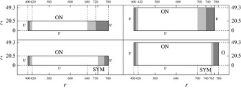
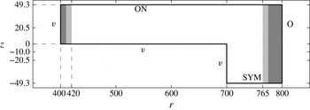
The domain sizes of the simulations in the
 $r$
–
 $z$
plane are shown in figures 3 and 4. Two linear simulations, L01 and L02, have been performed with a total of 21 120 spectral elements each. Their mesh characteristics are summarized in table 1, and with a typical linear disturbance with a radial wavelength of 4.8 (corresponding to a disturbance with
 $\unicode[STIX]{x1D6FC}_{r}=0.2088$
), an azimuthal wavelength of
 $2\unicode[STIX]{x03C0}/68$
and a boundary layer thickness for the laminar profile where
 $V=0.05$
of 3.60, this mesh is well resolved. These simulations were run for a time of, respectively,
 $T=3.25$
and
 $T=2.5$
. The difference between these two linear simulations is the boundary conditions used. The L01 case uses a sponge region corresponding exactly to case r04 in Appelquist et al. (Reference Appelquist, Schlatter, Alfredsson and Lingwood2015a
). Case L02 is also mentioned in Appelquist et al. (Reference Appelquist, Schlatter, Alfredsson and Lingwood2015a
), and turns out to be linearly stable although the data are further analysed in this paper in relation to the corresponding nonlinear simulation NL02. Both L02 and NL02 include a disk edge with a symmetry boundary condition (SYM), where the domain is mirrored in the
 $z$
direction corresponding to an infinitely thin disk. The simulation NL03 also includes a symmetry boundary condition but with a finite-thickness edge included in the simulation. The set-up of NL03 can easily be related to the physical disks used in experiments. The thickness of the disk in NL03 corresponds to almost 40 mm if mirrored in the vertical plane, for a disk with rotational speed of 1000 rotations per minute in air at
 $20\,^{\circ }\text{C}$
(
 $\unicode[STIX]{x1D708}=1.5\times 10^{-5}~\text{m}^{2}~\text{s}^{-1}$
). The experimental radius would then correspond to
 $265$
mm if the edge Reynolds number is 700. The spectral element mesh for the nonlinear simulation NL01 is presented in table 2. Simulations NL02 and NL03 have spectral elements clustered close to the edge of the disk (
 $r=700$
) in order to resolve the sudden change in geometry or boundary condition. Table 2 can then be seen as a reference of minimum resolution of the spectral elements. The number of spectral elements for the three nonlinear simulations conducted, NL01, NL02 and NL03 are 183 551, 186 434 and 221 991, respectively. All nonlinear simulations were run to a time of
 $T=6$
. A resolution check was undertaken for case NL02 for another half rotation where the polynomial order was increased from 7 to 9 and no difference was seen. Simulations L01, L02, NL02 and NL03 were performed in the laboratory frame of reference, whereas NL01 was run in the rotating frame of reference. The reason for this was to keep the velocity small for the flow beyond the edge of the disk, where in the laboratory frame of reference both NL02 and NL03 have velocities decaying to zero. Since the edge was not included in NL01 this was preferably run in the rotating frame of reference for a more direct comparison to theory, which is performed in this reference frame. The linear simulations L01 and L02, however, appear in Appelquist et al. (Reference Appelquist, Schlatter, Alfredsson and Lingwood2015a
) where all simulations were performed in the laboratory frame of reference.
The extent of the domains in
 $r$
–
 $z$
of cases L01 (top left), NL01 (top right), L02 (bottom left) and NL02 (bottom right). The boundary conditions are marked ‘
 $v$
’. ‘O’, ‘ON’ and ‘SYM’ stand for Dirichlet, homogeneous Neumann outflow, a mixture of both Dirichlet and homogeneous Neumann and finally a symmetry condition. Formal descriptions of the conditions are given in the text. Also a sponge region is seen in grey scale and is explained in the text.

Similar to figure 3, but for case NL03.

Summary of the spectral element mesh for the nonlinear simulation NL01 (see table 3), again, in terms of size of the domain [min max], number of spectral elements (
 $N_{r}$
,
 $N_{\unicode[STIX]{x1D703}}$
and
 $N_{z}$
in the
 $r$
,
 $\unicode[STIX]{x1D703}$
and
 $z$
directions, respectively) and resolution of the spectral elements in the radial, azimuthal and wall-normal directions.

The included angle of the domain considered is
 $2\unicode[STIX]{x03C0}/68$
where 68 is chosen since this is the azimuthal wavenumber of the onset of local absolute instability according to linear theory. In the wall-normal direction the elements are stretched according to
 $$\begin{eqnarray}\displaystyle z_{n}=\mathop{\sum }_{i=1}^{n}\unicode[STIX]{x0394}zs^{i-1}, & & \displaystyle\end{eqnarray}$$
where
 $s$
is the stretching factor,
 $z_{n}$
is the coordinate at position
 $n$
above the wall and
 $z_{1}=\unicode[STIX]{x0394}z$
is the height of the spectral element closest to the wall. These parameters are also seen in tables 1 and 2. An advantage of defining the coordinate system in such a way is the equivalence to the geometric sum
 $$\begin{eqnarray}\displaystyle z_{n}=\frac{s^{n}-1}{s-1}\unicode[STIX]{x0394}z & & \displaystyle\end{eqnarray}$$
giving a direct relationship between a mesh coordinate and an array position in our code.
2.3 Boundary conditions
There are different boundary conditions seen in figures 3 and 4 in relation to the simulations. A formulation of the already mentioned symmetric boundary condition would be an impermeable plane where
 $W=0$
, and
 $\unicode[STIX]{x2202}U/\unicode[STIX]{x2202}z=0$
and
 $\unicode[STIX]{x2202}V/\unicode[STIX]{x2202}z=0$
. The Dirichlet boundary condition is denoted with ‘
 $v$
’ and is always set to the von Kármán similarity solution. A homogeneous Neumann outflow boundary condition is denoted with ‘O’, and ‘ON’ combines both
 $v$
and O to set the in-plane velocities but leaves the normal velocity to be stress free:
 $\unicode[STIX]{x2202}W/\unicode[STIX]{x2202}z=p$
. A segmentation of the domain to only
 $2\unicode[STIX]{x03C0}/68$
radians was made possible through cyclic boundary conditions in the azimuthal direction, which are essentially periodic boundary conditions but involve an appropriate rotation of the velocities across the boundary.
The grey shaded areas in figures 3 and 4 are sponge regions also described in Appelquist et al. (Reference Appelquist, Schlatter, Alfredsson and Lingwood2015a
) applying a volume force to the velocity field such that the solution relaxes to the von Kármán laminar flow field. Figure 2 therein shows
 $\unicode[STIX]{x1D706}(r)$
used in the forcing function
 $$\begin{eqnarray}\displaystyle \boldsymbol{f}=-\unicode[STIX]{x1D706}(r)\boldsymbol{u}, & & \displaystyle\end{eqnarray}$$
where
 $\boldsymbol{f}$
in cylindrical coordinates is converted to
 $\boldsymbol{f}_{\boldsymbol{x}}$
in Cartesian coordinates before entering (2.1) in our simulations. The sponge function
 $\unicode[STIX]{x1D706}$
is described by
 $$\begin{eqnarray}\displaystyle \unicode[STIX]{x1D706}(r)=\unicode[STIX]{x1D706}_{max}\left[S\left(\frac{r-r_{start}}{\unicode[STIX]{x1D6E5}_{rise}}\right)\right], & & \displaystyle\end{eqnarray}$$
where the maximum strength of the damping is
 $\unicode[STIX]{x1D706}_{max}$
, the radial position where the sponge region starts is
 $r_{start}$
and
 $\unicode[STIX]{x1D6E5}_{rise}$
corresponds to the rise distance of the damping function. The smooth step function
 $S$
, using
 $x$
as the argument, is
 $$\begin{eqnarray}\displaystyle S(x)=\left\{\begin{array}{@{}ll@{}}0,\quad & x\leqslant 0,\\ 1/(1+\text{e}^{1/(x-1)+1/x}),\quad & 0<x<1,\\ 1,\quad & x\geqslant 1.\end{array}\right. & & \displaystyle\end{eqnarray}$$
The corresponding
 $\unicode[STIX]{x1D6E5}_{rise}$
parameters describe a smooth increase of the force and are shown as light grey shaded areas and the areas where
 $\unicode[STIX]{x1D706}_{max}$
is achieved are illustrated in dark grey in our figures 3 and 4. The
 $\unicode[STIX]{x1D706}_{max}$
values were [28, 10, 18, 8, 8] for simulations [L01, NL01, L02, NL02, NL03]. For the two cases with a sponge prior to the ‘O’ condition, only
 $V$
and
 $W$
were forced back to the similarity solution to reduce the vorticity in the fields before the outflow. A sponge was also used for the inflow region where the function (2.6) was tuned to damp in the opposite direction. Then
 $r_{start}=420$
,
 $\unicode[STIX]{x1D6E5}_{rise}=10$
was used in the negative
 $r$
-direction, and
 $\unicode[STIX]{x1D706}_{max}=0.8$
for all simulations, which is the same as in Appelquist et al. (Reference Appelquist, Schlatter, Alfredsson and Lingwood2015a
). The purpose of this inflow sponge region is to reduce potential spurious reflections of the upstream-travelling mode.
2.4 Initial conditions
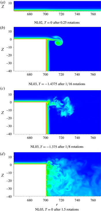
All simulations were started with the laminar von Kármán boundary layer, and for case NL03 a linearly decreasing azimuthal velocity from the wall initialized the flow on the vertical edge of the disk. The simulations with the symmetric boundary condition (L02, NL02) and physical edge (NL03) were run for some time to allow the flow to develop to either a stable radial jet (symmetric condition) or to a developed boundary layer on the finite vertical edge of the disk. Both of these initial conditions are seen in figure 5 where the azimuthal velocity is shown normalized by the disk speed. Figure 5(a) shows the initial condition for NL02. This initial condition was achieved by running the simulations for 0.25 rotations and the flow shown is steady in time. Figure 5(d), on the other hand, shows the initial condition for NL03. This was obtained after running the simulations for 1.5 rotations during which the flow developed. Initially, a radial jet emanated from the edge of the disk, as in (b), and is shown in (c) to break down. After only 0.25 rotations a fully developed boundary layer on the vertical edge of the disk was established, however the simulation was continued in order to see if the turbulence at this edge could act as an upstream disturbance and enter the boundary layer on the disk surface. Despite the turbulence on the vertical part, after 1.5 rotations the boundary layer on the disk surface was still laminar. However, we cannot exclude the possibility that at a later time transition on the disk would be induced from the edge, but we have shown that this is not an immediate process.
Initial conditions for simulations (a) NL02 (the disk edge is at
 $r=700$
) and (d) NL03 showing only part of the full domain. The base flow for L02 is the same as the initial condition for NL02 with a shift in the radial edge position to
 $r=680$
. The azimuthal velocity is shown normalized by the local disk speed, where red corresponds to one and blue to zero. (b,c) Shows the radial jet prior to the development of the turbulent boundary layer on the finite vertical edge of the disk.

All boundary layers were excited by an impulse as described in Appelquist et al. (Reference Appelquist, Schlatter, Alfredsson and Lingwood2015a
) with an excitation position located at a radius of
 $r=490$
. The impulse was added as a short volume force spread over a few length units in the radial direction close to the disk surface, fixed in the rotating frame of the disk. In both the
 $r$
and
 $z$
direction, the spatial shape is a Gaussian function, and in the azimuthal direction a sinusoidal wavefunction was introduced. The strength of the forcing is formally defined as
 $$\begin{eqnarray}\displaystyle \unicode[STIX]{x1D702}=\text{Re}[a(r)\cdot b(z)\cdot c(t)\cdot d(\unicode[STIX]{x1D703})], & & \displaystyle\end{eqnarray}$$
when considering the rotating reference frame. In equation (2.8)
 $a$
,
 $b$
and
 $c$
are functions of either space (
 $r$
,
 $z$
) or time (
 $t$
). The separate terms are defined as
 $$\begin{eqnarray}\displaystyle & \displaystyle a(r)=\text{e}^{-\unicode[STIX]{x1D706}(r-r_{ex})^{2}}\text{e}^{\text{i}\unicode[STIX]{x1D6FC}(r-r_{ex})}, & \displaystyle\end{eqnarray}$$
 $$\begin{eqnarray}\displaystyle & \displaystyle b(z)=\text{e}^{-\unicode[STIX]{x1D707}(z-z_{ex})^{2}}, & \displaystyle\end{eqnarray}$$
 $$\begin{eqnarray}\displaystyle & \displaystyle c(t)=(1-\text{e}^{-\unicode[STIX]{x1D70E}t^{2}})\text{e}^{-\unicode[STIX]{x1D70E}t^{2}}, & \displaystyle\end{eqnarray}$$
 $$\begin{eqnarray}\displaystyle & \displaystyle d(\unicode[STIX]{x1D703})=\text{e}^{\text{i}\unicode[STIX]{x1D6FD}(\unicode[STIX]{x1D703})}. & \displaystyle\end{eqnarray}$$
 $r_{ex}=490$
and
 $z_{ex}=0$
set the excitation location of the disturbance in the radial and wall-normal directions, respectively, whereas
 $\unicode[STIX]{x1D706}=0.5$
,
 $\unicode[STIX]{x1D707}=25$
and
 $\unicode[STIX]{x1D70E}=50$
give the extent of the forcing in space (
 $r$
and
 $z$
directions) and time. The wavenumbers in the radial and azimuthal directions are
 $\unicode[STIX]{x1D6FC}=0.213$
and
 $\unicode[STIX]{x1D6FD}=68$
, respectively. The non-dimensional rotation rate of the disk is
 $\unicode[STIX]{x1D6FA}=1$
. The resulting forcing function in cylindrical form is introduced as
 $$\begin{eqnarray}\displaystyle \boldsymbol{f}=\unicode[STIX]{x1D702}(\boldsymbol{U}_{\boldsymbol{d}}-\boldsymbol{U}_{\boldsymbol{s}}), & & \displaystyle\end{eqnarray}$$
where
 $\boldsymbol{U}_{\boldsymbol{d}}$
is the velocity of the disk and
 $\boldsymbol{U}_{\boldsymbol{s}}$
is the current simulation velocity. The excitation lasts for approximately one-sixteenth of a rotation and time (
 $T$
) is measured in rotations from the start of the excitation. The actual starting time of simulation N03 is, therefore,
 $T=-1.5$
since the boundary layer at the edge had to develop. The amplitude of the impulse was increased for simulation NL02 and NL03, where
 $\unicode[STIX]{x1D702}$
was multiplied by a factor of 1000, compared to NL01, allowing for turbulence to initially develop at earlier radial positions. For the simulations based on the linearized equations, the amplitude of the impulse is not of relevance.
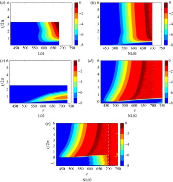
Space–time diagrams showing
 $v_{rms}$
at a height
 $z=1.3$
. All simulations are impulsively disturbed at
 $r=490$
and time zero. The dashed lines in (c,d) indicate the edge of the disk. The logarithmic colour scale is the same for all figures.

3 Results and discussion
In figure 6 space–time diagrams are presented to illustrate the development of the impulse disturbance in all simulations. All figures show the root-mean-square amplitudes
 $$\begin{eqnarray}\displaystyle v_{rms}=\sqrt{\frac{1}{2\unicode[STIX]{x03C0}}\int _{0}^{2\unicode[STIX]{x03C0}}(V_{N}-\overline{V}_{N})^{2}\,\text{d}\unicode[STIX]{x1D703}}, & & \displaystyle\end{eqnarray}$$
where
 $V_{N}$
is the azimuthal velocity normalized by the local disk speed (
 $r\unicode[STIX]{x1D6FA}$
). The root-mean-square values are computed at a height of
 $z=1.3$
and the overbar indicates the mean value in the azimuthal direction. Figures 6(a) L01 and 6(b) NL01 both show globally unstable behaviour, linear and nonlinear, respectively. This behaviour of the flow and the corresponding appearance of the space–time diagrams for L01 and NL01 has previously been discussed in Appelquist et al. (Reference Appelquist, Schlatter, Alfredsson and Lingwood2015a
,Reference Appelquist, Schlatter, Alfredsson and Lingwood
b
). Unstable behaviour then emerges from a small amplitude perturbation where the flow either is affected by the downstream boundary condition (imitating the change of a laminar mean flow to a turbulent one), L01, or actual time-dependent turbulence developing close to the downstream boundary and grows upstream, NL01. The latter indicates a front separating the linear and nonlinear regions moving upstream. In contrast, figures 6(c) L02 and 6(d) NL02 show different behaviours. L02 is linearly globally stable while NL02 is nonlinearly globally unstable. In simulation L02 a high convective radial velocity makes the disturbance leave the domain and at the final time no disturbance is left. Simulation NL02, on the other hand, is disturbed by high amplitude disturbances such that nonlinear effects enter the simulation soon after the excitation. The simulation develops turbulence and again a front is created indicating a separate upstream linear behaviour from a downstream nonlinear behaviour. In the case of NL02 this front moves downstream in contrast to NL01, this is due to the difference in amplitude of the initial impulse disturbance. In figure 6(e) the behaviour for NL03 is the same as in (d) and here it is also possible to see the influence of the edge. Damped disturbances are shown upstream until approximately
 $r=600$
before
 $T=0$
. These disturbances are not amplified in the boundary layer before the impulse is introduced which leads to the same nonlinearly globally unstable behaviour seen emerging for NL01 and NL02.
Nonlinear rotating-disk simulations performed at Tohoku University in Sendai, Japan, with a domain of
 $r=441-570$
, have shown that no disturbances are left inside the domain when perturbed by an impulse (Lee et al.
Reference Lee, Nishio, Izawa and Fukunishi2014). This stable flow is not further considered here.
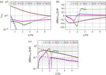
Temporal evolution of root-mean-square and growth rates for all simulations: (a)
 $v_{rms}$
as a function of time at
 $r=530$
and
 $z=1.3$
; (b) growth rates in time of (a); and (c) the same growth rates as in (b) but with absolute values and for an axis in
 $\log _{10}$
scale. Dashed lines are fitted to the last three rotations of the nonlinear cases.

A summary of the amplitudes and growth rates in time for all simulations is provided in figure 7. Values extracted at a height
 $z=1.3$
and radial position
 $r=530$
are shown. In all figures the simulations NL02 and NL03 are hard to distinguish, which essentially means that the flow behaviour on top of the flat plate is independent of the conditions at the disk edge. In figure 7(a) the amplitude of
 $v_{rms}$
is shown, indicating that NL01, NL02 and NL03 are approaching a similar value. The amplitude of L01 grows due to global instability and the amplitude of L02 vanishes eventually due to global stability. Linearly growing behaviour of L01 is assumed for larger times after the simulation was stopped at
 $T=3.25$
, which is shown as a solid line without markers. Figure 7(b) presents the corresponding growth rates in time of the data in figure 7(a) where L01 is assumed to approach a constant value in connection to (a), also as other linear simulations in Appelquist et al. (Reference Appelquist, Schlatter, Alfredsson and Lingwood2015a
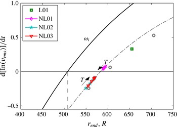
) do. A five value running average was used to evaluate the growth rates mainly because the data of the NL01 simulation were somewhat noisy. The positive growth rate of the NL01 data indicate a growing behaviour in time while approaching zero growth rate for later times, associated with the inward motion of turbulence. The negative growth rates of simulations NL02 and NL03 indicate a decaying behaviour in time associated with the outward motion of turbulence. Also these are seen to approach zero growth rate for later times. An exponential decaying behaviour of the absolute growth rates of NL01, NL02 and NL03 can be identified as shown in figure 7(c) and this indicates that all nonlinear simulations are approaching a zero growth rate at infinite time. For clarification, linearly fitted dashed lines to the last three rotations of the nonlinear cases are also included in the figure.
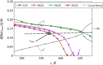
Growth rates in radial direction of
 $v_{rms}$
at the respectively final time of the simulations. Local theory data for the absolute instability are shown as the chain-dotted line as a function of
 $R$
, and for
 $R=655$
the upstream (
 $\unicode[STIX]{x1D6FC}_{i}^{-}$
) and downstream (
 $\unicode[STIX]{x1D6FC}_{i}^{+}$
) modes contributing to the absolute instability with constant
 $\unicode[STIX]{x1D714}_{g}=-13.78+\text{i}0.9810$
are shown as grey lines. Also the upstream mode for the absolutely unstable position
 $R=582.8$
is included with constant
 $\unicode[STIX]{x1D714}_{g}=-15.56+\text{i}0.5680$
. The position
 $r_{end}=570$
is indicated in the figure where
 $r_{end}$
is defined as the intersection between simulation data and local theory data.

To proceed with the analysis, the spatial growth rates at the final time of all unstable simulations are compared in figure 8. The L01 curve does not change in time since the downstream ‘imitated’ turbulence at the end of the domain is stationary. Following Appelquist et al. (Reference Appelquist, Schlatter, Alfredsson and Lingwood2015a
,Reference Appelquist, Schlatter, Alfredsson and Lingwood
b
), the theoretical line for absolutely unstable behaviour is included (
 $\unicode[STIX]{x1D714}_{i}>0$
for
 $R>507$
) in the figure, together with the two modes pinching to create the absolute instability at
 $R=655$
. These modes have constant global frequency
 $\unicode[STIX]{x1D714}_{g}=-13.78+\text{i}0.9810$
(the relation between local,
 $\unicode[STIX]{x1D714}_{l}$
, and global frequency is
 $\unicode[STIX]{x1D714}_{g}=\unicode[STIX]{x1D714}_{l}\cdot R$
, where the local frequency is obtained from local linear theory). Subscripts for imaginary (
 $i$
), real (
 $r$
), global (
 $g$
) and local (
 $l$
) are further used when needed. The simulation data from L01 follow the upstream global mode closely from
 $r=R=655$
, indicated by
 $\unicode[STIX]{x1D6FC}_{i}^{-}$
. This
 $\unicode[STIX]{x1D6FC}_{i}^{-}$
mode is our corresponding linear upstream branch
 $k^{l-}$
mentioned in § 1. For the nonlinear simulation data in figure 8, the global modes are still moving slowly in time. The curve for case NL01 shifts inward and the curves for cases NL02 and NL03 shift outward in relation to the inward or outward shift of the turbulent region. We later show that the cases are approaching the same global mode as
 $T\rightarrow \infty$
. For these curves, the nonlinear data at high
 $r$
are removed. Also for these simulations, it is possible to find a
 $k^{l-}$
branch from the position where the simulation data meet the theoretical line, and in the radially outward direction a
 $k^{nl+}$
branch is expected. The intersection between inward and outward branches is our definition of
 $r_{end}$
where there is a linear region for
 $r<r_{end}$
and a nonlinear region for
 $r>r_{end}$
. The position
 $r_{end}$
was first used by Appelquist et al. (Reference Appelquist, Schlatter, Alfredsson and Lingwood2015a
) to define the end of the linear region, and for case L01 it is stationary in time while for the nonlinear cases it shifts as previously discussed. An indication of
 $r_{end}$
is shown in figure 8 for simulation NL03 at the final time
 $T=6$
for which
 $r_{end}=570$
. The position of
 $r_{end}$
can be mapped in time for these nonlinear simulations, which is further shown in figure 9, and an asymptotic position can then be estimated as
 $582.8$
for the absolute instability, i.e. where the nonlinear lines would collapse and intersect the theoretical line. This
 $\unicode[STIX]{x1D6FC}_{i}^{-}$
mode pinching at
 $R_{cg}=582.8$
(defined as the critical Reynolds number for the global nonlinear flow) is also included in figure 8 having a constant
 $\unicode[STIX]{x1D714}_{g}=-15.56+\text{i}0.5680$
(only shown for
 $R<R_{cg}$
). Note that the various
 $r_{end}$
positions are within the absolutely unstable region (
 $r_{end}>R_{cl}=507$
). The
 $k^{l-}$
branch (our
 $\unicode[STIX]{x1D6FC}_{i}^{-}$
mode) will thus partially lie in the absolutely unstable region for our simulations, which is not consistent with the theory of Pier et al. (Reference Pier, Huerre, Chomaz and Couairon1998) for the elephant mode where
 $r_{end}\rightarrow 507$
for
 $T\rightarrow \infty$
would be expected in order to have the
 $k^{l-}$
branch in the purely convective region.
Growth rates in time as a function of
 $r_{end}$
. The final growth rate of the linear simulations presented in Appelquist et al. (Reference Appelquist, Schlatter, Alfredsson and Lingwood2015a
) are shown as circles. The square shows the linear simulation also presented in this paper, L01. The nonlinear simulations show growth rates between
 $T=3-6$
where the arrows indicates the direction of time. The black line shows
 $\unicode[STIX]{x1D714}_{i}$
from linear theory when
 $\unicode[STIX]{x1D6FD}=68$
(following the absolute instability for
 $\unicode[STIX]{x1D714}_{i}>0$
). This theoretical line is lowered (grey chain-dotted line) to be used as a model to fit the nonlinear data. The dashed line shows the position of
 $R_{cl}=507$
.

Figure 9 shows temporal growth rates as a function of its
 $r_{end}$
. The linear simulation L01 is shown as a square, and circles refer to the additional linear simulations that have been performed in Appelquist et al. (Reference Appelquist, Schlatter, Alfredsson and Lingwood2015a
). For the nonlinear simulations, the growth rate in time at the specific location of
 $r_{end}$
is shown as a function of
 $r_{end}$
. This data have been traced for the last three rotations and an arrow indicates the direction of time. The symbols are plotted equidistant in time, indicating that the propagation of the line is slowing down, consistent with the exponential decaying behaviour of the absolute growth rates. Including data from linear theory for
 $\unicode[STIX]{x1D6FD}=68$
as a line, the critical Reynolds number for absolutely unstable behaviour,
 $R_{cl}=507$
, can be found where
 $\unicode[STIX]{x1D714}_{i}$
changes sign, which is indicated by a dashed vertical line in the figure. The line for the local theory is also shifted by subtracting
 $\text{d}[\ln (v_{rms})]/\text{d}t=0.568$
(grey chain-dotted line), and it clearly follows the trend of the nonlinear simulation data. Lowering this curve even further would result in it following the data of the linear simulations. This empirical approach seems to serve as a good model for our data. Previously, in Appelquist et al. (Reference Appelquist, Schlatter, Alfredsson and Lingwood2015b
), a straight line was fitted to the nonlinear data of NL01 to estimate the asymptotic front position to be at
 $r_{end}=582$
, i.e. where a change of sign took place for the temporal growth. In Appelquist et al. (Reference Appelquist, Schlatter, Alfredsson and Lingwood2015a
),
 $r_{end}=594$
was estimated by linear interpolation by using the linear simulation data. However, here, following our model line based on
 $\unicode[STIX]{x1D714}_{i}$
from linear theory, the position of
 $r_{end}=582.8$
is found from the nonlinear simulations. The aim for all of these approaches has been to obtain an intersection where the critical Reynolds number for the global instability can be defined,
 $R_{cg}$
, similar to how it is defined for local theory. Here it is suggested that our global flow is governed by the absolute instability properties at
 $R_{cg}=582.8$
.
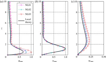
Fluctuation intensity as a function of wall-normal position evaluated from the root-mean-square values in each direction,
 $r$
,
 $\unicode[STIX]{x1D703}$
and
 $z$
, (a)–(c). In each figure, data from the nonlinear simulations NL01, NL02 and NL03 at positions
 $r=589$
,
 $r=570$
and
 $r=570$
, respectively, and local theory data at position
 $R=582.8$
are plotted. The theoretical data correspond to
 $\unicode[STIX]{x1D714}=-15.56+i0.5680$
,
 $\unicode[STIX]{x1D6FC}=0.2088-0.1246$
and
 $\unicode[STIX]{x1D6FD}=68$
. The profiles are normalized by the maximum value of the azimuthal profile (b) for theory and simulations separately.

The local theory eigenfunctions at
 $R_{cg}=582.8$
are compared to the root-mean-square vertical profiles obtained from the simulations at
 $r_{end}=570$
for cases NL02 and NL03, and at
 $r_{end}=589$
for case NL01. The result is provided in figure 10 where all profiles are normalized by the maximum value of the azimuthal velocity for theory and simulations separately. The shape of all profiles in each plot corresponds well, however, the amplitudes differ. Cases NL01 and NL02 have similar amplitudes, whereas NL03 has a higher maximum for
 $u_{rms}$
and
 $w_{rms}$
. The reason for this could be the differences in boundary conditions at the edge of the disk. For all simulations, the mean flow field corresponds to the von Kármán field within the linear region, i.e. for
 $r<r_{end}$
. However, due to the various boundary conditions, the mean flow field over the edge of the disk,
 $r>700$
, is significantly different. For case NL03, there is a negative mean vertical velocity, which is not possible in the other two cases, where fluid is entrained into the boundary layer from the vertical edge of the disk. This could possibly have an upstream effect on the amplitude of the perturbation velocities.
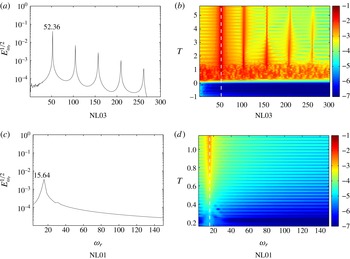
Frequency analysis of the flow: (a) shows the square root of the spectral energy of the signal at
 $r=610$
and
 $z=1.3$
calculated over the last two rotations from case NL03 in the laboratory frame of reference; (b) shows a frequency–time diagram at position
 $r=610$
and
 $z=1.3$
including the amplitude of log
 $_{10}$
(
 $E_{\unicode[STIX]{x1D714}_{r}}^{1/2}$
). The white dashed line is located at
 $\unicode[STIX]{x1D714}_{r}=52.36$
. (c,d) Analogous to (a,b) but including only the linear initial behaviour of NL01 in the rotating frame of reference. The white dashed line is located at
 $\unicode[STIX]{x1D714}_{r}=15.64$
in (d).

In a next step, the temporal frequency can also be analysed. Figure 11 shows various plots of the temporal frequency found for simulations NL03 (a,b) and NL01 (c,d). Case NL02 shows the same behaviour as NL03 and is therefore not explicitly shown. The simulations NL02 and NL03 were made in the laboratory frame of reference such that the signal from the flow field was collected in an analogous way to that measured by a hot-wire probe in an experimental flow field. Simulation NL01 was performed in the rotating frame of reference. In figure 11(a) a Fourier analysis is provided of the signal at
 $r=610$
and
 $z=1.3$
for the last 1.28 rotations of simulation NL03 including 4096 data points. A clear peak at a frequency of 52.36 is identified together with related higher harmonics. Only including the linear initial behaviour of NL01, and for this case using data from
 $T=1$
to
 $T=1.3$
over 1024 data points gives a peak frequency seen in figure 11(c) of 15.64. These waves are moving in the negative
 $\unicode[STIX]{x1D703}$
direction and thus have
 $0>\unicode[STIX]{x1D714}_{rg}=-15.64$
. Knowing the wavenumber
 $\unicode[STIX]{x1D6FD}=68$
of the simulations, the frequencies can be translated between reference frames and are found to correspond, i.e.
 $52.36{-}68=-15.64$
. Translating the absolute mode frequency at
 $R=582.8$
from local linear theory,
 $\unicode[STIX]{x1D714}_{rl}=-0.0267$
to the global reference frame via
 $\unicode[STIX]{x1D714}_{rg}=\unicode[STIX]{x1D714}_{rl}\cdot R$
gives
 $\unicode[STIX]{x1D714}_{rg}=-15.56$
. This value is very close to the frequency obtained in the simulations differing only by 0.08. Slightly different values were also found from the linear simulations in Appelquist et al. (Reference Appelquist, Schlatter, Alfredsson and Lingwood2015a
) where the frequencies for the global modes were increased compared to theory by 0.3–0.4.
In figures 11(b) and 11(d) data are shown after processing the signal at position
 $r=610$
and
 $z=1.3$
to extract the time development of the frequency. The square root of the energy content for each frequency is shown in colour (
 $E_{\unicode[STIX]{x1D714}_{r}}^{1/2}$
) where a moving window in time of 1024 points was included in the Fourier analysis (there were 3600 points per rotation). The wave pattern appearing in the direction of time is due to the number of points used (1024), which was chosen to optimize the algorithm for the Fourier analysis and not for the wavelength to fit exactly within the moving window of analysis. In both figures, the frequency–time diagrams show clear peaks at either
 $\unicode[STIX]{x1D714}_{r}=52.36$
or
 $\unicode[STIX]{x1D714}_{r}=15.64$
, with only slight variations at early times,
 $T<0.5$
. Figure 11(b) also features peaks for the nonlinear harmonics whereas the initial linear behaviour is only seen in 11(d) showing one single peak at all times. Both these figures suggest that the global frequency from the absolute mode at
 $R_{cg}$
is found early on in the simulation. This global frequency may be tuning the flow field to its particular global mode, creating a front according to where this mode matches a local absolute instability. The global frequency is found to be independent of the type of boundary conditions and mesh configurations. Also, when taking the radial direction into account, the same global frequency can be found at all positions for
 $T>0.5$
. It is most likely, therefore, that the presence of turbulence triggers the global frequency.
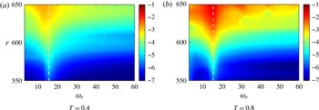
Amplitude
 $\log _{10}$
(
 $E_{\unicode[STIX]{x1D714}_{r}}^{1/2}$
) for the temporal frequencies of signals at different radial positions (
 $z=1.3$
). The frequencies are calculated over a window of 0.32 rotations from case NL01 in the rotating frame of reference at two different times. The white dashed lines indicate
 $\unicode[STIX]{x1D714}_{r}=15.64$
.

With regard to the frequency at each radial position, the simulation NL01 was examined more closely for earlier times with the aim of detecting any possible detuning effect (Davies et al.
Reference Davies, Thomas and Carpenter2007). Figures 12(a) and 12(b) show
 $E_{\unicode[STIX]{x1D714}_{r}}^{1/2}$
for the radius–frequency plane for
 $T=0.4$
and
 $T=0.8$
, and in (a) there is a shift of frequency with radius towards lower frequencies. This same effect is seen in Davies et al.’s (Reference Davies, Thomas and Carpenter2007) figure 3(a) where the frequencies are shown as negative. However, this effect is soon lost, and in figure 12(b), i.e. at later times, no such behaviour is present, although, for the largest radial positions nonlinearities are already present, possibly contaminating the whole flow domain inhibiting the detuning behaviour. The linear variation of frequency with radius promoting global stability explained in Davies et al. (Reference Davies, Thomas and Carpenter2007) is thus shown here to be quickly overtaken by our global frequency.
The square root of energy content,
 $E_{\unicode[STIX]{x1D6FD}}^{1/2}$
, for selected azimuthal wavenumbers as a function of radial position, case NL03. The position
 $r_{end}=570$
(thick dashed line) estimates the boundary between the linear and nonlinear behaviour of the flow field.

Looking at the modal energy in space rather than in time, figure 13 examines the spatial waves found in NL03 at the last time step of the simulation. The possible waves are adapted to the azimuthal extent of the domain appearing as multiples of wavenumber 68. Figure 13 shows the square root of energy content,
 $E_{\unicode[STIX]{x1D6FD}}^{1/2}$
, of the azimuthal wavenumbers as a function of radial position. It is clear that several nonlinear harmonics are present in the flow field at
 $r_{end}=570$
. Imayama et al. (Reference Imayama, Alfredsson and Lingwood2013) defines the transition Reynolds number where the first harmonic in the spectra reaches an amplitude of
 $10^{-6}$
. The orders of magnitude in their spectra are comparable to the amplitudes of figure 13 (the sum of their spectra result in the dimensional value
 $v_{rms}^{\ast }$
, which becomes non-dimensional when dividing by
 $r^{\ast }\unicode[STIX]{x1D6FA}^{\ast }$
which in their case is of order 1) and it can be seen that the value
 $10^{-6}$
is just around
 $r_{end}=570$
for the first harmonic. However, there is a difference since Imayama et al. (Reference Imayama, Alfredsson and Lingwood2013) was referring to the first harmonic of the stationary vortices and here the first harmonic is of a travelling disturbance. For our purposes, this position
 $r_{end}=570$
, where the first harmonic reaches
 $10^{-6}$
, is defined to separate the linear from the nonlinear behaviour. Figure 14 shows a snapshot from the last time step of NL03 in the laboratory frame of reference. The mean velocity hides the perturbation at
 $r_{end}=570$
, which is indicated with a dashed line, but as the perturbation grows stronger with radius it is shown more clearly. The position of
 $r_{end}=570$
can be seen as a position where the flow is constantly perturbed, creating damped waves upstream and amplified waves downstream which eventually break down to turbulence.
Snapshot of the last field of NL03 (
 $T=6$
) at
 $z=1.3$
showing the azimuthal velocity (
 $V$
) in the laboratory frame of reference in logarithmic scale. The black dashed line shows
 $r_{end}=570$
.

The case NL03 is very similar to a real experimental set-up with the edge of the disk at
 $r=700$
. A limitation is the azimuthal periodicity giving the fundamental mode with wavenumber 68. It has been shown for NL03 that such a disk can be run purely with the von Kármán flow without picking up any disturbance from the vertical outer edge for 1.5 rotations. In an experimental set-up, however, this is highly unlikely since there are not only disturbances from the vertical outer edge but also from the free stream and from roughness on the disk surface. To have a completely smooth disk as in DNS would be impossible for experiments even in a clean laboratory environment. Due to these different disturbance environments, case NL03 differs significantly from experiments:
 $r_{end}$
approaches
 $R_{cg}=583$
, which does not match the experimentally observed location for the onset of nonlinearity,
 $R=502-514$
(Lingwood Reference Lingwood1996) and
 $R=510-520$
(Imayama et al.
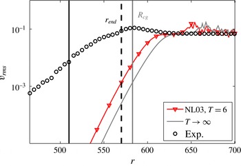
Reference Imayama, Alfredsson and Lingwood2013). This suggests that other disturbances, mainly the stationary vortices, present in all experiments to a greater or lesser degree, modify the flow leading to an earlier onset of nonlinearity and thus an earlier transition point. A comparison is provided in figure 15 (as a grey line) where an estimation of how the final neutral front for
 $T\rightarrow \infty$
is shown. The data shown are the
 $v_{rms}$
modelled on the data from simulation NL03 at
 $T=6$
. Also
 $r_{end}=570$
is indicated as a black dashed line, and to the right, parallel to this line, a grey line indicates the position of
 $R_{cg}=583$
, which is found to be the critical Reynolds number for the global instability. Experimental data are shown for clean-disk experiments (Imayama et al.
Reference Imayama, Alfredsson and Lingwood2014, case IP02) where nonlinearities are entering at
 $R=510$
, denoted here with a black line. Comparing our
 $R_{cg}$
to the position where nonlinearities enter for experimental data, there is a difference in radius of
 $\unicode[STIX]{x0394}r=73$
. There are travelling modes observed in experiments (Imayama et al.
Reference Imayama, Alfredsson and Lingwood2013) just as we observe the travelling global mode from the simulations. The origin of these could be due to turbulence, as in the current study, although the mechanism sustaining the turbulence in experiments may well be the convective stationary vortices due to small distributed roughnesses on the disk surface, which themselves can be susceptible to secondary instabilities. Even though the
 $R_{cl}$
found by Lingwood (Reference Lingwood1995) for the onset of the absolute instability agrees well with the experimentally observed positions for the onset of nonlinearity for relatively smooth disks, both the findings from Appelquist et al. (Reference Appelquist, Schlatter, Alfredsson and Lingwood2015a
) and here (where in both cases the disk is perfectly smooth) suggests that the nonlinear global mode develops further downstream, at least in the absence of stationary vortices.
The azimuthal fluctuation intensity,
 $v_{rms}$
, as a function of
 $r$
for NL03 at time
 $T=6$
and
 $z=1.3$
shown together with the position
 $r_{end}=570$
(thick dashed line), which estimates the boundary between the linear and nonlinear behaviour of the flow field. An estimation based on these data for the neutral nonlinear global front, seen for
 $T\rightarrow \infty$
, is given as a grey line along with
 $R_{cg}$
. Finally, experimental data are also included in the figure (case IP02 in Imayama et al.
Reference Imayama, Alfredsson and Lingwood2014) together with their line for onset of nonlinearity at
 $R=510$
.

4 Summary and conclusions
The boundary layer on an infinitely large rotating disk is linearly globally stable (Davies & Carpenter Reference Davies and Carpenter2003) unless turbulence is modelled downstream, in which case it can be linearly globally unstable (Appelquist et al. Reference Appelquist, Schlatter, Alfredsson and Lingwood2015a ). In this paper, linearly globally stable and unstable flows resulting from differences in set-up and configurations are considered, and it is shown that both are nonlinearly globally unstable.
A number of different simulations, both using the full nonlinear Navier–Stokes equations and their linearized version about the von Kármán base flow, were considered in the present paper. The linear simulation L01 had a sponge region as an outer radial boundary condition modelling the effect of the turbulent outer annulus on an inner region of linear flow. This simulation is shown to be globally unstable, just as the corresponding nonlinear simulation NL01, also using a sponge boundary condition. The linear simulation L02 was, however, shown to be globally stable. This set-up was comparable to an infinitely thin disk, and its corresponding nonlinear simulation NL02 was shown to be globally unstable. The behaviour of case NL03 was globally unstable, just as NL02, however this simulation is easily compared with physical experiments due to the inclusion of the edge of the disk.
Our linearly globally unstable simulation, case L01, resulted in one global mode with a frequency and radial growth rate determined by the position of the artificial turbulence modelled at the outer radial boundary. Our nonlinearly globally unstable simulations, cases NL01, NL02 and NL03, showed asymptotic behaviour approaching the same global mode independent of set-up and configuration. Defining
 $r_{end}$
as the boundary between the linear and nonlinear behaviour, it could be shown that an upstream linear global mode is found to originate from the absolute instability at this
 $r_{end}$
position when observing the radial growth rate. This linear mode corresponds to our
 $k^{l-}$
branch. For the nonlinear behaviour
 $r>r_{end}$
, when harmonics of the travelling mode were observed to exceed an amplitude in
 $\sqrt{E_{\unicode[STIX]{x1D6FD}}}$
of
 $10^{-6}$
, a
 $k^{nl+}$
branch is expected prior to turbulence. The global frequency
 $\unicode[STIX]{x1D714}_{rg}$
for the nonlinear simulations corresponds well to an upstream mode originating from the time-asymptotic position found at
 $R_{cg}=583$
, i.e. where all the nonlinear simulations would collapse on with the same global mode. Interestingly, the temporal frequency
 $\unicode[STIX]{x1D714}_{rg}$
is found and fixed at early times whereas the radial growth rates adapt throughout the simulations. It is suggested that the turbulence triggers this global frequency and the corresponding upstream global mode adapts in time. However, for the linear simulations there is no possibility for the upstream mode to adapt in time since the turbulence is modelled at a fixed position, thus the global frequency is instead set from the absolute instability resulting from the turbulence position. In either case, there is no global instability unless there is downstream turbulence. This also suggests that the infinite disk of Davies & Carpenter (Reference Davies and Carpenter2003) would be globally unstable if downstream turbulence had been included.
The correspondence to an upstream mode from local linear theory suggests an ‘elephant mode’ arising at
 $R_{cg}$
, since by definition the characteristics of the elephant mode are set by local linear theory. The elephant mode acts as a wave maker with an upstream damped wave and a downstream wave that saturates and becomes turbulent fast, possibly because in the nonlinear region the secondary instabilities are absolutely unstable. In the flow field, the nonlinear global mode takes the shape of a neutral front with vanishing temporal growth rate, separating the linear and the nonlinear regions. Since the upstream part of the absolutely unstable domain is ‘pulling’ the elephant mode upstream, it is said to be a pulled nonlinear global mode. The global mode is, however, not pulled the entire way to
 $R_{cl}$
in our simulations, which therefore does not conform precisely to the definition of an elephant mode, i.e. our
 $k^{l-}$
branch is still in the absolutely unstable region. Figure 9 shows this discrepancy between
 $\unicode[STIX]{x1D714}_{i}$
and
 $\text{d}[\ln (v_{rms})]/\text{d}t$
. We suggest that it is not pulled the entire way because of the frequency selection by the turbulence. Taking away this frequency-selection ability from the elephant mode, i.e. taking into account that our simulations exhibit the nonlinear front further downstream than expected (at 583 rather then 507), our elephant mode corresponds well to the findings of Viaud et al. (Reference Viaud, Serre and Chomaz2011) for the rotating cavity. The strong influence of turbulence (though not explored further here) on the transition behaviour requires a different perspective to be taken that accounts for the upstream/inward effects of turbulence on the linear regime. In addition to the above findings, an indication of the detuning effect (Davies et al.
Reference Davies, Thomas and Carpenter2007) was found for early times suggesting that this effect is purely linear and is most effective in an unconfined domain.
An interesting finding is that the vertical edge turbulence of case NL03 did not penetrate the boundary layer within at least 1.5 rotations. The effect on transition between this edge condition and the other cases when adding an impulse was also negligible. It is possible, though, that the different amplitudes of the eigenfunctions in
 $r$
and
 $z$
relate to the edge condition. The configuration of case NL03 makes it easy to compare with experiments and, for example with regards to figure 15, it is suggested that the experiments do not experience the same global instability as the simulations. In experiments it is not possible to have a perfectly smooth disk and the differences in figure 15 are probably due to the stationary vortices modifying the flow. The stationary vortices are themselves susceptible to instabilities and the transition scenario in experiments is likely to include these secondary instabilities. To describe the precise transition scenario an extensive investigation of secondary instabilities is needed, and further simulations are planned to investigate the interactions between the various instability modes.
The main findings of the present paper can be summarized as follows.
-
(i) The simulations have established a critical Reynolds number for the nonlinear global instability to be
 $R_{cg}=583$
, which has a corresponding value of
$R_{cl}=507$
for the local linear absolute instability.
-
(ii) For the nonlinear global instability, the downstream turbulence triggers the frequency for the absolute instability mode found from linear theory at
$R_{cg}$
. -
(iii) At
$R_{cg}$
, where the linear flow is separated from the nonlinear disturbances, an elephant mode is established. -
(iv) There is no influence of disk-edge geometry on
$R_{cg}$
. -
(v) In an experiment, stationary vortices triggered by unavoidable roughness on the surface lead to a different transition scenario and hence the global instability seen in the simulation has not been observed in experiments.


Acknowledgements
This work is supported by the Swedish Research Council through the ASTRID project and the Linné FLOW Centre. Computer time was provided by the Swedish National Infrastructure for Computing (SNIC). Discussions with S. Imayama and B. Pier are gratefully acknowledged. Gratitude also goes to the Professor Fukunishi group at Tohoku University in Sendai, Japan, and especially Dr Nishio for sharing research results of their rotating-disk simulations. E.A. acknowledges ‘The Tetra Pak Award in High Performance Computing’ administered by the Swedish National Committee in Mechanics for funding a three week research visit to Tohoku University in Sendai.