2. Mathematical models and their features

2.1. Governing equations

The models we use are composed of a system of coupled nonlinear partial differential equations for two variables (TV), given by

(2.1) \begin{equation} \frac {\partial }{\partial t} \begin{bmatrix} u \\ v \end{bmatrix} + \mathcal{L} \begin{bmatrix} u \\ v \end{bmatrix} + \epsilon \mathcal{N} \begin{bmatrix} u \\ v \end{bmatrix} = \nu \frac {\partial ^2}{\partial x^2} \begin{bmatrix} u \\ v \end{bmatrix} \text{,} \end{equation}

where $u(x,t)$ and $v(x,t)$ are the two dependent variables, while $x$ and $t$ represent space and time as independent variables, respectively. The right-hand side term in (2.1) represents dissipation, where $\nu$ is viscosity. The nonlinear terms $\mathcal{N}[u\ v]^T = [N_1(u,v)\ N_2(u,v)]^T$ in (2.1) consist of quadratic expressions $N_1$ and $N_2$ , and $\epsilon$ controls the strength of nonlinear terms. Here, $\mathcal{L}[u\ v]^T$ represents the linear dispersive term, which we set $\mathcal{F} ( \mathcal{L} [u \ v]^T ) = \begin{bmatrix} -\omega (\boldsymbol{k}) \hat {v}_k \ \omega (\boldsymbol{k}) \hat {u}_k \end{bmatrix}^T$ , where ( $\hat {u}_k, \hat {v}_k$ ) is the Fourier transform ( $\mathcal{F}$ ) of ( $u,v$ ). We use bold text for wavenumbers, such as $\boldsymbol k$ , that can take positive and negative values, while magnitudes of the wavenumbers will be denoted without bold text, such as $k$ .

Ignoring the nonlinear and dissipation terms temporarily, (2.1) in Fourier space is $\partial \hat {u}_k /\partial t - \omega (\boldsymbol k) \hat {v}_k = 0$ and $\partial \hat {v}_k/ \partial t + \omega (\boldsymbol k) \hat {u}_k = 0$ . Manipulating these equations further gives $ ( \partial ^2/\partial t^2 + \omega ^2(\boldsymbol k) ) [\hat u_k, \hat v_k]^T=0$ . This shows that each Fourier mode oscillates at frequency $\omega$ which is a function of wavenumber, $\boldsymbol k$ , based on the dispersion relationship. As a result, the linear inviscid partial differential equations have dispersive waves as their solution.

2.2. Nonlinear terms

We consider two distinct forms of nonlinear expressions for $N_1$ and $N_2$ as

(2.2) \begin{align} \underbrace { \begin{bmatrix}N_1 \\ N_2 \end{bmatrix} = \begin{bmatrix} uv_x + 2vv_x \\ vu_x + 2uu_x \end{bmatrix} }_{{TV1}}\quad \text{and }\quad \underbrace { \begin{bmatrix}N_1 \\ N_2 \end{bmatrix} = \begin{bmatrix} uv_x - 2vv_x \\ -vu_x + 2uu_x \end{bmatrix} }_{{TV2}}\text{.} \end{align}

We chose the above-mentioned quadratic nonlinear forms such that total energy of the system, $E = \int 1/2(u^2+v^2) \,{\rm d}x$ , is conserved in the absence of dissipation, i.e. when $\nu = 0$ . The linear terms in (2.1) therefore are responsible for linear dispersive waves, while the quadratic nonlinear terms give rise to nonlinear interactions and energy transfer across scales.

Here onward, we refer to models described by (2.1) with the first and second forms of nonlinearity as the two-variable models 1 and 2 (TV1 and TV2), respectively. We will explore the turbulent dynamics of these models in a periodic domain, $x \in [0, 2\pi ]$ .

The two kinds of nonlinear terms give rise to different nonlinear dynamics. To see this, we set the linear dispersive terms in (2.1) to zero and integrate the equations in freely evolving configuration for different initialisations. The numerical integration details are described later and, here, we briefly look at some solutions. Results from one example integration, with initial conditions $u(x,0) = v(x,0) = \sin x$ , are shown in figure 1. Panels (a)–(c) show $u$ from the TV1 model while panels (d)–(f) show $u$ from the TV2 model. The $v$ field for these integrations showed qualitatively similar features and are omitted here. In panels (a)–(c), we see that an initial sinusoidal profile steepens and forms a shock with time. For the TV1 model, notice that the setting $u=v$ and scaling time leads to Burgers’ equation, which can form shocks for arbitrary initial conditions. This behaviour is seen in figure 1(a–c). Of course, in general, $u \neq v$ , which means that the TV1 model has richer dynamics than Burgers’ equation for a single variable.

In contrast, we see completely different features for the TV2 model’s results shown in figure 1(d–f). Notice that the initial sinusoidal structure develops fine-scale instabilities at its extreme value points, and these fine-scale structures propagate across and disintegrate the whole field. From this particular experiment and several other experiments we ran, we found that the two models capture widely different nonlinear dynamic behaviours. Since we will be exploring dispersive wave turbulence with different dispersion relationships, it will be useful to have two different kinds of nonlinear interaction terms in the model. This will allow us to check how the dynamics changes with varying nonlinear interaction terms for each dispersive turbulent regime.

Figure 1.

Time evolution of the variable $u$ for the (a)–(c) TV1 and (d)–(f) TV2 nonlinear models, obtained from the non-dispersive form of (2.1). The insets in panels (d)–(f) show zoom-ins on highly fluctuating regions of the field.

2.3. Triadic resonances and dispersion relationships

We constructed different dispersion relationships for the previous models based on triadic resonant interaction possibilities. For three wavenumbers $\boldsymbol{p}$ , $\boldsymbol{q}$ and $\boldsymbol{k}$ , and corresponding frequencies $\omega (\boldsymbol{p})$ , $\omega (\boldsymbol{q})$ and $\omega (\boldsymbol{k})$ , the conditions for three-wave resonance are

(2.3a) \begin{align} \boldsymbol{p} + \boldsymbol{q} + \boldsymbol{k} = 0 \qquad \text{and} \end{align}

(2.3b) \begin{align} |\pm \omega (\boldsymbol{p}) \pm \omega (\boldsymbol{q}) \pm \omega (\boldsymbol{k})| \leqslant \delta. \end{align}

Furthermore, each wavenumber, say $\boldsymbol{k}$ , can take positive and negative values, which is why we do not have $\pm$ in the wavenumber condition in (2.3a ). The term $\delta$ , where $0 \leqslant \delta \ll 1$ , represents a small positive parameter, which allows for near-resonant or quasi-resonant interactions between waves. That is, when $\delta \neq 0$ , the interactions are considered near-resonant, meaning the wave frequencies are close to, but not exactly matching the resonant condition (2.3b ). When $\delta = 0$ , the interactions are exact-resonant, meaning that the wave frequencies exactly match and the frequency condition in (2.3b ) gets modified as $ \pm \omega (\boldsymbol{p}) \pm \omega (\boldsymbol{q}) \pm \omega (\boldsymbol{k}) = 0$ .

For each model, TV1 and TV2, we set up four dispersion relations as: (a) Sine (sinusoidal), $ \omega (\boldsymbol{k}) = \boldsymbol{k} + f \sin { ( \pi \boldsymbol{k} / c )}$ ; (b) Algebraic, $\omega (\boldsymbol{k}) = f\boldsymbol{k} / (c+\boldsymbol{k})$ ; (c) Rossby (Rossby wave), $ \omega (\boldsymbol{k}) = f\boldsymbol{k} / (c + k^2 )$ ; and (d) IG wave (internal gravity wave), $\omega (\boldsymbol{k}) = \pm \sqrt {(f^2 + c^2 k^2) / (1 + k^2)}$ . Here, $f$ and $c$ are parameters that can be varied; the specific values used in this study are listed in table 1.

Table 1.

Parameters used in the study.

The sinusoidal dispersion relation is inspired by the Fermi–Pasta–Ulam–Tsingou (FPUT) system, which describes a one-dimensional (1-D) lattice of coupled harmonic oscillators (Onorato et al. Reference Onorato, Vozella, Proment and Lvov2015; Lvov & Onorato Reference Lvov and Onorato2018; Bustamante et al. Reference Bustamante, Hutchinson, Lvov and Onorato2019; Zaleski, Onorato & Lvov Reference Zaleski, Onorato and Lvov2020). We call the second dispersion relation as the Algebraic dispersion relation because it has an algebraic triadic resonance manifold $\boldsymbol{p} = - (1+ \boldsymbol{k})$ . Except for the discrete values $\boldsymbol{k} \in \{-2, -1, 1\}$ , the resonance manifold contains wavenumbers that satisfy the resonance conditions (2.3) exactly with $\delta = 0$ . The Rossby and IG wave dispersion relations are inspired by dispersive waves in geophysical flows. Specifically, in geophysical flows, we have dispersion relationships $\omega (\boldsymbol{k}) = -\beta \boldsymbol{k}_h / ( K^2 + k_d^2 )$ for Rossby waves and $\omega ^2(\boldsymbol{k}) = ( f_0^2 k_v^2 + N_B^2 k_h^2 ) / ( k_v^2 + k_h^2 )$ for internal gravity waves, where $\boldsymbol{K}$ is the three-dimensional wavenumber such that $K^2 = k_h^2 + k_v^2$ , with $\boldsymbol{k}_h$ and $\boldsymbol{k}_v$ representing the horizontal and vertical wavenumbers, respectively; $\beta , k_d, f_0$ and $N_B$ are parameters involved in the dispersion relations due to rotation and stratification (Pedlosky Reference Pedlosky2003; Vallis Reference Vallis2017). The frequencies of these dispersion relations are bounded: for Rossby waves, $\omega \to 0$ as $|\boldsymbol{k}_h| \to \{0,\infty \}$ , with finite frequencies in between; similarly, for internal gravity waves, $f_0 \leqslant |\omega | \leqslant N_B$ as $0 \leqslant |\boldsymbol{k}_h| \leqslant \infty$ . The Rossby and IG wave dispersion relations considered in this study were constructed incorporating these properties of similar named geophysical waves, with the goal of obtaining triadic wave–wave interactions in one dimension.

Figure 2.

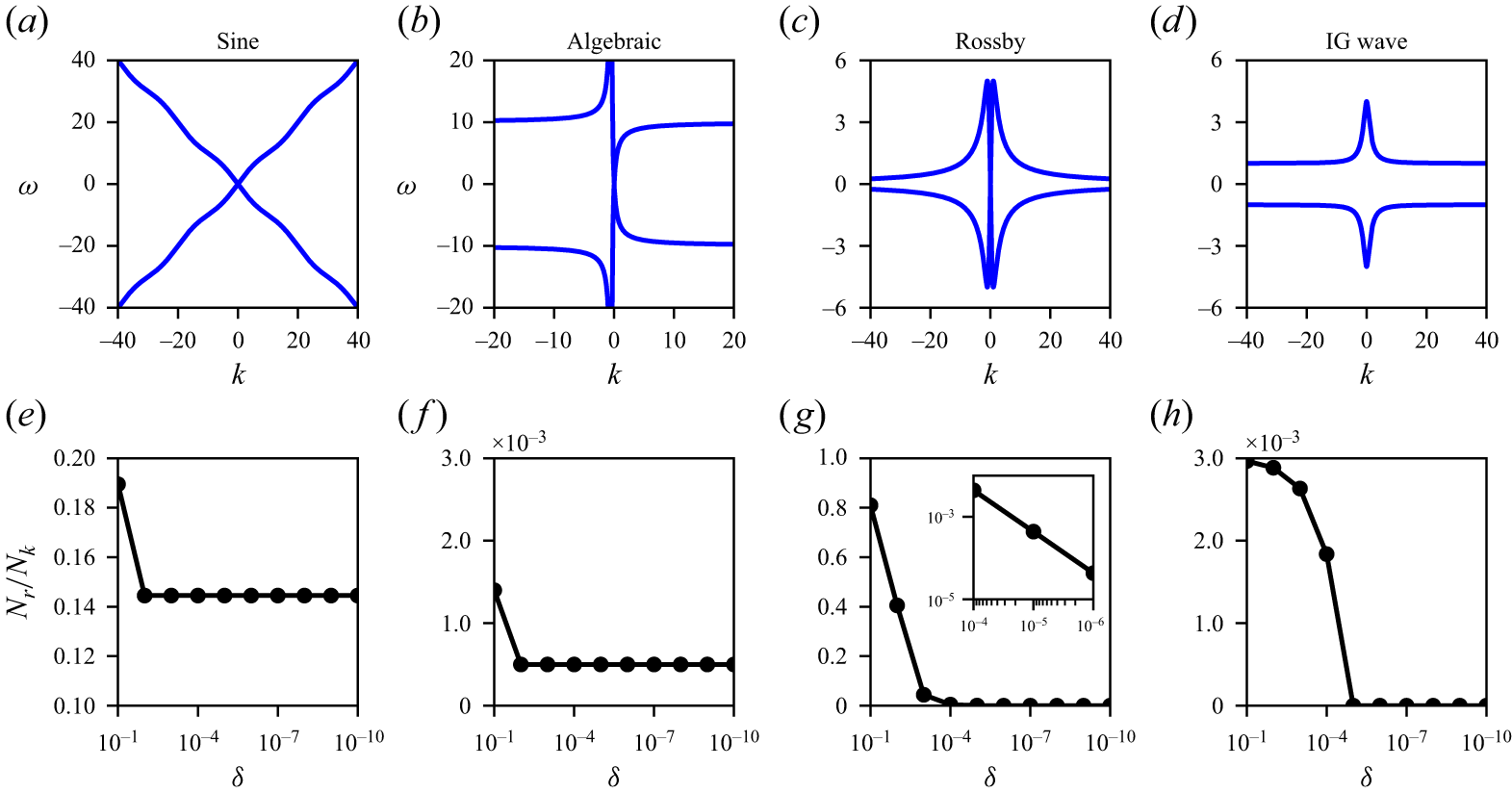
Dispersion curves in $ \omega {-}k$ space are shown for: (a) Sine, (b) Algebraic, (c) Rossby and (d) IG wave cases. The second row shows the fraction of resonant modes to total modes, $N_r / N_k$ , as a function of tolerance $\delta$ ; (e) Sine and (f) Algebraic dispersion relations show convergence to exact-resonance, while (g) Rossby and (h) IG wave relations exhibit near-resonances, with the fraction of resonant modes vanishing with decreasing  $\delta$ .

Figure 3.

Resonant modes ( $k,p$ ) corresponding to dispersion relations as obtained for different tolerances, $\delta$ . Each row represents one of the four dispersion relations and each column corresponds to specific tolerances. Panels (i) and (l) show a larger domain than that shown in previous panels of the last two rows. In panels (d)–(f), the resonance line $\boldsymbol{p} = -(1+\boldsymbol{k})$ corresponding to the Algebraic dispersion relation, as mentioned in the text, maps to two lines in the $(k,p)$ mode space. This is highlighted with an inset in panel (f).

The dispersion curves for the parameters given in table 1 are shown in figure 2(a–d). For the four kinds of dispersion relations, we identified numerous resonant wavenumbers using a brute-force high precision numerical search algorithm such that the wavenumbers satisfy the triadic resonant conditions in (2.3), with the numerical errors being of the order of machine precision, $O(10^{-16})$ . We varied the tolerance $\delta$ from $0.1$ to $10^{-10}$ . Since we consider a $2\pi$ -periodic domain, the wavenumbers are integers. Additionally, as will be seen later, the inertial range of the turbulent flows goes up to a maximum of $k \approx 1000$ . Accordingly, we set out numerical searches with each wavenumber, say $\boldsymbol{k} \in [-1000, 1000] \setminus \{0\}$ . Wavenumber $0$ was excluded since this is the spatially homogeneous mode and is trivially resonant. The total number of wavenumber pairs involved in the search across the four quadrants is then $N_k = ( 2 \times 1000 )^2$ . By gradually reducing the tolerance $\delta$ , we calculated the resonant set fraction $N_r / N_k$ , where $N_r$ is the number of resonant wavenumber sets. The convergence test results of resonant wavenumber sets corresponding to the dispersion relations, i.e. $N_r / N_k$ versus $\delta$ , are shown in figure 2(e–h).

As we see in figures 2(e) and 2(f), the resonant set fraction becomes constant for the Sine and Algebraic dispersion relations at low $\delta$ . It indicates that resonant wavenumber pairs of these dispersion relations converged to exact-resonances. However, $N_r / N_k \to 0$ with decreasing $\delta$ for the Rossby and IG wave relations, as seen in figures 2(g) and 2(h), respectively. These dispersion relations therefore give rise to near-resonances, with no exact resonances.

We extracted wavenumbers $\boldsymbol k$ and $\boldsymbol p$ for all $\boldsymbol q$ from the resonant triads $(\boldsymbol k, \boldsymbol p, \boldsymbol q)$ , and took the absolute value of the wavenumbers, so that the negative wavenumbers also appear in the first quadrant of the $\boldsymbol k {-} \boldsymbol p$ space. Here on, we use the term ‘mode’ to refer to $k = |\boldsymbol{k}|$ . The resonant points in $k{-}p$ mode space are compactly shown in figure 3 for the four dispersion relationships for three different $\delta$ values. From the first two rows, we see that the patterns do not change for $\delta = 0.01$ and $0.001$ in figures 3(b) and 3(c) for the Sine, and figures 3(e) and 3(f) for the Algebraic relation. Thus, the modes present in the converged pattern are exact-resonant modes. Notice that a lot of exact resonant points appear in panel (c) for the Sine case, while the Algebraic case has exact resonances lying along two lines close to the diagonal, as shown in the inset of panel (f). We also see near-resonant modes in panels (a) and (d). In panel (a), we see the near-resonant clusters surrounding exact resonances. In panel (d), we see lines close to $k$ and $p$ axes, these near-resonant points disappearing as we reduce $\delta$ .

For the other two dispersion relations, resonant modes vanish near the origin with reducing $\delta$ , as seen in the last two rows of figure 3. Due to this, panels (i) and (l) show double the domain size shown in previous panels in the last two rows. For the Rossby relation shown in panels (g)–(i), a reduction in tolerance leads to fewer resonant modes, which become increasingly confined to specific directions with decreasing $\delta$ . Additionally, near-origin resonant modes drop out, with near-resonant modes away from the origin remaining. Similar features were observed for the IG wave relation, as shown in panels (j)–(l), where progressively fewer resonant modes remain near the origin as $\delta$ decreases. Lower tolerance cases ( $\delta \lt 10^{-3}$ ) are not shown, as near-resonant modes ultimately diminish for Rossby and IG wave relations as seen in figures 2(g) and 2(h), respectively.

Figures 2 and 3 provide key insights on the features of resonant modes associated with the dispersion relationships. Comparing among the dispersion relationships, we see that the number of resonant modes, including both near- and exact-resonant ones, decreases in the order Sine $\gt$ Rossby $\gt$ IG wave $\gt$ Algebraic. Sine and Algebraic relations support both exact and near-resonant modes, eventually converging to exact resonances with decreasing $\delta$ . However, Rossby and IG wave relations display only near-resonant modes which eventually disappear at very low $\delta$ . These four kinds of dispersion relationships provides us with a good platform to explore how turbulent wave transfers are affected by the different types and distribution of resonant modes.

3. Energy, flux and dissipation

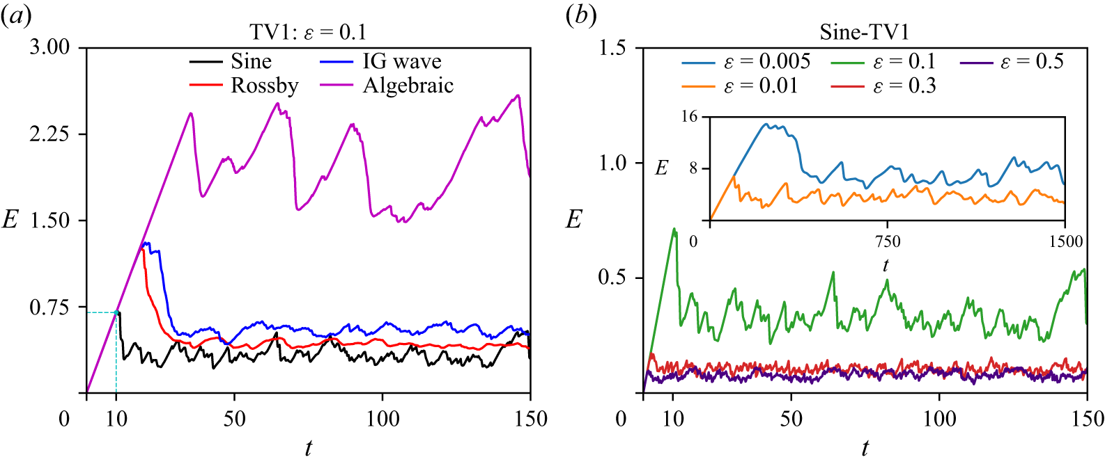
Out of the 40 numerical integrations discussed previously, in figure 4, we show the energy time series ( $E$ versus $t$ ) for selected TV1 model cases. Panel (a) illustrates the effect of varying dispersion relations with $\epsilon$ fixed at 0.1, while panel (b) presents results for varying nonlinearity strengths with the Sine dispersion relation. Each case starts from $E \sim 0$ , although the forcing leads to $E$ monotonically increasing with a constant slope early on, as seen in panel (a). The slope of the straight line is the rate of energy injection, i.e. $\Delta E / \Delta t = 0.7/10 = 0.07$ , this being marked with dashed cyan lines in figure 4(a).

As mentioned earlier, all flow regimes are forced at low wavenumbers, $1 \leqslant |k| \leqslant 3$ . Thus, each system requires some time (depending on $\omega (k)$ and $\epsilon$ ) to transfer the forced energy across the inertial range and eventually to dissipation scales. When the system starts to dissipate energy, $E$ decreases and hence departs from the straight line of slope of 0.07. Once dissipation balances the energy injection, the system achieves a statistically steady state. The steady state energy levels in figure 4(a) for $\epsilon = 0.1$ are in the order: Sine $\lt$ Rossby $\lt$ IG wave $\lt$ Algebraic. Also notice that the steady-state energy level increases with decreasing $\epsilon$ for the Sine-TV1 cases, as seen in figure 4(b). These features will be clearer once the energy transfer across scales is explained in the following sections. All the physical features and other statistical quantities described subsequently are from the steady-state flows.

Figures 5(a) and 5(b) show the variation of the time-averaged domain-integrated energy ( $\bar {E}$ ) as a function of the degree of nonlinear strength ( $\epsilon$ ) for TV1 and TV2 model cases, respectively. We see that $\bar {E}$ increases with decreasing $\epsilon$ . Since the energy injection rate is constant, low- $\epsilon$ systems must inefficiently transfer energy to the dissipation scales, causing energy to grow until dissipation matches injection at steady states. Thus, a lower $\epsilon$ results in a higher $\bar {E}$ . Similar results have been reported in other studies examining rotating and non-rotating shallow water wave turbulence (Augier, Mohanan & Lindborg Reference Augier, Mohanan and Lindborg2019; Thomas, Rajpoot & Gupta Reference Thomas, Rajpoot and Gupta2024).

We next look at spectral energy fluxes. Ignoring dissipation terms temporarily, we computed the Fourier transform of (2.1) and then multiplied it by the complex conjugate of the Fourier transform of $[u\ v]^T$ . Summing the two equations thus obtained and taking its real part gives

(3.1) \begin{equation} \frac {{\rm d}\hat {E}_k }{{\rm d}t} = \hat {R}_k \textit {,} \end{equation}

where $\hat {E}_k = ( |\hat {u}_k|^2 + |\hat {v}_k|^2 )$ is the spectral energy in mode $k$ . Here, $\hat {R}_k = -2 \epsilon {\rm Re} [ \hat {u}_k^* \mathcal{F}(N_1) + \hat {v}_k^* \mathcal{F}(N_2) ]$ is the nonlinear spectral transfer term, where ${\rm Re}$ stands for real part and $*$ denotes the complex conjugate.

The cumulative sum of the transfer term will give the spectral flux $\hat {\varPi }_k$ ,

(3.2) \begin{equation} \hat {\varPi }_k = \varSigma _{\infty }^{k} \hat {R}_k \text{.} \end{equation}

Note that the transfer term $\hat {R}_k$ and hence the spectral flux $\hat {\varPi }_k$ has no contribution from the linear term ( $\mathcal{L}$ ) as the $\pm \omega (k) {\rm Re} [\hat {u}_k^* \hat {v}_k]$ terms will cancel out each other in the energy equation. The energy flux is therefore only due to the nonlinear terms.

Figure 4.

Energy time series for selected TV1 model cases. (a) Time evolution of energy for different dispersion relations, $\omega (\boldsymbol{k})$ , at fixed nonlinearity $\epsilon = 0.1$ . (b) Energy time series for varying nonlinearity levels ( $\epsilon$ ) for the Sine dispersion relation. The inset in panel (b) shows the cases with smaller $\epsilon$ , where energy levels are significantly higher than those for $\epsilon = 0.5$ , $0.3$ and $0.1$ .

Figure 5.

Variation in (a, b) time-averaged energy, (c, d) flux and (e, f) dissipation as a function of $\epsilon$ . Left and right columns correspond to TV1 and TV2 models, respectively.

The time averaged spectral flux ( $\bar {\hat {\varPi }}_k$ ) for Sine-TV1 and Sine-TV2 models are shown in figures 5(c) and 5(d), respectively. As we see, $\bar {\hat {\varPi }}_k$ remains constant for some $k$ -band, which is the inertial range. For all $\epsilon$ cases, the inertial range fluxes are of comparable magnitudes. However, the inertial range shortens as $\epsilon$ decreases, with a staircase like pattern emerging at low $\epsilon$ . The shortening of inertial range is an indication of inefficiency in downscale transfers and an increase in the energy levels at steady states, as pointed out in figures 5(a) and 5(b). The spectral flux corresponding to the other dispersion relations showed similar characteristics to that of the Sine dispersion relation (figures omitted).

Following energy flux, we calculated the domain-integrated energy dissipation at steady state as

(3.3) \begin{equation} D = \nu \int _0^{2\pi } \left ( u \frac {\partial ^2 u} {\partial x^2} + v \frac {\partial ^2 v} {\partial x^2} \right )\, {\rm d}x \text{,} \end{equation}

which is then time-averaged to get $\bar {D}$ . As shown in figures 5(e) and 5(f), the steady-state-averaged dissipation $\bar {D}$ in all cases was close to 0.07, with less than 10 % variation around this value. This matches the constant energy injection rate discussed earlier and reflected in the slope of energy injection during the transient phase seen in figure 4(a). All the flows we set up therefore have a constant energy flow through the system with similar dissipation, although due to varying efficiencies in energy transfer across scales, we have variable total energy in different regimes.

4. Efficiency of the cascade

As seen earlier, although all the flows have the same energy injection rate and forward cascade rate, low- $\epsilon$ flows gain more energy than high- $\epsilon$ flows. To compare these different flows, we construct the notion of ‘efficiency of the energy cascade’ by examining the energy equation. Multiplying (2.1) by $[u\ v]^T$ and summing the two set of equations gives us

(4.1) \begin{equation} \frac {\partial e}{\partial t} + r = d, \end{equation}

where the time derivative of the pointwise energy, $e = 1/2(u^2 + v^2)$ , is balanced by the pointwise energy transfer term, $r$ , and pointwise dissipation, $d$ . While the nonlinear terms are responsible for downscale energy transfer across the inertial range, dissipation acts as the energy sink at grid-scale. Given this, we may think of the ratio of dissipation to the transfer term as an indicator for the efficiency of downscale energy transfers. Assuming $U$ and $L$ represent characteristic velocity and length scales of the system, the transfer term $r$ scales as $U^3 / L$ . We then define pointwise efficiency, $\eta _{\textit{pointwise}}$ , as

(4.2) \begin{equation} \eta _{\textit{pointwise}} \sim \frac {\rm d}{U^3 / L} = \frac {{\rm d}L}{U^3} \text{.} \end{equation}

Figure 6.

Variation in cascade efficiency, $\bar {\eta }$ , as a function of $\epsilon$ across different dispersive models: (a) TV1 and (b) TV2.

We can improve (4.2) by using domain-integrated values instead of the pointwise values. If $D$ and $E$ denote dissipation and energy integrated over the domain, we have $D \sim {\rm d}L$ and $E \sim U^2 L$ . Substituting these into (4.2) and further replacing instantaneous values with time-averaged quantities gives us the expression for cascade efficiency:

(4.3) \begin{equation} \bar {\eta } = \bar {D} \left ( \frac {L}{\bar {E}} \right )^{3/2}. \end{equation}

To compute the efficiency, we chose $L$ as the length of the domain. As seen earlier, the average dissipation rate $\bar {D}$ is more or less constant, while the mean energy, $\bar {E}$ , increases with decreasing $\epsilon$ . This leads to efficiency decreasing with decreasing $\epsilon$ , as seen in figure 6 for both the TV1 and TV2 models. We see that $\bar {\eta }$ decreases by two to four orders of magnitude across different dispersion relations, as $\epsilon$ decreases from 0.5 to 0.005.

5. Energy spectra

Figure 7 shows the time-averaged energy spectra, $\bar {\hat {E}}_k$ versus $k$ , for TV1 and TV2 models. Notice that the spectra are well developed with a long inertial range for $\epsilon =0.5$ . The spectra however become steeper with a smaller constant slope inertial range as we reduce $\epsilon$ , with the steepest spectra being observed for the $\epsilon =0.005$ case. We have added best fit slope lines, using spectra data in the wavenumber interval $k \in [100,400]$ for each panel. Similar to our figures, the steepening of spectra with decreasing nonlinearity has been seen in several previous experimental and numerical studies on rotating and stratified turbulence as applied to geophysical flows (Bartello & Tobias Reference Bartello and Tobias2013; Rodda et al. Reference Rodda, Savaro, Bouillaut, Augier, Sommeria, Joël, Valran, Viboud and Mordant, Nicolas2023; Thomas et al. Reference Thomas, Rajpoot and Gupta2024).

Figure 7.

Energy spectra for TV1 (left column) and TV2 models (right column). The rows represent different dispersion relations, as written on the left. Each panel illustrates the transition of spectra from strong to weakly nonlinear regimes. Two best fit slope lines obtained over the wavenumber range $k \in [100,400]$ are shown in each panel, corresponding to strong ( $\epsilon =0.5$ ) and weak ( $\epsilon =0.005$ ) nonlinearities. The grey highlighted wavenumber bands in the first column are discussed in § 7.

In figure 7, we see that as the constant slope inertial ranges shrink with decreasing $\epsilon$ , similar to flux, as in figures 5(c) and 5(d), the spectra begin to display pronounced oscillations. Additionally, we see that the spectral oscillations in the Sine-dispersive models (figure 7 a,b) are more frequent than the Rossby relation based models (figure 7 e,f). The other two, Algebraic (figure 7 c,d) and IG wave relations (figure 7 g,h) only show limited visible oscillatory peaks. Similar oscillating spectra have also been reported for triadic nonlinear interacting systems in the past (Falkovich & Shafarenko Reference Falkovich and Shafarenko1988; Pushkarev & Zakharov Reference Pushkarev and Zakharov2000; Proment, Nazarenko & Onorato Reference Proment, Nazarenko and Onorato2009). The distinct peaks and valleys in spectra suggest the possibility of underlying patterns in the distribution of energy across different modes. Below we will analyse these oscillatory parts of the spectra in the context of mode-to-mode energy transfers.

It is noteworthy that in the regime of weaker nonlinearity, oscillations are superimposed on a rapidly dropping steep energy spectrum. Despite the fast decay of the spectrum, it is important to note that all the flows have more or less a similar rate of energy transfer from large scales to small scales, due to the nature of the forcing we employed. Although the oscillations and rapid drop in energy make the inertial range difficult to identify from the spectrum alone, its presence is seen in the spectral energy flux (figure 5 c,d), which remains approximately constant over a range of wavenumbers. The rapid drop in spectra at the lowest level of nonlinearity is also not to be confused with dissipative effects. Dissipation remains prominent at the smallest scales or highest wavenumbers, based on the choice of the viscosity we made and once again, the presence of a clean inertial range in spectral flux is an indication of the inviscid inertial range. Given these, the rapid drop in spectra and the emergence of oscillations in the spectra are indicative of inefficient downscale transfer of wave energy at lower levels of nonlinearity, as quantified in the previous section.

6. Transition to linear wave dominated regime

We collected $\hat {u}_k$ and $\hat {v}_k$ over a long time interval, and Fourier transformed them over time to get the frequency–wavenumber spectra $\hat {u}_k^\omega$ and $\hat {v}_k^\omega$ . Figure 8 shows the $|\hat {u}_k^\omega |^2$ for all dispersion relations for the TV1 models with $\epsilon = 0.1$ . Notice that localised high energy bright regions are located close to the dispersion curves (green lines), confirming the presence of linear waves. Two bright columns also appear around $k= 0$ due to the low-wavenumber forcing we used. The $\omega {-}k$ spectrum for $v$ was seen to be similar to those shown for $u$ . Similarly, the frequency–wavenumber spectra for the TV2 models resembled those of the TV1 models (figures omitted).

Figure 8.

Frequency–wavenumber spectra of $u$ from TV1 model with $\epsilon = 0.1$ . The four panels correspond to (a) Sine, (b) Algebraic, (c) Rossby and (d) IG wave dispersion relations. Dispersion relationship curves are drawn with green colour in each panel.

With increasing $\epsilon$ , we found the bright energetic regions to broaden beyond the vicinity of the dispersion curves. To quantify the variation in linear wave energy with $\epsilon$ , we used a filtering approach, similar to that used in multiple past studies (Maffioli, Delache & Godeferd Reference Maffioli, Delache and Godeferd2020; Thomas & Ding Reference Thomas and Ding2023; Labarre et al. Reference Labarre, Augier, Krstulovic and Nazarenko2024). Figure 9(a) shows a schematic of the filtering approach. We set up a narrow band $\pm \delta \omega$ around dispersion curves $\omega (k)$ and define the part of the flow that falls in this narrow band as linear waves. Specifically,

(6.1) \begin{equation} |\hat {u}_k^\omega |^2_L = \begin{cases} |\hat {u}_k^\omega |^2 & \text{if } |\omega - \omega (k)| \leqslant \delta \omega , \\ 0 & \text{otherwise}. \end{cases} \end{equation}

Then, the linear wave energy fraction is calculated as $\bar {E}_L / \bar {E}$ , where $ \bar {E}_L = \sum _{\omega , k} ( |\hat {u}_k^\omega |^2_L + |\hat {v}_k^\omega |^2_L )$ is the linear wave part and $\bar {E} = \sum _{\omega ,k} ( |\hat {u}_k^\omega |^2 + |\hat {v}_k^\omega |^2 )$ is the total energy. We verified that $ \bar {E}_L / \bar {E} \to 1$ as we increase the tolerance $ \delta \omega$ from 0.5 to 10 (see figure 9 b). To enforce a strict metric, we associate the linear wave field with the narrowest band, $\delta \omega = 0.5$ , based on the filtering approach. The fraction using this filtering band is plotted in figures 9(c) and 9(d) for TV1 and TV2 models, respectively.

As we see, the systems shift from a strongly nonlinear state ( $ \bar {E}_L / \bar {E} \sim 15\,\%$ at $ \epsilon = 0.5$ ) to a more linear regime ( $98\,\%$ at $ \epsilon = 0.005$ ) for the Sine-TV1 and TV2 models; notice the black lines. Similar behaviour is seen for other dispersion relations as well (red and blue lines for Rossby and IG wave relation based models, respectively). The maximum linear wave energy fraction obtained for the Algebraic models are ${\sim}50$ , as seen from the magenta-coloured lines. This can be attributed to the broader spread in energy away from dispersion curves even at low $\epsilon$ , as seen in figure 8(b). Overall, these findings reveal transition from a strongly nonlinear flow with less linear wave energy to a WWT flow with a dominant linear wave content as $\epsilon$ decreases from 0.5 to 0.005.

Figure 9.

(a) Schematic of $\omega {-}k$ spectrum filtering for linear wave energy calculation, with a tolerance of $\pm \delta \omega$ around the Sine dispersion relation (represented by the green-coloured line). Regions with width 0.5 and 2.5 on either side of the dispersion curve are coloured in yellow and orange, respectively. (b) Comparison of the linear wave energy fraction between the highest and lowest nonlinear ( $\epsilon$ ) cases for different values of tolerance ( $\delta \omega$ ) in the Sine-TV1 model. (c) and (d) Variation of linear wave energy fraction ( $ \bar {E}_L / \bar {E}$ ) as a function of $\epsilon$ for the TV1 and TV2 models, respectively, with the lowest tolerance of $\delta \omega = 0.5$ .

In addition to the transition seen earlier using the dynamic flow fields, we can also see the same phenomenon by comparing the linear time scales with nonlinear time scales. For this, we will follow a procedure used by Miquel & Mordant (Reference Miquel and Mordant2011). We write the solution of the flow fields at a particular wavenumber $\boldsymbol k$ as $\hat {u}_k = A e^{i \omega (\boldsymbol{k}) t} + B e^{-i \omega (\boldsymbol{k}) t}$ , where $A$ and $B$ are amplitudes, and $\omega (\boldsymbol{k})$ is the linear wave frequency at that wavenumber. This solution satisfies the inviscid linear equations and we define the linear time scale $\tau _{l} =1/\omega$ . By defining the autocorrelation $\mathcal{C}_k(\tau ) = \langle A(t) A^*(t + \tau ) \rangle$ , we can calculate a nonlinear time scale $\tau _{nl} = \int _{0}^{T_\infty } {|\mathcal{C}_k(\tau )|}/{|\mathcal{C}_k(0)|}\, {\rm d}\tau$ . The upper limit $T_\infty$ was set to a value such that the autocorrelation dropped from 1 initially to 0.2 by this time. Doing the same set of calculations with $B$ gives us a similar nonlinear time scale. 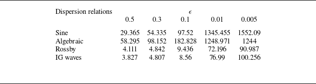Averaging these two gives us a time scale $\tau _{nl}$ and table 2 presents the ratio $\tau _{nl}/\tau _{l}$ for TV1 models for $k=10$ , this being a wavenumber in the inviscid inertial range for all regimes, as seen from the flux plots in figure 5 for example. More specific details about estimating the nonlinear time scale is given in supplementary material § 2.

Table 2.

Nonlinear to linear time scale ratio, $\tau _{nl}/\tau _{l}$ , for $k=10$ .

From table 2, we see that the ratio increases as we reduce $\epsilon$ , indicating that the nonlinear time scale is increasing with weaker nonlinearity. For all cases, we see close to an order of magnitude jump in the time scale ratio as we go from $\epsilon =0.1$ to $\epsilon =0.01$ . Substantially less change is seen with further drop in nonlinear strength, to $\epsilon =0.005$ , with the algebraic case showing an decrease of 0.3 %. These estimates, along with the linear wave energy fraction seen earlier, indicate that WWT is being attained as we reduce $\epsilon$ , with $\epsilon =0.01$ and below being regimes where nonlinear interactions are quite weak and linear wave dynamics dominate.

7. Mode-to-mode energy transfers

We will now look at the mode-to-mode or scale-to-scale energy transfers for different models as the flow transitions from the strongly nonlinear regime to weakly nonlinear regime. We define a variable at a specific mode ‘ $k$ ’ as $u_k = \hat {u}_k e^{ikx} + cc$ , where $cc$ stands for complex conjugate. This allows us to construct the whole variable as $u = \sum _k u_k$ .

To derive energy equation corresponding to mode $k$ , we first multiply (2.1) by $[u_k\ v_k]^T$ . The resulting coupled equations are then added together and integrated over the domain $[0, 2\pi ]$ . Simplifying the equation so obtained with steps detailed in the supplementary material gives us

(7.1) \begin{equation} \frac {{\rm d}E_k}{{\rm d}t} = \sum _p {T}_{k|p} \textit {,} \end{equation}

where $T_{k|p}$ is the energy transfer rate from mode $p$ to $k$ . The transfers from $p \to k$ should be equal in magnitude but opposite in sign to the transfers from $k \to p$ , i.e. $T_{k|p} = - T_{p|k}$ . This gives us $T_{k|k}=0$ , i.e. the diagonal entries of $T_{k|p}$ matrix are zero. Mode-to-mode energy transfer functions of the above form has been constructed and analysed in a broad set of past studies (Alexakis, Mininni & Pouquet Reference Alexakis, Mininni and Pouquet2005; Favier, Silvers & Proctor Reference Favier, Silvers and Proctor2014; Reun, Favier & Bars Reference Reun, Favier and Bars2021; McKeown et al. Reference McKeown, Pumir, Rubinstein, Brenner and Ostilla-Mónico2023).

Whether a turbulent downscale energy transfer is between local or non-local modes can be understood from $T_{k|p}$ . If the dominant transfers involve $p$ and $k$ such that $p/k \sim 1$ , the energy transfers are scale-local (Brasseur & Wei Reference Brasseur and Wei1994; Lesieur Reference Lesieur2008; Favier et al. Reference Favier, Silvers and Proctor2014), i.e. the transfers involve neighbouring modes or near-diagonal entries of the $T_{k|p}$ matrix. For example, HIT and dispersive waves in rotating shallow-water exhibit scale-local downscale energy transfers (Domaradzki & Rogallo Reference Domaradzki and Rogallo1990; Domaradzki & Carati Reference Domaradzki and Carati2007; Cardesa, Vela-Martin & Jimenez Reference Cardesa, Vela-Martin and Jimenez2017; Thomas et al. Reference Thomas, Rajpoot and Gupta2024). Alternatively, if dominant transfers between $p$ and $k$ are such that $p/k \gg 1$ or $k/p \gg 1$ , the transfers are non-local, involving modes that are far apart.

Recall from the energy spectra in figure 7 that the inertial range ends at $k \approx 10^3$ , beyond which dissipation range takes over. We therefore calculated $T_{k|p}$ with $n=10^3$ as the maximum wavenumber, with an emphasis on transfers in the inertial range. On calculating $T_{k|p}$ with the dissipation range included, no noticeable differences were observed and therefore, here, we will only present $T_{k|p}$ with inertial range wavenumbers.

To visualise the transfer matrix, we first time-averaged to get $\bar {T}_{k|p}$ and then normalised using a reference measure $T_{\textit{ref}}$ as $\tilde {T}_{k|p} = \bar {T}_{k|p} / T_{\textit{ref}}$ , where

(7.2) \begin{equation} T_{\textit{ref}} = \frac {1}{n} \left [ \sum _{i=1}^{n} \left | \left ( \bar {T}_{k|p} \right )_{i-1,i} \right | \right ], \end{equation}

with $(i-1,i)$ representing mode pairs just above the diagonal of the $\bar {T}_{k|p}$ and $ n = 1000$ is the number of modes considered for averaging. This normalisation helps us compare the transfer matrix across different nonlinear regimes.

Figure 10.

(a)–(e) Transition in $ \tilde {T}_{k|p}$ as $ \epsilon$ decreases in the Sine-TV1 model. The $k$ -band highlighted with grey color in panel (e) corresponds to the same band highlighted in figure 7(a). (f) Overlay of $ \tilde {T}_{k|p}$ for $\epsilon = 0.005$ and resonant modes corresponding to a tolerance of $\delta = 0.1$ , the latter being indicated by the light green coloured pattern.

Figure 11.

(a)–(e) Transition in $ \tilde {T}_{k|p}$ as $ \epsilon$ decreases in the Algebraic-TV1 model. The $k$ -band highlighted with grey color in panel (e) corresponds to the same band highlighted in figure 7(c). (f) Overlay of $ \tilde {T}_{k|p}$ for $\epsilon = 0.005$ and resonant modes corresponding to a tolerance of $\delta = 0.1$ , the latter being indicated by the light green coloured pattern.

Figure 12.

(a)–(e) Transition in $ \tilde {T}_{k|p}$ as $ \epsilon$ decreases in the Rossby-TV1 model. The $k$ -band highlighted with grey color in panel (e) corresponds to the same band highlighted in figure 7(e). (f) Overlay of $ \tilde {T}_{k|p}$ for $\epsilon = 0.005$ and resonant modes corresponding to a tolerance of $\delta = 0.1$ , the latter being indicated by the light green coloured pattern.

Figure 13.

(a)–(e) Transition in $ \tilde {T}_{k|p}$ as $ \epsilon$ decreases in the IG wave-TV1 model. The $k$ -band highlighted with grey color in panel (e) corresponds to the same band highlighted in figure 7(g). (f) Overlay of $ \tilde {T}_{k|p}$ for $\epsilon = 0.005$ and resonant modes corresponding to a tolerance of $\delta = 0.1$ , the latter being indicated by the light green coloured pattern.

Figure 10(a–e) shows the transition of $\tilde {T}_{k|p}$ for the Sine-TV1 model as $\epsilon$ decreases from $0.5$ to $0.005$ . The negative and positive transfers are shown in blue and red colour, respectively. Although we calculated transfers for up to wavenumber 1000 and this was used for subsequent analysis, for better visualisation here, we show $\tilde {T}_{k|p}$ for the range $k,p \leqslant 250$ . For $k,p \gt 250$ , the features were qualitatively similar, although the transfer magnitudes decay with increasing wavenumbers. For all $\epsilon$ cases, $\tilde {T}_{k|p}$ shows a dominant blue colour to the left of the diagonal and red colour to the right of the diagonal. This emphasises that wavenumbers $k\lt p$ are losing energy to wavenumbers $k\gt p$ , i.e. a forward energy cascade is taking place, as expected based on the energy fluxes seen before. We also see that the $k=0$ and $p=0$ regions are of higher intensity. Since the zero wavenumbers are trivially resonant with other modes, these modes are active in energy transfers. High transfer along the $k=0$ and $p=0$ regions is a feature that will be seen in all cases later, similar to the findings from several previous studies that have explored scale-to-scale transfers (Alexakis et al. Reference Alexakis, Mininni and Pouquet2005; Favier et al. Reference Favier, Silvers and Proctor2014; Reun et al. Reference Reun, Favier and Bars2021; McKeown et al. Reference McKeown, Pumir, Rubinstein, Brenner and Ostilla-Mónico2023).

For $\epsilon = 0.5$ , we see that $\tilde {T}_{k|p}$ in figure 10(a) shows high-intensity colours along near-diagonal elements, indicating scale-local transfer. However, as $\epsilon$ decreases, $\tilde {T}_{k|p}$ shows the formation of high-intensity regions that are scattered and far from the diagonal, as seen in figures 10(b) and 10(c), implying that the transfers now involve non-local modes. Observe the low intensity background modes, resembling a grid type pattern in figure 10(a), gradually getting illuminated as $\epsilon$ decreases in panels (b) and (c). Along side this, near-diagonal transfer magnitudes are getting diminished. Ultimately, a clear gridded pattern emerges in the lowest nonlinearity cases, $\epsilon = 0.01$ and $0.005$ in panels (d) and (e).

Remarkably, the resulting pattern in $\tilde {T}_{k|p}$ for the lowest $\epsilon$ cases closely resembles the pattern of the resonant modes seen in figure 3(a). To visualise this better, in figure 10(f), the resonant pattern is shown in light green colour for a tolerance $\delta = 0.1$ , as in figure 3(a), this being plotted on top of $\tilde {T}_{k|p}$ corresponding to $\epsilon = 0.005$ , i.e. the transfer function seen in figure 10(e). This comparison reveals that at the lowest $\epsilon$ values, resonant modes predominantly facilitate downscale energy transfers, the energy cascade approaching that expected in the WWT regime based on resonant modes’ interactions.

As discussed in $\S$ 2.3, the Sine dispersion relation for $\delta = 0.1$ consists of near-resonant modes surrounding exact resonant modes, forming clusters. Similar cluster patterns are seen in $\tilde {T}_{k|p}$ in figure 10(f), indicating that transfers use both exact and near-resonant modes. It is also noteworthy that some of the exact-resonant modes, such as those green lines connecting resonant clusters seen in figure 10(f), have $\tilde {T}_{k|p} \approx 0$ . Therefore, not all resonant modes are significant for downscale energy transfers.

Recall that when we examined energy spectra earlier, we saw the spectra to be developing oscillations with decreasing $\epsilon$ . On comparing $\tilde {T}_{k|p}$ and energy spectra, we found that the wavenumber bands where energy spectra peaked corresponded to high-transfer regions in $\tilde {T}_{k|p}$ , while dips in the energy spectra corresponded to low-intensity regions in $\tilde {T}_{k|p}$ . To make this comparison easier, we have highlighted an example $k$ -band, $15 \leqslant k \leqslant 25$ , highlighted with grey colour in figure 10(e). The same band is highlighted in the energy spectrum, figure 7(a). Notice that this band consists of high-intensity regions in $\tilde {T}_{k|p}$ , with resonant clusters in it. This band also peaks in the energy spectrum. On cross-comparisons, the reader will find that other peaks in the spectra also correspond to high-transfer regions in $\tilde {T}_{k|p}$ . Therefore, the oscillatory pattern we see in the spectra is a result of localised intense energy transferring modes in $\tilde {T}_{k|p}$ .

Figure 11 shows the transition of $\tilde {T}_{k|p}$ for the Algebraic-TV1 model as $\epsilon$ decreases. Recall from the second row of figure 3 that exact resonant modes are located along the near-diagonal for the algebraic dispersion relationship. Due to this, we see that scale-local energy transfers persist as $\epsilon$ reduces for this case, as seen in figure 11(a–e). Panel (f) overlays the resonant modes in light green over $\tilde {T}_{k|p}$ for $\delta =0.1$ : a feature seen here is that in addition to the resonant modes along the near-diagonal, patches of non-resonant modes are seen on either side of the diagonal. Recall that amongst all the models, the Algebraic case has the least number of resonant points. With fewer resonant modes to make the downscale transfer, the model seems to rely on non-resonant modes in addition to resonant modes to cascade energy to dissipative scales in the WWT regime with low $\epsilon$ .

We highlighted the $k$ -band $25 \leqslant k \leqslant 60$ with grey colour in figure 11(e); this band containing the significant energy transferring cluster. The same $k$ -band in the energy spectrum, also marked with grey colour in figure 7(c), shows a pronounced peak. Therefore, similar to that seen in the Sine-TV1 model, peaks in the energy spectrum at low $\epsilon$ correspond to high energy transferring mode clusters in $\tilde {T}_{k|p}$ .

The energy transfer function’s transition from strongly scale-local to weakly nonlinear resonance dominated regime for the Rossby dispersion relation is shown in figure 12. As $\epsilon$ decreases, the mode-to-mode energy transfer patterns evolve into distinct patches or clusters distributed across the $k{-}p$ space. These clusters are clearly visible in figure 12(d) for $\epsilon = 0.01$ . However, for $\epsilon = 0.005$ , the colour contrast of these clusters is significantly diminished due to the rapid decay of $\tilde {T}_{k|p}$ magnitudes at higher wavenumbers, resulting in a more subtle appearance in figure 12(e). For clarity, we have highlighted the positions of the two clusters using dashed ellipses in both figures 12(d) and 12(e). In figure 12(f), we have coloured in light green the near-resonant space corresponding to $\delta = 0.1$ , this being the same region seen in figure 3(g). Figure 12(f) shows the near-resonant region overlaid with the $\tilde {T}_{k|p}$ for $\epsilon =0.005$ . Observe that the clusters of high energy transfer regions are part of the near-resonant region.

Recall that the Rossby dispersion relation does not generate exact resonances. Yet, the Rossby-TV1 model enables energy transfer downscale through near-resonant interactions. Additionally, some of the near-resonant modes form clusters and transfer a high amount of energy, while a major fraction of the near-resonant modes remain idle. We also see that the $k$ -band $50 \leqslant k \leqslant 80$ where these clusters appear, marked as the grey region in figure 12(e), also coincides with the oscillatory peak in the energy spectrum, figure 7(e). Although not highlighted, other wavenumber bands where the energetic clusters are seen in $\tilde {T}_{k|p}$ also correspond to the peaks in the energy spectra.

Turning to the IG wave-TV1 model, figure 13 presents the mode-to-mode energy transfers for decreasing $\epsilon$ . At higher $\epsilon$ , the energy transfers are strongly scale-local, predominantly occurring along near-diagonal interactions. This scale-local behaviour persists even at lower $\epsilon$ , due to the presence of resonant modes that lie close to the diagonal, resembling the pattern observed in the Algebraic-TV1 model. However, the resonant modes for the IG wave dispersion relation are near-resonant in nature compared with the exact-resonant modes of the Algebraic model. At lower $\epsilon$ , non-resonant clusters emerge, as seen in figure 13(d,e). Similar to the Algebraic model, the IG wave model also has fewer near-resonant modes. As a result, in the WWT regime the model relies on near- and some non-resonant modes to make downscale energy transfer. As before, we also highlighted in grey the $k$ -band $25 \leqslant k \leqslant 62$ in figure 13(e), which corresponds to the region where the non-resonant cluster appears. This matches the same $k$ -band in the energy spectrum shown in figure 7(g) where a peak is observed, similar to the previous findings.

In the above discussions, we focused primarily on the TV1 model. The TV2 model results for mode-to-mode transfers were found to closely resemble those in the TV1 models despite differences in the nonlinear terms. These results are given in supplementary material § 4.

A consistent feature seen in the above-mentioned $\tilde {T}_{k|p}$ patterns is that the number of energy transferring modes decreases as we reduce $\epsilon$ . While the highest nonlinear case with $\epsilon =0.5$ was seen to have local transfers, $\tilde {T}_{k|p}$ still showed reasonably bright regions that were broadly spread. Lowering $\epsilon$ was seen to reduce such bright regions with resonant and some sparse non-resonant modes remaining at the lowest $\epsilon$ . To quantify the number of modes actively participating in the energy transfer out of the total $N_T = n^2$ modes, we define active modes $N_a$ as those whose contribution to the energy transfer is at least $10\,\%$ of $T_{\textit{ref}}$ , calculated using (7.2). That is, an active mode satisfies $\vert \tilde {T}_{k|p} \vert \geqslant 0.1$ and figure 14 shows the fraction of active mode pairs, $N_a / N_T$ versus $\epsilon$ . We see that this fraction decreases significantly for both TV1 and TV2 models as the nonlinearity weakens across all dispersion relations, as we qualitatively expected. An outlier is the Sine case as $\epsilon$ drops from 0.5 to 0.3. In this case, as seen from figure 10(a), for the highest nonlinear case of $\epsilon =0.5$ , the dominant energy transferring modes are predominantly local and are located along the near-diagonal. For $\epsilon =0.3$ , we see more resonant modes getting illuminated in figure 10(b), leading to an increase in the modes actively participating in energy transfers. A further drop in $\epsilon$ reduces the active modes for the Sine case, as seen in figure 14. With the drop in active modes with $\epsilon$ , the downscale energy transfers becomes less efficient and this leads to the system accumulating more energy at lower $\epsilon$ , as seen in figure 5(a,b).

Figure 14.

(a) and (b) Variation in the fraction of active modes ( $N_a / N_T$ ) involved in the mode-to-mode energy transfer as a function of $\epsilon$ for the TV1 and TV2 models, respectively.

The above comparison of energy transfers was made for the same dispersion case with varying $\epsilon$ , although similar comparisons can be made across models. From the $\tilde {T}_{k|p}$ plots in figures 10–13, especially at lowest $\epsilon$ value corresponding to WWT, we see that the number of dominant energy transferring modes decreases in the order: Sine $\gt$ Rossby $\gt$ IG wave $\gt$ Algebraic. The Sine dispersion relationship therefore has the most number of modes facilitating downscale transfers, while Algebraic has the least. Notice that this ordering is same as that for the number of resonant modes in different models discussed in connection to figures 2 and 3. Also recall the energy levels in different models increased as Sine $\lt$ Rossby $\lt$ IG wave $\lt$ Algebraic, as seen in figure 5(a,b). A higher number of energy transferring modes means that the system can more readily transfer energy downscale efficiently and dissipate at small scales, thereby preventing much energy accumulating in the system. The Algebraic case has the least energy transferring modes and, therefore, the system ends up gaining a lot more energy before dissipating, while the opposite is true for the Sine case. Therefore, a higher number of energy transferring modes results in a lower energy level of the system at steady state.

We conclude the discussion of mode-to-mode energy transfers by making a few common observations regarding the different models. Recall that we started at $\epsilon =0.5$ and lowered it to $\epsilon =0.005$ . Flows with $\epsilon$ higher than $0.5$ were seen to be qualitatively similar to $\epsilon =0.5$ flows, characterised by strongly nonlinear turbulence with scale-local transfers and far from the WWT regime. In some sense, these regimes are like HIT in the 3-D Navier–Stokes equation. Gradually decreasing $\epsilon$ , we found that resonance-dominated transfers started taking over for $\epsilon \leqslant 0.01$ cases across all dispersive models, as illustrated in figures 10–13. Therefore, WWT was achieved for $\epsilon \leqslant 0.01$ . In this regime, we found that exact, near- and some non-resonant transfers remained at low- $\epsilon$ values. Energy transfers were inefficient in this regime, leading to flow energy increasing with low- $\epsilon$ values. The inefficient downscale energy transfers also made it difficult to attain these WWT regimes in forced-dissipative settings. To give an example, achieving a forced-dissipative equilibrium for the Algebraic model at $\epsilon = 0.005$ required approximately four months of computation on an NVIDIA A100 GPU. With WWT achieved well enough by $\epsilon = 0.005$ and given that we had difficulty in getting flows to equilibrate for $\epsilon \lt 0.005$ even after half a year of numerical integrations, in this study, we kept the lowest value of $\epsilon$ to 0.005.

8. Intermittency

In the previous sections, we explored time-averaged energy transfers, spectra, flux and so on to understand ‘on-average’ features of the flow. Turbulent flows’ dynamics however fluctuate stochastically in space and time, specifically in wave turbulent flows, as seen in several previous studies (Falcon, Fauve & Laroche Reference Falcon, Fauve and Laroche2007a ;Reference Falcon, Laroche and Fauve b , Reference Falcon, Aumaître, Falcón, Laroche and Fauve2008; Falcon & Mordant Reference Falcon and Mordant2022). In this section, we will explore temporal intermittent features of the flows discussed earlier and examine their signatures in physical space structures.

Conventionally, intermittency in turbulence is assessed through the statistical behaviour of velocity structure functions. We use the velocity structure function

(8.1) \begin{equation} \delta _{\tau } u = u(t+\tau ) - u(t), \end{equation}

which represents the velocity increment between two points separated by a time interval ( $\tau$ ). For simplicity, we have omitted the $x$ dependence, although the increment is calculated at the same spatial point. We computed the velocity increment using many spatial points for $\tau \in \{ \delta t, 200 \delta t \}$ , with $\delta t = 10^{-3}$ . These datasets were then used to construct probability density functions (PDFs) of $\delta _{\tau } u$ for $\tau \in \{ \delta t, 200 \delta t \}$ , corresponding to the smallest and largest temporal scale separations, respectively. Two such PDFs for the Sine dispersion case for the strongest and weakest nonlinear interaction regimes are shown in figure 15. In both nonlinear strength cases, we see that the distributions match that of a Gaussian for the highest $\tau$ . However, the tails of the distributions are much fatter with significant departure from Gaussian for the lowest $\tau$ . The velocity structure function distributions therefore change depending on $\tau$ , approaching a Gaussian for large $\tau$ and deviating a lot from Gaussian for low $\tau$ . This changing behaviour of the distributions with $\tau$ characterises intermittency of the flow. Although we show only the Sine dispersion model’s result here, all other dispersion models exhibited intermittency. Consequently, all the flow regimes we are dealing with are intermittent in nature.

Figure 15.

PDF of velocity structure-functions of the variable $u$ , normalised by their standard deviations, for the Sine-TV1 model. The data are sampled at a temporal resolution ( $\delta t = 10^{-3}$ ): (a) $\epsilon = 0.5$ and (b) $\epsilon =0.005$ flow regimes.

Figure 16.

Temporal evolution of spectral flux ( $\tilde {\hat {\varPi }}_k$ , black) for $k = 10$ and dissipation ( $\tilde {D}$ , red) for varying $\epsilon$ in TV1 models: (a–e) Sine; (f–j) Algebraic dispersion relations. (k–o) Rossby; and (p–t) IG wave dispersion relations.

We will now further look at the temporal intermittent nature of the flows, and examine their features in physical space and spectral space. Figure 16 shows the time series of the spectral flux at a specific wavenumber, $k=10$ , in black colour and dissipation in red colour for the TV1 model. Other wavenumber flux time series showed similar features as described later. We picked $k=10$ , as before for the time scale computation, since this wavenumber was in the inertial range for all $\epsilon$ cases, as seen from figure 5(c,d). Figure 16(a)–(e) shows the Sine dispersion case, with $\epsilon$ dropping from 0.5 to 0.005. Similarly, panels (f)–(j) show the Algebraic case, panels (k)–(o) show the Rossby case and panels (p)–(t) show the IG wave case. TV2 models showed similar results and these are given in supplementary material § 5.

The energy flux described previously is in spectral space while dissipation is in physical space. For combined plots of flux and dissipation, we normalised both variables with respect to their time-averaged values. Specifically, we define the normalised flux as $\tilde {\hat {\varPi }}_k = \hat {\varPi }_k (k = 10) / \bar {\hat {\varPi }}_k (k = 10)$ and the normalised dissipation as $\tilde {D} = D / \bar {D}$ , where overbar denotes time average. The normalised time series of $\tilde {\hat {\varPi }}_k$ and $\tilde {D}$ are shown in black and red curves, respectively, in figure 16.

Looking at figure 16(a) for the Sine case with $\epsilon =0.5$ , we see that the energy flux and dissipation exhibit significant fluctuations, with each of them showing high-value jumps at specific time instances, which we will call ‘bursts’. Such bursts with flow variables, such as dissipation, exhibiting extreme values for a small time window, have been commonly observed in HIT, rotating and stratified turbulent flows (Frisch & Morf Reference Frisch and Morf1981; Read et al. Reference Read, Collins, Früh, Lewis and Lovegrove1998; Rorai, Mininni & Pouquet Reference Rorai, Mininni and Pouquet2014; Yeung, Zhai & Sreenivasan Reference Yeung, Zhai and Sreenivasan2015; Carter & Coletti Reference Carter and Coletti2018; Elsinga, Ishihara & Hunt Reference Elsinga, Ishihara and Hunt2020; Marino et al. Reference Marino, Feraco, Primavera, Pumir, Pouquet, Rosenberg and Mininni2022; Thomas et al. Reference Thomas, Rajpoot and Gupta2024). In our case, we see that reducing $\epsilon$ makes the bursts rarer with a longer gap between successive bursts. In figure 16(a)–(c), we chose a time interval of $100$ , starting from an arbitrary time $t_1$ . For panels (d) and (e), we however chose a longer time interval of 1000, since the bursts were much rarer. Similar time intervals are shown for the Rossby and IG wave-TV1 models in figures 16(k–o) and 16(p–t), respectively. For the Algebraic model, however, a much longer interval $\Delta t = 10^4$ is shown in figure 16(i,j) for the lowest nonlinearity cases ( $\epsilon = 0.01$ and $0.005$ ) since the bursts were much rarer in these regimes of the model. These results indicate that turbulent transfers become more intermittent in time as we approach the WWT regime.

Comparing flux and dissipation, we see that the two fields appear to be synchronised. However, on a careful examination, we could find a small time delay between the two, with dissipation peaking after flux. This is highlighted by the inset in figure 16(c). Since it takes a non-zero amount of time for energy to cascade across the inertial range to reach dissipative scales, a time lag is expected between energy flux and dissipation. A similar time lag has been reported in previous studies on HIT and rotating shallow water flows (Cardesa et al. Reference Cardesa, Vela-Martín, Dong and Jiménez2015; Khurshid, Donzis & Sreenivasan Reference Khurshid, Donzis and Sreenivasan2021; Thomas et al. Reference Thomas, Rajpoot and Gupta2024).

We also found that the amplitudes of the bursts for weakly nonlinearity cases ( $\epsilon = 0.01 \text{ and } 0.005$ ) were relatively larger than that of strong nonlinearity cases ( $\epsilon = 0.5, 0.3 \text{ and } 0.1$ ). For example, $\tilde {\hat {\varPi }}_k$ maxima for the Algebraic case in figures 16(i) and 16(j) are ${\sim}\, 600$ and $1500$ , whereas the corresponding values in figures 16(f), 16(g) and 16(h) are ${\sim}\, 6, 15$ and $30$ , respectively. Qualitatively similar trends were seen for other models as well. This behaviour follows from the fact that all the flows were forced with the same energy injection rate, leading to the same on-average energy dissipation. Flux and dissipation bursts correspond to time instants when there is a higher contribution towards averaged flux and dissipation than other time instances. Therefore, with the bursts becoming rarer at lower $\epsilon$ , the flux and dissipation burst event amplitudes have to be much higher to generate the same averaged dissipation as in higher $\epsilon$ cases.

Taking a closer look at the flux time series, we see that the instantaneous flux can be positive or negative, even though the averaged flux is positive, inducing a forward cascade. From the flux time series, we see that all dispersive models for higher nonlinearity cases ( $\epsilon = 0.5, 0.3 \text{ and } 0.1$ ) have quite low magnitudes of negative $\tilde {\hat {\varPi }}_k$ compared with the positive counterparts. This can be seen by comparing positive and negative flux maxima in panels (a)–(c), (f)–(h), (k)–(m) and (p)–(r) of figure 16. However, as $\epsilon$ reduces to 0.01 and 0.005, the amplitudes of negative fluxes increases. This feature is much more pronounced in the Algebraic-TV1 model: see figures 16(i) and 16(j). For the $\epsilon = 0.005$ case, the maximum magnitude of negative flux becomes comparable to that of the positive one in the TV1 model (figure 16 j) and even surpasses that in the TV2 model (supplementary material figure S5j).

When amplitudes of negative flux become comparable to that of positive flux bursts, the forward energy cascade becomes much more inefficient with the flow taking much longer to dissipate energy. This is why the integration for the Algebraic model with $\epsilon = 0.01$ and $0.005$ required four months of computational time, as mentioned earlier. This inefficiency in downscale cascade and extremely long time needed for the system to dissipate energy is reminiscent of the ‘frozen turbulence’ regime described by Pushkarev & Zakharov (Reference Pushkarev and Zakharov2000). In this regime, several localised clusters of modes at low wavenumbers exchange energy among themselves without cascading energy to dissipative scales. The algebraic model seems to be on its path to frozen turbulence, since long-time integrations of the model with $\epsilon$ below 0.005 that we attempted did not reach equilibrium even after 6 months of integration, due to insignificant small-scale dissipation.

Oscillatory spectra arising from discreteness (finite-size) effects under weak nonlinearity are often considered as a signature of frozen turbulence. However, the presence of spectral oscillations alone is not a sufficient indicator of frozen turbulence. A defining feature of frozen turbulence is a substantial negative spectral flux, with a magnitude comparable to or exceeding the positive flux. Our flux time series shows that although oscillatory spectra are observed for the Sine dispersion relation (and others), the negative flux remains negligible and the system reaches a statistically steady state, thereby ruling out frozen turbulence. In contrast, the Algebraic dispersion relation exhibits a significant negative flux despite the absence of strong spectral oscillations. Nevertheless, since the system still evolves towards a steady state, this regime cannot be regarded as fully frozen; rather, it can be considered close to frozen turbulence. These results demonstrate that frozen turbulence is more reliably characterised by flux behaviour than by spectral oscillations alone.

Comparing the burst events across $\epsilon$ , we see that bursts in figure 16(a) are not only frequent, but also sharp and isolated, each characterised by rapid onset and decay. In contrast, figure 16(e) shows less frequent, but broader bursts, with each event comprising a gradual increase and decrease. This is a characteristic feature in all dispersive models as $\epsilon$ decreases and can be seen in figure 16. We calculated the number of burst-events per unit time interval as a function of $\epsilon$ from the dissipation ( $\tilde {D}$ ) time series to quantify the intermittency. For this, we used the interquartile range ( $IQR$ ) method for identifying bursts (Fischer, Schaar & Theis Reference Fischer, Schaar and Theis2023; Erhart et al. Reference Erhart, Yoshida, Khinevich and Mizukami2024; Han, Pei & Tong Reference Han, Pei and Tong2024). It is a method for outlier detection in which $IQR = Q_3 - Q_1$ represents the range of data that lies between the first quartile ( $Q_1$ ) and the third quartile ( $Q_3$ ). Specifically, $Q_1$ and $Q_3$ are the medians corresponding to the smallest and largest $50\,\%$ amplitudes of the time series, respectively. Consequently, a cutoff is set as $\gamma = Q_3 + 1.5 \times IQR$ . That is, a dissipation burst is considered to have taken place if $\tilde {D} \gt \gamma _D$ , where $\gamma _D$ is the cutoff as obtained from $\tilde {D}$ time series.

As seen previously, burst events are spread wider in time at lower $\epsilon$ . Once a burst was identified using the above-mentioned procedure at a particular time $t_0$ , we isolated this burst event such that no new burst event gets counted in the small time interval $(t_0-5 \delta t, t_0+5\delta _t)$ , $\delta t$ being the time increment associated with the high resolution time series. This procedure prevented multiple counting of a particular burst event. An illustration of the $IQR$ method with specific details is given in supplementary figure S6.

Figure 17.

(a) and (b) Variation in the burst-events per unit time ( $N_b$ ) as a function of $\epsilon$ , calculated from the dissipation time series using the $IQR$ method, for TV1 and TV2 models.

Following the IQR method, figures 17(a) and 17(b) shows the variation in the number of burst-events per unit time ( $N_b$ ) as a function of $\epsilon$ for both TV1 and TV2 dispersive models, respectively. Although there are exceptions at higher $\epsilon$ , in general, we see that $N_b$ decreases as $\epsilon$ decreases, as anticipated based on the time series of dissipation and flux for different models earlier. WWT is therefore highly intermittent in nature with a drop in forward cascading and dissipation efficiency.

9. Coherent structures and their dynamics

The burst events noted above are associated with distinct coherent physical structures in the flow. Such features were seen to be specifically prominent in the WWT regime with $\epsilon \leqslant 0.01$ , while we did not find distinctly noteworthy features accompanying burst events in physical space for the $\epsilon \geqslant 0.01$ cases. Here, we will present results for $\epsilon = 0.005$ for the different dispersive models.

Figure 18.

(a) Dissipation time series, $\tilde {D}(t)$ , of Sine-TV1 model at $\epsilon = 0.005$ . Physical structure of $u$ and $v$ during two distinct burst-events, identified by cyan-coloured points: $\{P_1, P_2, P_3\}$ and $\{P_4, P_5, P_6\}$ in panel (a), are shown in two columns: panels (b)–(d) and (e)–(f) below panel (a). Panels (h) and (i) show the energy spectra associated with the first and second burst-events, respectively.

Figure 19.

(a) Dissipation time series, $\tilde {D}(t)$ , of Algebraic-TV1 model at $\epsilon = 0.005$ . Physical structure of $u$ and $v$ during two distinct burst-events, identified by cyan-coloured points: $\{P_1, P_2, P_3\}$ and $\{P_4, P_5, P_6\}$ in panel (a), are shown in two columns: panels (b)–(d) and (e)–(f) below panel (a). Panels (h) and (i) show the energy spectra associated with the first and second burst-events, respectively.

Figure 20.

(a) Dissipation time series, $\tilde {D}(t)$ , of Rossby-TV1 model at $\epsilon = 0.005$ . Physical structure of $u$ and $v$ during two distinct burst-events, identified by cyan-coloured points: $\{P_1, P_2, P_3\}$ and $\{P_4, P_5, P_6\}$ in panel (a), are shown in two columns: panels (b)–(d) and (e)–(f) below panel (a). Panels (h) and (i) show the energy spectra associated with the first and second burst-events, respectively.

Figure 21.

(a) Dissipation time series, $\tilde {D}(t)$ , of IG wave-TV1 model at $\epsilon = 0.005$ . Physical structure of $u$ and $v$ during two distinct burst-events, identified by cyan-coloured points: $\{P_1, P_2, P_3\}$ and $\{P_4, P_5, P_6\}$ in panel (a), are shown in two columns: panels (b)–(d) and (e)–(f) below panel (a). Panels (h) and (i) show the energy spectra associated with the first and second burst-events, respectively.

Figure 22.

Comparison of the spectral flux and energy spectrum during intermittent burst events and non-burst (quiescent) periods. Panel (a) identifies burst events (shaded in grey). Panel (b) compares the spectral flux averaged over burst events with that averaged over non-burst periods, while panel (c) shows their respective contributions to the total flux. Panels (d) and (e) present the corresponding comparisons of the averaged energy spectra and their contributions, respectively. Note that the green curve overlaps a lot with the red curve in panel (e).

Figure 18(a) shows the dissipation time series for $\epsilon = 0.005$ in the Sine-TV1 model, this being the same curve from figure 16(e). On this time series, we have marked six time instances ( $P_1, P_2, \ldots ,P_6$ ) using cyan-filled circles. These markers highlight two distinct burst-events, each represented by a triplet of points: one preceding the onset, one at the peak and one following the decay of the burst-event. Specifically, $\{P_1, P_2, P_3\}$ and $\{P_4, P_5, P_6\}$ correspond to the first and second burst-events, respectively. The corresponding physical structure of $u$ and $v$ are shown below panel (a) in two columns: the first column with panels (b)–(d) for $\{P_1, P_2, P_3\}$ and the second column with panels (e)–(g) for $\{P_4, P_5, P_6\}$ . Additionally, the energy spectra at these specific instances are shown in the bottom row of the figure with panels (h) and (i) corresponding to the first and second burst-events, respectively. A similar panel arrangement is used for the other models: figure 19 for Algebraic, figure 20 for Rossby and figure 21 for IG wave-TV1 models.

As seen in panels (c) and (f) of figure 18, high amplitude localised physical structures appear at the peak of the two burst-events, $P_2$ and $P_5$ , for the Sine-TV1 model. These structures are nearly absent during the pre- and post-burst-event times, as seen in panels (b) and (e) for $\{ P_1, P_4 \}$ and panels (d) and (g) for $\{ P_3, P_6 \}$ . Since these large amplitude localised features appear intermittently with burst-events, they may be identified as non-stationary coherent structures. For the other dispersive models, the coherent structures at burst-peaks resemble spatially localised wave packets, as seen in panels (c) and (f) of figure 19, figure 20 and figure 21 for the Algebraic-, Rossby- and IG wave-TV1 models, respectively. Just like the localised structures in the Sine-TV1 model, the wave packets are absent during the pre- and post-burst-event times, as seen from figures 19, 20 and 21. Such localised structures are often called quasi-solitons, as used by Zakharov et al. (Reference Zakharov, Dias and Pushkarev2004). Unlike true solitons, these quasi-solitons disperse and interact inelastically, as verified from the evolution of the structures we examined over a longer time window. These quasi-solitons were seen to grow and decay during each turbulent burst-event. Consequently, the lifetime of these structures corresponds to the duration of the turbulent bursts, as illustrated in figure 18 and in the analogous figures for the other models.

Let us now focus on the energy spectra corresponding to the burst-event time instances. As shown in figures 18(h) and 18(i), the spectra corresponding to $P_2$ and $P_5$ (shown in red) are much shallower with more energy at small scales than the other spectra: the blue and green spectra, which corresponds to $ \{ P_1, P_4 \}$ and $\{ P_3, P_6 \}$ , respectively, for the Sine-TV1 model. Similar behaviour was observed for other models as well: see the last row of figures 19, 20 and 21. The burst therefore generated localised high amplitude coherent structures, which in turn generated shallower energy spectra. The physical signatures associated with the TV2 models were seen to be similar to those of the TV1 models, and are shown in supplementary material figures S7–S10.

Because coherent structures are robustly observed in all weakly nonlinear regimes examined here, they can be regarded as a general feature of the dynamics. However, their presence does not imply that they are the primary drivers of energy transfer. Rather, they represent intermittent manifestations of rapid downscale energy-transfer events arising from the underlying wave–wave interactions.

To quantify the point made above, we analyse the spectral flux associated with coherent structures. Figure 22(a) highlights intermittent burst events as grey-shaded regions in the dissipation time series for $\epsilon = 0.005$ in the Sine-TV1 model (the same time series shown in figure 16 e). The spectral flux averaged over these burst time intervals alone ( $\bar {\hat {\varPi }}_b$ ) is computed and compared with the flux averaged over the remaining non-burst time intervals ( $\bar {\hat {\varPi }}_{nb}$ ) in figure 22(b). Notice that the average flux is much higher during burst events, i.e. $\bar {\hat {\varPi }}_b \gg \bar {\hat {\varPi }}_{nb}$ , as we would have expected. However, the burst events appear only for a small fraction of time. In figure 22(c), we show three fluxes. With a green line, we show the total flux averaged over the whole time window $\Delta t$ , $\bar {\hat {\varPi }}$ . Out of the total time window, $\Delta t_b$ and $\Delta t_{nb}$ are burst and non-burst time intervals such that $\Delta t_b + \Delta t_{nb} = \Delta t$ . These help us to split the averaged flux $\bar {\hat {\varPi }}$ into a contribution coming from bursts events, $(\Delta t_b / \Delta t)\bar {\hat {\varPi }}_b$ , and a contribution coming from non-burst times, $(\Delta t_{nb} / \Delta t)\bar {\hat {\varPi }}_{nb}$ , these being shown with red and blue lines in figure 22(c). By construction, the sum of these two averaged fluxes equals the total averaged flux. From the figure, we see that the averaged flux contribution from burst events is only slightly higher than the averaged flux during non-burst events. Since the bursts are intermittent and appear only for a small time window, even though they are associated with a higher flux, their contribution averaged over a longer time window becomes comparable to flux during non-burst periods averaged over the same long window.

Following similar notation as for the flux, the last row of figure 22 shows the energy spectra and its decompositions. From panel (d), we see that the red spectra averaged during bursts is shallower than the blue one averaged during non-bursts. From panel (e), we see that the averaged spectrum during burst events overlaps well with the net averaged spectrum. Therefore, burst-time spectrum is a good approximation for the total averaged spectrum. Another interesting observation from the spectra plots is that the oscillations in the spectra persist during burst and non-bursts time windows. As discussed in § 7, peaks and valleys in the spectra correspond to the modes associated with high- and low-energy transfers. These oscillations therefore remain during bursts and non-burst events.

The results were qualitatively similar for all other dispersion and nonlinear models as well, although here, in the interest of space, we presented only Sine-TV1 results. Importantly, these findings demonstrate that coherent structures are not necessary for sustaining the weakly nonlinear downscale energy cascade. Even in their absence, energy transfer from forcing to dissipation scales persists. Energy transfers in the WWT are therefore driven primarily by wave–wave interactions, with temporally intermittent relatively rare high flux events being accompanied with coherent structures in physical space.

10. Summary and discussion

Turbulent nonlinear interactions between dispersive waves is ubiquitous in many physical systems, including oceanic and atmospheric flows. Such geophysical flows are composed of several decades of spatio-temporal scales and direct numerical simulations are still far from resolving all the relevant energy containing scales in those flows. As a consequence, the detailed pathways dispersive waves take to transfer energy from large forcing scales to small dissipative scales and related questions remain largely unresolved.

Dispersive waves are associated with specific resonance conditions that dictate how wavenumbers and frequencies of the interacting waves are related. Under these conditions, if weakly nonlinear waves interact in an unbounded domain, a wave kinetic equation can be derived to characterise wave energy transfers (Zakharov, L’vov & Falkovich Reference Zakharov, L’vov and Falkovich1992; Nazarenko Reference Nazarenko2011). However, realistic flows are often set in finite domains and have varying levels of nonlinear interaction strengths. Under these conditions, do turbulent waves follow the spectral pathways dictated by resonances? At what point should we expect the weak wave turbulence (WWT) regime and energy transfers dominated by resonant interactions? Additionally, how does intermittency of energy transfers change as we move from strong turbulence to WWT?

The above-mentioned questions are key to understanding and parametrising unresolved fast wave dynamics in coarse resolution climate and forecast models. Of course, as mentioned, resolving all the relevant scales in geophysical flows is challenging at present, although insights on qualitative features of turbulent wave transfers may be understood from reduced models. With this in mind, we constructed a set of one-dimensional models of wave turbulence by using different kinds of dispersion relationships with quadratic nonlinear interaction terms. Despite being one-dimensional, as described in the earlier sections, tracking wave turbulent transfers numerically in WWT took approximately half a year with modern GPU machines.

We set up four kinds of dispersion relations in our models: (i) Sine (sinusoidal); (ii) Algebraic; (iii) Rossby (Rossby wave); and (iv) IG wave (internal gravity wave). The Sine dispersion relation was inspired by lattice vibration models (Onorato et al. Reference Onorato, Vozella, Proment and Lvov2015; Lvov & Onorato Reference Lvov and Onorato2018; Bustamante et al. Reference Bustamante, Hutchinson, Lvov and Onorato2019) and is characterised by a large number of exact resonant points. The Algebraic relation however has only a few exact resonances along specific lines. Rossby and IG wave relations were constructed with inspiration from similar named waves in geophysical flows, and has only near-resonances. Between them, Rossby has a lot more resonant points than IG waves. Along with these dispersion relations, we used two kinds of quadratic nonlinearities, constructed such that the models conserved total energy. Varying the two kinds of nonlinear terms and four kinds of dispersion relations gave us 8 models in total. We further varied the strength of the nonlinear terms, denoted by $\epsilon$ , across five values: $\epsilon \in \{ 0.5, 0.3, 0.1, 0.01, 0.005 \}$ . This gave us a total of 40 different dynamic regimes and we generated forced-dissipative equilibrated flows in these regimes to analyse the transition from the strongly nonlinear to WWT regime. Importantly, we generated all the flows by injecting energy at the same rate. As a result, all the flows had the same average energy cascade rate and dissipation rate.

On reducing $\epsilon$ from 0.5 to 0.005, we found that the flows transitioned from strongly nonlinear dynamics at high- $\epsilon$ to WWT regime for the low- $\epsilon$ values. Tracking the fraction of linear waves, we found that, in general, higher $\epsilon$ flows had only approximately 15 % energy in linear waves, while low $\epsilon$ WWT flows had most of the energy in linear waves. On examining the time series of energy flux and dissipation for the flows, we found that the WWT regime flows had dissipation and flux peaking intermittently as ‘bursts’ with longer time gaps between the bursts, while the higher $\epsilon$ strongly nonlinear flows had more frequent bursts in dissipation and flux. The bursts also had higher amplitudes in the WWT regime. Along side these bursts, we saw the formation of localised high amplitude coherent structures in the physical domain, which intermittently appeared at the burst and disappeared once the burst died off.

With the flux and dissipation bursts being more intermittent in the WWT regime, the low- $\epsilon$ flows were more inefficient in their energy dissipation. This inefficiency led to flow energy increasing as $\epsilon$ was reduced, i.e. lower $\epsilon$ flows due to their inefficient dissipation allowed their energy levels to increase. However, higher $\epsilon$ flows with their efficient dissipation did not have their energy levels increase so much. We constructed an efficiency metric that quantified the cascade efficiency of the flows reducing as $\epsilon$ reduced.

The transition from the strong turbulence to WWT regime was also characterised by steepening of the energy spectra along with oscillations in the spectra at low- $\epsilon$ values. While all the flows had similar inertial range flux, the inertial range was seen to reduce as we moved towards WWT, with a staircase-like pattern appearing in the high-wavenumber end of the flux. Prominent oscillations in energy spectra, as we found, have been reported in multiple past studies on wave turbulence in different settings (Falkovich & Shafarenko Reference Falkovich and Shafarenko1988; Pushkarev & Zakharov Reference Pushkarev and Zakharov2000; Proment et al. Reference Proment, Nazarenko and Onorato2009). Similarly, the steepening of spectra with decreasing $\epsilon$ is also consistent with findings from past studies on rotating and stratified wave turbulent flows (Bartello & Tobias Reference Bartello and Tobias2013; Rodda et al. Reference Rodda, Savaro, Bouillaut, Augier, Sommeria, Joël, Valran, Viboud and Mordant, Nicolas2023; Thomas et al. Reference Thomas, Rajpoot and Gupta2024).

Exploring the mode-to-mode energy transfers and their features as the flow transitions from strong to weak turbulence, we found that scale-local transfer, similar to HIT, dominated at high $\epsilon$ . However, low- $\epsilon$ flows in the WWT regime were characterised by resonant modes being dominant contributors of downscale energy transfers. For the Sine dispersion relation in the WWT regime, we found the energy transfers to be high at exact and near-resonant modes. The Algebraic case had high transfer values on the exact resonant lines and also some non-resonant modes. Rossby and IG wave cases had near-resonant modes contribute to the transfers. Out of these, we found IG wave, which had limited near-resonant modes, involved some non-resonant modes in the downscale transfers.

The above-mentioned results indicate that when a flow in the WWT regime has a low number of exact or near-resonant modes, it will rely on non-resonant modes to downscale cascade energy. This was the case for Algebraic and IG wave dispersion relations. Also recall the previous discussion of oscillations in the energy spectra. We found that the peaks and dips in the spectra corresponded to energy transferring cluster of modes. Higher energy transfer modes generated peaks in the spectra, while low transfer modes corresponded to dips in the spectra.

On comparing the number of modes involved in dominant energy transfers in WWT, we found the numbers to follow the order: Sine $\gt$ Rossby $\gt$ IG Wave $\gt$ Algebraic. Sine had the most, while Algebraic had the least number of dominant energy transferring modes. Interestingly, the flow energy levels in different models in WWT ordered as Sine $\lt$ Rossby $\lt$ IG Wave $\lt$ Algebraic, the opposite of dominant energy transferring modes. Therefore, a higher number of dominant energy transferring modes results in a more efficient downscale energy transfer and dissipation, this in turn lowering the flow energy.

As part of the transition to WWT, a noteworthy result is the significant steepening of energy spectra with inefficient energy cascade. Similar spectrum steepening has been seen with internal gravity waves in experiments; for example, Rodda et al. (Reference Rodda, Savaro, Bouillaut, Augier, Sommeria, Joël, Valran, Viboud and Mordant, Nicolas2023) observed a steep spectrum of $-4.5$ for weakly nonlinear internal waves. In contrast, the atmospheric and oceanic spectra are often shallower and closer to $-5/3$ or $-2$ . While it is non-trivial to directly extrapolate features of our results to fully three-dimensional cases, there exists the possibility that those geophysical spectra are not created by weakly nonlinear waves in the WWT regime. This was speculated by Holloway (Reference Holloway1980) based on ocean observations, hinting that the GM spectrum forming oceanic internal waves might not just be weak waves.

In summary, the present study provided us with several key insights on dispersive wave turbulence by comparing how different models transition from the strong turbulence to WWT regime. While resonant transfers are in general expected to dominate in the WWT regime, our findings of not all resonant modes playing equal role and near-resonant transfers being non-negligible were interesting results. Additionally, non-resonant modes participating in downscale energy transfers for models that had few resonant modes was unexpected. The extreme temporal intermittency in downscale energy transfers for different models was another notable feature of the WWT regime. These findings, in general, highlight the need to carefully consider the wave turbulence dynamics of dispersive waves in geophysical flows before developing parametrisations for coarse resolution models. Models built by using exact resonant modes alone might not capture the downscale energy transfer pathways accurately.