1 Introduction
Stratified turbulence is strongly anisotropic with predominantly horizontal motions but high shear along the vertical (Riley & Lelong Reference Riley and Lelong2000). Such layered structure inherently promotes the shear instability, which breaks down the layers into smaller-scale turbulence (Lilly Reference Lilly1983; Riley & deBruynKops Reference Riley and deBruynKops2003; Lindborg Reference Lindborg2006). This is thought to be one of the main mechanisms that accomplish the direct energy cascade towards small scales in stratified turbulence (Laval, McWilliams & Dubrulle Reference Laval, McWilliams and Dubrulle2003; Riley & deBruynKops Reference Riley and deBruynKops2003; Brethouwer et al. Reference Brethouwer, Billant, Lindborg and Chomaz2007; Deloncle, Billant & Chomaz Reference Deloncle, Billant and Chomaz2008; Augier & Billant Reference Augier and Billant2011; Augier, Chomaz & Billant Reference Augier, Chomaz and Billant2012; Waite Reference Waite2013).
In his pioneering paper on strongly stratified flows, Lilly (Reference Lilly1983) conjectured a simple mechanism for the growth of the vertical shear. He considered a uniform horizontal flow directed along a given direction, let us say  $x$, and vertically sheared:
 $\boldsymbol{U}=U(z)\boldsymbol{e}_{x}$ where
 $z$ is the vertical coordinate. If a coherent structure with initial horizontal velocity
 $\boldsymbol{u}_{h0}(x,y,z)$ is embedded within this shear flow, it will be advected differentially depending on the vertical position:
 $$\begin{eqnarray}\frac{\unicode[STIX]{x2202}\boldsymbol{u}_{h}}{\unicode[STIX]{x2202}t}=-U\frac{\unicode[STIX]{x2202}\boldsymbol{u}_{h}}{\unicode[STIX]{x2202}x}.\end{eqnarray}$$
Lilly further assumed that the coupling along the vertical is weak in the limit of strong stratification. When the vertical coupling is zero, the flow consists of a stack of horizontal two-dimensional flows evolving independently at each level  $z$. Then, the solution at any time is simply
 $\boldsymbol{u}_{h}(x,y,z,t)=\boldsymbol{u}_{h0}(x-U(z)t,y,z)$. This shows that the vertical shear should grow algebraically with time according to
 $$\begin{eqnarray}\frac{\unicode[STIX]{x2202}\boldsymbol{u}_{h}}{\unicode[STIX]{x2202}z}=-\frac{\text{d}U}{\text{d}z}t\frac{\unicode[STIX]{x2202}\boldsymbol{u}_{h0}}{\unicode[STIX]{x2202}x}+\frac{\unicode[STIX]{x2202}\boldsymbol{u}_{h0}}{\unicode[STIX]{x2202}z}.\end{eqnarray}$$
On this basis, Lilly (Reference Lilly1983) argued that the Richardson number should sooner or later reach the critical value  $1/4$ for the onset of the shear instability (Howard Reference Howard1961; Miles Reference Miles1961). However, a key assumption behind this conjecture is that there is no vertical coupling. This derives directly from Lilly’s assumption that the vertical Froude number tends to zero in the limit of strong stratification. It is now acknowledged that the vertical Froude number remains of order unity because the typical vertical length scale is the buoyancy length scale in strongly stratified flows (see, among others, Herring & Métais (Reference Herring and Métais1989), Billant & Chomaz (Reference Billant and Chomaz2000, Reference Billant and Chomaz2001), Godeferd & Staquet (Reference Godeferd and Staquet2003), Laval et al. (Reference Laval, McWilliams and Dubrulle2003), Waite & Bartello (Reference Waite and Bartello2004), Lindborg (Reference Lindborg2006)).
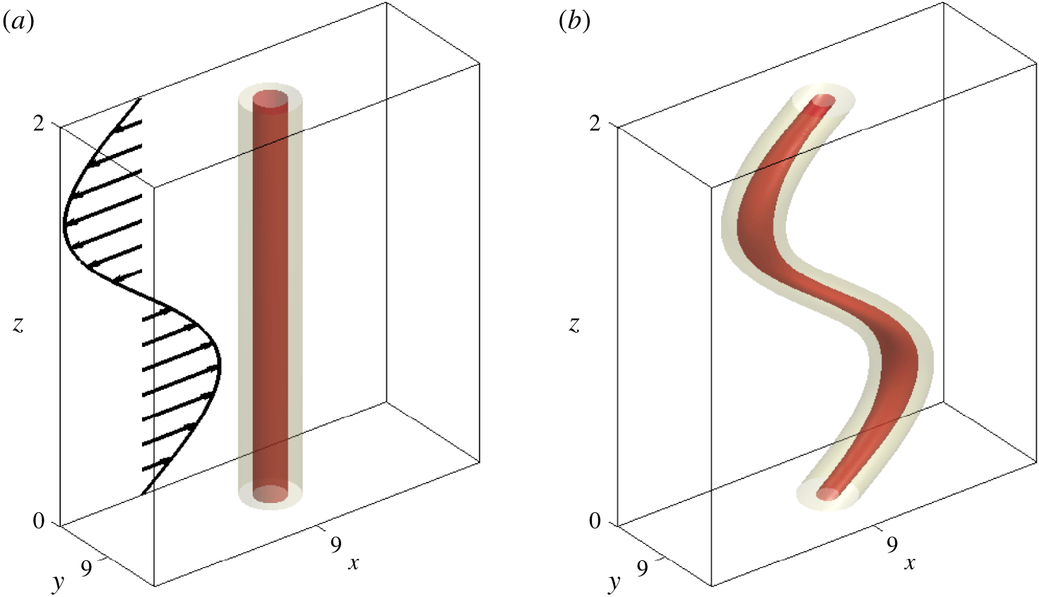
It is therefore unknown whether or not this mechanism for the growth of the vertical shear is valid. In order to answer this question, we have considered the particular case of an initially vertical vortex in an ambient vertically sheared flow in a stratified fluid. This flow configuration is sketched in figure 1 together with the example of a direct numerical simulation illustrating the vortex evolution. In the present paper, we shall study the dynamics of this flow by an asymptotic analysis while direct numerical simulations will be performed in Part 2 (Billant & Bonnici Reference Billant and Bonnici2020).
(a) Sketch of the flow configuration studied in this paper. The ambient shear flow  $U(z)\boldsymbol{e}_{x}$ is represented by the black vectors. The dark grey (red) and light grey (yellow) contours show two levels of the potential vorticity of the vortex at
 $t=0$. (b) Potential vorticity contours at
 $t=20$ obtained from a direct numerical simulation for the Froude and Reynolds numbers
 $F_{h}=0.1$,
 $Re=6000$ and the shear flow
 $U=U_{S}\sin (k_{z}z)$ with
 $U_{S}=0.2$ and
 $k_{z}=\unicode[STIX]{x03C0}$. These parameters are defined in § 2. See Billant & Bonnici (Reference Billant and Bonnici2020) for the details of the numerical simulations.

The dynamics of an isolated vortex in an ambient sheared flow has been studied before in stratified rotating fluids in order to understand the dynamics of atmospheric tropical cyclones (Jones Reference Jones1995, Reference Jones2000a,Reference Jonesb, Reference Jones2004; Sutyrin & Morel Reference Sutyrin and Morel1997; Frank & Ritchie Reference Frank and Ritchie1999; Reasor, Montgomery & Grasso Reference Reasor, Montgomery and Grasso2004; Päschke et al. Reference Päschke, Marschalik, Owinoh and Klein2012) or oceanic vortices (Vandermeirsch, Morel & Sutyrin Reference Vandermeirsch, Morel and Sutyrin2001, Reference Vandermeirsch, Morel and Sutyrin2002). In particular, Jones (Reference Jones1995), using a three-dimensional continuous hydrostatic primitive equation model, has shown that an initially barotropic vortex in a linear shear flow tilts in the shear direction but also executes a cyclonic rotation about its mid-level centre. Päschke et al. (Reference Päschke, Marschalik, Owinoh and Klein2012) have derived asymptotic equations for the motion of the vortex centre in the case of a weak shear flow.
The influence of a vertical shear on an initially aligned vortex has also been investigated by means of quasi-geostrophic two-layer models (Marshall & Parthasarathy Reference Marshall and Parthasarathy1993; DeMaria Reference DeMaria1996; Smith, Ulrich & Sneddon Reference Smith, Ulrich and Sneddon2000; Vandermeirsch et al. Reference Vandermeirsch, Morel and Sutyrin2001, Reference Vandermeirsch, Morel and Sutyrin2002). Marshall & Parthasarathy (Reference Marshall and Parthasarathy1993) have reported two distinct evolutions depending on the strength of the vortices compared to the shear. When the advection by the shear is below a critical value, the vortices in each layer are offset and rotate about each other. Conversely, when the advection is sufficiently strong, the two vortices are continuously advected away from each other. These two regimes have been called non-tearing and tearing regimes, respectively.
In contrast, the dynamics of an isolated vortex subjected to a vertical shear in stratified non-rotating fluids has been little investigated so far. Boulanger, Meunier & Le Dizès (Reference Boulanger, Meunier and Le Dizès2007, Reference Boulanger, Meunier and Le Dizès2008) have considered the dynamics of a vortex slightly tilted with respect to the direction of stratification. However, the tilt of the vortex is not created by an external shear flow but by the method of generation of the vortex. Majda & Grote (Reference Majda and Grote1997) have studied the effect of a vertically sheared mean horizontal flow on a vortex pair but only by means of the reduced equations of Lilly (Reference Lilly1983), which are valid in the limits of zero vertical and horizontal Froude numbers. Here and in Part 2 (Billant & Bonnici Reference Billant and Bonnici2020), we will study the dynamics of a Lamb–Oseen vortex in a sinusoidally sheared flow using the full Navier–Stokes equations under the Boussinesq approximation with the aim of testing Lilly’s conjecture for the growth of vertical shear.
In the present paper, an asymptotic analysis is conducted in § 3 for long vertical wavelength following a similar approach to that used by Billant (Reference Billant2010) to describe the zigzag instability of columnar vortices in stratified rotating fluids. This analysis provides the governing equations for the displacements of the vortex centre (§ 3.2.1) and the evolution of its vertical vorticity (§ 3.2.2) due to the shear flow. These equations are further analysed in §§ 4.2 and 4.1, respectively. The evolution of the Richardson number is then studied in § 4.3. These asymptotic predictions will be compared to direct numerical simulations (DNS) in Part 2.
2 Formulation of the problem
2.1 Governing equations
We consider the incompressible Navier–Stokes equations written within the Boussinesq approximation:
 $$\begin{eqnarray}\displaystyle & \displaystyle \unicode[STIX]{x1D735}\boldsymbol{\cdot }\boldsymbol{u}=0, & \displaystyle\end{eqnarray}$$
 $$\begin{eqnarray}\displaystyle & \displaystyle \frac{\unicode[STIX]{x2202}\boldsymbol{u}}{\unicode[STIX]{x2202}t}+(\boldsymbol{u}\boldsymbol{\cdot }\unicode[STIX]{x1D735})\boldsymbol{u}=-\unicode[STIX]{x1D735}\left(\frac{p}{\unicode[STIX]{x1D70C}_{0}}\right)+b\boldsymbol{e}_{z}+\unicode[STIX]{x1D708}\unicode[STIX]{x1D6FB}^{2}\boldsymbol{u}, & \displaystyle\end{eqnarray}$$
 $$\begin{eqnarray}\displaystyle & \displaystyle \frac{\unicode[STIX]{x2202}b}{\unicode[STIX]{x2202}t}+\boldsymbol{u}\boldsymbol{\cdot }\unicode[STIX]{x1D735}b+N^{2}w=\unicode[STIX]{x1D705}\unicode[STIX]{x1D6FB}^{2}b. & \displaystyle\end{eqnarray}$$
Here  $\boldsymbol{u}=(u,v,w)$ is the velocity field in Cartesian coordinates
 $(x,y,z)$,
 $p$ the pressure,
 $b=-g\unicode[STIX]{x1D70C}/\unicode[STIX]{x1D70C}_{0}$ the buoyancy,
 $g$ the gravity,
 $\boldsymbol{e}_{z}$ the vertical unit vector oriented upwards,
 $\unicode[STIX]{x1D708}$ the viscosity and
 $\unicode[STIX]{x1D705}$ the buoyancy diffusivity. The total density field
 $\unicode[STIX]{x1D70C}_{t}$ has been decomposed as
 $\unicode[STIX]{x1D70C}_{t}(\boldsymbol{x},t)=\unicode[STIX]{x1D70C}_{0}+\bar{\unicode[STIX]{x1D70C}}(z)+\unicode[STIX]{x1D70C}(\boldsymbol{x},t)$,
 $\unicode[STIX]{x1D70C}_{0}$ being a constant reference density,
 $\bar{\unicode[STIX]{x1D70C}}$ a linear mean density profile varying with the vertical coordinate
 $z$ and
 $\unicode[STIX]{x1D70C}(\boldsymbol{x},t)$ a perturbation density. The Brunt–Väisälä frequency measuring the ambient stratification
 $N=\sqrt{-(g/\unicode[STIX]{x1D70C}_{0})\,\text{d}\bar{\unicode[STIX]{x1D70C}}/\text{d}z}$ is assumed constant.
2.2 Initial condition
The initial flow is made of a columnar vortex embedded in a sinusoidal shear flow of the form  $\boldsymbol{U}_{S}=U(z)\boldsymbol{e}_{x}$, where
 $U(z)=\hat{U} _{S}\sin (\hat{k}_{z}z)$,
 $\boldsymbol{e}_{x}$ is the unit vector in the
 $x$ direction,
 $\hat{U} _{S}$ the amplitude and
 $\hat{k}_{z}$ the vertical wavenumber. The vortex is chosen to have a Lamb–Oseen profile,
 $$\begin{eqnarray}\boldsymbol{u}_{v}=\frac{\unicode[STIX]{x1D6E4}}{2\unicode[STIX]{x03C0}r}\left[1-\exp \left(-\frac{r^{2}}{a_{0}^{2}}\right)\right]\boldsymbol{e}_{\unicode[STIX]{x1D703}},\end{eqnarray}$$
where  $(r,\unicode[STIX]{x1D703},z)$ are cylindrical coordinates such that
 $x=r\cos (\unicode[STIX]{x1D703})$ and
 $y=r\sin (\unicode[STIX]{x1D703})$,
 $\unicode[STIX]{x1D6E4}$ is the vortex circulation,
 $a_{0}$ its radius and
 $\boldsymbol{e}_{\unicode[STIX]{x1D703}}$ the unit vector in the azimuthal direction. Without loss of generality, the vortex circulation will be considered positive in the following.
The total initial flow is therefore
 $$\begin{eqnarray}\boldsymbol{u}(\boldsymbol{x},t=0)=\boldsymbol{U}_{S}+\boldsymbol{u}_{v}.\end{eqnarray}$$
2.3 Non-dimensionalization
Equations (2.1)–(2.3) are non-dimensionalized by the characteristics of the vortex: the length and time units are taken as the vortex radius  $a_{0}$ and the turnover time scale
 $2\unicode[STIX]{x03C0}a_{0}^{2}/\unicode[STIX]{x1D6E4}$. Keeping the same notation for the non-dimensional variables, the dimensionless equations read
 $$\begin{eqnarray}\displaystyle & \displaystyle \unicode[STIX]{x1D735}_{h}\boldsymbol{\cdot }\boldsymbol{u}_{h}+\frac{\unicode[STIX]{x2202}w}{\unicode[STIX]{x2202}z}=0, & \displaystyle\end{eqnarray}$$
 $$\begin{eqnarray}\displaystyle & \displaystyle \frac{\unicode[STIX]{x2202}\boldsymbol{u}_{h}}{\unicode[STIX]{x2202}t}+\left(\boldsymbol{u}_{h}\boldsymbol{\cdot }\unicode[STIX]{x1D735}_{h}\right)\boldsymbol{u}_{h}+w\frac{\unicode[STIX]{x2202}\boldsymbol{u}_{h}}{\unicode[STIX]{x2202}z}=-\unicode[STIX]{x1D735}_{h}p+\frac{1}{Re}\unicode[STIX]{x1D6FB}^{2}\boldsymbol{u}_{h}, & \displaystyle\end{eqnarray}$$
 $$\begin{eqnarray}\displaystyle & \displaystyle \frac{\unicode[STIX]{x2202}w}{\unicode[STIX]{x2202}t}+\boldsymbol{u}_{h}\boldsymbol{\cdot }\unicode[STIX]{x1D735}_{h}w+w\frac{\unicode[STIX]{x2202}w}{\unicode[STIX]{x2202}z}=-\frac{\unicode[STIX]{x2202}p}{\unicode[STIX]{x2202}z}+b+\frac{1}{Re}\unicode[STIX]{x1D6FB}^{2}w, & \displaystyle\end{eqnarray}$$
 $$\begin{eqnarray}\displaystyle & \displaystyle \frac{\unicode[STIX]{x2202}b}{\unicode[STIX]{x2202}t}+\boldsymbol{u}_{h}\boldsymbol{\cdot }\unicode[STIX]{x1D735}_{h}b+w\frac{\unicode[STIX]{x2202}b}{\unicode[STIX]{x2202}z}=-\frac{w}{F_{h}^{2}}+\frac{1}{ReSc}\unicode[STIX]{x1D6FB}^{2}b, & \displaystyle\end{eqnarray}$$
where  $\boldsymbol{u}_{h}$ denotes the horizontal velocity. The Reynolds and Froude numbers are defined as
 $$\begin{eqnarray}Re=\frac{\unicode[STIX]{x1D6E4}}{2\unicode[STIX]{x03C0}\unicode[STIX]{x1D708}},\quad F_{h}=\frac{\unicode[STIX]{x1D6E4}}{2\unicode[STIX]{x03C0}a_{0}^{2}N},\end{eqnarray}$$
and  $Sc=\unicode[STIX]{x1D708}/\unicode[STIX]{x1D705}$ is the Schmidt number.
In non-dimensional form, the velocities of the shear flow and the vortex become
 $$\begin{eqnarray}\boldsymbol{U}_{S}=U_{S}\sin (k_{z}z)\boldsymbol{e}_{x},\quad \boldsymbol{u}_{v}=u_{\unicode[STIX]{x1D703}}(r)\boldsymbol{e}_{\unicode[STIX]{x1D703}}=\frac{1-\exp (-r^{2})}{r}\boldsymbol{e}_{\unicode[STIX]{x1D703}},\end{eqnarray}$$
where  $U_{S}=\hat{U} _{S}2\unicode[STIX]{x03C0}a_{0}/\unicode[STIX]{x1D6E4}$ and
 $k_{z}=\hat{k}_{z}a_{0}$. The corresponding wavelength is
 $l_{z}=2\unicode[STIX]{x03C0}/k_{z}$.
3 Long-wavelength dynamics of the vortex
The dynamics of the vortex can be described asymptotically for finite time in the limit of small vertical wavenumber. Indeed, when  $k_{z}=0$, i.e. in the two-dimensional limit, an exact solution is
 $$\begin{eqnarray}\boldsymbol{u}_{h}=\boldsymbol{u}_{h0}(x-Ut,y)+U\boldsymbol{e}_{x},\end{eqnarray}$$
which means that the vortex is simply advected at constant speed  $U$. This solution is expected to remain valid at leading order when
 $\unicode[STIX]{x1D700}=k_{z}F_{h}$ is small, i.e. when the vertical variations
 $\unicode[STIX]{x2202}/\unicode[STIX]{x2202}z$ of
 $U(z)$ rescaled by the Froude number
 $F_{h}$ are weak:
 $$\begin{eqnarray}\unicode[STIX]{x1D700}=O\left(F_{h}\frac{\unicode[STIX]{x2202}}{\unicode[STIX]{x2202}z}\right)\ll 1.\end{eqnarray}$$
We consider that the small parameter is  $k_{z}F_{h}$ instead of
 $k_{z}$ because of the self-similarity of strongly stratified fluids (Billant & Chomaz Reference Billant and Chomaz2001). Indeed, this self-similarity implies that the horizontal velocity depends on
 $F_{h}$ and
 $k_{z}$ only through their product
 $k_{z}F_{h}$ when the fluid is strongly stratified,
 $F_{h}<1$. This means that the condition
 $\unicode[STIX]{x1D700}\ll 1$ can be fulfilled either by having
 $k_{z}\ll 1$,
 $F_{h}<1$ or
 $k_{z}\gg 1$,
 $F_{h}\ll 1$ provided that
 $k_{z}F_{h}\ll 1$. In order to encompass both cases, the first part of the asymptotic analysis will only assume
 $F_{h}<1$. Nevertheless, the second part will assume
 $F_{h}\ll 1$ in order to simplify the calculations. Consistently with (3.2), we rescale the vertical coordinate as
 $$\begin{eqnarray}\tilde{z}=\frac{\unicode[STIX]{x1D700}}{F_{h}}z,\end{eqnarray}$$
so that  $\unicode[STIX]{x2202}/\unicode[STIX]{x2202}\tilde{z}=O(1)$ and the rescaled wavenumber is
 $\tilde{k}_{z}=k_{z}F_{h}/\unicode[STIX]{x1D700}\equiv 1$. Then, we can express the horizontal velocity in the form of an asymptotic expansion:
 $$\begin{eqnarray}\boldsymbol{u}_{h}=\boldsymbol{u}_{h0}(x-U(\tilde{z})t-\unicode[STIX]{x1D6FF}x,y-\unicode[STIX]{x1D6FF}y,\tilde{z},\unicode[STIX]{x1D70F})+U(\tilde{z})\boldsymbol{e}_{x}+\unicode[STIX]{x1D700}^{2}\boldsymbol{u}_{h1}(x,y,\tilde{z},t,\unicode[STIX]{x1D70F})+O(\unicode[STIX]{x1D700}^{4}),\end{eqnarray}$$
where  $\unicode[STIX]{x1D6FF}x(\tilde{z},\unicode[STIX]{x1D70F})$ and
 $\unicode[STIX]{x1D6FF}y(\tilde{z},\unicode[STIX]{x1D70F})$ are corrections to the displacements of the vortex centre varying along the vertical and with the slow time scale
 $\unicode[STIX]{x1D70F}=\unicode[STIX]{x1D700}^{2}t$. This choice for the scaling of the slow time scale is explained in detail in appendix A. We also define local horizontal Cartesian coordinates
 $(\tilde{x},{\tilde{y}})$ centred on the vortex centre at the level
 $\tilde{z}$:
 $$\begin{eqnarray}\tilde{x}=x-U(\tilde{z})t-\unicode[STIX]{x1D6FF}x(\tilde{z},\unicode[STIX]{x1D70F}),\quad {\tilde{y}}=y-\unicode[STIX]{x1D6FF}y(\tilde{z},\unicode[STIX]{x1D70F}).\end{eqnarray}$$
The cylindrical coordinates associated with these new coordinates are denoted with a tilde,  $(\tilde{x},{\tilde{y}})=(\tilde{r}\cos \tilde{\unicode[STIX]{x1D703}},\tilde{r}\sin \tilde{\unicode[STIX]{x1D703}})$. In addition to the horizontal velocity, the other fields are expanded in the form
 $$\begin{eqnarray}\displaystyle & \displaystyle p=p_{0}(\tilde{x},{\tilde{y}},\unicode[STIX]{x1D70F})+\unicode[STIX]{x1D700}^{2}p_{1}(\tilde{x},{\tilde{y}},\tilde{z},t,\unicode[STIX]{x1D70F})+O(\unicode[STIX]{x1D700}^{4}), & \displaystyle\end{eqnarray}$$
 $$\begin{eqnarray}\displaystyle & \displaystyle w=\unicode[STIX]{x1D700}F_{h}[w_{0}(\tilde{x},{\tilde{y}},\tilde{z},t,\unicode[STIX]{x1D70F})+\unicode[STIX]{x1D700}^{2}w_{1}(\tilde{x},{\tilde{y}},\tilde{z},t,\unicode[STIX]{x1D70F})+O(\unicode[STIX]{x1D700}^{4})], & \displaystyle\end{eqnarray}$$
 $$\begin{eqnarray}\displaystyle & \displaystyle b=\frac{\unicode[STIX]{x1D700}}{F_{h}}[b_{0}(\tilde{x},{\tilde{y}},\tilde{z},t,\unicode[STIX]{x1D70F})+\unicode[STIX]{x1D700}^{2}b_{1}(\tilde{x},{\tilde{y}},\tilde{z},t,\unicode[STIX]{x1D70F})+O(\unicode[STIX]{x1D700}^{4})], & \displaystyle\end{eqnarray}$$
where the vertical velocity and the buoyancy have been scaled by  $\unicode[STIX]{x1D700}F_{h}$ and
 $\unicode[STIX]{x1D700}/F_{h}$, respectively, for convenience. These scalings are equivalent to those of Billant & Chomaz (Reference Billant and Chomaz2001) for strongly stratified flows. Weak viscous effects will also be taken into account by assuming a large buoyancy Reynolds number such that
 $$\begin{eqnarray}\frac{1}{Re\,F_{h}^{2}}=\frac{\unicode[STIX]{x1D700}^{2}}{\tilde{Re}_{b}},\end{eqnarray}$$
where  $\tilde{Re}_{b}=O(1)$.
The expansions (3.4), (3.6), (3.7) and (3.8) will be introduced in the governing equations (2.6)–(2.9). It will be useful to consider also the equation for the vertical vorticity  $\unicode[STIX]{x1D701}=\unicode[STIX]{x2202}v/\unicode[STIX]{x2202}x-\unicode[STIX]{x2202}u/\unicode[STIX]{x2202}y$:
 $$\begin{eqnarray}\frac{\unicode[STIX]{x2202}\unicode[STIX]{x1D701}}{\unicode[STIX]{x2202}t}+\boldsymbol{u}_{h}\boldsymbol{\cdot }\unicode[STIX]{x1D735}_{h}\unicode[STIX]{x1D701}+w\frac{\unicode[STIX]{x2202}\unicode[STIX]{x1D701}}{\unicode[STIX]{x2202}z}=\unicode[STIX]{x1D74E}_{h}\boldsymbol{\cdot }\unicode[STIX]{x1D735}_{h}w+\unicode[STIX]{x1D701}\frac{\unicode[STIX]{x2202}w}{\unicode[STIX]{x2202}z}+\frac{1}{Re}\unicode[STIX]{x1D6FB}^{2}\unicode[STIX]{x1D701},\end{eqnarray}$$
where  $\unicode[STIX]{x1D74E}_{h}$ is the horizontal vorticity.
Because of the introduction of the local coordinates  $(\tilde{x},{\tilde{y}})$ that depend on
 $t$,
 $\unicode[STIX]{x1D70F}$ and
 $\tilde{z}$ (see (3.5)), the time and vertical derivatives of any quantity
 $\unicode[STIX]{x1D6EC}$ in (2.6)–(2.9) and (3.10) become
 $$\begin{eqnarray}\displaystyle & \displaystyle \frac{\unicode[STIX]{x2202}\unicode[STIX]{x1D6EC}}{\unicode[STIX]{x2202}t}=\left(\frac{\unicode[STIX]{x2202}\unicode[STIX]{x1D6EC}}{\unicode[STIX]{x2202}t}\right)_{\tilde{x},{\tilde{y}},\unicode[STIX]{x1D70F}}-U(\tilde{z})\frac{\unicode[STIX]{x2202}\unicode[STIX]{x1D6EC}}{\unicode[STIX]{x2202}\tilde{x}}+\unicode[STIX]{x1D700}^{2}\left[\left(\frac{\unicode[STIX]{x2202}\unicode[STIX]{x1D6EC}}{\unicode[STIX]{x2202}\unicode[STIX]{x1D70F}}\right)_{\tilde{x},{\tilde{y}},t}-\frac{\unicode[STIX]{x2202}\unicode[STIX]{x1D6FF}x}{\unicode[STIX]{x2202}\unicode[STIX]{x1D70F}}\frac{\unicode[STIX]{x2202}\unicode[STIX]{x1D6EC}}{\unicode[STIX]{x2202}\tilde{x}}-\frac{\unicode[STIX]{x2202}\unicode[STIX]{x1D6FF}y}{\unicode[STIX]{x2202}\unicode[STIX]{x1D70F}}\frac{\unicode[STIX]{x2202}\unicode[STIX]{x1D6EC}}{\unicode[STIX]{x2202}{\tilde{y}}}\right], & \displaystyle\end{eqnarray}$$
 $$\begin{eqnarray}\displaystyle & \displaystyle \frac{\unicode[STIX]{x2202}\unicode[STIX]{x1D6EC}}{\unicode[STIX]{x2202}z}=\frac{\unicode[STIX]{x1D700}}{F_{h}}\left[\left(\frac{\unicode[STIX]{x2202}\unicode[STIX]{x1D6EC}}{\unicode[STIX]{x2202}\tilde{z}}\right)_{\tilde{x},{\tilde{y}}}-\left(t\frac{\text{d}U}{\text{d}\tilde{z}}+\frac{\unicode[STIX]{x2202}\unicode[STIX]{x1D6FF}x}{\unicode[STIX]{x2202}\tilde{z}}\right)\frac{\unicode[STIX]{x2202}\unicode[STIX]{x1D6EC}}{\unicode[STIX]{x2202}\tilde{x}}-\frac{\unicode[STIX]{x2202}\unicode[STIX]{x1D6FF}y}{\unicode[STIX]{x2202}\tilde{z}}\frac{\unicode[STIX]{x2202}\unicode[STIX]{x1D6EC}}{\unicode[STIX]{x2202}{\tilde{y}}}\right]. & \displaystyle\end{eqnarray}$$
It is important to remark on the presence of the term  $t\,\text{d}U/\text{d}\tilde{z}$ in (3.12). Because of this term, the long-wavelength assumption (3.2) is a priori expected to be no longer valid when
 $\unicode[STIX]{x1D700}t\,\text{d}U/\text{d}\tilde{z}>1$, i.e. when
 $\unicode[STIX]{x1D700}t>1$, since the shear flow
 $U=U_{S}\sin (\tilde{k}_{z}\tilde{z})$ will be considered of order unity in the following.
Although the present asymptotic analysis is strictly valid only when  $t\ll 1/\unicode[STIX]{x1D700}$, we should keep in mind that the time scale
 $\tilde{\unicode[STIX]{x1D70F}}=\unicode[STIX]{x1D700}t=O(1)$ is of particular interest even if a rigorous asymptotic analysis cannot be conducted under this assumption. For this reason, we will also keep the leading-order viscous effects that are of order unity when
 $t=O(1/\unicode[STIX]{x1D700})$, i.e.
 $\tilde{\unicode[STIX]{x1D70F}}=O(1)$. The purpose is to be as general as possible.
We now solve the leading-order problem in § 3.1 and the first-order problem in § 3.2. The reader interested only in the resulting equations can jump directly to §§ 4.1 and 4.2 where the equations for the angular velocity of the vortex and the displacements  $(\unicode[STIX]{x1D6FF}x,\unicode[STIX]{x1D6FF}y)$ are analysed, respectively.
3.1 Leading-order problem
At leading order, (2.6)–(2.9) reduce to
 $$\begin{eqnarray}\displaystyle & \displaystyle \unicode[STIX]{x1D735}_{h}\boldsymbol{\cdot }\boldsymbol{u}_{h0}=0, & \displaystyle\end{eqnarray}$$
 $$\begin{eqnarray}\displaystyle & \displaystyle \left(\boldsymbol{u}_{h0}\boldsymbol{\cdot }\unicode[STIX]{x1D735}_{h}\right)\boldsymbol{u}_{h0}=-\unicode[STIX]{x1D735}_{h}p_{0}, & \displaystyle\end{eqnarray}$$
 $$\begin{eqnarray}\displaystyle & \displaystyle F_{h}^{2}\left[\left(\frac{\unicode[STIX]{x2202}w_{0}}{\unicode[STIX]{x2202}t}\right)_{\tilde{x},{\tilde{y}},\unicode[STIX]{x1D70F}}+\boldsymbol{u}_{h0}\boldsymbol{\cdot }\unicode[STIX]{x1D735}_{h}w_{0}\right]=-\frac{\unicode[STIX]{x2202}p_{0}}{\unicode[STIX]{x2202}\tilde{z}}+b_{0}, & \displaystyle\end{eqnarray}$$
 $$\begin{eqnarray}\displaystyle & \displaystyle \left(\frac{\unicode[STIX]{x2202}b_{0}}{\unicode[STIX]{x2202}t}\right)_{\tilde{x},{\tilde{y}},\unicode[STIX]{x1D70F}}+\boldsymbol{u}_{h0}\boldsymbol{\cdot }\unicode[STIX]{x1D735}_{h}b_{0}=-w_{0}, & \displaystyle\end{eqnarray}$$
where the operator  $\unicode[STIX]{x1D735}_{h}$ is with respect to
 $\tilde{x}$ and
 ${\tilde{y}}$, or equivalently
 $\tilde{r}$ and
 $\tilde{\unicode[STIX]{x1D703}}$. Note that the advection by the shear flow
 $U(\tilde{z})\,\unicode[STIX]{x2202}/\unicode[STIX]{x2202}\tilde{x}$ is absent in (3.14)–(3.16) since it cancels with the term coming from the time derivative (see (3.11)).
Equations (3.13)–(3.14) are the steady two-dimensional Euler equations. Consistently with the initial conditions chosen in §2.2, we take an axisymmetric vortex at leading order, namely  $\boldsymbol{u}_{h0}=\tilde{r}\unicode[STIX]{x1D6FA}(\tilde{r},\tilde{z},\unicode[STIX]{x1D70F})\boldsymbol{e}_{\tilde{\unicode[STIX]{x1D703}}}$. Even if the angular velocity does not depend on the vertical coordinate
 $\tilde{z}$ initially, we will see that such dependence appears with time. In order to simplify the notation,
 $\unicode[STIX]{x1D6FA}$ is not denoted with a subscript
 $0$ although it is a zeroth-order quantity. Then, equation (3.14) reduces to
 $$\begin{eqnarray}\frac{\unicode[STIX]{x2202}p_{0}}{\unicode[STIX]{x2202}\tilde{r}}=\tilde{r}\unicode[STIX]{x1D6FA}^{2},\end{eqnarray}$$
which is the balance between the centrifugal force and the radial pressure gradient as if the shear flow were absent. This gives
 $$\begin{eqnarray}p_{0}=\int ^{\tilde{r}}\unicode[STIX]{x1D709}\unicode[STIX]{x1D6FA}^{2}(\unicode[STIX]{x1D709},\tilde{z},\unicode[STIX]{x1D70F})\,\text{d}\unicode[STIX]{x1D709}.\end{eqnarray}$$
Therefore, the vertical pressure gradient is given by
 $$\begin{eqnarray}\displaystyle \frac{\unicode[STIX]{x2202}p_{0}}{\unicode[STIX]{x2202}\tilde{z}} & = & \displaystyle \left(\frac{\unicode[STIX]{x2202}p_{0}}{\unicode[STIX]{x2202}\tilde{z}}\right)_{\tilde{r},\tilde{\unicode[STIX]{x1D703}}}+\frac{\unicode[STIX]{x2202}\tilde{r}}{\unicode[STIX]{x2202}\tilde{z}}\frac{\unicode[STIX]{x2202}p_{0}}{\unicode[STIX]{x2202}\tilde{r}}+\frac{\unicode[STIX]{x2202}\tilde{\unicode[STIX]{x1D703}}}{\unicode[STIX]{x2202}\tilde{z}}\frac{\unicode[STIX]{x2202}p_{0}}{\unicode[STIX]{x2202}\tilde{\unicode[STIX]{x1D703}}}\end{eqnarray}$$
 $$\begin{eqnarray}\displaystyle & = & \displaystyle \int ^{\tilde{r}}\unicode[STIX]{x1D709}\frac{\unicode[STIX]{x2202}\unicode[STIX]{x1D6FA}^{2}}{\unicode[STIX]{x2202}\tilde{z}}\,\text{d}\unicode[STIX]{x1D709}-\left[\cos (\tilde{\unicode[STIX]{x1D703}})\left(\frac{\text{d}U}{\text{d}\tilde{z}}t+\frac{\unicode[STIX]{x2202}\unicode[STIX]{x1D6FF}x}{\unicode[STIX]{x2202}\tilde{z}}\right)+\sin (\tilde{\unicode[STIX]{x1D703}})\frac{\unicode[STIX]{x2202}\unicode[STIX]{x1D6FF}y}{\unicode[STIX]{x2202}\tilde{z}}\right]\tilde{r}\unicode[STIX]{x1D6FA}^{2},\end{eqnarray}$$
since (3.5) implies
 $$\begin{eqnarray}\displaystyle & \displaystyle \frac{\unicode[STIX]{x2202}\tilde{r}}{\unicode[STIX]{x2202}\tilde{z}}=-\cos (\tilde{\unicode[STIX]{x1D703}})\left(\frac{\text{d}U}{\text{d}\tilde{z}}t+\frac{\unicode[STIX]{x2202}\unicode[STIX]{x1D6FF}x}{\unicode[STIX]{x2202}\tilde{z}}\right)-\sin (\tilde{\unicode[STIX]{x1D703}})\frac{\unicode[STIX]{x2202}\unicode[STIX]{x1D6FF}y}{\unicode[STIX]{x2202}\tilde{z}}, & \displaystyle\end{eqnarray}$$
 $$\begin{eqnarray}\displaystyle & \displaystyle \frac{\unicode[STIX]{x2202}\tilde{\unicode[STIX]{x1D703}}}{\unicode[STIX]{x2202}\tilde{z}}=\frac{\sin (\tilde{\unicode[STIX]{x1D703}})}{\tilde{r}}\left(\frac{\text{d}U}{\text{d}\tilde{z}}t+\frac{\unicode[STIX]{x2202}\unicode[STIX]{x1D6FF}x}{\unicode[STIX]{x2202}\tilde{z}}\right)-\frac{\cos (\tilde{\unicode[STIX]{x1D703}})}{\tilde{r}}\frac{\unicode[STIX]{x2202}\unicode[STIX]{x1D6FF}y}{\unicode[STIX]{x2202}\tilde{z}}. & \displaystyle\end{eqnarray}$$
Equation (3.20) shows that a vertical pressure gradient appears as soon as the vortex axis is inclined by the ambient shear (second term on the right-hand side) and if the angular velocity  $\unicode[STIX]{x1D6FA}$ varies with
 $\tilde{z}$ (first term). This vertical pressure gradient will force a vertical velocity field and a buoyancy field through (3.15) and (3.16). Since the fluid is strongly stratified, most of the vertical pressure gradient is balanced by buoyancy (i.e. the hydrostatic balance) whereas a vertical velocity is generated mainly to satisfy the buoyancy equation. Using (3.20) and the expression for
 $\boldsymbol{u}_{h0}$, they can be found as
 $$\begin{eqnarray}\displaystyle w_{0} & = & \displaystyle {\mathcal{C}}\frac{\text{d}U}{\text{d}\tilde{z}}\left[\cos (\tilde{\unicode[STIX]{x1D703}}){\mathcal{F}}-t\sin (\tilde{\unicode[STIX]{x1D703}})\unicode[STIX]{x1D6FA}-{\mathcal{F}}\cos (\unicode[STIX]{x1D6FA}t-\tilde{\unicode[STIX]{x1D703}})\cos \left(\frac{t}{F_{h}}\right)\right.\nonumber\\ \displaystyle & & \displaystyle -\,\left.2{\mathcal{G}}\sin (\unicode[STIX]{x1D6FA}t-\tilde{\unicode[STIX]{x1D703}})\sin \left(\frac{t}{F_{h}}\right)\right]+\left[-\sin (\tilde{\unicode[STIX]{x1D703}})\frac{\unicode[STIX]{x2202}\unicode[STIX]{x1D6FF}x}{\unicode[STIX]{x2202}\tilde{z}}+\cos (\tilde{\unicode[STIX]{x1D703}})\frac{\unicode[STIX]{x2202}\unicode[STIX]{x1D6FF}y}{\unicode[STIX]{x2202}\tilde{z}}\right]{\mathcal{C}}\unicode[STIX]{x1D6FA},\qquad\end{eqnarray}$$
 $$\begin{eqnarray}\displaystyle b_{0} & = & \displaystyle -F_{h}{\mathcal{C}}\frac{\text{d}U}{\text{d}\tilde{z}}\left[2\sin (\tilde{\unicode[STIX]{x1D703}}){\mathcal{G}}+\frac{t}{F_{h}}\cos (\tilde{\unicode[STIX]{x1D703}})+2{\mathcal{G}}\sin (\unicode[STIX]{x1D6FA}t-\tilde{\unicode[STIX]{x1D703}})\cos \left(\frac{t}{F_{h}}\right)\right.\nonumber\\ \displaystyle & & \displaystyle \left.-\,{\mathcal{F}}\cos (\unicode[STIX]{x1D6FA}t-\tilde{\unicode[STIX]{x1D703}})\sin \left(\frac{t}{F_{h}}\right)\right]-\left[\cos (\tilde{\unicode[STIX]{x1D703}})\frac{\unicode[STIX]{x2202}\unicode[STIX]{x1D6FF}x}{\unicode[STIX]{x2202}\tilde{z}}+\sin (\tilde{\unicode[STIX]{x1D703}})\frac{\unicode[STIX]{x2202}\unicode[STIX]{x1D6FF}y}{\unicode[STIX]{x2202}\tilde{z}}\right]{\mathcal{C}}\nonumber\\ \displaystyle & & \displaystyle +\,\int ^{\tilde{r}}\unicode[STIX]{x1D709}\frac{\unicode[STIX]{x2202}\unicode[STIX]{x1D6FA}^{2}}{\unicode[STIX]{x2202}\tilde{z}}\,\text{d}\unicode[STIX]{x1D709},\end{eqnarray}$$
where the functions
 $$\begin{eqnarray}{\mathcal{C}}=\frac{\tilde{r}\unicode[STIX]{x1D6FA}^{2}}{1-F_{h}^{2}\unicode[STIX]{x1D6FA}^{2}},\quad {\mathcal{F}}=\frac{1+F_{h}^{2}\unicode[STIX]{x1D6FA}^{2}}{1-F_{h}^{2}\unicode[STIX]{x1D6FA}^{2}},\quad {\mathcal{G}}=\frac{F_{h}\unicode[STIX]{x1D6FA}}{1-F_{h}^{2}\unicode[STIX]{x1D6FA}^{2}}\end{eqnarray}$$
have no singular point since  $\unicode[STIX]{x1D6FA}<1/F_{h}$ for all radii when
 $F_{h}<1$. We have imposed that the vertical velocity and the buoyancy are null at
 $t=\unicode[STIX]{x1D70F}=0$ since the vortex is strictly vertical and uniform at the start-up of the evolution.
The vertical velocity and buoyancy equations (3.23) and (3.24) contain four types of terms evolving on three different time scales:
(i) The first two terms on the right-hand sides grow linearly with the fast time
 $t$ in response to the shear flow $U(\tilde{z})$.
(ii) Internal waves (third and fourth terms) oscillating at the frequency
$1/F_{h}$ (i.e. the Brunt–Väisälä frequency in dimensional units) are generated at the onset of the motion. Strictly speaking, the coefficients in front of these terms are fixed at $\unicode[STIX]{x1D70F}=0$. However, it is also legitimate to let these terms evolve on $\unicode[STIX]{x1D70F}$ like the other terms since the evolution over the slow time scale $\unicode[STIX]{x1D70F}$ is a higher-order effect.(iii) The fifth and sixth terms are due to the slow evolution of the displacement corrections
$\unicode[STIX]{x1D6FF}x$ and $\unicode[STIX]{x1D6FF}y$.(iv) A buoyancy perturbation (last term of (3.24)) which is generated by the vertical variation of the angular velocity through the hydrostatic balance.


In the limit  $t\ll 1$,
 $\unicode[STIX]{x1D70F}\ll 1$, (3.23) and (3.24) rescaled by
 $\unicode[STIX]{x1D700}F_{h}$ and
 $\unicode[STIX]{x1D700}/F_{h}$ become at leading order
 $$\begin{eqnarray}\displaystyle & \displaystyle w=\unicode[STIX]{x1D700}F_{h}w_{0}=\frac{1}{2}\cos (\tilde{\unicode[STIX]{x1D703}})\tilde{r}\unicode[STIX]{x1D6FA}^{2}\frac{\text{d}U}{\text{d}z}t^{2}+O(t^{3},\unicode[STIX]{x1D70F}), & \displaystyle\end{eqnarray}$$
 $$\begin{eqnarray}\displaystyle & \displaystyle b=\unicode[STIX]{x1D700}\frac{b_{0}}{F_{h}}=-\frac{1}{6F_{h}^{2}}\cos (\tilde{\unicode[STIX]{x1D703}})\tilde{r}\unicode[STIX]{x1D6FA}^{2}\frac{\text{d}U}{\text{d}z}t^{3}+O(t^{4},\unicode[STIX]{x1D70F}), & \displaystyle\end{eqnarray}$$
since  $\unicode[STIX]{x1D6FF}x$,
 $\unicode[STIX]{x1D6FF}y$ and the vertical variations of
 $\unicode[STIX]{x1D6FA}$ are negligible for
 $\unicode[STIX]{x1D70F}\ll 1$. The vertical velocity and buoyancy are therefore of the form
 $w\propto t^{2}$ and
 $b\propto t^{3}$ at leading order in time. By means of an asymptotic expansion for small times, it can be shown that these scaling laws are in fact valid for any finite vertical wavenumber (Bonnici Reference Bonnici2018). Equations (3.26) and (3.27) imply that the ratio of the vertical acceleration to the buoyancy is
 $$\begin{eqnarray}\left|\frac{1}{b}\frac{\text{D}w}{\text{D}t}\right|=6\left(\frac{F_{h}}{t}\right)^{2}.\end{eqnarray}$$
Therefore, for small times such that  $t\ll F_{h}$, the buoyancy is negligible relative to the vertical acceleration, meaning that the dynamics is initially non-hydrostatic. This comes from the generation of internal waves of frequency
 $1/F_{h}$. This transient non-hydrostatic phase lasts until
 $t=O(F_{h})$. For
 $t\gg F_{h}$, the amplitude of the waves in (3.23) and (3.24) will become small relative to the terms that grow linearly with time so that
 $w\propto F_{h}^{2}t$ and
 $b\propto t$. The hydrostatic balance will therefore be recovered since
 $w/b=O(F_{h}^{2})$.
Although the components of the internal waves have been determined explicitly in (3.23) and (3.24), it should be stressed that their asymptotic calculation is actually not uniformly valid when  $\unicode[STIX]{x1D700}=k_{z}F_{h}$ is small. It is valid only when
 $k_{z}$ is small but not if
 $F_{h}$ is small and
 $k_{z}$ finite. This limitation comes from the fact that internal waves oscillating at the fast frequency
 $1/F_{h}$ do not depend on
 $k_{z}$ and
 $F_{h}$ only through the self-similar parameter
 $k_{z}F_{h}$ unlike advective motions in strongly stratified fluids (Billant & Chomaz Reference Billant and Chomaz2001). This can be easily seen by considering the full dispersion relation of internal waves in a medium at rest in Cartesian coordinates,
 $\unicode[STIX]{x1D714}=k_{h}/(F_{h}\sqrt{k_{h}^{2}+k_{z}^{2}})$, where
 $k_{h}$ is the horizontal wavenumber, which is assumed to be of order unity. The frequency
 $\unicode[STIX]{x1D714}$ tends to
 $1/F_{h}$ if
 $k_{z}\ll 1$ but not if
 $k_{z}=O(1)$ and
 $F_{h}\ll 1$. In the latter case, the internal waves could be computed only numerically. However, we have not attempted such a numerical computation because we will see in Part 2 that the waves actually quickly propagate away from the vortex core when
 $k_{z}$ is finite. This is due to the fact that their radial group velocity, which is proportional to
 $k_{z}^{2}/F_{h}$, is large in this case. Thus, their effect in the vortex neighbourhood manifests only initially and is weak so that they can be completely neglected for finite
 $k_{z}$.
3.2 First-order problem
At first order, it is more convenient to consider the divergence equation and the equation for the vertical vorticity  $\unicode[STIX]{x1D701}_{1}=\unicode[STIX]{x2202}v_{1}/\unicode[STIX]{x2202}\tilde{x}-\unicode[STIX]{x2202}u_{1}/\unicode[STIX]{x2202}{\tilde{y}}$:
 $$\begin{eqnarray}\displaystyle & \displaystyle \unicode[STIX]{x1D735}_{h}\boldsymbol{\cdot }\boldsymbol{u}_{h1}=-\left[\frac{\unicode[STIX]{x2202}w_{0}}{\unicode[STIX]{x2202}\tilde{z}}+\frac{\unicode[STIX]{x2202}\tilde{r}}{\unicode[STIX]{x2202}\tilde{z}}\frac{\unicode[STIX]{x2202}w_{0}}{\unicode[STIX]{x2202}\tilde{r}}+\frac{\unicode[STIX]{x2202}\tilde{\unicode[STIX]{x1D703}}}{\unicode[STIX]{x2202}\tilde{z}}\frac{\unicode[STIX]{x2202}w_{0}}{\unicode[STIX]{x2202}\tilde{\unicode[STIX]{x1D703}}}\right], & \displaystyle\end{eqnarray}$$
 $$\begin{eqnarray}\displaystyle & \displaystyle \frac{\unicode[STIX]{x2202}\unicode[STIX]{x1D701}_{1}}{\unicode[STIX]{x2202}t}+\boldsymbol{u}_{h0}\boldsymbol{\cdot }\unicode[STIX]{x1D735}_{h}\unicode[STIX]{x1D701}_{1}+\boldsymbol{u}_{h1}\boldsymbol{\cdot }\unicode[STIX]{x1D735}_{h}\unicode[STIX]{x1D701}_{0}\hspace{90.00014pt} & \displaystyle \nonumber\\ \displaystyle & \displaystyle =-\frac{\unicode[STIX]{x2202}\unicode[STIX]{x1D701}_{0}}{\unicode[STIX]{x2202}\unicode[STIX]{x1D70F}}+\cos (\tilde{\unicode[STIX]{x1D703}})\frac{\unicode[STIX]{x2202}\unicode[STIX]{x1D6FF}x}{\unicode[STIX]{x2202}\unicode[STIX]{x1D70F}}\frac{\unicode[STIX]{x2202}\unicode[STIX]{x1D701}_{0}}{\unicode[STIX]{x2202}\tilde{r}}+\sin (\tilde{\unicode[STIX]{x1D703}})\frac{\unicode[STIX]{x2202}\unicode[STIX]{x1D6FF}y}{\unicode[STIX]{x2202}\unicode[STIX]{x1D70F}}\frac{\unicode[STIX]{x2202}\unicode[STIX]{x1D701}_{0}}{\unicode[STIX]{x2202}\tilde{r}} & \displaystyle \nonumber\\ \displaystyle & \displaystyle \hspace{13.99995pt}+\left[\frac{\text{d}U}{\text{d}\tilde{z}}+\frac{\unicode[STIX]{x2202}\tilde{r}}{\unicode[STIX]{x2202}\tilde{z}}\frac{\unicode[STIX]{x2202}u_{0}}{\unicode[STIX]{x2202}\tilde{r}}+\frac{\unicode[STIX]{x2202}\tilde{\unicode[STIX]{x1D703}}}{\unicode[STIX]{x2202}\tilde{z}}\frac{\unicode[STIX]{x2202}u_{0}}{\unicode[STIX]{x2202}\tilde{\unicode[STIX]{x1D703}}}+\frac{\unicode[STIX]{x2202}u_{0}}{\unicode[STIX]{x2202}\tilde{z}}\right]\frac{\unicode[STIX]{x2202}w_{0}}{\unicode[STIX]{x2202}{\tilde{y}}} & \displaystyle \nonumber\\ \displaystyle & \displaystyle -\left[\frac{\unicode[STIX]{x2202}\tilde{r}}{\unicode[STIX]{x2202}\tilde{z}}\frac{\unicode[STIX]{x2202}v_{0}}{\unicode[STIX]{x2202}\tilde{r}}+\frac{\unicode[STIX]{x2202}\tilde{\unicode[STIX]{x1D703}}}{\unicode[STIX]{x2202}\tilde{z}}\frac{\unicode[STIX]{x2202}v_{0}}{\unicode[STIX]{x2202}\tilde{\unicode[STIX]{x1D703}}}+\frac{\unicode[STIX]{x2202}v_{0}}{\unicode[STIX]{x2202}\tilde{z}}\right]\frac{\unicode[STIX]{x2202}w_{0}}{\unicode[STIX]{x2202}\tilde{x}}\hspace{13.99995pt} & \displaystyle \nonumber\\ \displaystyle & \displaystyle +\,\unicode[STIX]{x1D701}_{0}\left[\frac{\unicode[STIX]{x2202}w_{0}}{\unicode[STIX]{x2202}\tilde{z}}+\frac{\unicode[STIX]{x2202}\tilde{r}}{\unicode[STIX]{x2202}\tilde{z}}\frac{\unicode[STIX]{x2202}w_{0}}{\unicode[STIX]{x2202}\tilde{r}}+\frac{\unicode[STIX]{x2202}\tilde{\unicode[STIX]{x1D703}}}{\unicode[STIX]{x2202}\tilde{z}}\frac{\unicode[STIX]{x2202}w_{0}}{\unicode[STIX]{x2202}\tilde{\unicode[STIX]{x1D703}}}\right]\hspace{16.99998pt} & \displaystyle \nonumber\\ \displaystyle & \displaystyle -\,w_{0}\left[\frac{\unicode[STIX]{x2202}\tilde{r}}{\unicode[STIX]{x2202}\tilde{z}}\frac{\unicode[STIX]{x2202}\unicode[STIX]{x1D701}_{0}}{\unicode[STIX]{x2202}\tilde{r}}+\frac{\unicode[STIX]{x2202}\unicode[STIX]{x1D701}_{0}}{\unicode[STIX]{x2202}\tilde{z}}\right]+\frac{F_{h}^{2}\unicode[STIX]{x1D6FB}^{2}\unicode[STIX]{x1D701}_{0}}{\tilde{Re}_{b}},\hspace{18.99995pt} & \displaystyle\end{eqnarray}$$
where  $\unicode[STIX]{x1D701}_{0}=2\unicode[STIX]{x1D6FA}+\tilde{r}\,\unicode[STIX]{x2202}\unicode[STIX]{x1D6FA}/\unicode[STIX]{x2202}\tilde{r}$ is the vertical vorticity. In (3.29) and (3.30), all the time and vertical derivatives are taken at constant
 $(\tilde{r},\tilde{\unicode[STIX]{x1D703}})$ but this is no longer mentioned to simplify the notation. Such convention will be always used in the following. We remind the reader also that
 $(u_{0},v_{0},w_{0})$ are the velocity components in Cartesian coordinates.
Equations (3.29) and (3.30) show that the leading-order vertical velocity  $w_{0}$ forces a horizontal flow at first order. The forcing terms on the right-hand side of (3.30) correspond to the slow evolution of
 $\unicode[STIX]{x1D701}_{0}$ and the displacements
 $\unicode[STIX]{x1D6FF}x$,
 $\unicode[STIX]{x1D6FF}y$ (first line), the tilting of horizontal vorticity into vertical vorticity (second and third lines), the stretching of vertical vorticity (fourth line), the vertical advection of vertical vorticity and viscous effects (last line). Owing to the expression of the vertical derivative (3.12) (or see (3.19)), the latter term reads
 $$\begin{eqnarray}\displaystyle F_{h}^{2}\unicode[STIX]{x1D6FB}^{2}\unicode[STIX]{x1D701}_{0} & = & \displaystyle \frac{1}{\tilde{r}}\frac{\unicode[STIX]{x2202}}{\unicode[STIX]{x2202}\tilde{r}}\left(\tilde{r}\frac{\unicode[STIX]{x2202}\unicode[STIX]{x1D701}_{0}}{\unicode[STIX]{x2202}\tilde{r}}\right)\left[F_{h}^{2}+\frac{\unicode[STIX]{x1D700}^{2}t^{2}}{2}\left(\frac{\text{d}U}{\text{d}\tilde{z}}\right)^{2}\right]+\frac{\unicode[STIX]{x1D700}^{2}t^{2}}{2}\tilde{r}\frac{\unicode[STIX]{x2202}}{\unicode[STIX]{x2202}\tilde{r}}\left(\frac{1}{\tilde{r}}\frac{\unicode[STIX]{x2202}\unicode[STIX]{x1D701}_{0}}{\unicode[STIX]{x2202}\tilde{r}}\right)\left(\frac{\text{d}U}{\text{d}\tilde{z}}\right)^{2}\cos (2\tilde{\unicode[STIX]{x1D703}})\nonumber\\ \displaystyle & & \displaystyle -\,\unicode[STIX]{x1D700}^{2}t\frac{\unicode[STIX]{x2202}\unicode[STIX]{x1D701}_{0}}{\unicode[STIX]{x2202}\tilde{r}}\frac{\text{d}^{2}U}{\text{d}\tilde{z}^{2}}\cos (\tilde{\unicode[STIX]{x1D703}})-2\unicode[STIX]{x1D700}^{2}t\frac{\unicode[STIX]{x2202}}{\unicode[STIX]{x2202}\tilde{r}}\left[\frac{\unicode[STIX]{x2202}\unicode[STIX]{x1D701}_{0}}{\unicode[STIX]{x2202}\tilde{z}}\right]\frac{\text{d}U}{\text{d}\tilde{z}}\cos (\tilde{\unicode[STIX]{x1D703}})+\unicode[STIX]{x1D700}^{2}\frac{\unicode[STIX]{x2202}^{2}\unicode[STIX]{x1D701}_{0}}{\unicode[STIX]{x2202}\tilde{z}^{2}},\end{eqnarray}$$
where we have taken into account only the terms proportional to  $t\,\text{d}U/\text{d}\tilde{z}$ in (3.21) and (3.22) and neglected the others. The expression (3.31) suggests that we should neglect all the terms except the first one on the right-hand side since all the others are proportional to
 $\unicode[STIX]{x1D700}^{2}$. However, some of these terms grow like
 $t^{2}$ and can thus become of order unity when
 $\unicode[STIX]{x1D700}t=O(1)$. For this reason, we will take into account in the following the first three terms (first line) which come from the horizontal and vertical dissipative terms and are of order unity or grow like
 $\tilde{\unicode[STIX]{x1D70F}}^{2}=\unicode[STIX]{x1D700}^{2}t^{2}$, while the last three terms (second line) related to vertical dissipation will be neglected since they are at most of order
 $\unicode[STIX]{x1D700}$ for
 $t=O(1/\unicode[STIX]{x1D700})$. Note that, for such large time, the terms proportional to
 $t\,\text{d}U/\text{d}\tilde{z}$ in (3.21) and (3.22) are much larger than the others, justifying the approximation made to derive (3.31).
We see in (3.31) that the viscous term contains azimuthal modes  $m=0$,
 $1$ and
 $2$. In fact, the other forcing terms in (3.29) and (3.30) can also be decomposed into these three azimuthal modes. Looking, for example, at the divergence equation (3.29), the term
 $\unicode[STIX]{x2202}w_{0}/\unicode[STIX]{x2202}\tilde{z}$ will produce terms proportional to
 $\cos (\tilde{\unicode[STIX]{x1D703}})$ or
 $\sin (\tilde{\unicode[STIX]{x1D703}})$, while the other two terms will give azimuthal modes of the form
 $\cos (m\tilde{\unicode[STIX]{x1D703}})$ and
 $\sin (m\tilde{\unicode[STIX]{x1D703}})$ with
 $m=0$ or
 $m=2$. The right-hand side of (3.30) can be decomposed similarly into the azimuthal modes
 $m=0$,
 $1$ and
 $2$. For this reason, (3.29) and (3.30) can be solved by decomposing the horizontal velocity into three potential and rotational components,
 $$\begin{eqnarray}\boldsymbol{u}_{h1}=\unicode[STIX]{x1D735}_{h}(\unicode[STIX]{x1D6F7}_{10}+\unicode[STIX]{x1D6F7}_{11}+\unicode[STIX]{x1D6F7}_{12})-\unicode[STIX]{x1D735}\times (\unicode[STIX]{x1D713}_{10}+\unicode[STIX]{x1D713}_{11}+\unicode[STIX]{x1D713}_{12})\boldsymbol{e}_{z},\end{eqnarray}$$
corresponding to the azimuthal modes  $m=\{0,1,2\}$, respectively. Then, (3.29) and (3.30) each separate into three independent equations
 $$\begin{eqnarray}\displaystyle & \displaystyle \unicode[STIX]{x1D6FB}_{h}^{2}\unicode[STIX]{x1D6F7}_{1m}=\unicode[STIX]{x1D6FF}D_{m}, & \displaystyle\end{eqnarray}$$
 $$\begin{eqnarray}\displaystyle & \displaystyle \text{L}(\unicode[STIX]{x1D713}_{1m})\equiv \left[\frac{\unicode[STIX]{x2202}}{\unicode[STIX]{x2202}t}+\unicode[STIX]{x1D6FA}\frac{\unicode[STIX]{x2202}}{\unicode[STIX]{x2202}\tilde{\unicode[STIX]{x1D703}}}\right]\unicode[STIX]{x1D6FB}_{h}^{2}\unicode[STIX]{x1D713}_{1m}-\frac{1}{\tilde{r}}\frac{\unicode[STIX]{x2202}\unicode[STIX]{x1D701}_{0}}{\unicode[STIX]{x2202}\tilde{r}}\frac{\unicode[STIX]{x2202}\unicode[STIX]{x1D713}_{1m}}{\unicode[STIX]{x2202}\tilde{\unicode[STIX]{x1D703}}}=\unicode[STIX]{x1D6FF}Z_{m}-\frac{\unicode[STIX]{x2202}\unicode[STIX]{x1D6F7}_{1m}}{\unicode[STIX]{x2202}\tilde{r}}\frac{\unicode[STIX]{x2202}\unicode[STIX]{x1D701}_{0}}{\unicode[STIX]{x2202}\tilde{r}}, & \displaystyle\end{eqnarray}$$
for  $m=\{0,1,2\}$, where
 $(\unicode[STIX]{x1D6FF}D_{m},\unicode[STIX]{x1D6FF}Z_{m})$ correspond to the terms on the right-hand side of (3.29) and (3.30) with azimuthal mode
 $m$. We will begin by solving the potential and streamfunction
 $(\unicode[STIX]{x1D6F7}_{11},\unicode[STIX]{x1D713}_{11})$, which will provide the governing equations for the displacements
 $(\unicode[STIX]{x1D6FF}x,\unicode[STIX]{x1D6FF}y)$. The potential and streamfunction
 $(\unicode[STIX]{x1D6F7}_{10},\unicode[STIX]{x1D713}_{10})$ will be determined next in § 3.2.2 and will yield an evolution equation for the angular velocity
 $\unicode[STIX]{x1D6FA}$, whereas
 $(\unicode[STIX]{x1D6F7}_{12},\unicode[STIX]{x1D713}_{12})$ are solved in appendix D.
3.2.1 Determination of $\unicode[STIX]{x1D6F7}_{11}$ and $\unicode[STIX]{x1D713}_{11}$


We remind the reader that the angular velocity of the vortex is assumed to vary over  $\unicode[STIX]{x1D70F}$ and
 $\tilde{z}$. However, these dependences are unknown at this stage since they will be determined only in § 3.2.2. Equation (3.33) for the potential
 $\unicode[STIX]{x1D6F7}_{11}$ is
 $$\begin{eqnarray}\unicode[STIX]{x1D6FB}_{h}^{2}\unicode[STIX]{x1D6F7}_{11}=-\frac{\unicode[STIX]{x2202}w_{0}}{\unicode[STIX]{x2202}\tilde{z}}.\end{eqnarray}$$
By imposing that  $\unicode[STIX]{x1D6F7}_{11}$ is not singular at
 $\tilde{r}=0$ and vanishes as
 $\tilde{r}$ tends to infinity, the solution can be found by the method of variation of parameters as
 $$\begin{eqnarray}\displaystyle \unicode[STIX]{x1D6F7}_{11} & = & \displaystyle \frac{1}{2}\left[\sin (\tilde{\unicode[STIX]{x1D703}})\frac{\unicode[STIX]{x2202}^{2}\unicode[STIX]{x1D6FF}x}{\unicode[STIX]{x2202}\tilde{z}^{2}}-\cos (\tilde{\unicode[STIX]{x1D703}})\frac{\unicode[STIX]{x2202}^{2}\unicode[STIX]{x1D6FF}y}{\unicode[STIX]{x2202}\tilde{z}^{2}}\right]\unicode[STIX]{x1D6F7}_{s}+\frac{1}{2}t\sin (\tilde{\unicode[STIX]{x1D703}})\unicode[STIX]{x1D6F7}_{p\unicode[STIX]{x1D6FA}}\frac{\text{d}U}{\text{d}\tilde{z}}\nonumber\\ \displaystyle & & \displaystyle +\,\frac{1}{2}\left[-\cos (\tilde{\unicode[STIX]{x1D703}})\unicode[STIX]{x1D6F7}_{pc}+t\sin (\tilde{\unicode[STIX]{x1D703}})\unicode[STIX]{x1D6F7}_{ps}\right]\frac{\text{d}^{2}U}{\text{d}\tilde{z}^{2}}\nonumber\\ \displaystyle & & \displaystyle -\,\left[\unicode[STIX]{x1D6F7}_{wc}\cos (\tilde{\unicode[STIX]{x1D703}})+\unicode[STIX]{x1D6F7}_{ws}\sin (\tilde{\unicode[STIX]{x1D703}})\right]\frac{\text{d}^{2}U}{\text{d}\tilde{z}^{2}},\end{eqnarray}$$
where  $\unicode[STIX]{x1D6F7}_{s}$,
 $\unicode[STIX]{x1D6F7}_{p\unicode[STIX]{x1D6FA}}$,
 $\unicode[STIX]{x1D6F7}_{ps}$,
 $\unicode[STIX]{x1D6F7}_{pc}$,
 $\unicode[STIX]{x1D6F7}_{wc}$ and
 $\unicode[STIX]{x1D6F7}_{ws}$ are defined in appendix B. The terms associated with these potentials correspond, respectively, to the effects of the displacements (
 $\unicode[STIX]{x1D6F7}_{s}$), the vertical variations of the angular velocity (
 $\unicode[STIX]{x1D6F7}_{p\unicode[STIX]{x1D6FA}}$), the shear flow (
 $\unicode[STIX]{x1D6F7}_{ps}$,
 $\unicode[STIX]{x1D6F7}_{pc}$) and the internal waves (
 $\unicode[STIX]{x1D6F7}_{wc}$,
 $\unicode[STIX]{x1D6F7}_{ws}$). The vertical derivative of the angular velocity has been taken into account only in the leading-order term of the vertical velocity when
 $t$ is large in order to compute the second term in the first line of (3.36). Indeed, since the vertical variations of
 $\unicode[STIX]{x1D6FA}$ are significant only when
 $t$ is large, at that time the vertical velocity (3.23) can be approximated by
 $w_{0}\simeq -t\sin (\tilde{\unicode[STIX]{x1D703}})\unicode[STIX]{x1D6FA}{\mathcal{C}}\,\text{d}U/\text{d}\tilde{z}$.
Equation (3.34) for the streamfunction  $\unicode[STIX]{x1D713}_{11}$ is
 $$\begin{eqnarray}\displaystyle \text{L}(\unicode[STIX]{x1D713}_{11}) & = & \displaystyle \left[\cos (\tilde{\unicode[STIX]{x1D703}})\frac{\unicode[STIX]{x2202}\unicode[STIX]{x1D6FF}x}{\unicode[STIX]{x2202}\unicode[STIX]{x1D70F}}+\sin (\tilde{\unicode[STIX]{x1D703}})\frac{\unicode[STIX]{x2202}\unicode[STIX]{x1D6FF}y}{\unicode[STIX]{x2202}\unicode[STIX]{x1D70F}}-\frac{\unicode[STIX]{x2202}\unicode[STIX]{x1D6F7}_{11}}{\unicode[STIX]{x2202}\tilde{r}}\right]\frac{\unicode[STIX]{x2202}\unicode[STIX]{x1D701}_{0}}{\unicode[STIX]{x2202}\tilde{r}}\nonumber\\ \displaystyle & & \displaystyle +\,\unicode[STIX]{x1D701}_{0}\frac{\unicode[STIX]{x2202}w_{0}}{\unicode[STIX]{x2202}\tilde{z}}-w_{0}\frac{\unicode[STIX]{x2202}\unicode[STIX]{x1D701}_{0}}{\unicode[STIX]{x2202}\tilde{z}}-\tilde{r}\frac{\unicode[STIX]{x2202}\unicode[STIX]{x1D6FA}}{\unicode[STIX]{x2202}\tilde{z}}\frac{\unicode[STIX]{x2202}w_{0}}{\unicode[STIX]{x2202}\tilde{r}}.\end{eqnarray}$$
The first two terms on the left-hand side of (3.37) come from the slow evolution of  $\unicode[STIX]{x1D6FF}x$ and
 $\unicode[STIX]{x1D6FF}y$. The third term is the advection of
 $\unicode[STIX]{x1D701}_{0}$ by the first-order potential flow. The fourth term is the stretching of
 $\unicode[STIX]{x1D701}_{0}$. The fifth term comes from the vertical advection of
 $\unicode[STIX]{x1D701}_{0}$. The last term corresponds to the tilting of horizontal vorticity due to the vertical variation of the angular velocity. The solution, which is non-singular at
 $\tilde{r}=0$, can also be found by the method of variation of parameters as
 $$\begin{eqnarray}\displaystyle \unicode[STIX]{x1D713}_{11} & = & \displaystyle \left[\cos (\tilde{\unicode[STIX]{x1D703}})\frac{\unicode[STIX]{x2202}\unicode[STIX]{x1D6FF}y}{\unicode[STIX]{x2202}\unicode[STIX]{x1D70F}}-\sin (\tilde{\unicode[STIX]{x1D703}})\frac{\unicode[STIX]{x2202}\unicode[STIX]{x1D6FF}x}{\unicode[STIX]{x2202}\unicode[STIX]{x1D70F}}\right]\left(\tilde{r}+\unicode[STIX]{x1D707}\tilde{r}\unicode[STIX]{x1D6FA}\right)\nonumber\\ \displaystyle & & \displaystyle +\,\left[\cos (\tilde{\unicode[STIX]{x1D703}})\frac{\unicode[STIX]{x2202}^{2}\unicode[STIX]{x1D6FF}x}{\unicode[STIX]{x2202}\tilde{z}^{2}}+\sin (\tilde{\unicode[STIX]{x1D703}})\frac{\unicode[STIX]{x2202}^{2}\unicode[STIX]{x1D6FF}y}{\unicode[STIX]{x2202}\tilde{z}^{2}}\right]\left(\unicode[STIX]{x1D713}_{s}+\unicode[STIX]{x1D6FC}\tilde{r}\unicode[STIX]{x1D6FA}\right)\nonumber\\ \displaystyle & & \displaystyle +\,t\cos (\tilde{\unicode[STIX]{x1D703}})(\unicode[STIX]{x1D713}_{p\unicode[STIX]{x1D6FA}}+\unicode[STIX]{x1D706}\tilde{r}\unicode[STIX]{x1D6FA})\frac{\text{d}U}{\text{d}\tilde{z}}\nonumber\\ \displaystyle & & \displaystyle -\,\left[\vphantom{\frac{\unicode[STIX]{x2202}{\mathcal{C}}_{w}}{\unicode[STIX]{x2202}t}}\sin (\tilde{\unicode[STIX]{x1D703}})\left(\unicode[STIX]{x1D706}_{0}\tilde{r}\unicode[STIX]{x1D6FA}+\unicode[STIX]{x1D706}_{1}\tilde{r}+\unicode[STIX]{x1D713}_{ps}\right)+t\cos (\tilde{\unicode[STIX]{x1D703}})\left(\unicode[STIX]{x1D706}_{1}\tilde{r}\unicode[STIX]{x1D6FA}+\unicode[STIX]{x1D713}_{pc}\right)\right.\nonumber\\ \displaystyle & & \displaystyle -\,\cos (\tilde{\unicode[STIX]{x1D703}})\left(\unicode[STIX]{x1D713}_{wc}+\tilde{r}\unicode[STIX]{x1D6FA}{\mathcal{C}}_{w}-\tilde{r}\frac{\unicode[STIX]{x2202}{\mathcal{S}}_{w}}{\unicode[STIX]{x2202}t}\right)\nonumber\\ \displaystyle & & \displaystyle \left.-\,\sin (\tilde{\unicode[STIX]{x1D703}})\left(\unicode[STIX]{x1D713}_{ws}+\tilde{r}\unicode[STIX]{x1D6FA}{\mathcal{S}}_{w}+\tilde{r}\frac{\unicode[STIX]{x2202}{\mathcal{C}}_{w}}{\unicode[STIX]{x2202}t}\right)\right]\frac{\text{d}^{2}U}{\text{d}\tilde{z}^{2}},\end{eqnarray}$$
where  $\unicode[STIX]{x1D713}_{s}$,
 $\unicode[STIX]{x1D713}_{p\unicode[STIX]{x1D6FA}}$,
 $\unicode[STIX]{x1D713}_{ps}$ and
 $\unicode[STIX]{x1D713}_{pc}$ are given in appendix C, while
 $\unicode[STIX]{x1D713}_{wc}$ and
 $\unicode[STIX]{x1D713}_{ws}$ will be defined later. The subscripts on these streamfunctions denote the same physical effects as for the potentials in (3.36). The parameters
 $\unicode[STIX]{x1D707}$,
 $\unicode[STIX]{x1D6FC}$,
 $\unicode[STIX]{x1D706}$,
 $\unicode[STIX]{x1D706}_{0}$ and
 $\unicode[STIX]{x1D706}_{1}$ are arbitrary functions of
 $\tilde{z}$ and
 $\unicode[STIX]{x1D70F}$, while
 ${\mathcal{C}}_{w}$ and
 ${\mathcal{S}}_{w}$ are arbitrary functions of
 $\tilde{z}$,
 $\unicode[STIX]{x1D70F}$ and
 $t$. These functions are free because
 $$\begin{eqnarray}\unicode[STIX]{x1D713}_{h}=\tilde{r}\unicode[STIX]{x1D6FA}[\cos (\tilde{\unicode[STIX]{x1D703}})f(t)+\sin (\tilde{\unicode[STIX]{x1D703}})g(t)]+\tilde{r}[\sin (\tilde{\unicode[STIX]{x1D703}})f^{\prime }(t)-\cos (\tilde{\unicode[STIX]{x1D703}})g^{\prime }(t)]\end{eqnarray}$$
is a homogeneous solution of (3.37) for any  $f$ and
 $g$ depending on
 $t$. These solutions derive from the translational invariance (Billant Reference Billant2010). In order to fix these parameters, we need to use a normalization condition. Here, we have chosen to impose that the mean displacement associated with the first-order vorticity
 $\unicode[STIX]{x1D6FB}_{h}^{2}\unicode[STIX]{x1D713}_{11}$ is zero, i.e.
 $$\begin{eqnarray}\int _{0}^{2\unicode[STIX]{x03C0}}\int _{0}^{+\infty }x\unicode[STIX]{x1D6FB}_{h}^{2}\unicode[STIX]{x1D713}_{11}\tilde{r}\,\text{d}\tilde{r}\,\text{d}\tilde{\unicode[STIX]{x1D703}}=0,\quad \int _{0}^{2\unicode[STIX]{x03C0}}\int _{0}^{+\infty }y\unicode[STIX]{x1D6FB}_{h}^{2}\unicode[STIX]{x1D713}_{11}\tilde{r}\,\text{d}\tilde{r}\,\text{d}\tilde{\unicode[STIX]{x1D703}}=0.\end{eqnarray}$$
In this way, only the displacements  $U(\tilde{z})t+\unicode[STIX]{x1D6FF}x$ and
 $\unicode[STIX]{x1D6FF}y$ of the leading-order vorticity
 $\unicode[STIX]{x1D701}_{0}$ will contribute to the mean displacement of the vortex. This will ease the comparison with the numerical simulations performed in Part 2, where the vortex displacements will be computed from vertical vorticity centroids. Hence, to enforce (3.40), we impose that
 $$\begin{eqnarray}\displaystyle \langle \unicode[STIX]{x1D6FB}_{h}^{2}\unicode[STIX]{x1D713}_{11},\tilde{r}\rangle \equiv \int _{0}^{+\infty }\unicode[STIX]{x1D6FB}_{h}^{2}\unicode[STIX]{x1D713}_{11}\tilde{r}^{2}\,\text{d}\tilde{r}=0. & & \displaystyle\end{eqnarray}$$
In practice, we shall impose that each individual effect in (3.38) satisfies this condition. This leads to
 $$\begin{eqnarray}\displaystyle \unicode[STIX]{x1D707}=0,\quad \unicode[STIX]{x1D706}_{1}=-\unicode[STIX]{x1D6FC}={\textstyle \frac{1}{2}}\langle \unicode[STIX]{x1D6FB}_{\tilde{r}}^{2}\unicode[STIX]{x1D713}_{pc},\tilde{r}\rangle ,\quad \unicode[STIX]{x1D706}={\textstyle \frac{1}{2}}\langle \unicode[STIX]{x1D6FB}_{\tilde{r}}^{2}\unicode[STIX]{x1D713}_{p\unicode[STIX]{x1D6FA}},\tilde{r}\rangle ,\quad \unicode[STIX]{x1D706}_{0}={\textstyle \frac{1}{2}}\langle \unicode[STIX]{x1D6FB}_{\tilde{r}}^{2}\unicode[STIX]{x1D713}_{ps},\tilde{r}\rangle ,\qquad \qquad & & \displaystyle\end{eqnarray}$$
since  $\langle \unicode[STIX]{x1D6FB}_{\tilde{r}}^{2}(\tilde{r}\unicode[STIX]{x1D6FA}),\tilde{r}\rangle =-2$, where the operator
 $\unicode[STIX]{x1D6FB}_{\tilde{r}}^{2}$ is given by
 $$\begin{eqnarray}\unicode[STIX]{x1D6FB}_{\tilde{r}}^{2}\unicode[STIX]{x1D6EC}=\frac{\unicode[STIX]{x2202}^{2}\unicode[STIX]{x1D6EC}}{\unicode[STIX]{x2202}\tilde{r}^{2}}+\frac{1}{\tilde{r}}\frac{\unicode[STIX]{x2202}\unicode[STIX]{x1D6EC}}{\unicode[STIX]{x2202}\tilde{r}}-\frac{\unicode[STIX]{x1D6EC}}{\tilde{r}^{2}},\end{eqnarray}$$
for any function  $\unicode[STIX]{x1D6EC}$. Finally, the two streamfunctions
 $\unicode[STIX]{x1D713}_{wc}$ and
 $\unicode[STIX]{x1D713}_{ws}$ associated with internal waves satisfy
 $$\begin{eqnarray}\frac{\unicode[STIX]{x2202}\unicode[STIX]{x1D6FB}_{\tilde{r}}^{2}\unicode[STIX]{x1D713}_{wc}}{\unicode[STIX]{x2202}t}+\unicode[STIX]{x1D6FA}\unicode[STIX]{x1D6FB}_{\tilde{r}}^{2}\unicode[STIX]{x1D713}_{ws}-\frac{1}{\tilde{r}}\frac{\unicode[STIX]{x2202}\unicode[STIX]{x1D701}_{0}}{\unicode[STIX]{x2202}\tilde{r}}\unicode[STIX]{x1D713}_{ws}=-\frac{\unicode[STIX]{x2202}\unicode[STIX]{x1D701}_{0}}{\unicode[STIX]{x2202}\tilde{r}}\frac{\unicode[STIX]{x2202}\unicode[STIX]{x1D6F7}_{wc}}{\unicode[STIX]{x2202}\tilde{r}}-\unicode[STIX]{x1D701}_{0}\unicode[STIX]{x1D6FB}_{\tilde{r}}^{2}\unicode[STIX]{x1D6F7}_{wc},\end{eqnarray}$$
 $$\begin{eqnarray}\frac{\unicode[STIX]{x2202}\unicode[STIX]{x1D6FB}_{\tilde{r}}^{2}\unicode[STIX]{x1D713}_{ws}}{\unicode[STIX]{x2202}t}-\unicode[STIX]{x1D6FA}\unicode[STIX]{x1D6FB}_{\tilde{r}}^{2}\unicode[STIX]{x1D713}_{wc}+\frac{1}{\tilde{r}}\frac{\unicode[STIX]{x2202}\unicode[STIX]{x1D701}_{0}}{\unicode[STIX]{x2202}\tilde{r}}\unicode[STIX]{x1D713}_{wc}=-\frac{\unicode[STIX]{x2202}\unicode[STIX]{x1D701}_{0}}{\unicode[STIX]{x2202}\tilde{r}}\frac{\unicode[STIX]{x2202}\unicode[STIX]{x1D6F7}_{ws}}{\unicode[STIX]{x2202}\tilde{r}}-\unicode[STIX]{x1D701}_{0}\unicode[STIX]{x1D6FB}_{\tilde{r}}^{2}\unicode[STIX]{x1D6F7}_{ws},\end{eqnarray}$$
where the potentials  $\unicode[STIX]{x1D6F7}_{wc}$ and
 $\unicode[STIX]{x1D6F7}_{ws}$ are given by (B 2) and (B 3) in appendix B. Because the time and radial dependences in
 $\unicode[STIX]{x1D6F7}_{wc}$ and
 $\unicode[STIX]{x1D6F7}_{ws}$ are not separated, it is not possible to solve (3.44) and (3.45) analytically. We have therefore implemented a numerical resolution of (3.44) and (3.45). The time advancement is performed by a forward Euler scheme, spatial derivatives are computed by centred finite differences, and the Laplacian operator is inverted by means of the tridiagonal algorithm. The evolutions of
 $\unicode[STIX]{x1D6FA}$ and
 $\unicode[STIX]{x1D701}_{0}$ over the slow time are taken into account through the numerical integration of equation (4.2), which will be derived later. The imposed boundary conditions are that
 $\unicode[STIX]{x1D713}_{ws}=\unicode[STIX]{x1D713}_{wc}=0$ at
 $\tilde{r}=0$ and that
 $\unicode[STIX]{x1D713}_{ws}$ and
 $\unicode[STIX]{x1D713}_{wc}$ vanish as
 $\tilde{r}\rightarrow +\infty$. Since the total streamfunction
 $\unicode[STIX]{x1D713}_{11}$ defined in (3.38) should be zero at
 $t=\unicode[STIX]{x1D70F}=0$, the initial condition should be
 $$\begin{eqnarray}\unicode[STIX]{x1D713}_{wc}=0,\quad \unicode[STIX]{x1D713}_{ws}=-[\unicode[STIX]{x1D713}_{ps}+\unicode[STIX]{x1D706}_{0}\tilde{r}\unicode[STIX]{x1D6FA}+\unicode[STIX]{x1D706}_{1}\tilde{r}-\unicode[STIX]{x1D717}(\tilde{z},\unicode[STIX]{x1D70F}=0)\tilde{r}],\end{eqnarray}$$
since  $\unicode[STIX]{x1D6FF}x=\unicode[STIX]{x1D6FF}y=\unicode[STIX]{x2202}\unicode[STIX]{x1D6FF}x/\unicode[STIX]{x2202}\unicode[STIX]{x1D70F}=\unicode[STIX]{x2202}\unicode[STIX]{x1D6FF}y/\unicode[STIX]{x2202}\unicode[STIX]{x1D70F}=0$ at
 $\unicode[STIX]{x1D70F}=0$. The parameter
 $\unicode[STIX]{x1D717}(\tilde{z},\unicode[STIX]{x1D70F}=0)$ is set such that
 $\unicode[STIX]{x1D713}_{ws}\rightarrow 0$ as
 $\tilde{r}\rightarrow +\infty$ initially, as required to integrate (3.44) and (3.45) numerically. From the expression (C 3) of
 $\unicode[STIX]{x1D713}_{ps}$, we have
 $$\begin{eqnarray}\displaystyle \unicode[STIX]{x1D717}(\tilde{z},\unicode[STIX]{x1D70F}) & = & \displaystyle \unicode[STIX]{x1D706}_{1}(\tilde{z},\unicode[STIX]{x1D70F})-\int _{0}^{+\infty }{\mathcal{C}}\left(\unicode[STIX]{x1D709}^{2}\unicode[STIX]{x1D6FA}^{2}F_{h}{\mathcal{G}}-\frac{1}{2}\right)\,\text{d}\unicode[STIX]{x1D709}\nonumber\\ \displaystyle & & \displaystyle -\,\int _{0}^{+\infty }\frac{\unicode[STIX]{x1D701}_{0}}{\unicode[STIX]{x1D702}^{3}\unicode[STIX]{x1D6FA}^{3}}\int _{0}^{\unicode[STIX]{x1D702}}\unicode[STIX]{x1D709}^{2}\unicode[STIX]{x1D6FA}^{2}{\mathcal{C}}\,\text{d}\unicode[STIX]{x1D709}\,\text{d}\unicode[STIX]{x1D702},\end{eqnarray}$$
where  ${\mathcal{C}}$ and
 ${\mathcal{G}}$ are defined in (3.25). There is no loss of generality in imposing that
 $\unicode[STIX]{x1D713}_{ws}$ vanishes as
 $\tilde{r}\rightarrow +\infty$ initially because
 $\unicode[STIX]{x1D713}_{wh}=\unicode[STIX]{x1D717}t\tilde{r}\unicode[STIX]{x1D6FA}\cos (\tilde{\unicode[STIX]{x1D703}})+\unicode[STIX]{x1D717}\tilde{r}\sin (\tilde{\unicode[STIX]{x1D703}})$ is a homogeneous solution of (3.37). In other words, introducing the term
 $\unicode[STIX]{x1D717}\tilde{r}$ in
 $\unicode[STIX]{x1D713}_{ws}$ is equivalent to substituting
 ${\mathcal{C}}_{w}$ by
 ${\mathcal{C}}_{w}+\unicode[STIX]{x1D717}t$ in (3.38). After the numerical integration, we enforce that the mean displacement associated to the internal waves is zero, yielding
 $$\begin{eqnarray}{\mathcal{C}}_{w}(t,\tilde{z},\unicode[STIX]{x1D70F})={\textstyle \frac{1}{2}}\langle \unicode[STIX]{x1D6FB}_{\tilde{r}}^{2}\unicode[STIX]{x1D713}_{wc},\tilde{r}\rangle ,\quad {\mathcal{S}}_{w}(t,\tilde{z},\unicode[STIX]{x1D70F})={\textstyle \frac{1}{2}}\langle \unicode[STIX]{x1D6FB}_{\tilde{r}}^{2}\unicode[STIX]{x1D713}_{ws},\tilde{r}\rangle .\end{eqnarray}$$
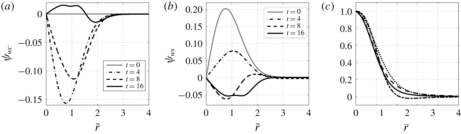
Figure 2(a,b) shows the streamfunctions  $\unicode[STIX]{x1D713}_{wc}$ and
 $\unicode[STIX]{x1D713}_{ws}$ plotted against
 $\tilde{r}$ at different times, for
 $F_{h}=0.1$ at
 $z=l_{z}/4$. In the next section, we will show that the angular velocity
 $\unicode[STIX]{x1D6FA}$ does not evolve with
 $\unicode[STIX]{x1D70F}$ in this plane. Hence, (3.44) and (3.45) have been integrated by imposing the initial angular velocity profile given by (2.11) for all time. We see that, after an initial transient phase, the streamfunctions globally decay with time in the vortex core.
Streamfunctions (a)  $\unicode[STIX]{x1D713}_{wc}$ and (b)
 $\unicode[STIX]{x1D713}_{ws}$ plotted against
 $\tilde{r}$ at
 $t=0$ (grey solid line),
 $t=4$ (black dash-dotted line),
 $t=8$ (black dashed line) and
 $t=16$ (black solid line), at
 $z=l_{z}/4$, where
 $\unicode[STIX]{x1D6FA}=[1-\exp (-\tilde{r}^{2})]/\tilde{r}^{2}$ regardless of
 $\unicode[STIX]{x1D70F}$. The Froude number is
 $F_{h}=0.1$. (c) Streamfunctions
 $\bar{\unicode[STIX]{x1D713}}_{2b}/(\unicode[STIX]{x1D6FD}_{2}\bar{r}^{2})$ (solid line),
 $\bar{\unicode[STIX]{x1D713}}_{2s}/(\unicode[STIX]{x1D70E}_{2}\bar{r}^{2})$ (dashed line),
 $\bar{\unicode[STIX]{x1D713}}_{2c}/(\unicode[STIX]{x1D712}_{2}\bar{r}^{2})$ (dash-dotted line) and
 $\bar{\unicode[STIX]{x1D713}}_{2s}^{\unicode[STIX]{x1D708}}/(\unicode[STIX]{x1D70E}_{2}^{\unicode[STIX]{x1D708}}\bar{r}^{2})$ (dotted line) computed in appendix D.

We have now fully determined the streamfunction at first order  $\unicode[STIX]{x1D713}_{11}$. It satisfies the boundary condition at
 $\tilde{r}=0$. However, it can be shown that it behaves for large
 $\tilde{r}$ as
 $$\begin{eqnarray}\displaystyle \unicode[STIX]{x1D713}_{11} & {\sim} & \displaystyle \left[\cos (\tilde{\unicode[STIX]{x1D703}})\frac{\unicode[STIX]{x2202}\unicode[STIX]{x1D6FF}y}{\unicode[STIX]{x2202}\unicode[STIX]{x1D70F}}-\sin (\tilde{\unicode[STIX]{x1D703}})\frac{\unicode[STIX]{x2202}\unicode[STIX]{x1D6FF}x}{\unicode[STIX]{x2202}\unicode[STIX]{x1D70F}}\right]\tilde{r}\nonumber\\ \displaystyle & & \displaystyle +\,\frac{{\mathcal{A}}}{2}\left[\cos (\tilde{\unicode[STIX]{x1D703}})\frac{\unicode[STIX]{x2202}^{2}\unicode[STIX]{x1D6FF}x}{\unicode[STIX]{x2202}\tilde{z}^{2}}+\sin (\tilde{\unicode[STIX]{x1D703}})\frac{\unicode[STIX]{x2202}^{2}\unicode[STIX]{x1D6FF}y}{\unicode[STIX]{x2202}\tilde{z}^{2}}\right]\tilde{r}+\cos (\tilde{\unicode[STIX]{x1D703}})\frac{{\mathcal{B}}t}{2}\frac{\text{d}U}{\text{d}\tilde{z}}\tilde{r}\nonumber\\ \displaystyle & & \displaystyle +\,\left[-\sin (\tilde{\unicode[STIX]{x1D703}})\unicode[STIX]{x1D717}+\cos (\tilde{\unicode[STIX]{x1D703}})\frac{{\mathcal{A}}t}{2}+\cos (\tilde{\unicode[STIX]{x1D703}})\frac{\unicode[STIX]{x2202}{\mathcal{S}}_{w}}{\unicode[STIX]{x2202}t}-\sin (\tilde{\unicode[STIX]{x1D703}})\frac{\unicode[STIX]{x2202}{\mathcal{C}}_{w}}{\unicode[STIX]{x2202}t}\right]\frac{\text{d}^{2}U}{\text{d}\tilde{z}^{2}}\tilde{r},\end{eqnarray}$$
where  ${\mathcal{A}}$ and
 ${\mathcal{B}}$ are given by
 $$\begin{eqnarray}\displaystyle & \displaystyle {\mathcal{A}}(\tilde{z},\unicode[STIX]{x1D70F})=\int _{0}^{+\infty }\unicode[STIX]{x1D709}^{2}\unicode[STIX]{x1D6FA}^{2}{\mathcal{C}}\,\text{d}\unicode[STIX]{x1D709}, & \displaystyle\end{eqnarray}$$
 $$\begin{eqnarray}\displaystyle & \displaystyle {\mathcal{B}}(\tilde{z},\unicode[STIX]{x1D70F})=\int _{0}^{+\infty }\unicode[STIX]{x1D709}^{2}\unicode[STIX]{x1D6FA}{\mathcal{C}}\left(3+{\mathcal{F}}\right)\frac{\unicode[STIX]{x2202}\unicode[STIX]{x1D6FA}}{\unicode[STIX]{x2202}\tilde{z}}\,\text{d}\unicode[STIX]{x1D709}\equiv \frac{\unicode[STIX]{x2202}{\mathcal{A}}}{\unicode[STIX]{x2202}\tilde{z}}, & \displaystyle\end{eqnarray}$$
where  ${\mathcal{C}}$ and
 ${\mathcal{F}}$ are defined in (3.25). Note that we have used the fact that
 $\unicode[STIX]{x1D713}_{wc}$ and
 $\unicode[STIX]{x1D713}_{ws}$ tend to zero as
 $\tilde{r}\rightarrow +\infty$.
In order to enforce the boundary condition  $\unicode[STIX]{x1D713}_{11}\rightarrow 0$ as
 $\tilde{r}\rightarrow +\infty$, we need to impose
 $$\begin{eqnarray}\displaystyle & \displaystyle \frac{\unicode[STIX]{x2202}\unicode[STIX]{x1D6FF}x}{\unicode[STIX]{x2202}\unicode[STIX]{x1D70F}}=\left[\frac{{\mathcal{A}}(\tilde{z},\unicode[STIX]{x1D70F})}{2}\frac{\unicode[STIX]{x2202}^{2}\unicode[STIX]{x1D6FF}y}{\unicode[STIX]{x2202}\tilde{z}^{2}}-\left(\unicode[STIX]{x1D717}(\tilde{z},\unicode[STIX]{x1D70F})+\frac{\unicode[STIX]{x2202}{\mathcal{C}}_{w}}{\unicode[STIX]{x2202}t}(t,\tilde{z},\unicode[STIX]{x1D70F})\right)\frac{\text{d}^{2}U}{\text{d}\tilde{z}^{2}}\right], & \displaystyle\end{eqnarray}$$
 $$\begin{eqnarray}\displaystyle & \displaystyle \frac{\unicode[STIX]{x2202}\unicode[STIX]{x1D6FF}y}{\unicode[STIX]{x2202}\unicode[STIX]{x1D70F}}=-\left[\frac{\unicode[STIX]{x2202}}{\unicode[STIX]{x2202}\tilde{z}}\left(\frac{{\mathcal{A}}(\tilde{z},\unicode[STIX]{x1D70F})}{2}t\frac{\text{d}U}{\text{d}\tilde{z}}\right)+\frac{{\mathcal{A}}(\tilde{z},\unicode[STIX]{x1D70F})}{2}\frac{\unicode[STIX]{x2202}^{2}\unicode[STIX]{x1D6FF}x}{\unicode[STIX]{x2202}\tilde{z}^{2}}+\frac{\unicode[STIX]{x2202}{\mathcal{S}}_{w}}{\unicode[STIX]{x2202}t}(t,\tilde{z},\unicode[STIX]{x1D70F})\frac{\text{d}^{2}U}{\text{d}\tilde{z}^{2}}\right]. & \displaystyle\end{eqnarray}$$
When  $U=0$, these equations are identical to those found by Billant (Reference Billant2010) for the self-induction of an isolated vortex in stratified non-rotating fluids.
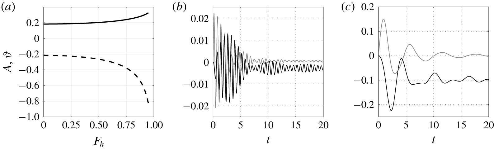
Figure 3(a) shows  ${\mathcal{A}}$ and
 $\unicode[STIX]{x1D717}$ as functions of
 $F_{h}$ at
 $z=l_{z}/4$, where the angular velocity remains the same,
 $\unicode[STIX]{x1D6FA}=[1-\exp (-\tilde{r}^{2})]/\tilde{r}^{2}$, independent of
 $\unicode[STIX]{x1D70F}$ (see § 4.1). They are almost independent of
 $F_{h}$ for
 $F_{h}\lesssim 0.5$. The wave forcing terms
 ${\mathcal{C}}_{w}$ and
 ${\mathcal{S}}_{w}$ are also shown in figure 3(b,c) for two Froude numbers
 $F_{h}=0.1$ and
 $F_{h}=0.5$, at the same location. In appendix E, it is shown that they behave for small time as
 $$\begin{eqnarray}{\mathcal{C}}_{w}=-\unicode[STIX]{x1D717}t+O(t^{3}),\quad {\mathcal{S}}_{w}=-\frac{{\mathcal{A}}}{4}t^{2}+O(t^{4}).\end{eqnarray}$$
Therefore, they initially compensate the effect of the shear flow in (3.52) and (3.53). Then, they go through oscillations as seen in figure 3(b,c). These oscillations exhibit two typical periods: the non-dimensional period of rotation in the vortex core,  $T\sim 2\unicode[STIX]{x03C0}$, and the buoyancy period,
 $T\sim 2\unicode[STIX]{x03C0}F_{h}$. For
 $F_{h}=0.5$ (figure 3c), these two periods are comparable so that
 ${\mathcal{C}}_{w}$ and
 ${\mathcal{S}}_{w}$ exhibit irregular oscillations, while for
 $F_{h}=0.1$ (figure 3b), fast oscillations superimposed on slow oscillations can be clearly distinguished. For large times,
 ${\mathcal{C}}_{w}$ and
 ${\mathcal{S}}_{w}$ tend to constant values because the waves are increasingly sheared by the vortex rotation through the terms
 $\cos (\unicode[STIX]{x1D6FA}t-\tilde{\unicode[STIX]{x1D703}})$ and
 $\sin (\unicode[STIX]{x1D6FA}t-\tilde{\unicode[STIX]{x1D703}})$ as seen in (3.23). As a result, their contributions
 $\unicode[STIX]{x2202}{\mathcal{C}}_{w}/\unicode[STIX]{x2202}t$ and
 $\unicode[STIX]{x2202}{\mathcal{S}}_{w}/\unicode[STIX]{x2202}t$ to the vortex displacements vanish as
 $t\rightarrow +\infty$.
(a) Variables  ${\mathcal{A}}$ (solid line) and
 $\unicode[STIX]{x1D717}$ (dashed line) plotted against
 $F_{h}$, at the vertical level
 $z=l_{z}/4$, where
 $\unicode[STIX]{x1D6FA}=[1-\exp (-\tilde{r}^{2})]/\tilde{r}^{2}$ regardless of
 $\unicode[STIX]{x1D70F}$. (b,c) Forcings
 ${\mathcal{C}}_{w}$ (grey lines) and
 ${\mathcal{S}}_{w}$ (black lines) for (b)
 $F_{h}=0.1$ and (c)
 $F_{h}=0.5$, at
 $z=l_{z}/4$.

In the next two sections, we will determine how the angular velocity evolves on the slow time  $\unicode[STIX]{x1D70F}$. Then, (3.52) and (3.53) will be solved in §4.2.
3.2.2 Determination of $(\unicode[STIX]{x1D6F7}_{10},\unicode[STIX]{x1D713}_{10})$

We now determine  $(\unicode[STIX]{x1D6F7}_{10},\unicode[STIX]{x1D713}_{10})$ corresponding to the azimuthal mode
 $m=0$ of the potential and streamfunction at first order (3.32). In order to keep the calculations relatively simple, we will assume here that the Froude number is small so that the hydrostatic approximation is satisfied. The comparison with the DNS in Part 2 will show that this assumption provides accurate predictions at least for
 $F_{h}\leqslant 0.5$. We will therefore take the limit
 $F_{h}\rightarrow 0$ of the vertical velocity and buoyancy (3.23) and (3.24). In addition, equations (3.52) and (3.53) for the displacement perturbations derived in the previous section show that
 $(\unicode[STIX]{x1D6FF}x,\unicode[STIX]{x1D6FF}y)$ remain of order unity for large time
 $t=O(1/\unicode[STIX]{x1D700})$ and are therefore small compared to the terms growing like
 $t$. Therefore, these displacements will be neglected in (3.23) and (3.24) in order to avoid lengthy calculations. Hence, (3.23) and (3.24) are simplified as follows:
 $$\begin{eqnarray}\displaystyle & \displaystyle w_{0}=\left[\cos (\tilde{\unicode[STIX]{x1D703}})-t\sin (\tilde{\unicode[STIX]{x1D703}})\unicode[STIX]{x1D6FA}-\cos (\unicode[STIX]{x1D6FA}t-\tilde{\unicode[STIX]{x1D703}})\cos \left(\frac{t}{F_{h}}\right)\right]\tilde{r}\unicode[STIX]{x1D6FA}^{2}\frac{\text{d}U}{\text{d}\tilde{z}}, & \displaystyle\end{eqnarray}$$
 $$\begin{eqnarray}\displaystyle & \displaystyle b_{0}=-t\cos (\tilde{\unicode[STIX]{x1D703}})\tilde{r}\unicode[STIX]{x1D6FA}^{2}\frac{\text{d}U}{\text{d}\tilde{z}}. & \displaystyle\end{eqnarray}$$
The only remaining term due to internal waves is the third term in (3.55). The forcing terms in (3.33) and (3.34) for  $m=0$ and
 $m=2$, i.e.
 $(\unicode[STIX]{x1D6FF}D_{0},\unicode[STIX]{x1D6FF}D_{2},\unicode[STIX]{x1D6FF}Z_{0},\unicode[STIX]{x1D6FF}Z_{2})$, have been derived using (3.55).
Equation (3.33) for the potential  $\unicode[STIX]{x1D6F7}_{10}$ reads
 $$\begin{eqnarray}\displaystyle \unicode[STIX]{x1D6FB}_{h}^{2}\unicode[STIX]{x1D6F7}_{10}=\left[\frac{\unicode[STIX]{x2202}\tilde{r}\unicode[STIX]{x1D6FA}}{\unicode[STIX]{x2202}\tilde{r}}-\left(\frac{\unicode[STIX]{x2202}\tilde{r}\unicode[STIX]{x1D6FA}}{\unicode[STIX]{x2202}\tilde{r}}\cos (\unicode[STIX]{x1D6FA}t)-\frac{t}{2}\tilde{r}\unicode[STIX]{x1D6FA}\frac{\unicode[STIX]{x2202}\unicode[STIX]{x1D6FA}}{\unicode[STIX]{x2202}\tilde{r}}\sin (\unicode[STIX]{x1D6FA}t)\right)\cos \left(\frac{t}{F_{h}}\right)\right]\unicode[STIX]{x1D6FA}t\left(\frac{\text{d}U}{\text{d}\tilde{z}}\right)^{2}. & & \displaystyle \nonumber\\ \displaystyle & & \displaystyle\end{eqnarray}$$
The solution, which is not singular at  $\tilde{r}=0$ and which vanishes at infinity, is
 $$\begin{eqnarray}\displaystyle \unicode[STIX]{x1D6F7}_{10}=\frac{t}{2}\left[\int _{+\infty }^{\tilde{r}}\unicode[STIX]{x1D709}\unicode[STIX]{x1D6FA}^{2}\,\text{d}\unicode[STIX]{x1D709}-\cos \left(\frac{t}{F_{h}}\right)\int _{+\infty }^{\tilde{r}}\unicode[STIX]{x1D709}\unicode[STIX]{x1D6FA}^{2}\cos (\unicode[STIX]{x1D6FA}t)\,\text{d}\unicode[STIX]{x1D709}\right]\left(\frac{\text{d}U}{\text{d}\tilde{z}}\right)^{2}. & & \displaystyle\end{eqnarray}$$
Using (3.58), equation (3.34) for the streamfunction  $\unicode[STIX]{x1D713}_{10}$ is
 $$\begin{eqnarray}\displaystyle \text{L}(\unicode[STIX]{x1D713}_{10})=-\frac{\unicode[STIX]{x2202}\unicode[STIX]{x1D701}_{0}}{\unicode[STIX]{x2202}\unicode[STIX]{x1D70F}}+{\mathcal{F}}_{10}, & & \displaystyle\end{eqnarray}$$
where
 $$\begin{eqnarray}\displaystyle & & \displaystyle {\mathcal{F}}_{10}=\left[-\frac{t}{\tilde{r}}\frac{\unicode[STIX]{x2202}\tilde{r}^{2}\unicode[STIX]{x1D6FA}^{3}}{\unicode[STIX]{x2202}\tilde{r}}-\left[\unicode[STIX]{x1D6FA}\left(\frac{\unicode[STIX]{x2202}\tilde{r}\unicode[STIX]{x1D6FA}}{\unicode[STIX]{x2202}\tilde{r}}+\frac{t^{2}}{2}\tilde{r}\unicode[STIX]{x1D6FA}^{2}\frac{\unicode[STIX]{x2202}\unicode[STIX]{x1D6FA}}{\unicode[STIX]{x2202}\tilde{r}}\right)\sin (\unicode[STIX]{x1D6FA}t)\right.\right.\nonumber\\ \displaystyle & & \displaystyle \quad \left.\left.-\;t\unicode[STIX]{x1D6FA}^{2}\frac{\unicode[STIX]{x2202}\tilde{r}\unicode[STIX]{x1D6FA}}{\unicode[STIX]{x2202}\tilde{r}}\cos (\unicode[STIX]{x1D6FA}t)\right]\cos \left(\frac{t}{F_{h}}\right)\right.+\left.\frac{\tilde{\unicode[STIX]{x1D70F}}^{2}}{2\tilde{Re}_{b}}\frac{1}{\tilde{r}}\frac{\unicode[STIX]{x2202}}{\unicode[STIX]{x2202}\tilde{r}}\left(\tilde{r}\frac{\unicode[STIX]{x2202}\unicode[STIX]{x1D701}_{0}}{\unicode[STIX]{x2202}\tilde{r}}\right)\right]\left(\frac{\text{d}U}{\text{d}\tilde{z}}\right)^{2},\end{eqnarray}$$
where we remind the reader that  $\tilde{\unicode[STIX]{x1D70F}}=\unicode[STIX]{x1D700}t$. Since
 $\unicode[STIX]{x1D713}_{10}$ is axisymmetric, the operator
 $\text{L}$ in (3.59) reduces to
 $\unicode[STIX]{x2202}\unicode[STIX]{x1D6FB}_{h}^{2}\unicode[STIX]{x1D713}_{10}/\unicode[STIX]{x2202}t$. In addition, we should impose that
 $$\begin{eqnarray}\left\langle \unicode[STIX]{x1D6FB}_{h}^{2}\unicode[STIX]{x1D713}_{10},\unicode[STIX]{x1D701}_{0}\right\rangle =0,\end{eqnarray}$$
in order that the vertical vorticity at first order is orthogonal to the vertical vorticity at leading order. Taking the scalar product of (3.59) with  $\unicode[STIX]{x1D701}_{0}$ shows that
 $\unicode[STIX]{x2202}\langle \unicode[STIX]{x1D6FB}_{h}^{2}\unicode[STIX]{x1D713}_{10},\unicode[STIX]{x1D701}_{0}\rangle /\unicode[STIX]{x2202}t=0$ only if
 $$\begin{eqnarray}\displaystyle \frac{\unicode[STIX]{x2202}\unicode[STIX]{x1D701}_{0}}{\unicode[STIX]{x2202}\unicode[STIX]{x1D70F}}={\mathcal{F}}_{10}. & & \displaystyle\end{eqnarray}$$
This equation describes the evolution of the leading-order vertical vorticity of the vortex (and associated angular velocity) over the slow time. It is analysed in § 4.1. The potential and streamfunction  $(\unicode[STIX]{x1D6F7}_{12},\unicode[STIX]{x1D713}_{12})$ are solved in appendix D.
4 Results
4.1 Evolution of the angular velocity of the vortex
Here, we analyse in detail the evolution equation (3.62) of the leading-order vertical vorticity. By rescaling the slow time, the vertical coordinate and the buoyancy Reynolds number, and by integrating in  $\tilde{r}$, we can derive from (3.62) an equation for the angular velocity
 $\unicode[STIX]{x1D6FA}$:
 $$\begin{eqnarray}\frac{\unicode[STIX]{x2202}\unicode[STIX]{x1D6FA}}{\unicode[STIX]{x2202}t}=\left[-F_{h}^{2}t\unicode[STIX]{x1D6FA}^{3}+\frac{F_{h}^{2}\unicode[STIX]{x1D6FA}^{2}}{2}\left(\unicode[STIX]{x1D6FA}t\cos (\unicode[STIX]{x1D6FA}t)-\sin (\unicode[STIX]{x1D6FA}t)\right)\cos \left(\frac{t}{F_{h}}\right)+\frac{t^{2}}{2Re\tilde{r}}\frac{\unicode[STIX]{x2202}\unicode[STIX]{x1D701}_{0}}{\unicode[STIX]{x2202}\tilde{r}}\right]\left(\frac{\text{d}U}{\text{d}z}\right)^{2}.\end{eqnarray}$$
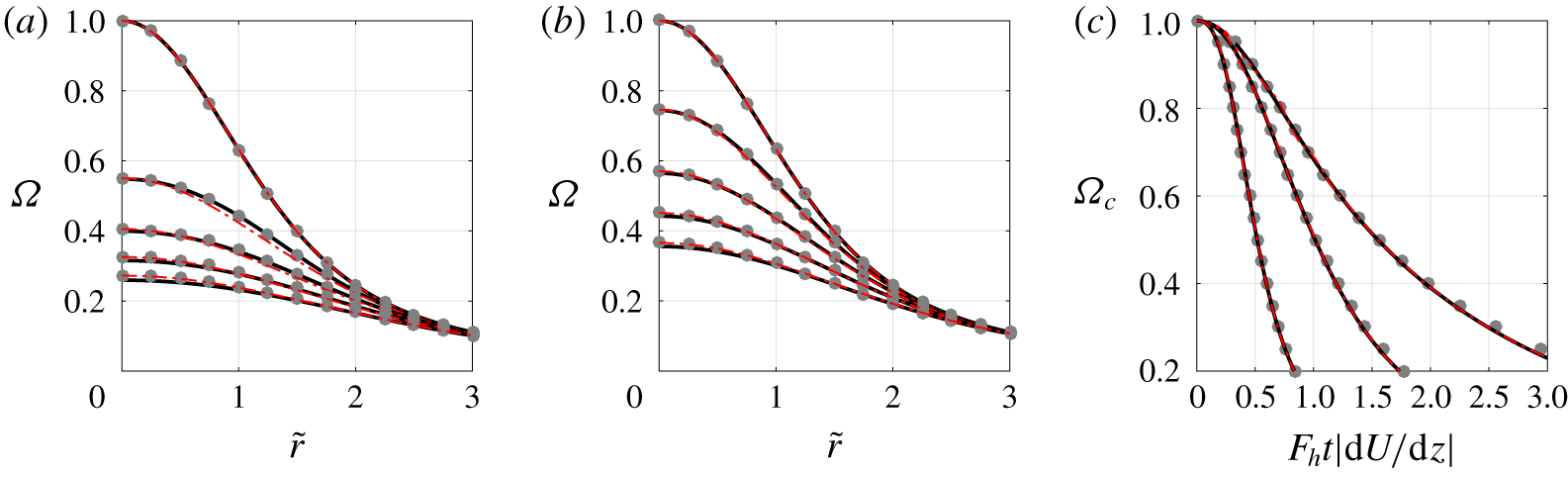
This equation shows that the angular velocity of the vortex decays because of dynamic and viscous effects (first and third terms on the right-hand side, respectively). The second term on the right-hand side corresponds to the effect of internal waves. However, we have observed that this effect is always weak. To illustrate this point, figure 5(c) (later in this section) shows that the angular velocity at the centre computed from (4.1) (black solid lines) is very close to the one computed by neglecting them (red lines), i.e. from
 $$\begin{eqnarray}\frac{\unicode[STIX]{x2202}\unicode[STIX]{x1D6FA}}{\unicode[STIX]{x2202}t}=\left[-F_{h}^{2}t\unicode[STIX]{x1D6FA}^{3}+\frac{t^{2}}{2Re\tilde{r}}\frac{\unicode[STIX]{x2202}\unicode[STIX]{x1D701}_{0}}{\unicode[STIX]{x2202}\tilde{r}}\right]\left(\frac{\text{d}U}{\text{d}z}\right)^{2}.\end{eqnarray}$$
We will therefore use this simplified equation in the following.
By equating the magnitude of the different terms in (4.2), it can be noticed that the intrinsic time scale of the equation is  $\tilde{\unicode[STIX]{x1D70F}}=\unicode[STIX]{x1D700}t$ if the buoyancy Reynolds number scales as
 $ReF_{h}^{2}=O(1/\unicode[STIX]{x1D700})$. However, it is not possible to perform a rigorous asymptotic analysis based on this time scale, as discussed in appendix A.
A physical interpretation of the origin of the dynamic effect (first term on the right-hand side of (4.2)) can be gained by considering the conservation of potential vorticity near the vortex axis when the vortex becomes tilted. First, let us consider the buoyancy at leading order  $b=\unicode[STIX]{x1D700}b_{0}/F_{h}=-t\tilde{x}\unicode[STIX]{x1D6FA}^{2}\,\text{d}U/\text{d}z$, where
 $b_{0}$ is given by (3.56) and
 $\tilde{x}=x-U(z)t$ (we neglect
 $\unicode[STIX]{x1D6FF}x$). Figure 4 sketches the lines of constant total buoyancy
 $b_{t}=b+z/F_{h}^{2}$ near the point
 $x=0$,
 $z=l_{z}/2$ at two times:
 $t=0$ (grey dashed lines) and
 $t=t_{0}$ (grey solid lines) where
 $t_{0}$ is small. At
 $t=t_{0}$, the vortex axis
 $\tilde{x}=0$ (bold solid line) is inclined towards the left since
 $x=U(z)t_{0}\simeq -k_{z}U_{S}t_{0}(z-l_{z}/2)$ near
 $z=l_{z}/2$. The iso-buoyancy lines are also no longer horizontal but slanted downwards towards the positive
 $x$ direction. On the vortex axis
 $\tilde{x}=0$, they remain at the same vertical level, while on the line
 $x=0$, they are displaced by
 $$\begin{eqnarray}\unicode[STIX]{x1D6FF}h=-F_{h}^{2}\unicode[STIX]{x1D6FA}^{2}ht_{0}^{2}\left(\frac{\text{d}U}{\text{d}z}\right)^{2},\end{eqnarray}$$
where  $h=z_{0}-l_{z}/2$ with
 $z_{0}$ the initial vertical level of the iso-buoyancy line. Therefore
 $\unicode[STIX]{x1D6FF}h$ is negative, as clearly seen in figure 4. Since the vortex is inclined, the iso-buoyancy lines are indeed displaced towards the vortex axis where the pressure is minimum. This means that the vortex is squeezed near
 $x=0$,
 $z=l_{z}/2$. The conservation of potential vorticity between the iso-density lines at
 $z=z_{0}$ and
 $z=l_{z}/2$ (figure 4),
 $$\begin{eqnarray}\frac{\unicode[STIX]{x1D701}}{h}=\frac{\unicode[STIX]{x1D701}+\unicode[STIX]{x1D6FF}\unicode[STIX]{x1D701}}{h+\unicode[STIX]{x1D6FF}h},\end{eqnarray}$$
implies that the vertical vorticity at  $t=t_{0}$ will decrease by
 $\unicode[STIX]{x1D6FF}\unicode[STIX]{x1D701}=\unicode[STIX]{x1D701}\unicode[STIX]{x1D6FF}h/h$. The variation of vertical vorticity between
 $t=0$ and
 $t=t_{0}$ is therefore
 $$\begin{eqnarray}\frac{\unicode[STIX]{x2202}\unicode[STIX]{x1D701}}{\unicode[STIX]{x2202}t}=\frac{\unicode[STIX]{x1D6FF}\unicode[STIX]{x1D701}}{t_{0}}=-F_{h}^{2}\unicode[STIX]{x1D701}\unicode[STIX]{x1D6FA}^{2}t_{0}\left(\frac{\text{d}U}{\text{d}z}\right)^{2}.\end{eqnarray}$$
This corresponds exactly to (4.2) for  $Re=\infty$ since
 $\unicode[STIX]{x1D701}=2\unicode[STIX]{x1D6FA}$ on the vortex axis. However, we stress that (4.2) is valid not only on the vortex axis near
 $z=l_{z}/2$ but everywhere.
Lines of constant total buoyancy  $b_{t}$ near the point
 $x=0$,
 $z=l_{z}/2$ at
 $t=0$ (grey dashed lines) and
 $t=t_{0}$ (grey solid lines). The bold black solid line represents the vortex axis at
 $t=t_{0}$. Here
 $\unicode[STIX]{x1D6FF}h$ is the height variation at
 $x=0$ of the iso-buoyancy line located at
 $z=h+l_{z}/2$ initially.

Both the dynamic and viscous decay of  $\unicode[STIX]{x1D6FA}$ are proportional to
 $(\text{d}U/\text{d}z)^{2}$. Hence, the decay will be maximum at
 $z=0,l_{z}/2$ and will vanish at
 $z=l_{z}/4$ and
 $3l_{z}/4$ for the sinusoidal profile
 $U=U_{S}\sin (k_{z}z)$. This explains why we have taken the initial angular velocity profile for computing the quantities at
 $z=l_{z}/4$ shown in figures 2 and 3.
Equation (4.2) can be solved by a multiple scale analysis. To do so, we introduce the time  $\tilde{t}=(F_{h}t|\text{d}U/\text{d}z|)^{3}$. Then, (4.2) becomes
 $$\begin{eqnarray}\frac{\unicode[STIX]{x2202}\unicode[STIX]{x1D6FA}}{\unicode[STIX]{x2202}\tilde{t}}=-\frac{\unicode[STIX]{x1D6FA}^{3}}{3\tilde{t}^{1/3}}+\frac{\unicode[STIX]{x1D6FE}}{6\tilde{r}}\frac{\unicode[STIX]{x2202}\unicode[STIX]{x1D701}_{0}}{\unicode[STIX]{x2202}\tilde{r}},\quad \text{where }\unicode[STIX]{x1D6FE}=1\bigg/\left(ReF_{h}^{3}\left|{\displaystyle \frac{\text{d}U}{\text{d}z}}\right|\right)\end{eqnarray}$$
is the only remaining control parameter. For a given set of parameters  $(F_{h},Re,k_{z},U_{S})$,
 $\unicode[STIX]{x1D6FE}$ lies between
 $1/(ReF_{h}^{3}k_{z}U_{S})$ and infinity as the vertical coordinate varies. For small
 $\unicode[STIX]{x1D6FE}$, the solution can be found as (appendix F.1)
 $$\begin{eqnarray}\unicode[STIX]{x1D6FA}=\frac{\unicode[STIX]{x1D6FA}_{i}}{\sqrt{1+\tilde{t}^{2/3}\unicode[STIX]{x1D6FA}_{i}^{2}}}-\frac{\unicode[STIX]{x1D6FE}}{2}\left({\displaystyle \frac{\unicode[STIX]{x2202}\unicode[STIX]{x1D6FA}_{i}}{\unicode[STIX]{x2202}\tilde{r}}}\right)^{2}\frac{3\arctan (\unicode[STIX]{x1D6FA}_{i}\tilde{t}^{1/3})-3\tilde{t}^{1/3}\unicode[STIX]{x1D6FA}_{i}+\tilde{t}\unicode[STIX]{x1D6FA}_{i}^{3}}{\unicode[STIX]{x1D6FA}_{i}^{4}\left(1+\tilde{t}^{2/3}\unicode[STIX]{x1D6FA}_{i}^{2}\right)^{3/2}}+O(\unicode[STIX]{x1D6FE}^{2}),\end{eqnarray}$$
with
 $$\begin{eqnarray}\unicode[STIX]{x1D6FA}_{i}=\frac{1}{\tilde{r}^{2}}\left[1-\exp \left(-{\displaystyle \frac{\tilde{r}^{2}}{1+2\unicode[STIX]{x1D6FE}\tilde{t}/3}}\right)\right].\end{eqnarray}$$
This approximation is only valid in the time range  $\tilde{t}\ll 1/\unicode[STIX]{x1D6FE}^{3}$. However, there is no particular interest in studying the solution for
 $\tilde{t}>1/\unicode[STIX]{x1D6FE}^{3}$ when
 $\unicode[STIX]{x1D6FE}\ll 1$ because, as shown in § 4.3, the shear is maximum when
 $\tilde{t}=O(1/\unicode[STIX]{x1D6FE})$, i.e. in the first time range
 $\tilde{t}\ll 1/\unicode[STIX]{x1D6FE}^{3}$. Equation (4.7) implies that the angular velocity at the vortex centre evolves as
 $$\begin{eqnarray}\unicode[STIX]{x1D6FA}_{c}=1/\sqrt{(1+2\unicode[STIX]{x1D6FE}\tilde{t}/3)^{2}+\tilde{t}^{2/3}}+O(\unicode[STIX]{x1D6FE}^{2}),\end{eqnarray}$$
i.e. in terms of  $t$ and the original parameters,
 $$\begin{eqnarray}\unicode[STIX]{x1D6FA}_{c}=1\left/\sqrt{\left[1+{\displaystyle \frac{2t^{3}}{3Re}}\left({\displaystyle \frac{\text{d}U}{\text{d}z}}\right)^{2}\right]^{2}+F_{h}^{2}t^{2}\left({\displaystyle \frac{\text{d}U}{\text{d}z}}\right)^{2}}.\right.\end{eqnarray}$$
In § F.2, we derive an approximation of the solution of (4.6) in the opposite limit:  $\unicode[STIX]{x1D6FE}\gg 1$. In this case, the angular velocity at leading order is given by
 $\unicode[STIX]{x1D6FA}=\unicode[STIX]{x1D6FA}_{i}$, where
 $\unicode[STIX]{x1D6FA}_{i}$ is defined in (4.8). However, the expressions (4.9) and (4.10) of
 $\unicode[STIX]{x1D6FA}_{c}$ derived for
 $\unicode[STIX]{x1D6FE}\ll 1$ turn out to be valid at leading order also when
 $\unicode[STIX]{x1D6FE}\gg 1$. Therefore, (4.10) will be used in the following and in Part 2 to describe the evolution of
 $\unicode[STIX]{x1D6FA}_{c}$ regardless of the value of
 $\unicode[STIX]{x1D6FE}$.
(a,b) Angular velocity profile  $\unicode[STIX]{x1D6FA}$ as a function of
 $\tilde{r}$ computed numerically from (4.6) (black solid lines) and predicted by (4.7) (grey circles) at different times for (a)
 $\unicode[STIX]{x1D6FE}=0.1$ and (b)
 $\unicode[STIX]{x1D6FE}=1$. The Lamb–Oseen profile (4.11) is also represented by red dash-dotted lines. The times shown are (a)
 $\tilde{t}=0$,
 $\tilde{t}=2.65$,
 $\tilde{t}=7.50$,
 $\tilde{t}=13.8$,
 $\tilde{t}=21.2$ and (b)
 $\tilde{t}=0$,
 $\tilde{t}=0.265$,
 $\tilde{t}=0.750$,
 $\tilde{t}=1.38$,
 $\tilde{t}=2.12$, from top to bottom. (c) Evolution of the angular velocity at the vortex centre
 $\unicode[STIX]{x1D6FA}_{c}$ as a function of
 $\tilde{t}^{1/3}=F_{h}t|\text{d}U/\text{d}z|$ predicted by (4.10) (grey circles) and computed numerically from (4.6) (black solid lines) for
 $\unicode[STIX]{x1D6FE}=0.1$,
 $\unicode[STIX]{x1D6FE}=1$ and
 $\unicode[STIX]{x1D6FE}=10$ (top to bottom). The red dash-dotted lines represent the numerical integration of the full equation (4.1) for
 $F_{h}=0.5$,
 $k_{z}=1$ and
 $U_{S}=0.2$.

Figure 5(a,b) compares the asymptotic solution (4.7) to the numerical solution of (4.6) at different times  $\tilde{t}$. We see that the agreement is excellent for
 $\unicode[STIX]{x1D6FE}=0.1$ (figure 5a) and even for
 $\unicode[STIX]{x1D6FE}=1$ (figure 5b). There are only some slight discrepancies in the vortex core
 $\tilde{r}\lesssim 1$ when
 $\tilde{t}\gtrsim 1$. In figure 5, the Lamb–Oseen profile
 $$\begin{eqnarray}\unicode[STIX]{x1D6FA}_{e}=\frac{1-\exp (-\tilde{r}^{2}/\tilde{a}_{e}^{2})}{\tilde{r}^{2}},\end{eqnarray}$$
with  $\tilde{a}_{e}^{2}=1/\unicode[STIX]{x1D6FA}_{c}$, where
 $\unicode[STIX]{x1D6FA}_{c}$ is given by (4.10), has also been plotted with black dash-dotted lines. This profile is close to the asymptotic solution (4.7). This is the reason why the empirical profile (4.11) is used in appendix D to ease the numerical resolution of the streamfunction
 $\unicode[STIX]{x1D713}_{12}$.
Figure 5(c) shows the asymptotic angular velocity at the vortex centre (4.10) and the numerical solution of (4.6) for different values of the control parameter  $\unicode[STIX]{x1D6FE}$. The agreement is very good not only for
 $\unicode[STIX]{x1D6FE}=0.1$ but also for
 $\unicode[STIX]{x1D6FE}=1$ and for
 $\unicode[STIX]{x1D6FE}=10$, confirming that (4.10) is a valid approximation of
 $\unicode[STIX]{x1D6FA}_{c}$ whatever the magnitude of
 $\unicode[STIX]{x1D6FE}$.
4.2 Analysis of the vortex deformations
Having determined the evolution of  $\unicode[STIX]{x1D6FA}$, we now come back to the study of equations (3.52) and (3.53) for the vortex displacements.
4.2.1 General solution
To solve (3.52) and (3.53), it is first convenient to rescale the slow time  $\unicode[STIX]{x1D70F}$ in terms of the time
 $t$:
 $$\begin{eqnarray}\displaystyle & \displaystyle \frac{\unicode[STIX]{x2202}\unicode[STIX]{x1D6FF}x}{\unicode[STIX]{x2202}t}=\left[\frac{{\mathcal{A}}(\tilde{z},t)}{2}\frac{\unicode[STIX]{x2202}^{2}\unicode[STIX]{x1D6FF}y}{\unicode[STIX]{x2202}\tilde{z}^{2}}-\left(\unicode[STIX]{x1D717}(\tilde{z},t)+\frac{\unicode[STIX]{x2202}{\mathcal{C}}_{w}}{\unicode[STIX]{x2202}t}(\tilde{z},t)\right)\frac{\text{d}^{2}U}{\text{d}\tilde{z}^{2}}\right]\unicode[STIX]{x1D700}^{2}, & \displaystyle\end{eqnarray}$$
 $$\begin{eqnarray}\displaystyle & \displaystyle \frac{\unicode[STIX]{x2202}\unicode[STIX]{x1D6FF}y}{\unicode[STIX]{x2202}t}=-\left[\frac{\unicode[STIX]{x2202}}{\unicode[STIX]{x2202}\tilde{z}}\left(\frac{{\mathcal{A}}(\tilde{z},t)}{2}t\frac{\text{d}U}{\text{d}\tilde{z}}\right)+\frac{{\mathcal{A}}(\tilde{z},t)}{2}\frac{\unicode[STIX]{x2202}^{2}\unicode[STIX]{x1D6FF}x}{\unicode[STIX]{x2202}\tilde{z}^{2}}+\frac{\unicode[STIX]{x2202}{\mathcal{S}}_{w}}{\unicode[STIX]{x2202}t}(\tilde{z},t)\frac{\text{d}^{2}U}{\text{d}\tilde{z}^{2}}\right]\unicode[STIX]{x1D700}^{2}. & \displaystyle\end{eqnarray}$$
The solution of (4.12) and (4.13) can be decomposed as
 $$\begin{eqnarray}\displaystyle & \displaystyle \unicode[STIX]{x1D6FF}x=\unicode[STIX]{x1D6FF}x^{\ast }-\unicode[STIX]{x1D700}^{2}\left[{\mathcal{C}}_{w}+\int _{0}^{t}\unicode[STIX]{x1D717}(\tilde{z},\unicode[STIX]{x1D710})\,\text{d}\unicode[STIX]{x1D710}\right]\frac{\text{d}^{2}U}{\text{d}\tilde{z}^{2}}, & \displaystyle\end{eqnarray}$$
 $$\begin{eqnarray}\displaystyle & \displaystyle \unicode[STIX]{x1D6FF}y=\unicode[STIX]{x1D6FF}y^{\ast }-\unicode[STIX]{x1D700}^{2}\left[{\mathcal{S}}_{w}\frac{\text{d}^{2}U}{\text{d}\tilde{z}^{2}}+\int _{0}^{t}\frac{\unicode[STIX]{x2202}}{\unicode[STIX]{x2202}\tilde{z}}\left(\frac{{\mathcal{A}}(\tilde{z},\unicode[STIX]{x1D710})}{2}\frac{\text{d}U}{\text{d}\tilde{z}}\right)\unicode[STIX]{x1D710}\,\text{d}\unicode[STIX]{x1D710}\right], & \displaystyle\end{eqnarray}$$
giving
 $$\begin{eqnarray}\displaystyle & \displaystyle \frac{\unicode[STIX]{x2202}\unicode[STIX]{x1D6FF}x^{\ast }}{\unicode[STIX]{x2202}t}=\hat{\unicode[STIX]{x1D714}}\frac{\unicode[STIX]{x2202}^{2}\unicode[STIX]{x1D6FF}y^{\ast }}{\unicode[STIX]{x2202}\tilde{z}^{2}}+O(\unicode[STIX]{x1D700}^{4}), & \displaystyle\end{eqnarray}$$
 $$\begin{eqnarray}\displaystyle & \displaystyle \frac{\unicode[STIX]{x2202}\unicode[STIX]{x1D6FF}y^{\ast }}{\unicode[STIX]{x2202}t}=-\hat{\unicode[STIX]{x1D714}}\frac{\unicode[STIX]{x2202}^{2}\unicode[STIX]{x1D6FF}x^{\ast }}{\unicode[STIX]{x2202}\tilde{z}^{2}}+O(\unicode[STIX]{x1D700}^{4}), & \displaystyle\end{eqnarray}$$
where  $\hat{\unicode[STIX]{x1D714}}=\unicode[STIX]{x1D700}^{2}{\mathcal{A}}/2$. Since (4.12) and (4.13) are valid up to order
 $O(\unicode[STIX]{x1D700}^{2})$, it is indeed legitimate to neglect the terms
 $O(\unicode[STIX]{x1D700}^{4})$ in (4.16) and (4.17). Since
 $\hat{\unicode[STIX]{x1D714}}$ is small, an approximation of the solution of (4.16) and (4.17) can be found in the form
 $$\begin{eqnarray}\displaystyle & \displaystyle \unicode[STIX]{x1D6FF}x^{\ast }=\text{e}^{\text{i}\tilde{k}_{z}\tilde{z}}\left[\unicode[STIX]{x1D6FF}x_{c}^{\ast }\cos \left(\int _{0}^{t}\hat{\unicode[STIX]{x1D714}}(z,\unicode[STIX]{x1D710})\,\text{d}\unicode[STIX]{x1D710}\right)+\unicode[STIX]{x1D6FF}x_{s}^{\ast }\sin \left(\int _{0}^{t}\hat{\unicode[STIX]{x1D714}}(z,\unicode[STIX]{x1D710})\,\text{d}\unicode[STIX]{x1D710}\right)\right]+\text{c.c.}, & \displaystyle\end{eqnarray}$$
 $$\begin{eqnarray}\displaystyle & \displaystyle \unicode[STIX]{x1D6FF}y^{\ast }=\text{e}^{\text{i}\tilde{k}_{z}\tilde{z}}\left[-\unicode[STIX]{x1D6FF}x_{s}^{\ast }\cos \left(\int _{0}^{t}\hat{\unicode[STIX]{x1D714}}(z,\unicode[STIX]{x1D710})\,\text{d}\unicode[STIX]{x1D710}\right)+\unicode[STIX]{x1D6FF}x_{c}^{\ast }\sin \left(\int _{0}^{t}\hat{\unicode[STIX]{x1D714}}(z,\unicode[STIX]{x1D710})\,\text{d}\unicode[STIX]{x1D710}\right)\right]+\text{c.c.},\quad & \displaystyle\end{eqnarray}$$
where  $\unicode[STIX]{x1D6FF}x_{c}^{\ast }$ and
 $\unicode[STIX]{x1D6FF}x_{s}^{\ast }$ are constants. The initial conditions
 $\unicode[STIX]{x1D6FF}x=\unicode[STIX]{x1D6FF}y=0$ at
 $t=0$ impose
 $\unicode[STIX]{x1D6FF}x_{c}^{\ast }=\unicode[STIX]{x1D6FF}x_{s}^{\ast }=0$. Therefore, a solution of (4.12) and (4.13) valid up to order
 $O(\unicode[STIX]{x1D700}^{2})$ is
 $$\begin{eqnarray}\displaystyle & \displaystyle \unicode[STIX]{x1D6FF}x=-\unicode[STIX]{x1D700}^{2}\left[{\mathcal{C}}_{w}+\int _{0}^{t}\unicode[STIX]{x1D717}(\tilde{z},\unicode[STIX]{x1D710})\,\text{d}\unicode[STIX]{x1D710}\right]\frac{\text{d}^{2}U}{\text{d}\tilde{z}^{2}}, & \displaystyle\end{eqnarray}$$
 $$\begin{eqnarray}\displaystyle & \displaystyle \unicode[STIX]{x1D6FF}y=-\unicode[STIX]{x1D700}^{2}\left[{\mathcal{S}}_{w}\frac{\text{d}^{2}U}{\text{d}\tilde{z}^{2}}+\int _{0}^{t}\frac{\unicode[STIX]{x2202}}{\unicode[STIX]{x2202}\tilde{z}}\left(\frac{{\mathcal{A}}(\tilde{z},\unicode[STIX]{x1D710})}{2}\frac{\text{d}U}{\text{d}\tilde{z}}\right)\unicode[STIX]{x1D710}\,\text{d}\unicode[STIX]{x1D710}\right]. & \displaystyle\end{eqnarray}$$
These equations show that the vortex axis evolves because of three different effects in addition to the advection  $Ut\boldsymbol{e}_{x}$ by the shear flow:
(i) the displacement due to internal waves (first terms on the right-hand side of (4.20) and (4.21));
(ii) the second term on the right-hand side of (4.20), which describes a small delay (since
$\unicode[STIX]{x1D717}$ is negative as seen in figure 3a) in the advection by the shear flow due to its vertical variations;(iii) the self-induction (second term on the right-hand side of (4.21)) – the shear flow bends the vortex in the
$x$ direction and, in turn, this creates a self-induced motion in the $y$ direction; this effect is modulated along the vertical since ${\mathcal{A}}$ varies via the vertical variation of the angular velocity of the vortex.


For large time such that  $\tilde{\unicode[STIX]{x1D70F}}=\unicode[STIX]{x1D700}t=O(1)$, (4.20) and (4.21) reduce at leading order to
 $$\begin{eqnarray}\displaystyle & \displaystyle \unicode[STIX]{x1D6FF}x=-\unicode[STIX]{x1D700}\int _{0}^{\tilde{\unicode[STIX]{x1D70F}}}\unicode[STIX]{x1D717}\,\text{d}\unicode[STIX]{x1D710}\,\frac{\text{d}^{2}U}{\text{d}\tilde{z}^{2}}, & \displaystyle\end{eqnarray}$$
 $$\begin{eqnarray}\displaystyle & \displaystyle \unicode[STIX]{x1D6FF}y=-\int _{0}^{\tilde{\unicode[STIX]{x1D70F}}}\frac{\unicode[STIX]{x2202}}{\unicode[STIX]{x2202}\tilde{z}}\left(\frac{{\mathcal{A}}}{2}\frac{\text{d}U}{\text{d}\tilde{z}}\right)\unicode[STIX]{x1D710}\,\text{d}\unicode[STIX]{x1D710}, & \displaystyle\end{eqnarray}$$
where we remind the reader that  $\unicode[STIX]{x1D717}$ and
 ${\mathcal{A}}$ are defined in (3.47) and (3.50). These expressions show that the displacements are
 $\unicode[STIX]{x1D6FF}y=O(1)$, while
 $\unicode[STIX]{x1D6FF}x=O(\unicode[STIX]{x1D700})$ for
 $t\sim 1/\unicode[STIX]{x1D700}$. The effect of internal waves remains
 $O(\unicode[STIX]{x1D700}^{2})$ and is thus negligible. This is the reason why we have neglected
 $(\unicode[STIX]{x1D6FF}x,\unicode[STIX]{x1D6FF}y)$ compared to
 $U(\tilde{z})t$ in § 3.2.2.
4.2.2 Behaviour for small time
By substituting  ${\mathcal{C}}_{w}$ and
 ${\mathcal{S}}_{w}$ in (4.20) and (4.21) by their asymptotic expressions (E 12) derived for small time (see appendix E) and by assuming that the angular velocity does not evolve for small time, we find that the displacements behave for
 $t\ll 1$ as
 $$\begin{eqnarray}\unicode[STIX]{x1D6FF}x=k_{z}^{2}\unicode[STIX]{x1D70D}t^{3}\frac{\text{d}^{2}U}{\text{d}\tilde{z}^{2}}+O(t^{4}),\quad \unicode[STIX]{x1D6FF}y=k_{z}^{2}\unicode[STIX]{x1D70E}t^{4}\frac{\text{d}^{2}U}{\text{d}\tilde{z}^{2}}+O(t^{5}),\end{eqnarray}$$
where  $\unicode[STIX]{x1D70D}$ and
 $\unicode[STIX]{x1D70E}$ are constants given in (E 13).
Remarkably, the initial evolution of  $(\unicode[STIX]{x1D6FF}x,\unicode[STIX]{x1D6FF}y)$ is independent of the Froude number at leading order. At this order,
 $\unicode[STIX]{x1D6FF}x$ and
 $\unicode[STIX]{x1D6FF}y$ vary like
 $t^{3}$ and
 $t^{4}$, respectively. It is interesting to compare the predictions (4.24) to those of a heuristic model where the advection by the shear flow is directly added to the equations of the self-induced motion of the single vortex, i.e.
 $$\begin{eqnarray}\displaystyle & \displaystyle \frac{\unicode[STIX]{x2202}\unicode[STIX]{x0394}x}{\unicode[STIX]{x2202}t}=\hat{\unicode[STIX]{x1D714}}\frac{\unicode[STIX]{x2202}^{2}\unicode[STIX]{x1D6FF}y}{\unicode[STIX]{x2202}\tilde{z}^{2}}+U(\tilde{z}), & \displaystyle\end{eqnarray}$$
 $$\begin{eqnarray}\displaystyle & \displaystyle \frac{\unicode[STIX]{x2202}\unicode[STIX]{x1D6FF}y}{\unicode[STIX]{x2202}t}=-\hat{\unicode[STIX]{x1D714}}\frac{\unicode[STIX]{x2202}^{2}\unicode[STIX]{x0394}x}{\unicode[STIX]{x2202}\tilde{z}^{2}}, & \displaystyle\end{eqnarray}$$
where  $\unicode[STIX]{x0394}x=U(\tilde{z})t+\unicode[STIX]{x1D6FF}x$ is the total displacement of the vortex in the streamwise direction. Such a phenomenological model can be obtained from (4.12) and (4.13) by setting
 $\unicode[STIX]{x2202}{\mathcal{C}}_{w}/\unicode[STIX]{x2202}t=\unicode[STIX]{x2202}{\mathcal{S}}_{w}/\unicode[STIX]{x2202}t=\unicode[STIX]{x1D717}=0$ and
 $\unicode[STIX]{x2202}\unicode[STIX]{x1D6FA}_{c}/\unicode[STIX]{x2202}\tilde{z}=0$, i.e. by neglecting the effect of the waves, the three-dimensional correction of the advection by the base flow and by assuming that the angular velocity remains constant with time. The model (4.25) and (4.26) has been introduced, for example, by Marshall & Parthasarathy (Reference Marshall and Parthasarathy1993) for two-layer quasi-geostrophic flows. For small times
 $t\ll 1$, the solution of (4.25) and (4.26) is
 $$\begin{eqnarray}\unicode[STIX]{x1D6FF}x=-\frac{\hat{\unicode[STIX]{x1D714}}^{2}}{6}t^{3}\frac{\text{d}^{4}U}{\text{d}\tilde{z}^{4}}+O(t^{4}),\quad \unicode[STIX]{x1D6FF}y=-\frac{\hat{\unicode[STIX]{x1D714}}}{2}t^{2}\frac{\text{d}^{2}U}{\text{d}\tilde{z}^{2}}+O(t^{3}).\end{eqnarray}$$
Thus,  $\unicode[STIX]{x1D6FF}x$ is initially of order
 $k_{z}^{4}F_{h}^{4}t^{3}$ instead of
 $k_{z}^{2}t^{3}$, and
 $\unicode[STIX]{x1D6FF}y$ is of order
 $k_{z}^{2}F_{h}^{2}t^{2}$ instead of
 $k_{z}^{2}t^{4}$. This shows that internal waves have an important effect on the initial dynamics of the vortex. (Note, however, that such waves should be absent in the quasi-geostrophic limit considered by Marshall & Parthasarathy (Reference Marshall and Parthasarathy1993).)
4.3 Evolution of the Richardson number
From the asymptotic expressions of the velocity and buoyancy fields, it is now possible to predict the evolution of the Richardson number:
 $$\begin{eqnarray}Ri={\displaystyle \frac{{\displaystyle \frac{1}{F_{h}^{2}}}+{\displaystyle \frac{\unicode[STIX]{x2202}b}{\unicode[STIX]{x2202}z}}}{\left({\displaystyle \frac{\unicode[STIX]{x2202}u}{\unicode[STIX]{x2202}z}}\right)^{2}+\left({\displaystyle \frac{\unicode[STIX]{x2202}v}{\unicode[STIX]{x2202}z}}\right)^{2}}}.\end{eqnarray}$$
In the DNS performed in Part 2, we will see that the Richardson number reaches its minimum or the Kelvin–Helmholtz instability first appears at the vortex centre  $\tilde{r}=0$ and at the levels
 $z=0$ and
 $l_{z}/2$ where the ambient shear is maximum. In the following, we will therefore focus on the point
 $(\tilde{r}=0,z=l_{z}/2)$ (the point
 $(\tilde{r}=0,z=0)$ is equivalent due to the symmetry of the ambient shear flow).
The vertical shear of the horizontal velocity at this location can be computed by using the expansion of the velocity field (3.4) and the expression of the total derivative (3.12) (or (3.19)). This leads to
 $$\begin{eqnarray}\displaystyle \frac{\unicode[STIX]{x2202}u_{c}}{\unicode[STIX]{x2202}z} & = & \displaystyle k_{z}U_{S}^{3}\unicode[STIX]{x1D700}^{2}t\left[\left(\frac{3}{4}-\unicode[STIX]{x1D70E}_{2}\right)t\unicode[STIX]{x1D6FA}_{c}^{2}-\frac{\unicode[STIX]{x1D70E}_{2}^{\unicode[STIX]{x1D708}}t^{2}\unicode[STIX]{x1D6FA}_{c}}{ReF_{h}^{2}}\right]+\unicode[STIX]{x1D6FA}_{c}\frac{\unicode[STIX]{x2202}\unicode[STIX]{x1D6FF}y_{c}}{\unicode[STIX]{x2202}z}\nonumber\\ \displaystyle & & \displaystyle -\,k_{z}U_{S}+k_{z}\unicode[STIX]{x1D700}^{2}U_{S}\left({\mathcal{D}}_{c}+\unicode[STIX]{x1D706}_{0c}\unicode[STIX]{x1D6FA}_{c}+\unicode[STIX]{x1D706}_{1c}-\unicode[STIX]{x1D717}_{c}\right),\end{eqnarray}$$
 $$\begin{eqnarray}\displaystyle \frac{\unicode[STIX]{x2202}v_{c}}{\unicode[STIX]{x2202}z} & = & \displaystyle k_{z}U_{S}t\unicode[STIX]{x1D6FA}_{c}-k_{z}U_{S}^{3}\unicode[STIX]{x1D700}^{2}t\left[\unicode[STIX]{x1D6FD}_{2}\unicode[STIX]{x1D6FA}_{c}+\left(\frac{1}{4}+\unicode[STIX]{x1D712}_{2}\right)t^{2}\unicode[STIX]{x1D6FA}_{c}^{3}\right]-\unicode[STIX]{x1D6FA}_{c}\frac{\unicode[STIX]{x2202}\unicode[STIX]{x1D6FF}x_{c}}{\unicode[STIX]{x2202}z}\nonumber\\ \displaystyle & & \displaystyle -\,k_{z}U_{S}t\left[\unicode[STIX]{x1D700}^{2}\left(\unicode[STIX]{x1D706}_{1c}\unicode[STIX]{x1D6FA}_{c}+{\mathcal{D}}_{c}\unicode[STIX]{x1D6FA}_{c}+\frac{{\mathcal{A}}_{c}}{2}\right)\right.\nonumber\\ \displaystyle & & \displaystyle \left.-\,\frac{F_{h}^{2}}{2}\frac{\unicode[STIX]{x2202}^{2}{\mathcal{A}}_{c}}{\unicode[STIX]{x2202}z^{2}}-F_{h}^{2}\unicode[STIX]{x1D6FA}_{c}\left(\frac{3}{2}\frac{\unicode[STIX]{x2202}^{2}{\mathcal{D}}_{c}}{\unicode[STIX]{x2202}z^{2}}-\frac{\unicode[STIX]{x2202}\unicode[STIX]{x1D706}_{c}}{\unicode[STIX]{x2202}z}\right)\right],\end{eqnarray}$$
where the subscript  $c$ indicates that the values are computed at
 $(\tilde{r}=0,z=l_{z}/2)$ or
 $z=l_{z}/2$ for the quantities independent of
 $\tilde{r}$. The terms in the first line on the right-hand sides of (4.29) and (4.30) come from the horizontal derivatives, while those in the next lines originate from the vertical derivative at constant horizontal coordinates (see (3.12)). The terms of order
 $\unicode[STIX]{x1D700}^{4}$ have been neglected. In particular, the fact that
 $(\unicode[STIX]{x1D6FF}x,\unicode[STIX]{x1D6FF}y)$ are formally of order
 $\unicode[STIX]{x1D700}^{2}$ (see (4.20) and (4.21)) has been used. The internal waves have been omitted in (4.29) and (4.30) for the reasons explained in § 3.1. The coefficients
 $\unicode[STIX]{x1D6FD}_{2}$,
 $\unicode[STIX]{x1D70E}_{2}$,
 $\unicode[STIX]{x1D712}_{2}$ and
 $\unicode[STIX]{x1D70E}_{2}^{\unicode[STIX]{x1D708}}$ are given in equations (D 15). The parameters
 $(\unicode[STIX]{x1D706}_{0},\unicode[STIX]{x1D706}_{1},\unicode[STIX]{x1D706})$,
 $\unicode[STIX]{x1D717}$ and
 ${\mathcal{A}}$ are defined in (3.42), (3.47) and (3.50), respectively. The parameter
 ${\mathcal{D}}$ is
 $$\begin{eqnarray}\displaystyle {\mathcal{D}}=\int _{0}^{+\infty }\unicode[STIX]{x1D709}\unicode[STIX]{x1D6FA}^{2}\,\text{d}\unicode[STIX]{x1D709}. & & \displaystyle\end{eqnarray}$$
Similarly, the total vertical derivative of the buoyancy at  $\tilde{r}=0,z=l_{z}/2$ can be obtained from the leading-order expression of the buoyancy in the hydrostatic limit (3.56):
 $$\begin{eqnarray}\frac{\unicode[STIX]{x2202}b_{c}}{\unicode[STIX]{x2202}z}=\left(k_{z}U_{S}t-\frac{\unicode[STIX]{x2202}\unicode[STIX]{x1D6FF}x_{c}}{\unicode[STIX]{x2202}z}\right)k_{z}U_{S}t\unicode[STIX]{x1D6FA}_{c}^{2}.\end{eqnarray}$$
Figure 6(a,b) shows one example of the evolution of  $\unicode[STIX]{x2202}u_{c}/\unicode[STIX]{x2202}z$,
 $\unicode[STIX]{x2202}v_{c}/\unicode[STIX]{x2202}z$ and
 $\unicode[STIX]{x2202}b_{c}/\unicode[STIX]{x2202}z$ predicted by (4.29), (4.30) and (4.32) (solid lines). They all reach a maximum value at a finite time. Remarkably, the magnitude of
 $\unicode[STIX]{x2202}u_{c}/\unicode[STIX]{x2202}z$ is much lower than
 $\unicode[STIX]{x2202}v_{c}/\unicode[STIX]{x2202}z$. As seen in figure 6(c), the corresponding Richardson number
 $Ri_{c}$ reaches a minimum value approximately equal to
 $4$. In the inviscid limit, represented by dash-dotted lines,
 $\unicode[STIX]{x2202}v_{c}/\unicode[STIX]{x2202}z$,
 $\unicode[STIX]{x2202}b_{c}/\unicode[STIX]{x2202}z$ and
 $Ri_{c}$ saturate to finite values as
 $t\rightarrow \infty$. The saturation of
 $\unicode[STIX]{x2202}v_{c}/\unicode[STIX]{x2202}z$ is intimately linked to the decay of the angular velocity of the vortex due to the squeezing of the isopycnal surfaces and potential vorticity conservation. The same effect is responsible for the growth and saturation of
 $\unicode[STIX]{x2202}b_{c}/\unicode[STIX]{x2202}z$.
Evolution of (a)  $\unicode[STIX]{x2202}u_{c}/\unicode[STIX]{x2202}z$ (grey lines) and
 $\unicode[STIX]{x2202}v_{c}/\unicode[STIX]{x2202}z$ (black lines), (b)
 $\unicode[STIX]{x2202}b/\unicode[STIX]{x2202}z$ and (c)
 $Ri_{c}$ predicted by (4.29), (4.30) and (4.32) for
 $F_{h}=0.1$,
 $k_{z}=2$,
 $U_{S}=0.2$ and for
 $Re=6000$ (solid lines) and
 $Re=\infty$ (dash-dotted lines). The dashed lines represent the predictions from the approximations (4.33), (4.34), (4.35) and (4.36).

To study the extrema of the quantities (4.29), (4.30) and (4.32), it is convenient to rewrite them as
 $$\begin{eqnarray}\displaystyle & \displaystyle \frac{\unicode[STIX]{x2202}u_{c}}{\unicode[STIX]{x2202}z}=\frac{\unicode[STIX]{x1D700}U_{S}}{F_{h}}\left[-1+\left(\frac{3}{4}-\unicode[STIX]{x1D70E}_{2}\right)\unicode[STIX]{x1D702}^{2}-\frac{\unicode[STIX]{x1D70E}_{2}^{\unicode[STIX]{x1D708}}\unicode[STIX]{x1D702}^{3}\unicode[STIX]{x1D6FE}_{c}}{\unicode[STIX]{x1D6FA}_{c}^{2}}+O(\unicode[STIX]{x1D700}^{2})\right], & \displaystyle\end{eqnarray}$$
 $$\begin{eqnarray}\displaystyle & \displaystyle \frac{\unicode[STIX]{x2202}v_{c}}{\unicode[STIX]{x2202}z}=\frac{\unicode[STIX]{x1D702}}{F_{h}}\left[1-\left(\frac{1}{4}+\unicode[STIX]{x1D712}_{2}\right)\unicode[STIX]{x1D702}^{2}+O(\unicode[STIX]{x1D700}^{2})\right], & \displaystyle\end{eqnarray}$$
 $$\begin{eqnarray}\displaystyle & \displaystyle \frac{\unicode[STIX]{x2202}b_{c}}{\unicode[STIX]{x2202}z}=\frac{\unicode[STIX]{x1D702}^{2}}{F_{h}^{2}}\left[1+O(\unicode[STIX]{x1D700}^{2})\right], & \displaystyle\end{eqnarray}$$
where  $\unicode[STIX]{x1D702}=\unicode[STIX]{x1D700}U_{S}t\unicode[STIX]{x1D6FA}_{c}$ and
 $\unicode[STIX]{x1D6FE}_{c}=\unicode[STIX]{x1D6FE}(z=l_{z}/2)=1/(ReF_{h}^{3}k_{z}U_{S})$. This shows that
 $\unicode[STIX]{x2202}v_{c}/\unicode[STIX]{x2202}z$ and
 $\unicode[STIX]{x2202}b_{c}/\unicode[STIX]{x2202}z$ depend on time only through
 $\unicode[STIX]{x1D702}$ at leading order in
 $\unicode[STIX]{x1D700}$. We see also that
 $\unicode[STIX]{x2202}u_{c}/\unicode[STIX]{x2202}z$ is one order in
 $\unicode[STIX]{x1D700}$ smaller than
 $\unicode[STIX]{x2202}v_{c}/\unicode[STIX]{x2202}z$ and
 $\unicode[STIX]{x2202}b_{c}/\unicode[STIX]{x2202}z$ for
 $\unicode[STIX]{x1D702}=O(1)$. We can notice that the last two terms of (4.34) are of order unity when
 $\unicode[STIX]{x1D702}=O(1)$. They are therefore of the same order as the leading-order term, although they originate from first-order terms in the asymptotic analysis (i.e.
 $O(\unicode[STIX]{x1D700}^{2})$). This clearly shows that the asymptotic analysis is non-uniform in time.
These approximations imply that, at leading order in  $\unicode[STIX]{x1D700}$,
 $Ri_{c}$ reads as
 $$\begin{eqnarray}Ri_{c}={\displaystyle \frac{1+\unicode[STIX]{x1D702}^{2}}{\unicode[STIX]{x1D702}^{2}[1-({\textstyle \frac{1}{4}}+\unicode[STIX]{x1D712}_{2})\unicode[STIX]{x1D702}^{2}]^{2}}}.\end{eqnarray}$$
As seen by the dashed lines in figure 6, the approximations (4.33)–(4.36) are very close to the full predictions by (4.29)–(4.32).
The approximations (4.34)–(4.36) show that the three quantities  $\unicode[STIX]{x2202}v_{c}/\unicode[STIX]{x2202}z$,
 $\unicode[STIX]{x2202}b_{c}/\unicode[STIX]{x2202}z$ and
 $Ri_{c}$ reach their extrema when
 $\text{d}\unicode[STIX]{x1D702}/\text{d}t=0$, giving the time
 $$\begin{eqnarray}T_{m}=\unicode[STIX]{x1D700}U_{S}t_{m}=\left(\frac{3}{4\unicode[STIX]{x1D6FE}_{c}}\right)^{1/3}\end{eqnarray}$$
by using (4.10). This shows that the long-wavelength assumption  $\unicode[STIX]{x1D700}U_{S}t<1$ is expected to be all the more valid at the extremum than
 $\unicode[STIX]{x1D6FE}_{c}$ is large. It is also interesting to remark that
 $t_{m}$ is independent of the Froude number:
 $t_{m}=(3Re)^{1/3}(2k_{z}U_{S})^{-2/3}$. However, if the buoyancy Reynolds number
 $Re_{b}=ReF_{h}^{2}$ is assumed constant, a dependence on
 $F_{h}$ is recovered since
 $t_{m}=(3Re_{b})^{1/3}(2k_{z}F_{h}U_{S})^{-2/3}$. At
 $t=t_{m}$, we have
 $$\begin{eqnarray}\unicode[STIX]{x1D702}_{m}=\left(\frac{3}{4\unicode[STIX]{x1D6FE}_{c}}\right)^{1/3}\left/\sqrt{{\displaystyle \frac{9}{4}}+\left({\displaystyle \frac{3}{4\unicode[STIX]{x1D6FE}_{c}}}\right)^{2/3}}.\right.\end{eqnarray}$$
When  $\unicode[STIX]{x1D6FE}_{c}$ decreases from large values to zero (inviscid limit),
 $\unicode[STIX]{x1D702}_{m}$ varies from
 $\unicode[STIX]{x1D702}_{m}\sim \unicode[STIX]{x1D6FE}_{c}^{-1/3}$ to
 $\unicode[STIX]{x1D702}_{m}=1$. Hence, for large
 $\unicode[STIX]{x1D6FE}_{c}$, we have
 $$\begin{eqnarray}\hspace{-5.0pt}\text{max}\!\left(\frac{\unicode[STIX]{x2202}v_{c}}{\unicode[STIX]{x2202}z}\right)\sim (k_{z}U_{S}Re)^{1/3},\quad \text{max}\!\left(\frac{\unicode[STIX]{x2202}b_{c}}{\unicode[STIX]{x2202}z}\right)\sim (k_{z}U_{S}Re)^{2/3},\quad \min (Ri_{c})\sim \unicode[STIX]{x1D6FE}_{c}^{2/3},\end{eqnarray}$$
while in the inviscid limit we have
 $$\begin{eqnarray}\displaystyle \hspace{-40.00006pt}\max \left(\frac{\unicode[STIX]{x2202}v_{c}}{\unicode[STIX]{x2202}z}\right)\propto \frac{1}{F_{h}},\quad \max \left(\frac{\unicode[STIX]{x2202}b_{c}}{\unicode[STIX]{x2202}z}\right)=\frac{1}{F_{h}^{2}},\quad \min (Ri_{c})={\displaystyle \frac{2}{({\textstyle \frac{3}{4}}-\unicode[STIX]{x1D712}_{2})^{2}}}=3.46, & & \displaystyle\end{eqnarray}$$
For arbitrary  $\unicode[STIX]{x1D702}_{m}$ in the range
 $0\leqslant \unicode[STIX]{x1D702}_{m}\leqslant 1$, it can be shown from (4.36) that
 $\min (Ri_{c})$ is bounded:
 $\min (Ri_{c})>3.43$. This overall minimum is reached when
 $\unicode[STIX]{x1D702}_{m}^{2}=-[3+\sqrt{9+8/(1/4+\unicode[STIX]{x1D712}_{2})}]/4=0.936$, i.e. close to the inviscid limit. This demonstrates that
 $\min (Ri_{c})$ cannot go below the threshold
 $Ri=0.25$ when
 $k_{z}F_{h}\ll 1$.
5 Conclusion
We have carried out an asymptotic analysis of the evolution of a columnar vortex in an ambient stratified shear flow for long wavelength. The vortex has initially a Lamb–Oseen profile, while the shear flow is horizontally uniform and varies sinusoidally along the vertical:  $U(z)=U_{S}\sin (k_{z}z)$. The Froude number
 $F_{h}$ has been assumed to be lower than unity so that there is no critical layer where the angular velocity of the vortex is equal to the buoyancy frequency. The Reynolds number has been considered large.
An underlying assumption of the analysis is that the rescaled vertical wavenumber  $k_{z}F_{h}$ is small. This particular parameter derives from the self-similarity of strongly stratified flows according to which the vertical wavenumber always appears multiplied by the Froude number
 $F_{h}$ in the Euler equations under the Boussinesq approximation.
This asymptotic analysis provides governing equations for the displacement of the vortex axis and for its angular velocity. The vortex axis is advected by the shear flow at leading order  $\unicode[STIX]{x0394}x=U(z)t$, but three different effects influence its trajectory at order
 $(k_{z}F_{h})^{2}$ (see (4.20) and (4.21)). First, the vortex axis deviates perpendicularly to the direction of the shear flow owing to the self-induction of the vortex when it is bent. Second, internal waves, which are generated at the start-up of the motion, influence the initial evolution of the vortex. These waves oscillate at the buoyancy frequency
 $N$ and make the dynamics initially non-hydrostatic. Later, their effects on the vortex trajectory quickly decay. It should be pointed out that these internal waves would be weaker if the shear flow were added smoothly to the vortex instead of instantaneously as done herein. The third effect is a three-dimensional effect that slightly reduces the advection in the direction of the shear flow.
The angular velocity of the vortex decreases with time because of dynamic and viscous effects (see (4.2) and (4.10)), while internal waves have a negligible effect on its evolution. The dynamic effect is due to the squeezing of the isopycnal surfaces when the vortex is inclined. To conserve potential vorticity, the core vertical vorticity therefore has to decrease. The viscous decay of the angular velocity is also quickly enhanced since the vertical shear increases algebraically with time. These two effects are not uniform along the vertical: they are maximum in the regions of high shear and vanish at the vertical levels where the shear is zero.
In addition, a horizontal velocity field with an azimuthal wavenumber  $m=2$ arises at order
 $(k_{z}F_{h})^{2}$ (see appendix D) implying that the vortex becomes slightly elliptical.
From these asymptotic predictions, we have computed the Richardson number  $Ri_{c}$ at the vortex centre at the levels where the ambient shear is maximum. In Part 2, it will be shown that these two points are the locations where the Richardson number reaches its minimum or where the Kelvin–Helmholtz instability is first triggered. The results show that
 $Ri_{c}$ cannot go below the value
 $3.43$ in the limit
 $k_{z}F_{h}\rightarrow 0$. It therefore remains far from the critical value
 $1/4$ necessary for the development of the shear instability. This result shows that the mechanism proposed by Lilly (Reference Lilly1983), according to which the vertical shear should grow algebraically with time without bounds, is not valid when
 $k_{z}F_{h}$ is small for the flow studied herein. Because of the vertical coupling, neglected by Lilly (Reference Lilly1983), the flow actually decays in the regions of high shear, thereby limiting the maximum vertical shear attainable. This is due to potential vorticity conservation and enhanced viscous effects. In addition, the squeezing of the isopycnals enhances the buoyancy vertical gradient in the regions of high shear.
These predictions will be compared to DNS in Part 2.
Acknowledgements
We thank D. Guy and V. Toai for technical assistance, and I. Delbende, F. Godeferd, S. Le Dizès, L. Oruba, R. Plougonven and the referees for helpful comments.
Declaration of interests
The authors report no conflict of interest.
Appendix A. Note on the scaling of the slow time
In this appendix, we discuss the particular choice for the scaling of the slow evolution. A priori, the most appropriate and classical choice for the slow time scale would be  $\tilde{\unicode[STIX]{x1D70F}}=\unicode[STIX]{x1D700}t$ together with
 $\tilde{\unicode[STIX]{x1D70F}}=O(1)$. Such scaling can be derived by equilibrating the magnitudes of the dominant terms of the final equation for the angular velocity obtained in § 4.1. However, the assumption
 $\tilde{\unicode[STIX]{x1D70F}}=O(1)$ would violate the condition
 $\unicode[STIX]{x1D700}U_{S}t<1$, which ensures the validity of the long-wavelength assumption. To circumvent this difficulty, we consider in § 3 that the fast time is typically of order unity,
 $t=O(1)$, and that the slow evolution is such that
 $\unicode[STIX]{x2202}/\unicode[STIX]{x2202}t=\unicode[STIX]{x1D700}^{2}\unicode[STIX]{x2202}/\unicode[STIX]{x2202}\unicode[STIX]{x1D70F}$ but without assuming
 $\unicode[STIX]{x1D70F}=O(1)$. This scaling for
 $\unicode[STIX]{x2202}/\unicode[STIX]{x2202}t$ is required to balance the first-order forcing terms, which scale like
 $O(\unicode[STIX]{x1D700}^{2})$ when
 $t=O(1)$, so as to satisfy solvability conditions. It means that the time variations are weak of order
 $\unicode[STIX]{x1D700}^{2}$ but the corresponding time is not large. However, it implies that the resulting equations over the slow time
 $\unicode[STIX]{x1D70F}$ depend on the fast time
 $t$. At first sight, this could seem inconsistent, since fast and slow variables are generally assumed independent in multiscale expansions. However, this apparent paradox is removed subsequently since we do not use directly the equations involving
 $t$ and
 $\unicode[STIX]{x1D70F}$ but the rescaled equations expressed back solely in terms of the fast time
 $t$. An advantage of these assumptions is that they allow us to describe at leading order the initial transient dynamics for
 $t=O(1)$, which involves internal waves, as discussed in § 4.2.
Appendix B. Potentials
The potentials defined in (3.36) are given by
 $$\begin{eqnarray}\displaystyle \unicode[STIX]{x1D6F7}_{s}=\unicode[STIX]{x1D6F7}_{ps}=\text{M}(\unicode[STIX]{x1D6FA}{\mathcal{C}}),\quad \unicode[STIX]{x1D6F7}_{pc}=\text{M}({\mathcal{C}}{\mathcal{F}}),\quad \unicode[STIX]{x1D6F7}_{p\unicode[STIX]{x1D6FA}}=\text{M}\left({\mathcal{C}}\left(2+{\mathcal{F}}\right)\frac{\unicode[STIX]{x2202}\unicode[STIX]{x1D6FA}}{\unicode[STIX]{x2202}\tilde{z}}\right),\qquad & & \displaystyle\end{eqnarray}$$
 $$\begin{eqnarray}\displaystyle & \displaystyle \unicode[STIX]{x1D6F7}_{wc}=-\frac{1}{2}\cos \left(\frac{t}{F_{h}}\right)\text{M}({\mathcal{C}}{\mathcal{F}}\cos (\unicode[STIX]{x1D6FA}t))-\sin \left(\frac{t}{F_{h}}\right)\text{M}({\mathcal{C}}{\mathcal{G}}\sin (\unicode[STIX]{x1D6FA}t)), & \displaystyle\end{eqnarray}$$
 $$\begin{eqnarray}\displaystyle & \displaystyle \unicode[STIX]{x1D6F7}_{ws}=-\frac{1}{2}\cos \left(\frac{t}{F_{h}}\right)\text{M}({\mathcal{C}}{\mathcal{F}}\sin (\unicode[STIX]{x1D6FA}t))+\sin \left(\frac{t}{F_{h}}\right)\text{M}({\mathcal{C}}{\mathcal{G}}\cos (\unicode[STIX]{x1D6FA}t)), & \displaystyle\end{eqnarray}$$
where the operator  $\text{M}$ is defined as
 $$\begin{eqnarray}\displaystyle \text{M}(\unicode[STIX]{x1D712}(\tilde{r},\ldots ))=\tilde{r}\int _{+\infty }^{\tilde{r}}\unicode[STIX]{x1D712}(\unicode[STIX]{x1D709},\ldots )\,\text{d}\unicode[STIX]{x1D709}-\frac{1}{\tilde{r}}\int _{0}^{\tilde{r}}\unicode[STIX]{x1D709}^{2}\unicode[STIX]{x1D712}(\unicode[STIX]{x1D709},\ldots )\,\text{d}\unicode[STIX]{x1D709}. & & \displaystyle\end{eqnarray}$$
Appendix C. Streamfunctions
The streamfunctions defined in (3.38) are given by
 $$\begin{eqnarray}\displaystyle \unicode[STIX]{x1D713}_{p\unicode[STIX]{x1D6FA}} & = & \displaystyle \tilde{r}\unicode[STIX]{x1D6FA}\int _{0}^{\tilde{r}}\frac{1}{\unicode[STIX]{x1D702}^{3}\unicode[STIX]{x1D6FA}^{2}}\int _{0}^{\unicode[STIX]{x1D702}}\unicode[STIX]{x1D709}^{2}\unicode[STIX]{x1D6FA}(3+{\mathcal{F}}){\mathcal{C}}\frac{\unicode[STIX]{x2202}\unicode[STIX]{x1D6FA}}{\unicode[STIX]{x2202}\tilde{z}}\,\text{d}\unicode[STIX]{x1D709}\,\text{d}\unicode[STIX]{x1D702}\nonumber\\ \displaystyle & & \displaystyle +\,\tilde{r}\unicode[STIX]{x1D6FA}\int _{+\infty }^{\tilde{r}}(2+{\mathcal{F}})\frac{{\mathcal{C}}}{\unicode[STIX]{x1D6FA}}\frac{\unicode[STIX]{x2202}\unicode[STIX]{x1D6FA}}{\unicode[STIX]{x2202}\tilde{z}}\,\text{d}\unicode[STIX]{x1D709}-\frac{\tilde{r}}{2}\frac{\unicode[STIX]{x2202}\unicode[STIX]{x1D6F7}_{p\unicode[STIX]{x1D6FA}}}{\unicode[STIX]{x2202}\tilde{r}},\end{eqnarray}$$
 $$\begin{eqnarray}\displaystyle \unicode[STIX]{x1D713}_{pc}=-\unicode[STIX]{x1D713}_{s}=-\tilde{r}\unicode[STIX]{x1D6FA}\int _{0}^{\tilde{r}}\frac{1}{\unicode[STIX]{x1D702}^{3}\unicode[STIX]{x1D6FA}^{2}}\int _{0}^{\unicode[STIX]{x1D702}}\unicode[STIX]{x1D709}^{2}\unicode[STIX]{x1D6FA}^{2}{\mathcal{C}}\,\text{d}\unicode[STIX]{x1D709}\,\text{d}\unicode[STIX]{x1D702}-\tilde{r}\unicode[STIX]{x1D6FA}\int _{+\infty }^{\tilde{r}}{\mathcal{C}}\,\text{d}\unicode[STIX]{x1D709}+\frac{\tilde{r}}{2}\frac{\unicode[STIX]{x2202}\unicode[STIX]{x1D6F7}_{ps}}{\unicode[STIX]{x2202}\tilde{r}}, & & \displaystyle\end{eqnarray}$$
 $$\begin{eqnarray}\displaystyle \unicode[STIX]{x1D713}_{ps} & = & \displaystyle \frac{\tilde{r}}{2}\frac{\unicode[STIX]{x2202}\unicode[STIX]{x1D6F7}_{pc}}{\unicode[STIX]{x2202}\tilde{r}}-\tilde{r}\int _{+\infty }^{\tilde{r}}{\mathcal{C}}\,\text{d}\unicode[STIX]{x1D709}-2F_{h}\tilde{r}\unicode[STIX]{x1D6FA}\int _{0}^{\tilde{r}}{\mathcal{C}}{\mathcal{G}}\,\text{d}\unicode[STIX]{x1D709}\nonumber\\ \displaystyle & & \displaystyle -\,2F_{h}\tilde{r}\unicode[STIX]{x1D6FA}\int _{0}^{\tilde{r}}\frac{1}{\unicode[STIX]{x1D702}^{3}\unicode[STIX]{x1D6FA}^{2}}\int _{0}^{\unicode[STIX]{x1D702}}\unicode[STIX]{x1D709}^{2}\unicode[STIX]{x1D6FA}^{2}{\mathcal{C}}{\mathcal{G}}\,\text{d}\unicode[STIX]{x1D709}\,\text{d}\unicode[STIX]{x1D702}\nonumber\\ \displaystyle & & \displaystyle +\,2\tilde{r}\unicode[STIX]{x1D6FA}\int _{0}^{\tilde{r}}\frac{1}{\unicode[STIX]{x1D702}^{3}\unicode[STIX]{x1D6FA}^{3}}\int _{0}^{\unicode[STIX]{x1D702}}\unicode[STIX]{x1D709}^{2}\unicode[STIX]{x1D6FA}^{2}{\mathcal{C}}\,\text{d}\unicode[STIX]{x1D709}\,\text{d}\unicode[STIX]{x1D702}-\tilde{r}\int _{0}^{\tilde{r}}\frac{1}{\unicode[STIX]{x1D702}^{3}\unicode[STIX]{x1D6FA}^{2}}\int _{0}^{\unicode[STIX]{x1D702}}\unicode[STIX]{x1D709}^{2}\unicode[STIX]{x1D6FA}^{2}{\mathcal{C}}\,\text{d}\unicode[STIX]{x1D709}\,\text{d}\unicode[STIX]{x1D702}.\end{eqnarray}$$
Appendix D. Determination of $(\unicode[STIX]{x1D6F7}_{12},\unicode[STIX]{x1D713}_{12})$

Using the simplification (3.55) for the vertical velocity, equation (3.33) for the potential  $\unicode[STIX]{x1D6F7}_{12}$ reads
 $$\begin{eqnarray}\displaystyle \unicode[STIX]{x1D6FB}_{h}^{2}\unicode[STIX]{x1D6F7}_{12} & = & \displaystyle t\tilde{r}\unicode[STIX]{x1D6FA}\frac{\unicode[STIX]{x2202}\unicode[STIX]{x1D6FA}}{\unicode[STIX]{x2202}\tilde{r}}\left(\frac{\text{d}U}{\text{d}\tilde{z}}\right)^{2}\left[\cos (2\tilde{\unicode[STIX]{x1D703}})-\frac{3}{2}\unicode[STIX]{x1D6FA}t\sin (2\tilde{\unicode[STIX]{x1D703}})\right.\nonumber\\ \displaystyle & & \displaystyle \left.-\,\left(\cos (\unicode[STIX]{x1D6FA}t-2\tilde{\unicode[STIX]{x1D703}})-\frac{t}{2}\unicode[STIX]{x1D6FA}\sin (\unicode[STIX]{x1D6FA}t-2\tilde{\unicode[STIX]{x1D703}})\right)\cos \left(\frac{t}{F_{h}}\right)\right].\end{eqnarray}$$
The solution, which is not singular at  $\tilde{r}=0$ and which vanishes at infinity, is
 $$\begin{eqnarray}\displaystyle \unicode[STIX]{x1D6F7}_{12} & = & \displaystyle \frac{t}{2\tilde{r}^{2}}\left[\cos (2\tilde{\unicode[STIX]{x1D703}})\int _{0}^{\tilde{r}}\unicode[STIX]{x1D709}^{3}\unicode[STIX]{x1D6FA}^{2}\,\text{d}\unicode[STIX]{x1D709}-t\sin (2\tilde{\unicode[STIX]{x1D703}})\int _{0}^{\tilde{r}}\unicode[STIX]{x1D709}^{3}\unicode[STIX]{x1D6FA}^{3}\,\text{d}\unicode[STIX]{x1D709}\right.\nonumber\\ \displaystyle & & \displaystyle \left.-\,\cos \left(\frac{t}{F_{h}}\right)\int _{0}^{\tilde{r}}\unicode[STIX]{x1D709}^{3}\unicode[STIX]{x1D6FA}^{2}\cos (\unicode[STIX]{x1D6FA}t-2\tilde{\unicode[STIX]{x1D703}})\,\text{d}\unicode[STIX]{x1D709}\right]\left(\frac{\text{d}U}{\text{d}\tilde{z}}\right)^{2}.\end{eqnarray}$$
We can notice the presence of a term proportional to  $t^{2}$ in the potential (D 2). Hence, the corresponding horizontal flow
 $\unicode[STIX]{x1D700}^{2}\unicode[STIX]{x1D735}_{h}\unicode[STIX]{x1D6F7}_{12}$ scales like
 $\unicode[STIX]{x1D700}^{2}t^{2}$. This implies that the scaled first-order perturbation will be of order unity when
 $\unicode[STIX]{x1D700}t=O(1)$, meaning that the expansion (3.4) is not uniformly asymptotic in time. This is the reason why the present results are a priori expected to be valid only when
 $\unicode[STIX]{x1D700}t\ll 1$, as discussed in § 3.
Using (3.55) and (D 2), equation (3.34) for the streamfunction  $\unicode[STIX]{x1D713}_{12}$ is
 $$\begin{eqnarray}\displaystyle \text{L}(\unicode[STIX]{x1D713}_{12}) & = & \displaystyle \left[\cos (2\tilde{\unicode[STIX]{x1D703}})\frac{\tilde{\unicode[STIX]{x1D70F}}^{2}}{2\tilde{Re}_{b}}\tilde{r}\frac{\unicode[STIX]{x2202}}{\unicode[STIX]{x2202}\tilde{r}}\left(\frac{1}{\tilde{r}}\frac{\unicode[STIX]{x2202}\unicode[STIX]{x1D701}_{0}}{\unicode[STIX]{x2202}\tilde{r}}\right)+t\cos (2\tilde{\unicode[STIX]{x1D703}})\left(\frac{\tilde{r}}{3}\frac{\unicode[STIX]{x2202}\unicode[STIX]{x1D6FA}^{3}}{\unicode[STIX]{x2202}\tilde{r}}+\frac{1}{\tilde{r}^{3}}\frac{\unicode[STIX]{x2202}\unicode[STIX]{x1D701}_{0}}{\unicode[STIX]{x2202}\tilde{r}}\int _{0}^{\tilde{r}}\unicode[STIX]{x1D709}^{3}\unicode[STIX]{x1D6FA}^{2}\,\text{d}\unicode[STIX]{x1D709}\right)\right.\nonumber\\ \displaystyle & & \displaystyle +\,\left.\sin (2\tilde{\unicode[STIX]{x1D703}})\left(\frac{\tilde{r}}{2}\frac{\unicode[STIX]{x2202}\unicode[STIX]{x1D6FA}^{2}}{\unicode[STIX]{x2202}\tilde{r}}+t^{2}\frac{\tilde{r}}{4}\frac{\unicode[STIX]{x2202}\unicode[STIX]{x1D6FA}^{4}}{\unicode[STIX]{x2202}\tilde{r}}-\frac{t^{2}}{\tilde{r}^{3}}\frac{\unicode[STIX]{x2202}\unicode[STIX]{x1D701}_{0}}{\unicode[STIX]{x2202}\tilde{r}}\int _{0}^{\tilde{r}}\unicode[STIX]{x1D709}^{3}\unicode[STIX]{x1D6FA}^{3}\,\text{d}\unicode[STIX]{x1D709}\right)+{\mathcal{F}}_{w}\right]\left(\frac{\text{d}U}{\text{d}\tilde{z}}\right)^{2},\nonumber\\ \displaystyle & & \displaystyle\end{eqnarray}$$
where  ${\mathcal{F}}_{w}$ gathers the terms due to internal waves,
 $$\begin{eqnarray}\displaystyle {\mathcal{F}}_{w} & = & \displaystyle -\left[\frac{t}{\tilde{r}^{3}}\frac{\unicode[STIX]{x2202}\unicode[STIX]{x1D701}_{0}}{\unicode[STIX]{x2202}\tilde{r}}\int _{0}^{\tilde{r}}\unicode[STIX]{x1D709}^{3}\unicode[STIX]{x1D6FA}^{2}\cos (\unicode[STIX]{x1D6FA}t-2\tilde{\unicode[STIX]{x1D703}})\,\text{d}\unicode[STIX]{x1D709}-\frac{\tilde{r}}{3}\frac{\unicode[STIX]{x2202}\unicode[STIX]{x1D6FA}^{3}}{\unicode[STIX]{x2202}\tilde{r}}t\cos (\unicode[STIX]{x1D6FA}t-2\tilde{\unicode[STIX]{x1D703}})\right.\nonumber\\ \displaystyle & & \displaystyle -\,\left.\frac{\tilde{r}}{2}\frac{\unicode[STIX]{x2202}\unicode[STIX]{x1D6FA}^{2}}{\unicode[STIX]{x2202}\tilde{r}}\left(1-\frac{t^{2}}{2}\unicode[STIX]{x1D6FA}^{2}\right)\sin (\unicode[STIX]{x1D6FA}t-2\tilde{\unicode[STIX]{x1D703}})\right]\cos \left(\frac{t}{F_{h}}\right),\end{eqnarray}$$
and we remind the reader that  $\tilde{\unicode[STIX]{x1D70F}}=\unicode[STIX]{x1D700}t$. The solution is sought in the form
 $$\begin{eqnarray}\unicode[STIX]{x1D713}_{12}=\frac{1}{2}\left[-\cos (2\tilde{\unicode[STIX]{x1D703}})\unicode[STIX]{x1D713}_{2b}+\sin (2\tilde{\unicode[STIX]{x1D703}})\left(t\unicode[STIX]{x1D713}_{2s}+\frac{\tilde{\unicode[STIX]{x1D70F}}^{2}\unicode[STIX]{x1D713}_{2s}^{\unicode[STIX]{x1D708}}}{\tilde{Re}_{b}}\right)-t^{2}\cos (2\tilde{\unicode[STIX]{x1D703}})\unicode[STIX]{x1D713}_{2c}+\unicode[STIX]{x1D713}_{12}^{w}\right]\left(\frac{\text{d}U}{\text{d}\tilde{z}}\right)^{2},\end{eqnarray}$$
where the streamfunctions  $\unicode[STIX]{x1D713}_{2b}$,
 $\unicode[STIX]{x1D713}_{2s}$,
 $\unicode[STIX]{x1D713}_{2c}$,
 $\unicode[STIX]{x1D713}_{2s}^{\unicode[STIX]{x1D708}}$ and
 $\unicode[STIX]{x1D713}_{12}^{w}$ are solutions of
 $$\begin{eqnarray}\displaystyle & \displaystyle \frac{\unicode[STIX]{x1D6FB}_{\tilde{r}}^{2\ast }\unicode[STIX]{x1D713}_{2s}}{2}+\unicode[STIX]{x1D6FA}\unicode[STIX]{x1D6FB}_{\tilde{r}}^{2\ast }\unicode[STIX]{x1D713}_{2b}-\frac{1}{\tilde{r}}\frac{\unicode[STIX]{x2202}\unicode[STIX]{x1D701}_{0}}{\unicode[STIX]{x2202}\tilde{r}}\unicode[STIX]{x1D713}_{2b}=\tilde{r}\unicode[STIX]{x1D6FA}\frac{\unicode[STIX]{x2202}\unicode[STIX]{x1D6FA}}{\unicode[STIX]{x2202}\tilde{r}}, & \displaystyle\end{eqnarray}$$
 $$\begin{eqnarray}\displaystyle & \displaystyle -\unicode[STIX]{x1D6FB}_{\tilde{r}}^{2\ast }\unicode[STIX]{x1D713}_{2c}+\unicode[STIX]{x1D6FA}\unicode[STIX]{x1D6FB}_{\tilde{r}}^{2\ast }\unicode[STIX]{x1D713}_{2s}-\frac{1}{\tilde{r}}\frac{\unicode[STIX]{x2202}\unicode[STIX]{x1D701}_{0}}{\unicode[STIX]{x2202}\tilde{r}}\unicode[STIX]{x1D713}_{2s}=\tilde{r}\unicode[STIX]{x1D6FA}^{2}\frac{\unicode[STIX]{x2202}\unicode[STIX]{x1D6FA}}{\unicode[STIX]{x2202}\tilde{r}}+\frac{1}{\tilde{r}^{3}}\frac{\unicode[STIX]{x2202}\unicode[STIX]{x1D701}_{0}}{\unicode[STIX]{x2202}\tilde{r}}\int _{0}^{\tilde{r}}\unicode[STIX]{x1D709}^{3}\unicode[STIX]{x1D6FA}^{2}\,\text{d}\unicode[STIX]{x1D709}, & \displaystyle\end{eqnarray}$$
 $$\begin{eqnarray}\displaystyle & \displaystyle \unicode[STIX]{x1D6FA}\unicode[STIX]{x1D6FB}_{\tilde{r}}^{2\ast }\unicode[STIX]{x1D713}_{2c}-\frac{1}{\tilde{r}}\frac{\unicode[STIX]{x2202}\unicode[STIX]{x1D701}_{0}}{\unicode[STIX]{x2202}\tilde{r}}\unicode[STIX]{x1D713}_{2c}=\tilde{r}\unicode[STIX]{x1D6FA}^{3}\frac{\unicode[STIX]{x2202}\unicode[STIX]{x1D6FA}}{\unicode[STIX]{x2202}\tilde{r}}-\frac{1}{\tilde{r}^{3}}\frac{\unicode[STIX]{x2202}\unicode[STIX]{x1D701}_{0}}{\unicode[STIX]{x2202}\tilde{r}}\int _{0}^{\tilde{r}}\unicode[STIX]{x1D709}^{3}\unicode[STIX]{x1D6FA}^{3}\,\text{d}\unicode[STIX]{x1D709}, & \displaystyle\end{eqnarray}$$
 $$\begin{eqnarray}\displaystyle & \displaystyle \unicode[STIX]{x1D6FA}\unicode[STIX]{x1D6FB}_{\tilde{r}}^{2\ast }\unicode[STIX]{x1D713}_{2s}^{\unicode[STIX]{x1D708}}-\frac{1}{\tilde{r}}\frac{\unicode[STIX]{x2202}\unicode[STIX]{x1D701}_{0}}{\unicode[STIX]{x2202}\tilde{r}}\unicode[STIX]{x1D713}_{2s}^{\unicode[STIX]{x1D708}}=\frac{1}{2}\left[\frac{\unicode[STIX]{x2202}^{2}\unicode[STIX]{x1D701}_{0}}{\unicode[STIX]{x2202}\tilde{r}^{2}}-\frac{1}{\tilde{r}}\frac{\unicode[STIX]{x2202}\unicode[STIX]{x1D701}_{0}}{\unicode[STIX]{x2202}\tilde{r}}\right], & \displaystyle\end{eqnarray}$$
 $$\begin{eqnarray}\displaystyle & \displaystyle \text{L}(\unicode[STIX]{x1D713}_{12}^{w})=2{\mathcal{F}}_{w}, & \displaystyle\end{eqnarray}$$
where  $\unicode[STIX]{x1D6FB}_{\tilde{r}}^{2\ast }$ is defined as
 $$\begin{eqnarray}\unicode[STIX]{x1D6FB}_{\tilde{r}}^{2\ast }\unicode[STIX]{x1D711}=\frac{\unicode[STIX]{x2202}^{2}\unicode[STIX]{x1D711}}{\unicode[STIX]{x2202}\tilde{r}^{2}}+\frac{1}{\tilde{r}}\frac{\unicode[STIX]{x2202}\unicode[STIX]{x1D711}}{\unicode[STIX]{x2202}\tilde{r}}-\frac{4\unicode[STIX]{x1D711}}{\tilde{r}^{2}}.\end{eqnarray}$$
Like for the potential  $\unicode[STIX]{x1D6F7}_{12}$, the streamfunction (D 5) contains a term scaling like
 $t^{2}$, which implies that the scaled first-order perturbation is of order
 $\unicode[STIX]{x1D700}^{2}t^{2}$, i.e. of order unity when
 $\tilde{\unicode[STIX]{x1D70F}}=\unicode[STIX]{x1D700}t=O(1)$, making the expansion (3.4) not uniformly asymptotic in time.
In (D 6)–(D 9), the angular velocity  $\unicode[STIX]{x1D6FA}$ and vertical vorticity
 $\unicode[STIX]{x1D701}_{0}$ evolve on the slow time according to (3.62). In § 4.1, it is shown that this evolution can be very well accounted for by assuming that the vortex keeps a Lamb–Oseen profile but with time-varying maximum angular velocity
 $\unicode[STIX]{x1D6FA}_{c}(\tilde{z},\unicode[STIX]{x1D70F})$ and radius
 $\tilde{a}_{e}(\tilde{z},\unicode[STIX]{x1D70F})$:
 $$\begin{eqnarray}\unicode[STIX]{x1D6FA}=\unicode[STIX]{x1D6FA}_{c}(\tilde{z},\unicode[STIX]{x1D70F})\bar{\unicode[STIX]{x1D6FA}}(\bar{r}),\quad \bar{\unicode[STIX]{x1D6FA}}=\frac{1-\exp (-\bar{r}^{2})}{\bar{r}^{2}},\end{eqnarray}$$
where  $\bar{r}=\tilde{r}/\tilde{a}_{e}$. Then, by writing
 $\unicode[STIX]{x1D713}_{2b}$,
 $\unicode[STIX]{x1D713}_{2s}$,
 $\unicode[STIX]{x1D713}_{2c}$ and
 $\unicode[STIX]{x1D713}_{12}^{w}$ as
 $$\begin{eqnarray}\unicode[STIX]{x1D713}_{2b}=\tilde{a}_{e}^{2}\unicode[STIX]{x1D6FA}_{c}\bar{\unicode[STIX]{x1D713}}_{2b}(\bar{r}),\quad \unicode[STIX]{x1D713}_{2s}=\tilde{a}_{e}^{2}\unicode[STIX]{x1D6FA}_{c}^{2}\bar{\unicode[STIX]{x1D713}}_{2s}(\bar{r}),\quad \unicode[STIX]{x1D713}_{2c}=\tilde{a}_{e}^{2}\unicode[STIX]{x1D6FA}_{c}^{3}\bar{\unicode[STIX]{x1D713}}_{2c}(\bar{r}),\quad \unicode[STIX]{x1D713}_{2s}^{\unicode[STIX]{x1D708}}=\bar{\unicode[STIX]{x1D713}}_{2s}^{\unicode[STIX]{x1D708}}(\bar{r}),\end{eqnarray}$$
the equations for  $\bar{\unicode[STIX]{x1D713}}_{2b}$,
 $\bar{\unicode[STIX]{x1D713}}_{2s}$,
 $\bar{\unicode[STIX]{x1D713}}_{2c}$ and
 $\bar{\unicode[STIX]{x1D713}}_{2s}^{\unicode[STIX]{x1D708}}$ remain identical to (D 6)–(D 9) except for the changes
 $\tilde{r}\rightarrow \bar{r}$,
 $\unicode[STIX]{x1D6FA}\rightarrow \bar{\unicode[STIX]{x1D6FA}}$ and
 $\unicode[STIX]{x1D701}_{0}\rightarrow \bar{\unicode[STIX]{x1D701}}_{0}$. This implies that they depend only on
 $\bar{r}$ and no longer on
 $(\tilde{z},\unicode[STIX]{x1D70F})$, meaning that they can be solved once and for all. These four equations share the same linear operator, which admits a homogeneous solution behaving as
 $\unicode[STIX]{x1D713}_{2h}=\bar{r}^{2}$ for
 $\bar{r}\rightarrow +\infty$ and as
 $\unicode[STIX]{x1D713}_{2h}=2.524\bar{r}^{2}$ for
 $\bar{r}\rightarrow 0$ (Moore & Saffman Reference Moore and Saffman1975; Le Dizès & Laporte Reference Le Dizès and Laporte2002). By using this homogeneous solution, it is possible to determine numerically the complete solutions that vanish at infinity and are non-singular at
 $\bar{r}=0$. As shown in figure 2(c), they all rapidly vanish outside the vortex core. For
 $\bar{r}\ll 1$, they behave as
 $$\begin{eqnarray}\bar{\unicode[STIX]{x1D713}}_{2b}=\unicode[STIX]{x1D6FD}_{2}\bar{r}^{2},\quad \bar{\unicode[STIX]{x1D713}}_{2s}=\unicode[STIX]{x1D70E}_{2}\bar{r}^{2},\quad \bar{\unicode[STIX]{x1D713}}_{2c}=\unicode[STIX]{x1D712}_{2}\bar{r}^{2},\quad \bar{\unicode[STIX]{x1D713}}_{2s}^{\unicode[STIX]{x1D708}}=\unicode[STIX]{x1D70E}_{2}^{\unicode[STIX]{x1D708}}\bar{r}^{2},\end{eqnarray}$$
where the neglected terms are  $O(\bar{r}^{4})$ and the coefficients are
 $$\begin{eqnarray}\unicode[STIX]{x1D6FD}_{2}=-0.1506,\quad \unicode[STIX]{x1D70E}_{2}=0.3786,\quad \unicode[STIX]{x1D712}_{2}=-9.830\times 10^{-3},\quad \unicode[STIX]{x1D70E}_{2}^{\unicode[STIX]{x1D708}}=-1.524.\end{eqnarray}$$
Finally,  $\unicode[STIX]{x1D713}_{12}^{w}$ can be computed numerically from (D 10) following a similar approach as implemented to determine
 $\unicode[STIX]{x1D713}_{wc}$ and
 $\unicode[STIX]{x1D713}_{ws}$ in § 3.2.1. The initial condition is
 $\unicode[STIX]{x1D713}_{12}^{w}=\unicode[STIX]{x1D713}_{2b}\cos (2\tilde{\unicode[STIX]{x1D703}})$ such that the total streamfunction (D 5) vanishes at
 $t=0$. The evolution of
 $\unicode[STIX]{x1D6FA}$ can be taken into account by directly integrating (4.2) numerically. For
 $\tilde{r}\ll 1$,
 $\unicode[STIX]{x1D713}_{12}^{w}$ is also of the form
 $$\begin{eqnarray}\unicode[STIX]{x1D713}_{12}^{w}=\tilde{r}^{2}[f_{c}(t,\tilde{z},\unicode[STIX]{x1D70F})\cos (2\unicode[STIX]{x1D703})+f_{s}(t,\tilde{z},\unicode[STIX]{x1D70F})\sin (2\unicode[STIX]{x1D703})]\left(\frac{\text{d}U}{\text{d}\tilde{z}}\right)^{2}.\end{eqnarray}$$
By using (D 13), this implies that the streamfunction  $\unicode[STIX]{x1D713}_{12}$ behaves in the vicinity of the vortex core as
 $$\begin{eqnarray}\displaystyle \unicode[STIX]{x1D713}_{12} & = & \displaystyle \frac{\tilde{r}^{2}}{2}\left[\left(\unicode[STIX]{x1D70E}_{2}\unicode[STIX]{x1D6FA}_{c}^{2}t+\frac{\unicode[STIX]{x1D70E}_{2}^{\unicode[STIX]{x1D708}}\unicode[STIX]{x1D6FA}_{c}\tilde{\unicode[STIX]{x1D70F}}^{2}}{\tilde{Re}_{b}}+f_{s}\right)\sin (2\tilde{\unicode[STIX]{x1D703}})\right.\nonumber\\ \displaystyle & & \displaystyle \left.-\,(\unicode[STIX]{x1D6FD}_{2}\unicode[STIX]{x1D6FA}_{c}+\unicode[STIX]{x1D712}_{2}\unicode[STIX]{x1D6FA}_{c}^{3}t^{2}-f_{c})\cos (2\tilde{\unicode[STIX]{x1D703}})\vphantom{\left(\unicode[STIX]{x1D70E}_{2}\unicode[STIX]{x1D6FA}_{c}^{2}t+\frac{\unicode[STIX]{x1D70E}_{2}^{\unicode[STIX]{x1D708}}\unicode[STIX]{x1D6FA}_{c}\tilde{\unicode[STIX]{x1D70F}}^{2}}{\tilde{Re}_{b}}+f_{s}\right)}\right]\left(\frac{\text{d}U}{\text{d}\tilde{z}}\right)^{2}.\end{eqnarray}$$
In § 4.3, this allows us to determine the evolution of the vertical shear of the horizontal velocity and the Richardson number on the vortex axis. We have also computed the streamfunctions  $\unicode[STIX]{x1D713}_{2b}$,
 $\unicode[STIX]{x1D713}_{2s}$ and
 $\unicode[STIX]{x1D713}_{2c}$ directly from (D 6)–(D 8) without using the empirical profile (D 12) but by using the angular velocity obtained from the numerical integration of (3.62). They turn out to be very close to those plotted in figure 2(c) confirming the validity of the assumption (D 12).
Appendix E. Derivation of the streamfunction $\unicode[STIX]{x1D713}_{w}$ for small time

In this appendix, we derive analytically the streamfunctions  $\unicode[STIX]{x1D713}_{wc}$ and
 $\unicode[STIX]{x1D713}_{ws}$ associated to internal waves for small time. This will allow us to obtain the asymptotic expressions of
 ${\mathcal{C}}_{w}$ and
 ${\mathcal{S}}_{w}$ for
 $t\ll 1$.
For  $t\ll 1$, the right-hand sides of (3.44) and (3.45) can be expanded in powers of
 $t$, giving
 $$\begin{eqnarray}\displaystyle & \displaystyle \frac{\unicode[STIX]{x2202}\unicode[STIX]{x1D6FB}_{\tilde{r}}^{2}\unicode[STIX]{x1D713}_{wc}}{\unicode[STIX]{x2202}t}+\unicode[STIX]{x1D6FA}\unicode[STIX]{x1D6FB}_{\tilde{r}}^{2}\unicode[STIX]{x1D713}_{ws}-\frac{1}{\tilde{r}}\frac{\unicode[STIX]{x2202}\unicode[STIX]{x1D701}_{0}}{\unicode[STIX]{x2202}\tilde{r}}\unicode[STIX]{x1D713}_{ws}=f_{0}+t^{2}\frac{f_{2}}{2F_{h}^{2}}+O(t^{4}), & \displaystyle\end{eqnarray}$$
 $$\begin{eqnarray}\displaystyle & \displaystyle \frac{\unicode[STIX]{x2202}\unicode[STIX]{x1D6FB}_{\tilde{r}}^{2}\unicode[STIX]{x1D713}_{ws}}{\unicode[STIX]{x2202}t}-\unicode[STIX]{x1D6FA}\unicode[STIX]{x1D6FB}_{\tilde{r}}^{2}\unicode[STIX]{x1D713}_{wc}+\frac{1}{\tilde{r}}\frac{\unicode[STIX]{x2202}\unicode[STIX]{x1D701}_{0}}{\unicode[STIX]{x2202}\tilde{r}}\unicode[STIX]{x1D713}_{wc}=tf_{1}+t^{3}\frac{f_{3}}{6F_{h}^{2}}+O(t^{4}), & \displaystyle\end{eqnarray}$$
where  $f_{0}=-\text{K}({\mathcal{C}}{\mathcal{F}})$,
 $f_{1}=\text{K}({\mathcal{C}}\unicode[STIX]{x1D6FA})$,
 $f_{2}=\text{K}(\tilde{r}\unicode[STIX]{x1D6FA}^{2})$ and
 $f_{3}=\text{K}(\tilde{r}\unicode[STIX]{x1D6FA}^{3})$, where the operator
 $\text{K}$ is defined as
 $$\begin{eqnarray}\displaystyle \hspace{-10.00002pt}\text{K}(\unicode[STIX]{x1D712}(\tilde{r},\ldots ))=\unicode[STIX]{x1D701}_{0}\unicode[STIX]{x1D712}(\tilde{r},\ldots )+\frac{1}{2}\frac{\unicode[STIX]{x2202}\unicode[STIX]{x1D701}_{0}}{\unicode[STIX]{x2202}\tilde{r}}\left[\int _{+\infty }^{\tilde{r}}\unicode[STIX]{x1D712}(\unicode[STIX]{x1D709},\ldots )\,\text{d}\unicode[STIX]{x1D709}+\frac{1}{\tilde{r}^{2}}\int _{0}^{\tilde{r}}\unicode[STIX]{x1D709}^{2}\unicode[STIX]{x1D712}(\unicode[STIX]{x1D709},\ldots )\,\text{d}\unicode[STIX]{x1D709}\right]\!. & & \displaystyle\end{eqnarray}$$
Accordingly, the solutions of (E 1) and (E 2) are expressed as
 $$\begin{eqnarray}\displaystyle \unicode[STIX]{x1D713}_{wc}=t\unicode[STIX]{x1D713}_{w1}+t^{3}\frac{\unicode[STIX]{x1D713}_{w3}}{F_{h}^{2}}+O(t^{5}),\quad \unicode[STIX]{x1D713}_{ws}=\unicode[STIX]{x1D713}_{w0}+t^{2}\unicode[STIX]{x1D713}_{w2}+t^{4}\frac{\unicode[STIX]{x1D713}_{w4}}{F_{h}^{2}}+O(t^{5}). & & \displaystyle\end{eqnarray}$$
Inserting this expansion in (E 1) and (E 2) yields the sequence of equations
 $$\begin{eqnarray}\displaystyle & \displaystyle \unicode[STIX]{x1D6FB}_{\tilde{r}}^{2}\unicode[STIX]{x1D713}_{w1}+\unicode[STIX]{x1D6FA}\unicode[STIX]{x1D6FB}_{\tilde{r}}^{2}\unicode[STIX]{x1D713}_{w0}-\frac{1}{\tilde{r}}\frac{\unicode[STIX]{x2202}\unicode[STIX]{x1D701}_{0}}{\unicode[STIX]{x2202}\tilde{r}}\unicode[STIX]{x1D713}_{w0}=-f_{0}, & \displaystyle\end{eqnarray}$$
 $$\begin{eqnarray}\displaystyle & \displaystyle 2\unicode[STIX]{x1D6FB}_{\tilde{r}}^{2}\unicode[STIX]{x1D713}_{w2}-\unicode[STIX]{x1D6FA}\unicode[STIX]{x1D6FB}_{\tilde{r}}^{2}\unicode[STIX]{x1D713}_{w1}+\frac{1}{\tilde{r}}\frac{\unicode[STIX]{x2202}\unicode[STIX]{x1D701}_{0}}{\unicode[STIX]{x2202}\tilde{r}}\unicode[STIX]{x1D713}_{w1}=-f_{1}, & \displaystyle\end{eqnarray}$$
 $$\begin{eqnarray}\displaystyle & \displaystyle 3\unicode[STIX]{x1D6FB}_{\tilde{r}}^{2}\unicode[STIX]{x1D713}_{w3}+F_{h}^{2}\left(\unicode[STIX]{x1D6FA}\unicode[STIX]{x1D6FB}_{\tilde{r}}^{2}\unicode[STIX]{x1D713}_{w2}-\frac{1}{\tilde{r}}\frac{\unicode[STIX]{x2202}\unicode[STIX]{x1D701}_{0}}{\unicode[STIX]{x2202}\tilde{r}}\unicode[STIX]{x1D713}_{w2}\right)=-\frac{f_{2}}{2}, & \displaystyle\end{eqnarray}$$
 $$\begin{eqnarray}\displaystyle & \displaystyle 4\unicode[STIX]{x1D6FB}_{\tilde{r}}^{2}\unicode[STIX]{x1D713}_{w4}-\unicode[STIX]{x1D6FA}\unicode[STIX]{x1D6FB}_{\tilde{r}}^{2}\unicode[STIX]{x1D713}_{w3}+\frac{1}{\tilde{r}}\frac{\unicode[STIX]{x2202}\unicode[STIX]{x1D701}_{0}}{\unicode[STIX]{x2202}\tilde{r}}\unicode[STIX]{x1D713}_{w3}=-\frac{f_{3}}{6}, & \displaystyle\end{eqnarray}$$
where the operator  $\unicode[STIX]{x1D6FB}_{\tilde{r}}^{2}$ is defined in (3.43). Since
 $t\ll 1$, the angular velocity
 $\unicode[STIX]{x1D6FA}$ in (E 5)–(E 8) can be assumed equal to its initial profile (2.11).
These equations can be solved successively. We first impose
 $$\begin{eqnarray}\unicode[STIX]{x1D713}_{w0}=-[\unicode[STIX]{x1D713}_{ps}+\unicode[STIX]{x1D706}_{0}\tilde{r}\unicode[STIX]{x1D6FA}+(\unicode[STIX]{x1D706}_{1}-\unicode[STIX]{x1D717})\tilde{r}],\end{eqnarray}$$
where  $\unicode[STIX]{x1D713}_{ps}$ is defined in (C 3), in order to satisfy the same initial condition (3.46) as for the solution computed numerically. Then, (E 5) gives
 $\unicode[STIX]{x1D713}_{w1}=-\unicode[STIX]{x1D713}_{pc}-(\unicode[STIX]{x1D706}_{1}-\unicode[STIX]{x1D717})\tilde{r}\unicode[STIX]{x1D6FA}-{\mathcal{A}}\tilde{r}/2$, where
 $\unicode[STIX]{x1D713}_{pc}$ is defined in (C 2) and where it has also been imposed that
 $\unicode[STIX]{x1D713}_{w1}\rightarrow 0$ as
 $\tilde{r}\rightarrow +\infty$. In turn, (E 6) yields
 $\unicode[STIX]{x1D713}_{w2}={\mathcal{A}}\tilde{r}\unicode[STIX]{x1D6FA}/4$, while (E 7) gives
 $$\begin{eqnarray}\displaystyle \unicode[STIX]{x1D713}_{w3} & = & \displaystyle -\frac{1}{12}\left[\tilde{r}\unicode[STIX]{x1D6FA}\int _{+\infty }^{\tilde{r}}\unicode[STIX]{x1D709}\unicode[STIX]{x1D6FA}^{2}\,\text{d}\unicode[STIX]{x1D709}+\frac{\unicode[STIX]{x1D6FA}}{\tilde{r}}\int _{0}^{\tilde{r}}\unicode[STIX]{x1D709}^{3}\unicode[STIX]{x1D6FA}^{2}\,\text{d}\unicode[STIX]{x1D709}-\tilde{r}\int _{+\infty }^{\tilde{r}}\unicode[STIX]{x1D709}\unicode[STIX]{x1D6FA}^{3}\,\text{d}\unicode[STIX]{x1D709}-\frac{1}{\tilde{r}}\int _{0}^{\tilde{r}}\unicode[STIX]{x1D709}^{3}\unicode[STIX]{x1D6FA}^{3}\,\text{d}\unicode[STIX]{x1D709}\right.\nonumber\\ \displaystyle & & \displaystyle \left.+\,4\tilde{r}\int _{+\infty }^{\tilde{r}}\frac{\unicode[STIX]{x1D6FA}}{\unicode[STIX]{x1D702}^{3}}\int _{0}^{\unicode[STIX]{x1D702}}\unicode[STIX]{x1D709}^{3}\unicode[STIX]{x1D6FA}^{2}\,\text{d}\unicode[STIX]{x1D709}\right],\end{eqnarray}$$
where the constants of integration have been chosen so that  $\unicode[STIX]{x1D713}_{w3}$ vanishes at infinity. At fourth order, only
 $\unicode[STIX]{x1D6FB}_{\tilde{r}}^{2}\unicode[STIX]{x1D713}_{w4}$ will be needed: it is not necessary to derive
 $\unicode[STIX]{x1D713}_{w4}$. From (E 8), we have directly that
 $$\begin{eqnarray}\unicode[STIX]{x1D6FB}_{\tilde{r}}^{2}\unicode[STIX]{x1D713}_{w4}=-\frac{1}{24}\left(\frac{6}{\tilde{r}}\frac{\unicode[STIX]{x2202}\unicode[STIX]{x1D701}_{0}}{\unicode[STIX]{x2202}\tilde{r}}\unicode[STIX]{x1D713}_{w3}+\unicode[STIX]{x1D6FA}f_{2}+f_{3}\right).\end{eqnarray}$$
Finally, we impose that the mean displacement associated with the internal waves is zero, giving from (3.48)
 $$\begin{eqnarray}\displaystyle {\mathcal{C}}_{w}(t)=-\unicode[STIX]{x1D717}t+\frac{\unicode[STIX]{x1D70D}}{F_{h}^{2}}t^{3}+O(t^{5}),\quad {\mathcal{S}}_{w}(t)=-\frac{{\mathcal{A}}}{4}t^{2}+\frac{\unicode[STIX]{x1D70E}}{F_{h}^{2}}t^{4}+O(t^{5}), & & \displaystyle\end{eqnarray}$$
where (3.42) has been used and where
 $$\begin{eqnarray}\unicode[STIX]{x1D70D}=-{\textstyle \frac{1}{12}}\langle f_{2},\tilde{r}\rangle =-3.554\times 10^{-2},\quad \unicode[STIX]{x1D70E}={\textstyle \frac{1}{2}}\langle \unicode[STIX]{x1D6FB}_{\tilde{r}}^{2}\unicode[STIX]{x1D713}_{w4},\tilde{r}\rangle =-3.826\times 10^{-3},\end{eqnarray}$$
for the Lamb–Oseen profile.
Appendix F. Asymptotic analysis of equation (4.6)
In this appendix, we solve equation (4.6) for the angular velocity when  $\unicode[STIX]{x1D6FE}\ll 1$ and
 $\unicode[STIX]{x1D6FE}\gg 1$ by matched asymptotic analyses.
F.1 Small $\unicode[STIX]{x1D6FE}$

When  $\unicode[STIX]{x1D6FE}\ll 1$, the solution of (4.6) can be expanded as
 $$\begin{eqnarray}\unicode[STIX]{x1D6FA}=\unicode[STIX]{x1D6FA}_{0}+\unicode[STIX]{x1D6FE}\unicode[STIX]{x1D6FA}_{1}+O(\unicode[STIX]{x1D6FE}^{2}),\end{eqnarray}$$
and we introduce a slow time scale  $\unicode[STIX]{x1D710}=\unicode[STIX]{x1D6FE}\tilde{t}$. At leading order when
 $\tilde{t}^{1/3}\ll 1/\unicode[STIX]{x1D6FE}$, i.e. in terms of the original parameters
 $t\ll ReF_{h}^{2}$, (4.6) becomes
 $$\begin{eqnarray}\frac{\unicode[STIX]{x2202}\unicode[STIX]{x1D6FA}_{0}}{\unicode[STIX]{x2202}\tilde{t}}=-\frac{\unicode[STIX]{x1D6FA}_{0}^{3}}{3\tilde{t}^{1/3}},\end{eqnarray}$$
whose solution is
 $$\begin{eqnarray}\unicode[STIX]{x1D6FA}_{0}=\frac{\unicode[STIX]{x1D6FA}_{i}(\tilde{r},\unicode[STIX]{x1D710})}{\sqrt{1+\tilde{t}^{2/3}\unicode[STIX]{x1D6FA}_{i}^{2}(\tilde{r},\unicode[STIX]{x1D710})}},\end{eqnarray}$$
where  $\unicode[STIX]{x1D6FA}_{i}$ is the angular velocity profile at
 $\tilde{t}=0$. It can depend also on the slow time
 $\unicode[STIX]{x1D710}$. At next order, we obtain
 $$\begin{eqnarray}\frac{\unicode[STIX]{x2202}\unicode[STIX]{x1D6FA}_{1}}{\unicode[STIX]{x2202}\tilde{t}}+\frac{\unicode[STIX]{x2202}\unicode[STIX]{x1D6FA}_{0}}{\unicode[STIX]{x2202}\unicode[STIX]{x1D710}}=-\frac{\unicode[STIX]{x1D6FA}_{0}^{2}\unicode[STIX]{x1D6FA}_{1}}{\tilde{t}^{1/3}}+\frac{1}{6\tilde{r}}\frac{\unicode[STIX]{x2202}\unicode[STIX]{x1D701}_{0}}{\unicode[STIX]{x2202}\tilde{r}}.\end{eqnarray}$$
After substituting (F 3) in this equation, its general solution is found to be
 $$\begin{eqnarray}\displaystyle \unicode[STIX]{x1D6FA}_{1}=\frac{\unicode[STIX]{x1D6E9}-{\displaystyle \frac{\unicode[STIX]{x2202}\unicode[STIX]{x1D6FA}_{i}}{\unicode[STIX]{x2202}\unicode[STIX]{x1D710}}}+{\displaystyle \frac{1}{6\tilde{r}}}{\displaystyle \frac{\unicode[STIX]{x2202}\unicode[STIX]{x1D701}_{i}}{\unicode[STIX]{x2202}\tilde{r}}}-{\displaystyle \frac{1}{2}}\left({\displaystyle \frac{\unicode[STIX]{x2202}\unicode[STIX]{x1D6FA}_{i}}{\unicode[STIX]{x2202}\tilde{r}}}\right)^{2}\left[{\displaystyle \frac{3\arctan (\unicode[STIX]{x1D6FA}_{i}\tilde{t}^{1/3})}{\unicode[STIX]{x1D6FA}_{i}^{4}}}-{\displaystyle \frac{3\tilde{t}^{1/3}}{\unicode[STIX]{x1D6FA}_{i}^{3}}}+{\displaystyle \frac{\tilde{t}}{\unicode[STIX]{x1D6FA}_{i}}}\right]}{(1+\tilde{t}^{2/3}\unicode[STIX]{x1D6FA}_{i}^{2})^{3/2}}, & & \displaystyle\end{eqnarray}$$
where  $\unicode[STIX]{x1D6E9}$ is an arbitrary constant. This constant should be set to zero to ensure that
 $\unicode[STIX]{x1D6FA}_{1}\rightarrow 0$ as
 $\tilde{r}\rightarrow +\infty$. In addition, we have to impose that
 $\unicode[STIX]{x1D6FA}=\unicode[STIX]{x1D6FA}_{i}$ initially, implying that
 $\unicode[STIX]{x1D6FA}_{1}=0$ at
 $\tilde{t}=0$. This leads to an equation for
 $\unicode[STIX]{x1D6FA}_{i}$ over the slow time
 $\unicode[STIX]{x1D710}$:
 $$\begin{eqnarray}\frac{\unicode[STIX]{x2202}\unicode[STIX]{x1D6FA}_{i}}{\unicode[STIX]{x2202}\unicode[STIX]{x1D710}}=\frac{1}{6\tilde{r}}\frac{\unicode[STIX]{x2202}\unicode[STIX]{x1D701}_{i}}{\unicode[STIX]{x2202}\tilde{r}}.\end{eqnarray}$$
Since  $\unicode[STIX]{x1D6FA}_{i}(\tilde{r},\unicode[STIX]{x1D710}=0)=[1-\exp (-\tilde{r}^{2})]/\tilde{r}^{2}$, the solution of (F 6) is
 $$\begin{eqnarray}\unicode[STIX]{x1D6FA}_{i}=\frac{1-\exp (-\tilde{r}^{2}/\tilde{a}^{2})}{\tilde{r}^{2}},\end{eqnarray}$$
with  $\tilde{a}^{2}=1+2\unicode[STIX]{x1D710}/3$. Gathering the two orders and rescaling the slow time scale
 $\unicode[STIX]{x1D710}$ gives the expression (4.7) of
 $\unicode[STIX]{x1D6FA}$.
F.2 Large $\unicode[STIX]{x1D6FE}$

When  $\unicode[STIX]{x1D6FE}\gg 1$, the second term on the right-hand side of (4.6) is dominant provided that
 $\unicode[STIX]{x1D6FE}\gg 1/\tilde{t}^{1/3}$, i.e. when the original time is such that
 $t\gg ReF_{h}^{2}$. In this time range, (4.6) reduces at leading order to
 $$\begin{eqnarray}\frac{\unicode[STIX]{x2202}\unicode[STIX]{x1D6FA}}{\unicode[STIX]{x2202}\tilde{t}}=\frac{\unicode[STIX]{x1D6FE}}{6\tilde{r}}\frac{\unicode[STIX]{x2202}\unicode[STIX]{x1D701}_{0}}{\unicode[STIX]{x2202}\tilde{r}}.\end{eqnarray}$$
The solution is
 $$\begin{eqnarray}\unicode[STIX]{x1D6FA}=\frac{1-\exp (-\tilde{r}^{2}/\tilde{a}^{2})}{\tilde{r}^{2}},\end{eqnarray}$$
with  $\tilde{a}^{2}=a_{0}^{2}+2\unicode[STIX]{x1D6FE}\tilde{t}/3$, where
 $a_{0}$ is an arbitrary constant.
The solution (F 9) is not valid for small time  $\tilde{t}\lesssim 1/\unicode[STIX]{x1D6FE}^{3}$. In order to find a solution for small time, we rescale the time
 $\tilde{t}=\unicode[STIX]{x1D6FC}\unicode[STIX]{x1D710}$ with
 $0<\unicode[STIX]{x1D6FC}<O(1/\unicode[STIX]{x1D6FE}^{3})$ and
 $\unicode[STIX]{x1D710}=O(1)$. Then, (4.6) becomes
 $$\begin{eqnarray}\frac{\unicode[STIX]{x2202}\unicode[STIX]{x1D6FA}}{\unicode[STIX]{x2202}\unicode[STIX]{x1D710}}=-\unicode[STIX]{x1D6FC}^{2/3}\frac{\unicode[STIX]{x1D6FA}^{3}}{3\unicode[STIX]{x1D710}^{1/3}}+\frac{\unicode[STIX]{x1D6FC}\unicode[STIX]{x1D6FE}}{6\tilde{r}}\frac{\unicode[STIX]{x2202}\unicode[STIX]{x1D701}_{0}}{\unicode[STIX]{x2202}\tilde{r}}.\end{eqnarray}$$
This equation shows that  $\unicode[STIX]{x2202}\unicode[STIX]{x1D6FA}/\unicode[STIX]{x2202}\unicode[STIX]{x1D710}\simeq 0$ at leading order since the magnitudes of
 $\unicode[STIX]{x1D6FC}^{2/3}$ and
 $\unicode[STIX]{x1D6FC}\unicode[STIX]{x1D6FE}$ are at most
 $O(1/\unicode[STIX]{x1D6FE}^{2})$. In other words, the angular velocity remains equal to its initial profile
 $$\begin{eqnarray}\unicode[STIX]{x1D6FA}=\frac{1-\exp (-\tilde{r}^{2})}{\tilde{r}^{2}},\end{eqnarray}$$
as long as  $\unicode[STIX]{x1D6FC}\unicode[STIX]{x1D6FE}\ll 1$, i.e
 $\tilde{t}\ll 1/\unicode[STIX]{x1D6FE}$.
In the overlap interval  $1/\unicode[STIX]{x1D6FE}^{3}\ll \tilde{t}\ll 1/\unicode[STIX]{x1D6FE}$, the two solutions (F 9) and (F 11) are both valid and thus should match. This imposes
 $a_{0}=1$. Therefore, an approximation of the solution of (4.6) valid for all time for
 $\unicode[STIX]{x1D6FE}\gg 1$ is (F 9) with
 $\tilde{a}^{2}=1+2\unicode[STIX]{x1D6FE}\tilde{t}/3$. This implies that the angular velocity at the vortex centre evolves as
 $\unicode[STIX]{x1D6FA}_{c}=1/(1+2\unicode[STIX]{x1D6FE}\tilde{t}/3)$. Since
 $\tilde{t}^{1/3}\ll 1+2\unicode[STIX]{x1D6FE}\tilde{t}/3$ whatever
 $\tilde{t}$ when
 $\unicode[STIX]{x1D6FE}\gg 1$, this approximation is in fact approximately equal to the one for
 $\unicode[STIX]{x1D6FE}\ll 1$ (see 4.9). Thus, equations (4.9) and (4.10) can be used not only for
 $\unicode[STIX]{x1D6FE}\ll 1$ but also for
 $\unicode[STIX]{x1D6FE}\gg 1$.