1. Introduction
Turbulent boundary layers (TBLs) are essential to understanding many natural and engineering flow systems. Since Prandtl’s boundary layer theory, TBLs have formed the basis for drag prediction, heat transfer control and turbulence modelling. In real-world natural or engineering environments, TBLs are commonly subjected to streamwise pressure gradients (PGs), including both favourable PG (FPG) and adverse PG (APG) cases, and are often associated with complex history effects. Among these, APG TBLs are particularly complex yet important. As the PG increases and accumulates, the velocity profile becomes distorted, wall shear stress decreases, and the boundary layer thickens and may even separate. These changes can lead to energy loss, unsteady vortex shedding, and flow-induced vibrations. Therefore, accurately understanding the flow structure of APG TBLs, as well as predicting wall shear stress and separation locations, remains a significant challenge in turbulence modelling.
In the modelling of APG TBLs, accurately capturing the effects of PG and flow history presents a key challenge. The APG TBLs evolve gradually in the streamwise direction, and as the flow develops, upstream influences accumulate and strongly affect downstream behaviour. This poses a major difficulty in constructing a universal model that is applicable to various flow histories and pressure distributions. In particular, researchers have preferred unified scaling laws based on local flow parameters, such as Reynolds numbers and local PG coefficients. However, it is readily apparent that capturing the characteristics of an entire two-dimensional flow field using only a limited set of single-profile local parameters poses a formidable challenge.
This study focuses on this problem and aims to capture an important component of history effect – the local disequilibrating effect – through local parameters. In this study, a new set of non-dimensional scalings is proposed, forming the foundation for constructing an estimation–correction model for the mean velocity profiles and total shear stress profiles in APG TBLs. The rest of the paper is organised as follows. The rest of § 1 introduces the concept of equilibrium flows and reviews recent research progress on APG TBLs with history effect, especially with local disequilibrating effect. In particular, special focus is placed on the model of wall-bounded turbulence proposed by Subrahmanyam, Cantwell & Alonso (Reference Subrahmanyam, Cantwell and Alonso2022), which serves as the foundation of the present study. Section 2 presents a new scaling method based on friction velocity and Clauser PG parameter, then proposes an estimation–correction method founded on this scaling. Section 3 demonstrates the validation results, and § 4 discusses and summarises the main findings.
1.1. Equilibrium flow
Among all wall-bounded turbulent flows, some special cases are referred to as equilibrium flows or canonical flows. They exhibit streamwise self-similarity, meaning that all flow profiles can be collapsed onto a universal profile through appropriate scaling. As a result, the governing partial differential equations can be reduced to ordinary differential equations, rendering the flow analytically tractable. Clearly, in the outer region of an equilibrium TBL, the streamwise pressure distribution is not arbitrary, but must maintain a fixed balance with the wall shear stress. The concept of equilibrium flow was first introduced by Clauser (Reference Clauser1954), who also demonstrated that a necessary and sufficient condition for a TBL to achieve equilibrium is that a non-dimensional PG parameter remains constant during its evolution from upstream to downstream. This parameter is known as the Clauser PG parameter
 $\beta = (\delta _1/\tau _w)(\mathrm dp_e/\mathrm dx)$
, where
 $\delta _1$
is the displacement thickness,
 $\tau _w$
is the wall shear stress, and
 $\mathrm dp_e/\mathrm dx$
is the streamwise gradient of the free-stream pressure. Since then, considerable attention has been devoted to equilibrium flows, and extensive research has been conducted on the scaling laws, as concluded comprehensively by Marusic et al. (Reference Marusic, McKeon, Monkewitz, Nagib, Smits and Sreenivasan2010) and Devenport & Lowe (Reference Devenport and Lowe2022).
Following Clauser’s formulation of the equilibrium criterion, Zagarola & Smits (Reference Zagarola and Smits1998) proposed a new scaling
 $U_{\textit{ZS}} =u_e \delta _1/\delta _{99}$
for TBLs, known as Zagarola–Smits scaling, which achieves better similarity in velocity profiles. A corresponding PG parameter was later introduced by Maciel, Rossignol & Lemay (Reference Maciel, Rossignol and Lemay2006) as
 $\beta _{\textit{ZS}}=-(\delta _{99}/U_{\textit{ZS}})(\mathrm{d} u_e/\mathrm{d}x)$
, used to characterise the local effect of PG. Here,
 $u_e$
is the mean free-stream velocity, and
 $\delta _{99}$
is the nominal thickness of the boundary layer. Around the same time, Castillo & George (Reference Castillo and George2001) also introduced a new PG parameter
 $\varLambda =(\delta _{99}/\rho u_e^2)(\mathrm{dp/\mathrm d}x)/(\mathrm{d}\delta _{99}/\mathrm{d}x)$
in TBLs to characterise the equilibrium states. They argue that
 $\varLambda$
takes three characteristic values, leading to three velocity deficit profiles. Recently, Wei & Knopp (Reference Wei and Knopp2023) also proposed a new outer scaling based on maximum Reynolds shear stress location and the streamwise velocity magnitude at that location. The above new works have significantly advanced the characterisation of detailed flow features, and have been increasingly adopted in recent studies. However, due to the complexity of the definitions of these parameters and the sensitivity associated with the definition of
 $\delta _{99}$
, the present theoretical analysis adopts the relatively simple and definition-insensitive Clauser PG parameter
 $\beta$
as the primary descriptor.
Two widely studied equilibrium cases of wall-bounded turbulence are turbulent channel flows and zero-pressure-gradient (ZPG) TBLs. Specifically, channel flows possess streamwise translational symmetry, and ZPG TBLs have a constant
 $\beta =0$
, which clearly meets Clauser’s equilibrium condition. Extensive studies on these two equilibrium flows provide a solid foundation for the present investigation of the more general, non-equilibrium, APG TBLs.
For APG TBLs, the breakdown of symmetry renders the boundary layer governing equations non-analytical, and the flow exhibits a range of unique and complex features. Among them, a key issue is that the flow profiles can no longer be described solely by a set of local parameters, but instead must account for the entire history of the flow evolution, or the so-called history effects. One of the manifestations is the delayed response to PG changes. As Devenport & Lowe (Reference Devenport and Lowe2022) suggested, it takes several boundary layer thicknesses for an equilibrium boundary layer to adjust to PG changes. This conclusion is also consistent with the recovery distance observed by Volino (Reference Volino2020). In fact, Gungor et al. (Reference Gungor, Gungor and Maciel2024a
) offered a more intuitive illustration of history effect. They plotted profiles with the same non-dimensional PG (
 $\beta _{\textit{ZS}}=0.1$
), but both their velocity and Reynolds stress profiles differed significantly, clearly demonstrating the pronounced history effect in APG TBLs. They also proposed that (Gungor et al. Reference Gungor, Gungor and Maciel2024a
,
Reference Gungor, Gungor and Macielb
) the pressure force has three contributions: local direct, local disequilibrating, and upstream variation. Among these, the first term is related to
 $\beta$
, the second term is proportional to
 $\mathrm{d} \beta /\mathrm{d}x$
, and the third term corresponds to the integral effect. In the traditional sense, the history effect encompasses both the second and third terms.
In recent years, since Bobke et al. (Reference Bobke, Vinuesa, Orlu and Schlatter2017) first offered intuitive insights and analyses of the history effect through simulation data, considerable research has focused on the quantification of history effects. For example, Vinuesa et al. (Reference Vinuesa, Örlü, Sanmiguel Vila, Ianiro, Discetti and Schlatter2017) introduced an accumulated PG parameter and established a criterion to identify well-behaved APG TBLs, through which they successfully distinguished PG effects from history effects. Using this parameter, Mahajan et al. (Reference Mahajan, Deshpande, Gungor, Maciel and Vinuesa2026) semi-quantitatively analyse the influence of the history effect across variable flows. Recently, Gomez & McKeon (Reference Gomez and McKeon2025) utilised linear analysis to characterise PG history based on another newly defined integral PG parameter. Although these works have provided deep insight into quantifying history effects, a systematic predictive method remains lacking. In addition, these studies mainly focus on the overall cumulative history effect, while investigations that specifically emphasise the local disequilibrating effect remain lacking.
1.2. Basic method
Based on the near-wall similarity, Subrahmanyam et al. (Reference Subrahmanyam, Cantwell and Alonso2022) developed a well-behaved universal method with minimal assumptions, which can accurately predict mean velocity profiles and stress profiles for channel flows and ZPG TBLs, the two aforementioned equilibrium flows. In this subsection, we will briefly describe their pioneering work, which also forms the foundation for our subsequent research on non-equilibrium APG TBLs.
Their study focuses on incompressible wall-bounded turbulent flows. The governing equations are the two-dimensional, statistically time-independent Reynolds-averaged Navier–Stokes (RANS) equation with boundary layer approximation
 \begin{align} \frac {\partial u u}{\partial x}+ \frac {\partial u v}{\partial y} +\frac {\partial \langle u^\prime v^\prime\rangle }{\partial y}+\frac 1 \rho \frac {\mathrm d p_e}{\mathrm d x}-\nu \frac {\partial ^2 u}{\partial y^2}=0, \end{align}
together with the continuity equation
 \begin{align} \frac {\partial u}{\partial x}+\frac {\partial v}{\partial y}=0, \end{align}
where
 $(u,v)$
are the mean streamwise and wall-normal velocities, and
 $\langle u^\prime v^\prime\rangle$
is the Reynolds shear stress. At the wall, the no-slip boundary condition is
 \begin{align} y=0:\quad u = v = 0. \end{align}
The local wall shear stress
 $\tau _w$
is adopted as the scaling basis, the corresponding friction length scale
 $\delta _\nu$
and friction velocity
 $u_\tau$
are defined as
 \begin{align} \tau _w=\mu \left .\frac {\partial u}{\partial y}\right |_{y=0},\quad u_\tau =\sqrt {\frac {\tau _w }{\rho }},\quad \delta _\nu =\frac {\nu }{u_\tau }, \end{align}
and the non-dimensional flow quantities are
 \begin{align} y^+=\frac {y}{\delta _\nu },\quad (u^+,v^+) = \frac {(u,v)}{u_\tau },\quad \tau _{R}^+=\frac {-\langle u^\prime v^\prime\rangle }{u_\tau ^2},\quad \tau ^+=\tau ^+_R+\frac {\partial u^+}{\partial y^+} . \end{align}
Here,
 $\tau _R^+$
denotes the non-dimensional Reynolds shear stress, and
 $\tau ^+$
denotes the non-dimensional total shear stress, which also includes the viscous force. In order to close the equation, the shear stress is modelled using classical mixing length theory (von Kármán Reference von Kármán1931; Van Driest Reference Van Driest1956):
 \begin{align} \tau _{R}^+=\left (\lambda ^+(y^+)\frac {\partial u^+}{\partial y^+} \right )^2 \! . \end{align}
The mixing length model used here is introduced by Cantwell (Reference Cantwell2019) to approximate pipe flows, containing five empirically determined parameters
 $(k,a,m,b,n)$
:
 \begin{align} \lambda ^+(y^+)=ky^+\frac {1-{\rm e}^{-(y^+/a)^m}}{\left (1+\left (\dfrac {y^+}{b Re_\tau }\right )^n\right )^{1/n}}. \end{align}
With these basic equations, Subrahmanyam et al. (Reference Subrahmanyam, Cantwell and Alonso2022) started from one of the simplest equilibrium cases, turbulent channel flow, where the convective term (
 $\partial u u/\partial x + \partial u v /\partial y$
) vanishes, and the RANS equation (1.1) can be integrated twice with respect to
 $y^+$
. They obtained
 \begin{align} u^+(y^+, Re_\tau )= \int _0^{y^+} \frac {-1+\sqrt {1+4(\lambda ^+(s))^2(1-s/Re_\tau )}}{2(\lambda ^+(s))^2}\,\mathrm ds. \end{align}
Then they moved on to the boundary layer cases, where the flow is two-dimensional and the equations are non-integrable. Considering the similarity of boundary layers and channel flows, they directly adopted the channel flow’s velocity profile (1.8) in general boundary layer cases, with empirical parameters in the mixing length model
 $\lambda ^+$
specially modified. For ZPG TBLs, they also derived the Reynolds shear stress distribution by substituting the velocity expression into the von Kármán momentum integral (von Kármán Reference von Kármán1921; Gruschwitz Reference Gruschwitz1931), and converting the streamwise derivative with respect to
 $x$
into a derivative with respect to the friction Reynolds number
 $ \textit{Re}_\tau$
. The result is
 \begin{align} \tau _{R}^+ & = 1 -\frac {\partial u^+}{\partial y^+} \nonumber \\[3pt] & \quad -\frac {u^+ \displaystyle\frac {\partial }{\partial Re_\tau }\int _0^{y^+}u^+\, \mathrm d y^+ -\frac {\partial }{\partial Re_\tau }\int _0^{y^+}u^{+2}\,\mathrm d y^+-u_e^+\frac {\mathrm d u_e^{+-1}}{\mathrm dRe_\tau }\int _0^ {y^+} u^{+2}\,\mathrm d y^+}{u_e^+ \displaystyle\frac {\rm d}{\mathrm d Re_\tau }\int _0^{Re_\tau }u^+\, \mathrm d y^+ -\frac {\rm d}{\mathrm dRe_\tau }\int _0^{Re_\tau }u^{+2}\,\mathrm d y^+-u_e^+\frac {\mathrm d u_e^{+-1}}{\mathrm dRe_\tau }\int _0^ {Re_\tau } u^{+2}\,\mathrm d y^+}, \end{align}
where
 $u_e^+ = u_e/u_\tau$
, which can also be expressed explicitly by (1.8):
 \begin{align} u_e^+(Re_\tau )= \int _0^{Re_\tau } \frac {-1+\sqrt {1+4(\lambda ^+(s))^2(1-s/Re_\tau )}}{2(\lambda ^+(s))^2}\,\mathrm ds. \end{align}
The velocity profile (1.8) and stress profile (1.9) are accurate and useful for ZPG TBLs. However, when trying to apply this method to non-equilibrium APG TBL cases, the usage of (1.8) and (1.9) is limited. First, as shown in table 5 of the original paper (Subrahmanyam et al. Reference Subrahmanyam, Cantwell and Alonso2022), for different flow fields, the model requires manual adjustment of the parameters. The parameters
 $(n,b)$
exhibit particularly large variations across different profiles, with relative deviations reaching up to
 $270\,\%$
, which greatly limits the model’s applicability. One of the reasons is that it relies solely on
 $ \textit{Re}_\tau$
and does not account for the dependence on
 $\beta$
or any history effect explicitly. Therefore, the pressure-related effect can only be reflected through the adjustable parameters. Second, even with the best manually adjusted parameters, the model (for velocity profiles) still does not perform well when the PG is moderate or relatively strong. Third, the model can provide a shear stress profile only for ZPG TBLs, not for APG TBLs. In brief, to some extent, this method has lost its effect, while in the remainder of this work, a newly proposed model is introduced in the following sections that effectively compensates for the three shortcomings.
2. Methodology
2.1. New scaling
As discussed above, one of the key difficulties with APG TBLs lies in the break of streamwise similarity along the
 $x$
direction due to history effects. The streamwise development of the flow in an integral form can be shown in the von Kármán momentum integral (von Kármán Reference von Kármán1921; Gruschwitz Reference Gruschwitz1931)
 \begin{align} \frac {{\rm d}}{\mathrm{d}x} \big(u_e^2 \theta \big) = u_\tau ^2 (1+\beta ), \end{align}
where
 $\theta$
is the momentum thickness. The left-hand side of (2.1) represents the momentum loss along the streamwise direction, and accordingly the right-hand side consists of the two contributions responsible for this momentum loss: skin friction and pressure drag. As a substitute for classic
 $u_\tau$
in ZPG TBLs, we take the right-hand side altogether as the basis for scaling in APG TBLs:
 \begin{align} u_{\beta } = u_\tau \sqrt {1+\beta }, \end{align}
which is the square root of the right-hand side of (2.1). This new scale reduces to
 $u_\tau$
when
 $\beta =0$
. Note that since our discussion is limited to APG cases, corresponding to
 $\beta \gt 0$
, the square root operation is valid. The corresponding length scale and Reynolds number are
 \begin{align} \delta _\beta =\frac {\nu }{u_\beta },\quad Re_\tau ^* = \frac {u_\beta \delta }{\nu }. \end{align}
Under this scaling, the new non-dimensional quantities are denoted by the superscript
 $*$
, and their specific forms are
 \begin{align} y^*=\frac {y}{\delta _\beta },\quad (u^*,v^*) = \frac {(u,v)}{u_\beta },\quad \tau _{R}^*=\frac {-\langle u^\prime v^\prime\rangle }{u_\beta ^2},\quad \tau ^*=\tau ^*_R+\frac {\partial u^*}{\partial y^*}. \end{align}
2.2. Estimation–correction method
Another mismatch introduced by the original method of Subrahmanyam et al. (Reference Subrahmanyam, Cantwell and Alonso2022) is the formula itself. As previously noted, the original model directly applied the velocity profile of channel flows to TBLs, which inevitably leads to discrepancies. Based on the new scaling method (2.4), we still consider the mixing length model
 \begin{align} \tau _{R}^*=\left (\lambda ^*(y^*)\,\frac {\partial u^*}{\partial y^*} \right )^2 \!, \end{align}
through which we can derive the accurate form of the velocity profile in boundary layer cases:
 \begin{align} u^*= \int _0^{y^*} \frac {-1+\sqrt {1+4(\lambda ^*(s))^2\tau ^*}}{2(\lambda ^*(s))^2}\,\mathrm ds. \end{align}
Here, the modelling of
 $\lambda ^*$
is the same as in (1.7), only requiring replacing all superscripts
 $^+$
with
 $^*$
:
 \begin{align} \lambda ^*(y^*,Re_\tau )=ky^*\frac {1-{\rm e}^{-(y^*/a)^m}}{\left (1+\left (\dfrac {y^*}{b \textit{Re}_\tau }\right )^n\right )^{1/n}}. \end{align}
Comparing (1.8) and (2.6), in addition to the modification of the scaling, the term
 $1-s/Re_\tau$
in (1.8), which is the total shear stress distribution in channel flows, has been replaced by the more general expression
 $\tau ^*$
. In boundary layer cases, the exact form of
 $\tau ^*$
is certainly not available. As an improvement to the original approach, instead of directly applying the channel flow results, we consider an estimation–correction method, using the linear shear stress distribution from channel flow as the initial estimation. At the wall,
 $\tau ^*(y^*=0)=1/(1+\beta )$
; at the outer edge of the boundary layer,
 $\tau ^*(y^*=Re_\tau ^*)=0$
. Then we have
 \begin{align} \widetilde \tau ^{*}=\frac {1}{1+\beta }\left (1- \frac {y^*}{Re_\tau ^*}\right ) \!. \end{align}
Here, and throughout the whole paper, variables with tildes represent estimated quantities. Next, we will construct a correction for
 $\tau ^*$
by solving the original RANS equations, using the estimated
 $\widetilde u^*$
as an intermediate variable. According to (2.6), the estimated
 $\widetilde u^*$
can be readily expressed as
 \begin{align} \widetilde u^* \big(y^*, Re_\tau ^*,\beta \big)= \int _0^{y^*} \frac {-1+\sqrt {1+4(\lambda ^*(s))^2\dfrac {1}{1+\beta }\left (1- \dfrac {s}{Re_\tau ^*}\right )}}{2(\lambda ^*(s))^2}\,\mathrm ds. \end{align}
By substituting the given
 $\widetilde u^*$
into the RANS equations, then sequentially expanding all the terms and eliminating
 $v^*$
by the continuity equation, we can eventually solve for the modified
 $\tau ^*$
and
 $u^*$
. The most challenging part lies in handling the convective term
 $u\,\partial u/\partial x$
, since our model does not provide an explicit expression of the estimated velocity
 $\widetilde u^*$
as a function of
 $x$
. To address this issue, we naturally assume that
 $\widetilde u^*$
as a function of
 $(y^*, Re_\tau ^*,\beta )$
is universal, regardless of streamwise location, which means that
 $\widetilde u^*$
is not explicitly dependent on
 $x$
. Therefore,
 $\partial \widetilde u^*/\partial x$
can be converted into the derivatives of other flow parameters with respect to
 $x$
:
 \begin{align} \frac {\partial }{\partial x}\widetilde u^* \big(y^*, Re_\tau ^*,\beta \big) = \frac {\partial \widetilde u^*}{\partial y^*}\frac {\partial y^*}{\partial x} + \frac {\partial \widetilde u^*}{\partial Re_\tau ^*}\frac {\mathrm{d} Re_\tau ^*}{\mathrm{d} x} + \frac {\partial \widetilde u^*}{\partial \beta ^*}\frac {\mathrm{d} \beta ^*}{\mathrm{d} x}. \end{align}
According to (2.9) and (2.7),
 $\partial \widetilde u^*/\partial y^*$
,
 $\partial \widetilde u^*/\partial Re_\tau ^*$
and
 $\partial \widetilde u^*/\partial \beta$
are easy to acquire. Meanwhile, given the definition equations (1.4), (2.2), (2.3) and (2.4),
 $\partial y^*/\partial x$
can be expanded in terms of
 $\mathrm dRe_\tau ^*/\mathrm dx$
and
 $\mathrm d\beta /\mathrm d x$
. Since
 $\beta$
is generally treated as a known quantity, its local derivative
 $\mathrm d\beta /\mathrm d x$
can also be readily obtained from the outer-edge boundary conditions. However,
 $\mathrm dRe_\tau ^*/\mathrm dx$
cannot be assumed known, as it depends on the evolving inner-layer structures.
In order to solve this problem, and in order to introduce more integral information, we go back to the expanded form of von Kármán momentum integral (2.1):
 \begin{align} & \frac {1}{u_e^{*2}}\left (1+\frac {2\beta }{1+\beta }\frac {\theta }{\delta _1}\right ) =\frac {\mathrm d\theta }{\mathrm dx} \nonumber \\[4pt] & =\frac {\partial \theta }{\partial \beta }\frac {\mathrm d\beta }{\mathrm dx}+\frac {\partial \theta }{\partial Re_\tau ^*}\frac {\mathrm d Re_\tau ^*}{\mathrm d x}+\frac {\partial \theta }{\partial u_e}\frac {\mathrm d u_e}{\mathrm d x}+\frac {\partial \theta }{\partial u_e^*}\left ( \frac {\partial u_e^*}{\partial Re_\tau ^*}\frac {\mathrm dRe_\tau ^*}{\mathrm dx}+\frac {\partial u_e^*}{\partial \beta }\frac {\mathrm d \beta }{\mathrm dx}\right )\!, \end{align}
where the momentum thickness
 $\theta =({\nu }/{u_e})\int _0^{Re_\tau ^*}\widetilde u^*(1-\widetilde u^*/u_e^*)\,\mathrm ds$
is a function of
 $(Re_\tau ^*, \beta ,u_e^*,u_e)$
. Note that
 $u_e$
is actually connected with the PG by the equilibrium equation outside the boundary layer:
 \begin{align} u_e \frac {\mathrm d u_e}{\mathrm dx}=-\frac 1 \rho \frac {\mathrm dp}{\mathrm dx}=\frac {-1}{\rho \nu }\frac {\beta \tau _w u_\tau ^*}{\delta _1^*}. \end{align}
Combining (2.11) and (2.12), and eliminating
 $\mathrm du_e/\mathrm dx$
, we can obtain the derivative relationship between
 $ \textit{Re}_\tau ^*$
and
 $x$
,
 \begin{align} \frac {\mathrm d Re_\tau ^*}{\mathrm dx} =\frac {u_\beta }{\nu }\frac {\displaystyle\frac {1}{u_e^{*}}\left (1+\frac {\beta }{1+\beta }\frac {\theta ^*}{\delta _1^*}\right )-\gamma \frac {\partial u_e^*}{\partial \beta }\int _0^{Re_\tau ^*}\frac {\widetilde u^{*2}}{u_e^{*2}}\,\mathrm dy^*-\gamma \int _0^{Re_\tau ^*}\frac {\partial \widetilde u^*}{\partial \beta }\left (1-\frac {2\widetilde u^*}{u_e^*}\right )\mathrm d y^*}{\int _0^{Re_\tau ^*}\frac {\partial \widetilde u^*}{\partial Re_\tau ^*}\,\mathrm dy^* -\int _0^{Re_\tau ^*}\frac {\partial \widetilde u^{*2}}{u_e^*\partial Re_\tau ^*}\,\mathrm dy^*+\frac {\partial u_e^*}{u_e^{*2}\partial Re_\tau ^*}\int _0^{Re_\tau ^*}\widetilde u^{*2}\,\mathrm dy^*}, \end{align}
where
 $\delta _1^*$
and
 $\theta ^*$
are the non-dimensional forms of
 $\delta _1$
and
 $\theta$
, based on the length scale
 $\delta _\beta$
, and
 $u_e^*$
is the estimated non-dimensional free-stream velocity, which can be expressed explicitly by (2.9):
 \begin{align} u_e ^* = \widetilde u^* \big(y^*=Re_\tau ^*, Re_\tau ^*,\beta \big)= \int _0^{Re_\tau ^*} \frac {-1+\sqrt {1+4(\lambda ^*(s))^2\dfrac {1}{1+\beta }\left (1- \dfrac {s}{Re_\tau ^*}\right )}}{2(\lambda ^*(s))^2}\,\mathrm ds. \end{align}
In (2.13), a newly defined non-dimensional parameter is
 \begin{align} \gamma =\frac \nu {u_\beta }\frac {\mathrm d\beta }{\mathrm dx}, \end{align}
representing the second-order derivative of pressure in the streamwise direction. However, such a high-order spatial derivative term will never be obtained from the RANS equations through time-averaging or integration. This means that
 $\gamma$
captures additional information beyond RANS equations, therefore we consider it to represent one component of the history effect: the local disequilibrating effect. Interestingly, the local disequilibrating effect on the velocity profile in the form
 $\mathrm d\beta /\mathrm dx$
is also plotted by Gungor et al. (Reference Gungor, Gungor and Maciel2024a
).
Further discussion of
 $\gamma$
will be conducted in § 3, but at this point, we are able to handle the term
 $\partial u/\partial x$
in (1.2):
 \begin{align} \begin{aligned} \frac {\partial v^*}{\partial y^*}=&-\frac {\nu }{u_\beta ^2}\frac {\partial u}{\partial x} \\[5pt]= &-\gamma \frac {\partial \widetilde u^*}{\partial \beta }+\frac {\beta }{(1+\beta )u_e^{*2}\delta _1^*}\left (\widetilde u^*+\frac {\partial \widetilde u^*}{\partial y^*}y^*\right )+\frac {1}{u_e^*}\gamma \frac {\partial u_e^*}{\partial \beta }\left (\widetilde u^*+\frac {\partial \widetilde u^*}{\partial y^*}y^*\right ) \\[5pt]&-\frac {\nu }{u_\beta }\frac {\mathrm dRe_\tau ^*}{\mathrm dx}\left ( \frac {\partial \widetilde u^*}{\partial Re_\tau ^*}-\frac 1 {u_e^*}\frac {\partial u_e^*}{\partial Re_\tau ^*}\left (\widetilde u^*+\frac {\partial \widetilde u^*}{\partial y^*}y^*\right ) \right ). \end{aligned} \end{align}
Simply integrate (2.16), and an explicit expression for
 $v^*$
as a function of
 $y^*$
is obtained. Using the same method, the convective term
 $\partial uu/\partial x$
in (1.1) can be handled. After substituting
 $v^*$
, the final expression for the corrected
 $\tau ^*$
can be obtained:
 \begin{align} \tau ^* & = \frac {1}{\beta +1}+\frac {\beta y^*}{(1+\beta )\delta _1^*}-\left ( \frac {\beta }{(1+\beta )\delta _1^*}+u_e^*\gamma \frac {\partial u_e^*}{\partial \beta } \right )\int _0^{y^*}\frac {\widetilde u^{*2}}{u_e^{*2}}\mathrm dy^* \nonumber \\[5pt] & \quad -G(y^*)\left ( 1+\frac {\beta }{1+\beta }\frac {\theta ^*}{\delta _1^*}-\gamma u_e^*\left (\frac {\partial u_e^*}{\partial \beta }\int _0^{Re_\tau ^*}\frac {\widetilde u^{*2}}{u_e^{*2}}\mathrm dy^* \right.\right. \nonumber \\[5pt] & \quad \left.\left. +\int _0^{Re_\tau ^*}\frac {\partial \widetilde u^*}{\partial \beta }\left (1-\frac {2 \widetilde u^*}{u_e^*} \right )\mathrm d y^* \right ) \right )+\gamma \left ( 2\int _0^{y^*}\widetilde u^*\frac {\partial \widetilde u^*}{\partial \beta }\mathrm d y^* -\widetilde u^*\int _0^{y^*}\frac {\partial \widetilde u^*}{\partial \beta }\mathrm d y^* \right ), \end{align}
where
 \begin{align} G(y^*) = \frac {\widetilde u^* \displaystyle\frac {\partial }{\partial Re_\tau ^*}\int _0^{y^*}\widetilde u^*\, \mathrm d y^* -\frac {\partial }{\partial Re_\tau ^*}\int _0^{y^*}\widetilde u^{*2}\,\mathrm d y^* -u_e^*\frac {\partial u_e^{*-1}}{\partial Re_\tau ^*}\int _0^ {y^*} \widetilde u^{*2}\,\mathrm d y^*}{u_e^* \displaystyle\frac {\partial }{\partial Re_\tau ^*}\int _0^{Re_\tau ^*}\widetilde u^*\, \mathrm d y^* -\frac {\partial }{\partial Re_\tau ^*}\int _0^{Re_\tau ^*}\widetilde u^{*2}\,\mathrm d y^* -u_e^*\frac {\partial u_e^{*-1}}{\partial Re_\tau ^*}\int _0^ {Re_\tau ^*}\widetilde u^{*2}\,\mathrm d y^*}. \end{align}
At this point, we have obtained an explicit expression for
 $\tau ^*$
. Comparing (2.17) with (1.9), which is the result for ZPG TBLs in the original method (Subrahmanyam et al. Reference Subrahmanyam, Cantwell and Alonso2022), it is straightforward to observe that when
 $\beta$
is identically zero,
 $\tau ^*$
reduces to
 $\tau ^+$
in ZPG TBLs.
Immediately, based on the accurate relation between
 $u^*$
and
 $\tau ^*$
in (2.6), the modified
 $u^*$
can be determined as
 \begin{align} u^*\left (y^*, Re_\tau ^*,\beta ,\gamma \right )= \int _0^{y^*} \frac {-1+\sqrt {1+4(\lambda ^*(s))^2\,\tau ^*\left (s,Re_\tau ^*,\beta ,\gamma \right )}}{2(\lambda ^*(s))^2}\,\mathrm ds. \end{align}
With (2.17) and (2.19), the commonly used
 $u^+$
and
 $\tau ^+$
can be easily acquired through
 \begin{align} y^+ = y^*/\sqrt {1+\beta },\quad u^+=u^*\sqrt {1+\beta },\quad \tau ^+ = \tau ^*(1+\beta ). \end{align}
As in the original method (Subrahmanyam et al. Reference Subrahmanyam, Cantwell and Alonso2022), the parameters
 $(k,a,m,b,n)$
in
 $\lambda ^*$
of (2.7) need to be determined by minimising the mean square error of velocity (2.19). It is worth noting that in pursuit of the universality of the parameters, our calibration dataset can be potentially obtained from different streamwise locations and even from different flow fields. Using flow field b1n (see table 2) as the calibration dataset, we obtained the optimal parameters shown in table 1. It is shown that the optimal
 $k=0.451$
, which to some extent represents the von Kármán constant
 $\kappa$
, is larger than
 $\kappa =0.384$
obtained in Princeton superpipe data by Nagib & Chauhan (Reference Nagib and Chauhan2008),
 $\kappa = 0.37$
given by high-Reynolds-number large-eddy simulations (LES) of Inoue & Pullin (Reference Inoue and Pullin2011), and
 $\bar k=0.4169$
given by Subrahmanyam et al. (Reference Subrahmanyam, Cantwell and Alonso2022) in their tested APG TBL cases.
Optimal parameters obtained using flow field b1n as the training set.

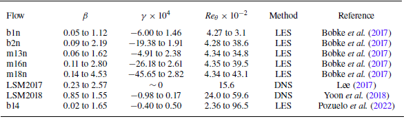
A brief description of eight flow fields, including Clauser pressure gradient
 $\beta$
, streamwise derivative of pressure gradient
 $\gamma$
as defined in (2.15), and momentum thickness Reynolds number
 $ \textit{Re}_\theta$
.

Another issue to discuss is that in APG TBLs, due to the velocity variation in the external flow, it is difficult to determine a well-defined ‘free-stream velocity’, thus the traditional
 $\delta _{99}$
is hard to apply. Therefore, in order to determine the nominal thickness
 $\delta$
, a diagnostic function is used here:
 \begin{align} f(y^*)=y^*\frac {\partial u^*}{\partial y^*}, \end{align}
and the outer edge of the boundary layer is defined as the location where
 $f(y^*)$
drops to
 $1/n$
of its second peak value. The method was proposed by Uzun & Malik (Reference Uzun and Malik2021), and was also adopted by Griffin, Fu & Moin (Reference Griffin, Fu and Moin2021). Conventionally,
 $n$
is taken as
 $2$
, so that this location corresponds to the definition of
 $\delta _{99}$
in ZPG TBLs approximately. However, in our model, it is desirable that the Reynolds shear stress
 $\tau _{R}^*$
to be close to zero at the outer edge of the boundary layer, requiring a slight expansion of the boundary layer thickness. Experiments have shown that a better definition is to use
 $\delta _{995}$
(Subrahmanyam et al. Reference Subrahmanyam, Cantwell and Alonso2022). Accordingly,
 $n$
is set to
 $5$
in the diagnostic function criterion.
3. Results
3.1. Database
The model is validated against eight direct numerical simulations (DNS) or LES flow fields, with the overall ranges of parameters presented in table 2, where
 $ \textit{Re}_\theta = {u_e \theta }/{\nu }$
denotes the momentum thickness Reynolds number. The flow fields are named as follows. The cases b1n, b2n and b14 correspond to TBLs subjected to relatively smooth, constant APGs, with Clauser parameters
 $\beta =1.0, 2.0, 1.4$
, respectively. The cases m13n, m16n and m18n denote flows in which the free-stream velocity follows a power-law distribution of the form
 $u_e(x)=C(x-x_0)^m$
, and
 $m=-0.13, -0.16, -0.18$
, respectively. The flows LSM2017 and LSM2018 simply refer to datasets used to analyse large-scale motions (LSMs) that were published in 2017 and 2018, respectively.
Among them, flow m18n has the strongest PG, and also the strongest local disequilibrating parameter
 $\gamma$
, while flow b14 has the highest Reynolds number. The tested flow fields cover a wide range of cases, with Clauser PG
 $\beta$
reaching maximum
 $4.53$
,
 $ \textit{Re}_\theta$
peaking at
 $9.65\times 10^3$
, and the non-dimensional second-order PG
 $\gamma$
ranging from
 $-4.57\times 10^{-3}$
to
 $2.82\times 10^{-4}$
. Flow data for LSM2017 are incomplete, therefore only the numerical results within its equilibrium region are used for validation.
The streamwise development of flow parameters is illustrated in figure 1. Here and throughout the rest of the paper, streamwise location
 $x$
is non-dimensionalised by the mean nominal boundary layer thickness
 $\delta _{99}$
within the computational domain,
 $\hat x=x/\langle \delta _{99}\rangle$
. As shown in figure 1(a), Clauser PG
 $\beta$
in all flow fields undergoes a process of first increasing and then decreasing. Correspondingly, in figure 1(b),
 $\gamma$
is first positive and then negative. Negative
 $\gamma$
can reach very large negative values, with its absolute magnitude far exceeding the maximum positive values. This is due to the smaller wall friction, and therefore smaller
 $u_\tau$
in the downstream region, which also indicates that downstream regions are more susceptible to local disequilibrating effects. Figures 1(c) and 1(d) illustrate that the streamwise evolution of the Reynolds number is relatively uniform and is not strongly related to variations of PG.
The markers in figure 1(a) indicate the locations of the profiles used for validation in § 3.3, which span a broad parameter space. However, limited validation exists for regions with
 $\gamma \gt 0$
, due to the fact that the flow fields in these regions may have relatively low Reynolds numbers, and be more susceptible to inflow conditions.
An overall description of seven flow fields along streamwise direction. The data are obtained directly through DNS or LES (Bobke et al. Reference Bobke, Vinuesa, Orlu and Schlatter2017; Yoon, Hwang & Sung Reference Yoon, Hwang and Sung2018; Pozuelo et al. Reference Pozuelo, Li, Schlatter and Vinuesa2022). The horizontal axis denotes the streamwise coordinate
 $\hat x=x/\langle \delta _{99}\rangle$
, where
 $x$
is non-dimensionalised by the nominal boundary layer thickness
 $\delta _{99}$
averaged over the computational domain. Plots show (a) Clauser PG
 $\beta$
, (b) streamwise derivative of PG
 $\gamma$
as defined in (2.15), with a zoomed-in view of the positive
 $\gamma$
region, (c) friction Reynolds number
 $ \textit{Re}_\tau$
, (d) momentum thickness Reynolds number
 $ \textit{Re}_\theta$
. The markers in (a) indicate the locations of the profiles used for validation in § 3.3: the green markers are tested in figure 3; the light blue markers are tested in figure 4; the red markers are tested in figure 5; the two blue triangle markers are tested in figure 7.

3.2. Verification of similarity
This subsection demonstrates that the new scaling method in § 2.1 effectively collapses the non-dimensional mixing length profiles (2.7), which play a fundamental role in the overall method.
We calculate
 $\lambda ^*$
directly from flow fields according to (2.5), and the results are shown in figure 2. Due to the relatively larger uncertainty of
 $\lambda ^*$
in the outer region, a one-dimensional Gaussian smoothing with window length 5 points (approximately
 $y^+=30{-}50$
in the outer region) is applied along the wall-normal direction. Here, the critical ratio
 $n$
of criterion (2.21) is set to
 $2$
. This is because at the outer edge of the boundary layer,
 $\partial u /\partial y$
is really small, leading to an ill-defined
 $\lambda ^*$
. Yet for the same reason, the magnitude of
 $\lambda ^*$
in these regions is not important, as
 $\partial u/\partial y$
is negligibly small, and the integration in this region has little impact on the mean profile of
 $u^*$
or
 $\tau ^*$
.
Twenty-five
 $\lambda ^*$
profiles in five flow fields are presented in figures 2(a) and 2(c). As shown in figure 2(a), in the inner region, even in the viscous sublayer where
 $y^+\lt 5$
, the new scaling method collapses all the mixing length profiles significantly better than the traditional friction-based scaling, which is shown in figure 2(b). In the outer region, the new scaling actually has the same form as the traditional friction-based scaling. As shown in figure 2(c), the horizontal axis is
 $\eta = y^*/Re_\tau ^*=y^+/Re_\tau =y/\delta$
, while the vertical axis is
 $\lambda ^*/Re_\tau ^*=\lambda ^+/Re_\tau ^+ = \lambda /\delta$
. All the profiles have similar growth trends, and their final stable values are closely aligned, showing obvious similarity in
 $\lambda ^*$
in different regions across different flow fields. In flow fields with stronger PG, such as flow m18n,
 $\lambda ^*$
in the outer region is less stable, but all the profiles end up at approximately
 $\lambda ^*/Re_\tau ^*= 0.08$
, which agrees well with our current model (2.7) at
 $y^* =Re_\tau ^*$
, as long as
 $ \textit{Re}_\tau ^* \gg a$
and
 $\ b\ll 1$
so that
 $\lambda ^*(Re_\tau ^*) \approx kb\, Re_\tau ^*$
, indicating that
 $kb\approx 0.08$
. This is also consistent with the optimal parameters in table 1.
Profiles of non-dimensional mixing length
 $\lambda ^*$
at different streamwise locations, in different flow fields. The data are obtained directly through DNS or LES (Bobke et al. Reference Bobke, Vinuesa, Orlu and Schlatter2017; Lee Reference Lee2017; Yoon et al. Reference Yoon, Hwang and Sung2018). The results have been processed with Gaussian smoothing, and the critical ratio
 $n$
in criterion (2.21) is set to
 $2$
. Within the same flow field, lines of lighter colour indicate locations further downstream. (a) Profiles under new inner scaling
 $\lambda ^*\sim y^*$
. (b) Profiles under traditional inner scaling
 $\lambda ^+\sim y^+$
. (c) Profiles under outer scaling
 $\lambda ^*/Re_\tau ^*\sim \eta$
(also
 $\lambda ^+/Re_\tau \sim \eta$
).

3.3. Verification of the estimation–correction model
In this subsection, it will be shown that the current estimation–correction model largely captures the shape of the profile and provides good predictive capability. To begin with,
 $\tau ^*$
from (2.17) can be decomposed into four parts, as shown in (3.1), namely
 $\tau _{0}^*, \ \tau _{\beta }^*, \tau _{e}^*,\ \tau _{\gamma }^*$
:
 \begin{align} \tau ^*=\tau _{0}^*+\tau _{\beta }^*+\tau _{e}^*+\tau _{\gamma }^*, \\[-28pt] \nonumber \end{align}
 \begin{align} \begin{cases} \tau _{0}^* = 1-G(y^*),\\[5pt]\displaystyle \tau _{\beta }^*= \frac {\beta }{1+\beta }\frac {1}{\delta _1^*}\left (\theta ^*(1-G(y^*))-\int _{y^*}^{Re_\tau ^*}\left (1-\frac {\widetilde u^{*2}}{u_e^{*2}}\right )\mathrm d y^*\right ),\\[12pt]\displaystyle \tau _{e}^*=\gamma \frac {\partial u_e^*}{u_e^*\,\partial \beta }\left (-\int _0^{y^*}\widetilde u^{*2}\,\mathrm dy^*+G(y^*)\int _0^{Re_\tau ^*}\widetilde u^{*2}\,\mathrm dy^*\right ),\\[12pt]\displaystyle \tau ^*_{\gamma }=\gamma \left ( \int _0^{y^*}\frac {\partial \widetilde u^{*2}}{\partial \beta }\,\mathrm d y^* -\widetilde u^*\int _0^{y^*}\frac {\partial \widetilde u^*}{\partial \beta }\,\mathrm d y^* -G(y^*)\right. \\[12pt]\qquad \left.\left ( \int _0^{Re_\tau ^*} \frac {\partial \widetilde u^{*2}}{\partial \beta }\, \mathrm d y^* -u_e^*\int _0^{Re_\tau ^*}\frac {\partial \widetilde u^*}{\partial \beta }\,\mathrm d y^* \right ) \right ). \end{cases} \\[0pt] \nonumber \end{align}
The first part,
 $\tau _{0}^*$
, is the shear stress introduced by the natural increase in the friction Reynolds number, independent of PG. It is also referred to as the Reynolds number effect, exactly the same form as (1.9), which is the balanced ZPG TBL case. From (2.17), it is easy to verify that
 $G(0)=0$
and
 $G(Re_\tau ^*)=1$
, yielding
 $\tau _{0}^*(0)=1$
and
 $\tau _{0}^*(Re_\tau ^*)=0$
, which is consistent with ZPG boundary conditions.
The second part,
 $\tau _{\beta }^*$
, demonstrates the effect of equilibrium PG on the entire profile, which is independent of non-equilibrium term
 $\gamma$
. The
 $(1+\beta )$
in the denominator is the result of scaling by
 $u_\beta ^{2} = u_\tau ^2 (1+\beta )$
, and actually, if scaled by the traditional viscous coordinate,
 $\tau _{\beta }^+$
is directly proportional to
 $\beta$
. At the boundary,
 $\tau _{\beta }^*(0)=-\beta /(1+\beta )$
and
 $\tau _{\beta }^*(Re_\tau ^*)=0$
. Together with
 $\tau _{0}^*$
, we have
 $\tau _{0}^*(0)+\tau _{\beta }^*(0)=1/(1+\beta )$
, which is consistent with wall conditions
 $\tau ^*(0)=\tau /(\rho u_\beta ^{2})=1/(1+\beta )$
.
The third part,
 $\tau _{e}^*$
, and the fourth part,
 $\tau _{\gamma }^*$
, are both proportional to
 $\gamma$
, which do not appear in the RANS equations, and these two parts are considered as the representation of first-order local disequilibrating effects. Also,
 $\tau _{e}^*$
is proportional to
 $\partial u_e^{*}/\partial \beta$
, therefore representing the coupling effect between PG and the outer flow development, while
 $\tau _{\gamma }^*$
is related to the integral of
 $\partial u^*/\partial \beta$
, which indicates the real local non-equilibrium effect induced by the varying PG. We have
 $\tau _{e}^*(0)=\tau _{e}^*(Re_\tau ^*)=\tau _{\gamma }^*(0)=\tau _{\gamma }^*(Re_\tau ^*)=0$
, indicating that the local disequilibrating effect only impacts regions far from the wall and far from the outer edge.
The validation results are shown in figures 3, 4 and 5. Among them, figure 3 shows the results of flow b1n, a rather mild APG flow, figure 4 shows the results of flow m16n, a moderate APG flow, and figure 5 shows the results of flow m18n, a rather strong APG flow. In all three figures, the four plots on the left represent the validation results of mean velocity profiles, where the black line shows reference data obtained directly from DNS or LES, the green line shows original model by Subrahmanyam et al. (Reference Subrahmanyam, Cantwell and Alonso2022), the blue dashed line denotes the estimation-step result
 $\widetilde u^*$
derived from (2.9), and the red line denotes the correction-step result
 $u^*$
derived from (2.19). Note that the parameters
 $(k,a,m,b,n)$
of the Subrahmanyam et al. (Reference Subrahmanyam, Cantwell and Alonso2022) model that we call here are the averages of the parameters given in their original paper (§ 6, table 5). The four plots on the right represent the validation results of total shear stress, where the black line still shows reference data from DNS or LES, the red line denotes the correction-step result
 $\tau ^*$
from (2.17), and the blue line denotes its decomposition
 $\tau _{0}^*+\tau _{\beta }^*$
from (3.1), which is the part independent of
 $\gamma$
. The discrepancy between the red line and the blue line is actually the first-order local disequilibrating effect that is proportional to
 $\gamma$
given by our estimation–correction model. All the figures are converted to the commonly used friction-based scaling.
Velocity and total shear stress profiles in flow field b1n (Bobke et al. Reference Bobke, Vinuesa, Orlu and Schlatter2017), showing different streamwise locations. (a,c,e,g) Profiles of mean velocity. The black solid line represents the reference LES data, the green solid line represents the original model by Subrahmanyam et al. (Reference Subrahmanyam, Cantwell and Alonso2022), the blue dashed line represents the estimation
 $\widetilde u^*$
obtained from (2.9), and the red solid line represents the correction
 $u^*$
obtained from (2.19). (b,d,f,h) Profiles of total shear stress. The black line represents the reference LES data, the red line represents the present model
 $\tau ^*$
from (2.17), and the blue line represents its decomposition
 $\tau _{0}^*+\tau _{\beta }^*$
from (3.1). All the quantities are converted to the commonly used friction-based scaling. The specific flow parameters are (a,b)
 $\hat x=21, \beta = 1.1, \gamma = -1.4\times 10^{-5}, Re_\tau = 448$
, (c,d)
 $\hat x=29, \beta = 1.0, \gamma = -1.2\times 10^{-5}, Re_\tau = 568$
, (e,f)
 $\hat x=41, \beta = 0.9, \gamma = -0.9\times 10^{-5}, Re_\tau = 716$
, (g,h)
 $\hat x=52, \beta = 0.6, \gamma = -14.7\times 10^{-5}, Re_\tau = 851$
.

Velocity and total shear stress profiles in flow field m16n (Bobke et al. Reference Bobke, Vinuesa, Orlu and Schlatter2017), showing different streamwise locations. The legend follows the same convention as in figure 3. Note that in (b), the blue line and the red line are so close that they almost collapse. The specific flow parameters are (a,b)
 $\hat x=17, \beta = 2.8, \gamma = -1.1\times 10^{-5}, Re_\tau = 422$
, (c,d)
 $\hat x=23, \beta = 2.5, \gamma = -4.0\times 10^{-5}, Re_\tau = 539$
, (e,f)
 $\hat x=32, \beta = 2.1, \gamma = -4.8\times 10^{-5}, Re_\tau = 704$
, (g,h)
 $\hat x=41, \beta = 0.9, \gamma = -50.0\times 10^{-5}, Re_\tau = 861$
.

Velocity and total shear stress profiles in flow field m18n (Bobke et al. Reference Bobke, Vinuesa, Orlu and Schlatter2017), showing different streamwise locations. The legend follows the same convention as in figure 3. Note that in (d), the blue line and the red line are so close that they almost collapse. The specific flow parameters are (a,b)
 $\hat x=15, \beta = 4.1, \gamma = 14.6\times 10^{-5}, Re_\tau = 402$
, (c,d)
 $\hat x=21, \beta = 4.5, \gamma = -2.4\times 10^{-5}, Re_\tau = 503$
, (e,f)
 $\hat x=30, \beta = 3.5, \gamma = -15.9\times 10^{-5}, Re_\tau = 669$
, (g,h)
 $\hat x=38, \beta = 0.8, \gamma = -95.4\times 10^{-5}, Re_\tau = 858$
.

In figures 3(a,c,e,g), it can be seen that the prediction of the correction-step result
 $u^*$
is highly accurate at all locations, generally superior to the original model, and far superior to the estimation-step result
 $\widetilde u^*$
. Three models all behave well in the inner region. In the buffer region, the original model is larger, while
 $\widetilde u^*$
is smaller, and in the wake region, the original model and
 $\widetilde u^*$
are both smaller than the LES result. This is because the initial estimation
 $\widetilde \tau ^*$
in (2.8), which is obtained based on channel flow results, is a straight line, whereas in an APG TBL, real shear stress is a concave function that exceeds the initial
 $\widetilde \tau ^*$
at all points except the boundaries, as shown in figures 3(b,d,f,h). As a result, the Subrahmanyam et al. (Reference Subrahmanyam, Cantwell and Alonso2022) original model and
 $\widetilde u^*$
which are based on
 $\widetilde \tau ^*$
both underestimate. Meanwhile, in order to balance this outer-region error, based on the min-square-error criterion, the original model forcibly obtains the optimal parameters, resulting in the non-physical overestimation in the buffer region. In short, the advantage of our model
 $u^*$
is significant. However, the accuracy of
 $u^*$
on flow b1n is within expectation, as the tunable parameters
 $(k,a,m,b,n)$
of our current model were determined based on this dataset.
In figures 3(b,d,f,h), it can be seen that the correction-step prediction
 $\tau ^*$
is also very close to the LES results. In the inner region, at locations with smaller
 $|\gamma |$
where the boundary layer is in near-equilibrium state, such as figures 3(d,f),
 $\tau ^*$
agrees better with LES data compared to figures 3(b,h), where the local non-equilibrium effect is rather significant. In the outer region, none of the profiles matches the data well. One of the key reasons for this is that although we have set the critical ratio
 $n = 5$
in criterion (2.21) to ensure that the shear stress tends to zero outside the boundary layer, it remains at approximately
 $0.1$
as shown by the black lines. However, in theoretical analysis,
 $\tau ^*(Re_\tau ^*)$
should accurately be zero. Furthermore, shown by the discrepancy between the red and blue lines in figures 3(b,d,f,h), the term
 $\tau _{e}^* + \tau _{\gamma }^*$
that indicates the local disequilibrating effect always adjusts
 $\tau ^*$
to the correct direction. In particular, in figure 3(h), the effect of the streamwise derivative of PG on
 $\tau ^*$
profile is clearly visible.
Except for flow field b1n in figure 3, all the results shown in other figures are part of the validation set rather than the calibration set.
In figure 4, the results are generally consistent with those in figure 3. As shown in figures 4(a,c,e,g), the correction-step result
 $u^*$
maintains high accuracy across all locations, and its improvement over the estimation
 $\widetilde u^*$
and the original model is even more evident. In figures 4(b,d,f,h), although the final result
 $\tau ^*$
exhibits some numerical deviation, it still captures the overall trend of the LES data well.
Figure 5 still presents almost the same results as figures 3 and 4. In figures 5(a,c,e,g), the prediction of
 $u^*$
is still accurate at all locations, far better than
 $\widetilde u^*$
and the original model. In figures 5(b,d,f,h),
 $\tau ^*$
still captures the general shape and trend of the LES data, despite exhibiting non-negligible deviations in magnitude. In general, for flow m18n, the prediction deviates more from LES data compared to flow b1n or m16n. This can be attributed partially to the stronger APG effect, which induces more significant local non-equilibrium effects. However, as a validation set, the observed error of
 $u^*$
in figures 5(e,g) remains within an acceptable range.
In figures 5(b,d,f,h), the local disequilibrating effect terms
 $\tau _{e}^*$
and
 $\tau _{\gamma }^*$
still adjust
 $\tau ^*$
to the correct direction, and especially in figure 5(h) where
 $|\gamma |$
is considerably large, the local disequilibrating effect plays a significantly vital role in the total shear stress profile. However, the current stress profile predictions still leave room for improvement. One possible reason for the overprediction in figures 5(b,d) may be the relative low Reynolds number(
 $ \textit{Re}_\tau =402,503$
), which leads to incomplete turbulence development, and consequently an overestimation of the Reynolds stress
 $\langle u^\prime \,v^\prime\rangle$
.
To avoid excessive discussion, the validation results for other flow fields are not presented in such detail. Instead, figure 6 shows the comparison of the cumulative relative error of velocity prediction given by the original model and the current model. The relative error is defined as
 \begin{align} \mathrm{Error} = \frac {\int _0^{Re_\tau }|u^+-u_0^+|\,\mathrm{d}y^+}{\int _0^{Re_\tau } u_0^+\,\mathrm{d}y^+}, \end{align}
where
 $u^+$
is the prediction value, and
 $u_0^+$
is the true value given by DNS/LES. As shown by figure 6, our model performs generally better than the original model. In flow fields where
 $\beta$
is relatively large or varies rapidly, such as m18n, m16n and b2n, the predictive accuracy of our model is significantly higher than that of the original model. When
 $\beta$
is small, our model still performs slightly better than the original model, such as in flows b1n and m13n. However, at higher Reynolds numbers, the prediction error of our model increases noticeably and becomes comparable to that of the original model, such as in flow b14. A possible reason is that our calibration dataset is based on flow field b1n, which corresponds to a relatively low Reynolds number. This suggests a possible Reynolds number dependence of the model parameters.
Cumulative relative error of velocity prediction. The crosses show the prediction error given by the original model of Subrahmanyam et al. (Reference Subrahmanyam, Cantwell and Alonso2022), while the dots show the prediction error given by the current model. The error is given by (3.3).

To intuitively demonstrate the role of the local disequilibrating effect, we extract one profile each from the flow fields m13n and m18n. These two profiles share the same
 $ \textit{Re}_\tau$
and
 $\beta$
, but differ significantly in
 $\gamma$
, with ratio approximately 9. The streamwise locations of the selected profiles are indicated by the blue triangle markers in figure 1(a). As shown by figures 7(a,b), it is evident that both the velocity and shear stress distributions differ significantly between the two profiles. Encouragingly, our model, through the correction involving
 $\gamma$
, successfully captures the differences between the two profiles.
As shown by figures 7(a,b), a large negative value of
 $\gamma$
leads to reduced velocities in the near-wall region, increased velocities in the outer region, and an overall increase in total shear stress. This is because a larger absolute value of
 $\gamma$
indicates a more rapid variation of the PG, while the velocity and stress profiles (especially the stress profile) cannot adjust to such rapid changes, exhibiting a lag, as described by Bobke et al. (Reference Bobke, Vinuesa, Orlu and Schlatter2017). Regarding the current cases, if the cases with small
 $|\gamma |$
are considered approximately in equilibrium, then the cases with larger negative
 $\gamma$
largely reflect the flow under a stronger PG. Therefore, both the stress and velocity profiles are closer to those observed at higher
 $\beta$
. As is well known, a strong APG leads to reduced velocities in the near-wall region, increased velocities in the outer region, and an overall increase in total shear stress; thus a large negative
 $\gamma$
also produces these effects. However, as stated above, since only local disequilibrating effects are obtained, the results remain subject to non-negligible deviations.
Two profiles extracted from flow fields m13n and m18n (Bobke et al. Reference Bobke, Vinuesa, Orlu and Schlatter2017), with the same
 $\beta$
and
 $ \textit{Re}_\tau$
, but different
 $\gamma$
: (a) mean velocity profiles, and (b) total shear stress profiles. The blue lines indicate flow m13n,
 $\hat {x} = 48$
,
 $\beta = 0.77$
,
 $\gamma = -11.1 \times 10^{-5}$
,
 $ \textit{Re}_\tau = 862$
. The red lines indicate flow m18n,
 $\hat {x} = 37.8$
,
 $\beta = 0.77$
,
 $\gamma = -97.6 \times 10^{-5}$
,
 $ \textit{Re}_\tau = 861$
.

Finally, a detailed analysis was performed on the contributions of each decomposed term of
 $\tau ^*$
in (3.1), based on the data calculated at six different streamwise locations of flow m18n. The corresponding results are shown in figure 8.
Figure 8(a) shows the profile of
 $\tau _{0}^*$
, which is the part that is completely independent of PG. Its profile is similar to the ZPG TBL case, or even the straight-line profile of the channel flow case. This explains why the channel flow shear stress profile can be used directly in ZPG TBLs, and can be used as the initial estimation in our model. All six profiles start from
 $\tau _{0}^*(0)=1$
at the wall, and monotonically decrease to
 $\tau _{0}^*(Re_\tau ^*)=0$
at the outer edge. The profiles are highly similar.
Figure 8(b) shows the profile of
 $\tau _{\beta }^*$
, which is the part that is directly proportional to
 $\beta$
and independent of non-equilibrium effect
 $\gamma$
. All six profiles start from
 $\tau _{\beta }^*(0)=-\beta /(1+\beta )$
, reach a peak at approximately
 $0{-}1$
, and finally drop to zero at the outer edge. The peak value gradually decreases along the streamwise direction. Despite the difference in
 $\beta$
, the six profiles still exhibit strong similarity.
Figures 8(c,d) show the profiles of
 $\tau _{e}^*$
and
 $\tau _{\gamma }^*$
, respectively, which are the parts that are directly proportional to
 $\gamma$
. These two terms are almost equal in magnitude but opposite in sign, achieving a delicate balance between the interaction of PG with outer flow development, and the local pressure non-equilibrium effect. All the profiles vary from zero back to zero, undergoing a transition from positive to negative, or the opposite, depending on the sign of
 $\gamma$
.
Figures 8(e,f) show the profile of
 $\tau _{0}^* +\tau _{\beta }^*$
, which is the part that is independent of
 $\gamma$
, and the profile of
 $\tau _{e}^*+\tau _{\gamma }^*$
, which is the part that is proportional to
 $\gamma$
and shows a first-order local disequilibrating effect. A comparison between the two plots reveals that the non-history effect component of the total stress is relatively consistent across all profiles, while the local-disequilibrating-effect term varies sensitively with the magnitude of
 $\gamma$
. The local disequilibrating effect peaks at approximately
 $1.3$
, contributing approximately half of the total stress.
From the analysis of figure 8, we can see that the height and location of the shear stress peak are determined by the
 $\tau _\beta ^*$
term, because
 $\tau _0^*$
does not exhibit a peak, while the other two terms are very small in magnitude most of the time. Therefore, the mismatch of total shear stress profiles shown in figures 3(b,d,f,h), 4(b,d,f,h) and 5(b,d,f,h), and also the mismatch of the peak location shown in figure 7(b), are probably caused by
 $\tau _\beta ^*$
. Unfortunately, due to the lack of true values, further analysis is challenging. We will continue to devote our efforts to investigating this issue.
Profiles of the components of the correction-step result
 $\tau ^*$
, calculated at different streamwise locations of flow field m18n (Bobke et al. Reference Bobke, Vinuesa, Orlu and Schlatter2017): (a,b,c,d) contributions of
 $\tau _{0}^*,\tau _{\beta }^*,\tau _{e}^*,\tau _{\gamma }^*$
, respectively; (e)
 $\tau _{0}^* +\tau _{\beta }^*$
; (f)
 $\tau _{e}^*+\tau _{\gamma }^*$
. All the quantities are converted to the commonly used friction-based scaling.

4. Discussion and conclusion
In this study, a general modelling framework for APG TBLs is developed that, for the first time, explicitly incorporates the local disequilibrating effect through local flow parameters. A modified set of non-dimensional scales successfully collapses the mixing length profile across a wide range of flow fields in both the inner region and the outer region. The streamwise derivative of PG,
 $\gamma$
, is naturally introduced in the estimation–correction method between
 $u$
and
 $\tau$
, which can represent the local disequilibrating effect, significantly enhancing the predictive capability for both mean velocity and total shear stress profiles.
The correction-step result
 $\tau ^*$
is decomposed into four parts, corresponding respectively to Reynolds number effects, equilibrium PG effects, the coupling between free-stream velocity and PG, and local non-equilibrium PG effects. The latter two are considered first-order local disequilibrating effects, which typically offset each other, but in downstream regions their combined effect becomes significant, accounting for nearly half of the total shear stress.
The model is validated against eight DNS or LES datasets, covering a wide range of Reynolds numbers and PGs. Across all cases, the model maintains high predictive accuracy, outperforms previous methods, and clearly demonstrates the impact of the local disequilibrating effect on the boundary layer profiles.
In fact, the estimation–correction method can be further repeated, allowing for introducing higher-order streamwise derivatives of PG into the profiles of velocity or shear stress. After closure via the mixing-length model, the original RANS equations contain only two unknowns,
 $u$
and
 $v$
, while in the iterative estimation–correction method, we may iteratively solve for
 $u^*$
and
 $\tau ^*$
, which also constitutes a system with two unknowns. This guarantees that this iterative estimation–correction model can make full use of the information given by the governing equations. In each round of iteration, first,
 $u^{*}_{n+1}$
is obtained given
 $\tau ^{*}_n$
. This process can be completed directly through (2.6) without adding computational complexity. Then, just as in the current model, by converting the streamwise derivatives into the derivatives of other flow parameters, and then sequentially expanding the terms in RANS equations and the continuity equation, we can solve for
 $\tau _{n+1}^*$
according to
 $u^*$
as an explicit function. The iteration can be done systematically, introducing higher-order correction, and the terms can be regarded as higher-order local disequilibrating effects. However, complexity grows rapidly as further expansion is conducted.
There also remain several limitations. Most notably, the predictions of the shear stress profiles are still not sufficiently accurate. One of the issues is that the predicted shear stress remains non-zero at the outer edge of the boundary layer, which contradicts the theoretical assumptions. Future work may address this by redefining the boundary layer thickness
 $\delta$
or manually adding a correction term at the edge.
Additionally, although the model has been tested for cases with
 $\beta$
up to 4.53, it is not applicable to profiles near boundary layer separation, which is the area of great practical interest. One critical issue is that near separation, the wall friction velocity
 $u_\tau$
approaches zero, rendering all wall-based scalings invalid.
In summary, our model accurately predicts the mean velocity and total shear stress profiles in APG TBLs, and explicitly incorporates the local disequilibrating effect through local parameters. This not only deepens the understanding of the underlying physics of APG TBLs, but also offers new ideas and insights for improving turbulence modelling and closure strategies for the RANS equations. Furthermore, the present work may provide a theoretical foundation for the development of wall models in LES under complex boundary conditions.
Acknowledgements
The authors would like to express their appreciation to the programme of Open Research for Innovation Challenges (ORIC), supported by the Tsien Excellence in Engineering Programme (TEEP), Tsinghua University.
Funding
This work is supported by the National Natural Science Foundation of China (under grant nos 12272205 and 12388101).
Declaration of interests
The authors report no conflict of interest.