1.1 Information theory and computational linguistics

Information theory (IT) (Shannon Reference Shannon1948) is pervasive within computational linguistics (CL), and the relationship between the two has a long history. Chomsky's well-known theory of formal grammars (Chomsky Reference Chomsky1956, Reference Chomsky and Halle1959) (applicable to generative grammar in phonology, morphology, and syntax) appeared, significantly, in publications on IT. Even before this, Cherry, Halle and Jakobson (Reference Cherry, Halle and Jakobson1953) explicitly cast phonological classification in an information-theoretic light, and this tradition was continued in The Sound Pattern of Russian (Halle Reference Halle1959) and The Sound Pattern of English (Chomsky and Halle Reference Chomsky and Halle1968).

The recognition that information-theoretic principles have importance in CL has, if anything, been renewed in recent years. In phonology Broe (Reference Broe1996) describes the use of IT as a measure for phoneme classification and recognition systems. In a paper which has relevance to syntax, Brown et al. (Reference Brown, deSouza, Mercer, Della Pietra and Lai1992) pointed to the fact that mutual information (or, to be more precise, pointwise mutual information) can be used as a heuristic to discover word collocations in an unsupervised learning system. A similar approach, also using pointwise mutual information, was taken by Lin (Reference Lin1999). Essentially the same technique was used by Kashioka et al. (Reference Kashioka, Kawata, Kinjo, Finch and Black1998) for unsupervised morphological analysis of Japanese, although in this case the ‘collocations’ are of characters rather than words. Other examples of the use of pointwise mutual information include Bullinaria and Levy (Reference Bullinaria and Levy2007) and Recchia and Jones (Reference Recchia and Jones2009).

Like Kashioka et al. (Reference Kashioka, Kawata, Kinjo, Finch and Black1998), Goldsmith (Reference Goldsmith2001) used pointwise mutual information as a heuristic to identify morphemes (one of many elements in his approach), but more importantly showed that the applicability of IT to morphology was very general. Goldsmith (Reference Goldsmith2001) showed that IT, and specifically the Minimum Description Length (MDL) model (Rissanen Reference Rissanen1989), could be used to evaluate one theory of morphology against another. In Section 2.3, we return to a more in-depth consideration of IT-based morphological analysis of the sort described by Goldsmith (Reference Goldsmith2001), and the role that it can play in information retrieval (IR).

Perhaps one of CL's greatest recent successes is Statistical Machine Translation (SMT) (Brown et al. Reference Brown, Della Pietra, Della Pietra and Mercer1994). At the heart of SMT, again, is IT. Brown et al. (Reference Brown, Della Pietra, Della Pietra and Mercer1994) make this link explicit by referring to the earlier work of Weaver (Reference Weaver1955) in communication theory, and to the centrality of Bayes' theorem in machine translation. As Brown et al. (Reference Brown, Della Pietra, Della Pietra and Mercer1994) make clear, a key objective in SMT is to align words in one language with those in another from a parallel corpus. In effect, Bayes' theorem is used to select pairings of words that maximize mutual information in a way very similar to that described (in a different context) in Brown et al. (Reference Brown, deSouza, Mercer, Della Pietra and Lai1992) and Kashioka et al. (Reference Kashioka, Kawata, Kinjo, Finch and Black1998).

1.2 Information theory (IT) and information retrieval (IR)

From the outset, IR has had more utilitarian goals than CL. A common theme in the history of IR has been the need to catalog information so that it can later be accessed efficiently. In the 1940s, the US military confronted this problem with documents captured from the Germans; in the 1950s, the US again looked to IR as a way to automate search of scientific literature produced in the USSR; and of course from the 1990 onwards the world wide web has presented a challenge vastly larger in scale than any of the previous ones. An essential feature of IR is its interdisciplinary nature, combining computer science, mathematics, library science, and statistics. It would probably be fair to say that IT (not to be confused with information science) has been at most incidental in the development of IR.Footnote ¹

Nevertheless, IT has not passed IR completely. One of the most popular term-weighting schemes in IR today is the ‘log-entropy’ weighting scheme (Dumais Reference Dumais1991), which we shall discuss more fully in Section 2. Under this scheme, the importance of a word in a document is estimated from the product of a ‘local weight’ and a ‘global weight’. The global weight is derived from (inversely related to) the entropy of the term across the whole corpus. In IT, entropy is in fact a measure of how much noise (or conversely, information) is contained in an event: the higher the entropy (and, correspondingly, the lower the global weight), the less information the event contains. Clearly, the success and enduring popularity of the log-entropy weighting scheme are related to the fact that entropy is a realistic estimate of how much linguistic information is contained in a word.

Another important link between IT and IR has to do with signal processing. Key considerations in signal processing are the compression of information, separation of information from noise, and feature extraction. Linear algebra offers a widely used tool to achieve these goals: singular value decomposition (SVD) (Eckart and Young Reference Eckart and Young1936; see also Golub and van Loan Reference Golub and Van Loan1996). The original application of SVD to text retrieval is generally considered to be Latent Semantic Analysis (Deerwester et al. Reference Deerwester, Dumais, Landauer, Furnas and Harshman1990), which approximates a large, sparse term-by-document matrix by decomposing it into smaller and dense matrices that map the terms and documents to ‘concepts’. As SVD is guaranteed to find the best rank-k approximation (in a least-squares sense) to a rank-n matrix, where k < n, one can think of Latent Semantic Analysis (LSA) as distilling the information in a set of terms and documents into a more compact representation and finding the set of concepts that best describe the terms and documents in that smaller space. It is also claimed (Deerwester et al. Reference Deerwester, Dumais, Landauer, Furnas and Harshman1990) that LSA reduces the inherent ‘noisiness’ of language by placing documents in concept space rather than term space: because two distinct terms (or types) may have very similar meaning, a keyword search may retrieve documents with one term but not the other, but this problem is sidestepped (so the argument goes) when the search is based on concept vectors.

The remainder of this article is organized as follows. In Section 2 we scrutinize a number of assumptions that are commonly made in IR. The areas we consider boil down to the following: weighting schemes, what constitute ‘terms’ and ‘documents’, and mechanisms for the representation of linguistic entities in vector space. By looking at what IT might have to say on each of the issues considered, we raise questions about whether IR, as it is commonly practiced, in effect accepts ‘satisficing’ solutions – those which work adequately, but are perhaps nonoptimal from a theoretical and empirical perspective.

In Section 3 we set out a coherent IR framework that deals with these areas in a principled way. In each case, we can trace the proposed innovations to parallels in the CL literature, showing that there need be no conflict between insights from generative linguistics and a fully unsupervised, statistics-based, ‘real-world’ approach to IR – and moreover one which can be applied more or less to any language.

An empirical comparison of different variants on our approach (as applied to a particular multilingual dataset) and the ‘standard’ approach to IR is set out in Section 4.Footnote ² It will become clear that in every case, a theoretical improvement is accompanied by an empirical improvement. Overall, however, a clear picture emerges: A right understanding of IT, and its relationships to natural language, is essential in crafting the best possible approach to IR. We discuss this in Section 5, at the same time pointing to other areas in which the application of some other ideas from IT could benefit IR still further.

2.1 Background on IR

In this section, we give a brief overview of relevant concepts in IR. For a more detailed description on any point, see Baeza-Yates and Ribeiro-Neto (Reference Baeza-Yates and Ribeiro-Neto1999).

Most of IR dealing with text (specifically, IR based on the vector space model) is based on the insight that terms and documents can be arranged into a matrix format, where each row stands for a term i, each column for a document j, and the numerical entry in cell (i, j) is the number of times i appears in j. For now we can think of a term as any text delimited by non-word characters (for the latter, there is a standard definition in the regular expressions language). The matrix we form says nothing about the ordering of terms in documents, which is why the approach is sometimes referred to as a ‘bag-of-words’ approach.

The existence of the term-by-document matrix implies the existence of document vectors (the columns in the matrix) and term vectors (the rows). In the case of the document vectors, the terms can be thought of as unordered features or attributes, and the numerical entries in the vector, as attribute-values. Similarly, the term vector also has attributes (the documents) and attribute-values: in effect, the term is defined by the documents in which it occurs. In order to compute the similarity of a term to another term, or a document to another document, we may simply find the cosine of the angle between the two respective vectors. As this general approach to text retrieval treats documents and terms as vectors, it is often described as the vector space model (VSM).

In practice, there are many transformations applied to term-by-document matrices and many uses to which they can be put, but the above outline holds broadly true for most text retrieval. We will discuss and evaluate some of these transformations from an IT perspective in the following sections.

2.2 Weighting schemes and pointwise mutual information

In this section, we examine the most common weighting scheme (log-entropy) and suggest what we consider a more principled approach, namely, pointwise mutual information.

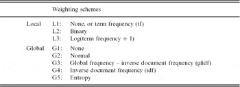
Standard weighting schemes. As Dumais (Reference Dumais1991) points out, a ‘common and usually effective [method] for improving retrieval performance'’ is to set (i, j) in the term-by-document matrix equal not to the number of times i appear in j (the raw frequency), but rather to use a term weighting scheme (Sparck Jones Reference Sparck Jones1972; Salton and Buckley Reference Salton and Buckley1988; Salton Reference Salton1991). Terms are usually weighted according to a local and/or global weight. Common weightings listed by Dumais (Reference Dumais1991) are shown in Table 1. Further weighting schemes are listed in Chisholm and Kolda (Reference Chisholm and Kolda1999).

Table 1.

Term–document weighting schemes

In principle, the local and global weightings can be combined together however one wishes, so with the options in Table 1, there are fifteen possible combinations. When combined, the local weighted value is multiplied by the global weight: as an example, the expression for log-entropy weighting (L3–G5) is as follows:

1. (1)

where w(i, j) is the ‘transformed’ (or weighted) frequency of term i in document j, f(i, j) is the raw frequency, N is the number of documents in the corpus, and p(i, j′) is the probabilityFootnote ³ that a given occurrence of i is in document j′, or f(i, j′) divided by the total frequency of i in the corpus.

Dumais (Reference Dumais1991) actually tests six local/global combinations: L1 together with each of the five possibilities for G, and L3–G5, or log-entropy. It is probably in large part due to her work, which demonstrates the superiority of log-entropy over the others that log-entropy weighting is perhaps the most popular weighting scheme to date. This is attested to by the ubiquity of log-entropy weighting options in commonly used commercial-off-the-shelf text mining software, such as SAS and Statistica.

Relationship of term weighting and IT. It is important to note the links between some of these weighting options and IT. One of these is alluded to by Dumais herself, which states that ‘entropy is based on information-theoretic ideas and is the most sophisticated weighting scheme'’ (Dumais Reference Dumais1991: 233). As already mentioned, entropy is a measure of noise. In (1) above, −∑_j′ p(i, j′) log p(i, j′) is the element that expresses the term entropy. Here, the term is treated as a random variable with a probability distribution; the observed frequencies in the corpus allow us to estimate that probability distribution. Another way of thinking of entropy is as the total expected value of the log-probabilities. For a term that occurs with equal frequency (and therefore probability) in all N documents – an unlikely scenario in natural language – the entropy is equal to −log(1 / N), or log(N), and it will be clear from (1) that the global weight will be 0, as will w(i, j). For the hapax legomena of the corpus (lexical items that occur in only one place), the entropy is 0 and the global weight is 1.

As we have said, Dumais noted the connection between log-entropy and IT, but in fact both L3 and G4 also have a basis in IT. We consider each of these in turn.

In the case of L3, or log(term frequency + 1), there is a clear comparison with log(term probability). (The purpose of adding 1 in L3 is simply to avoid cases where the log of zero would have to be computed.) Clearly, for any given term, term frequency and term probability are, by definition, proportional to one another. It also follows that log(frequency) and log(probability) are related as follows:

1. (2)

where f(i) is the total frequency of term i in the corpus. As already mentioned, log-probability is one element in the term's entropy. Note that (2) is an approximation because strictly speaking the probability is estimated from surface data.

For G4 (idf), there is a similar connection to IT. Idf is expressed as follows:

1. (3)

where df(i) is the number of documents in which term i occurs. Here too we are dealing with a log-probability: term i is now treated as an event that either occurs or does not occur in a given document. The expression df(i) / N is the probability of that event; and −log(df(i) / N), or equivalently log(N / df(i)), is the negation of the event's log-probability.

It is worth stopping for a moment to consider why log frequency (or probability) is used rather than raw frequency in VSM approaches. The usual way of looking at this is by reference to the Zipfian nature of word distributions. We do not dispute the validity of this perspective, but would point out that it is important to use a log scale in VSM approaches because of the way we manipulate vectors and matrices: a matrix multiplication involves the addition of pointwise products. Deerwester et al. (Reference Deerwester, Dumais, Landauer, Furnas and Harshman1990) mention that queries and documents can be considered as weighted sums of their component term vectors; Landauer, Foltz and Laham (Reference Landauer, Foltz and Laham1998: 6) put it another way, stating that ‘LSA represents the meaning of a passage as a kind of average of the meaning of the words it contains'’. From a probabilistic point of view, the idea of summing (or averaging) semantic term vectors in this way is closely related to the idea in CL (for example, in Naïve Bayes classification) that the probability of a document is the product of the probabilities of the terms it contains (assuming that the terms are independent). As is well known, one convenient way of obtaining a product of probabilities is to obtain the sum of the log probabilities. This brings us full circle to the appropriateness of log probabilities or frequencies in the VSM. As matrix multiplication is additive in the way discussed above, we effectively have no choice but to work in log space when using VSM approaches to IR, a point which is generally left unexplained in the literature.Footnote ⁴

Pointwise mutual information. Though these weighting schemes have a clear foundation in IT, and their widespread use attests to their effectiveness, they have some aspects that are theoretically problematic. We have explained the need to use the log-frequency rather than the raw frequency, showing that this has a basis in probability theory, which is related to IT. In addition, we can say that the global weight factor should be closer to 1 for low-entropy terms and closer to 0 for high-entropy terms. But what of the interplay between these two components? Why should they be multiplied together (other than that this is what gives the best empirical results)? Why not raise the global weight to some power α, as suggested by Bader and Chew (Reference Bader and Chew2008)?

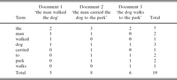
We can sidestep these issues by proposing an alternative weighting scheme based on pointwise mutual-information (PMI). This system is computationally and theoretically simpler than log-entropy, and we believe its elegance makes it easier to explain from the standpoint of IT. Here, the weighted frequency w(i, j) is simply the PMI between the term i and the document j. To illustrate, we consider the hypothetical term-by-document matrix in Table 2.

Table 2.

Hypothetical term-by-document matrix

PMI weighting treats each token in the corpus as an event (as do other weighting schemes), and the terms and documents both as variables. The probability of a term p(i) is simply i's prior probability: the probability that, given any token selected at random from the corpus, it is i. Thus, based on Table 2, p(‘the’) is 7/19, or about 0.368. Likewise, the probability of a document p(j) is the probability that a given token selected at random came from j. For example, the probability of document 1 above is 5/19 or about 0.263. The joint probability p(i, j) is the probability that the randomly selected token both is the term i, and it came from j. Thus, p(‘the’, doc1) here would be 2/19, or about 0.105. We assign to w(i, j) the PMI of a term i and a document j, which is familiar from other contexts in CL (e.g. Brown et al. Reference Brown, deSouza, Mercer, Della Pietra and Lai1992; Goldsmith Reference Goldsmith2001), as follows:

1. (4)

Advantages of PMI. As can also be seen from (4) (through the application of Bayes's theorem), we may equivalently say that w(i, j) is the log of (P1 / P2), where P1 is the probability of i occurring in j, and P2 is the probability of i occurring in the corpus as a whole. Note that w(i, j) is negative in cases where P1 < P2, and is maximized when i occurs only in j. By using PMI weighting, we avoid having to deal with separate local and global weights and the interaction between them, the information-theoretic rationale for the weighting scheme is very clear, and we bring it much more into line with other aspects of CL. Though PMI weighting has been proposed before also (e.g. Matveeva et al. Reference Matveeva, Levow, Farahat and Royer2005), in all previous cases of which we are aware, PMI is applied to pairs of terms and not to term–document pairs, as we propose here.

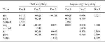
We can compare PMI and log-entropy weighting practically by examining Table 3, which is intended as an illustration rather than a formal proof of the superiority of PMI. Note for example that for Doc1, the ranking of terms by weight is very similar, but, in contrast to mutual-information, log-entropy ranks ‘the’ higher than ‘dog’ in Doc1. To our linguistic intuition, the ranking for Doc1 under mutual-information seems preferable to that under log-entropy. It also seems reasonable that ‘dog’ should have some weight, rather than the uniform weight of zero assigned by log-entropy. However, we do not stop at an intuitive evaluation; we will compare the two methods empirically. For this, we leave further discussion to Section 4.

Table 3.

Comparison of mutual-information and log-entropy weighting

One other point that recommends PMI weighting above log-entropy weighting is that extending the former from two-dimensional matrices, such as that in Table 2, to tensors (n-way arrays; see Section 2.6 for examples in text analysis) appears to be straightforward. It is not clear how or whether this would be true of log-entropy weighting. Adaptation of PMI weighting (see (4) above) to tensors could be as simple as (5), known in IT as total correlation,

1. (5)

In summary, we suggest that the reason PMI may be superior to log-entropy as a weighting scheme is that it has a clear theoretical basis in IT, avoids the question of how to combine local and global weights, is extensible to more than two dimensions, and provides what seem to be somewhat more reasonable linguistic results.

2.3 Defining ‘terms’

In this section, we examine more closely the definition of ‘term’ and suggest that the use of morphological analysis from CL is preferable to the standard stemming approach. We further suggest that MDL provides an appropriate nonsupervised, non-language-specific IT approach to morphological analysis.

As mentioned above, defining the term can be straightforward, and, for the most part, non-language-specific. In fact, the regular expressions language can do the job for us, because it pre-defines which characters are ‘word’ characters and which are ‘non-word’ characters: terms can be any strings delimited by non-word characters.

This approach has a shortcoming, however, that will be obvious from the examination of Table 2. Clearly, ‘walked’ and ‘walks’ are linguistically related. But the common stem ‘walk’ may not be one of the terms in the term-by-document matrix, if the string ‘walk’ is not bounded by non-word characters anywhere in the corpus. At the same time, the term-by-document matrix fails to encode the linguistic relationship between ‘walks’ and ‘walked’; there is a row corresponding to each term, but the matrix would look no different (numerically) if ‘walks’ were replaced by ‘runs’; accordingly, whether the term is ‘walks’ or ‘runs’, it is essentially of no consequence in wordform-based IR.

This shortcoming is recognized and addressed to some degree by a standard technique in IR: stemming (Lovins Reference Lovins1968). There have been many variants on approaches to stemming, including using stem-lookup tables, suffix- or affix-stripping (requiring only tables of affixes), and lemmatization. Interestingly, many current approaches to stemming are computationally quite complex and rule-driven, and may involve the use of lookup tables (e.g. Tomlinson Reference Tomlinson2004). These approaches therefore tend to introduce an undesirable dependence on a priori information. As both rules and lookup tables are generally developed by hand, they may be costly to develop. Regardless of how stemming is performed, the goal is almost always to reduce terms to a set of common stems: taking Table 2 as an example, the rows for ‘walks’ and ‘walked’ would be subsumed into a single row for ‘walk’, allowing a statistical similarity to emerge between documents 1 and 3 where it would otherwise have been missed.

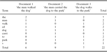
From a linguistic point of view, stemming may be an improvement on no stemming, but it does not tell the whole story. With rows in the term-by-document matrix only for the stems (and not other morphological elements stripped away), we fail to recognize the fact that documents 1 and 2 include the morpheme ‘ed’ (the past tense inflection). With regard to IT, ‘ed’ likely has a high entropy (low information content): The information in it is relatively unimportant compared to that of ‘carry’ or ‘walk’, but it is not completely insignificant because the distinction between ‘ed’ and ‘s’ is the only way the strings encode the fact that documents 1 and 2 are in the past tense, while document 3 is in the present tense. To argue otherwise seems to run counter to the highly influential definition of the morpheme (‘the smallest individually meaningful elements in the utterances of a language'’) given in Hockett (Reference Hockett1958). We hypothesize, therefore, that IR would be improved, even if only slightly, by morphological analysis rather than stemming. If this is true, then we would prefer an (unweighted) morpheme-by-document matrix like that shown in Table 4, to the one in which the rows for ‘ed’ and ‘s’ are discarded. Note that the removal of suffixes such as these would essentially be no different to the removal of stopwords; the tokens to be removed are at a different morphological level, but the procedure for their removal is fundamentally no different.

Table 4.

Morpheme-by-document matrix

Just as IT was able to help inform our weighting scheme as described in Section 2.2, we suggest that there is a clear role for IT in helping us arrive at a matrix like that in Table 4. In Section 1, we mentioned Goldsmith's (Reference Goldsmith2001) application of MDL, a signal compression technique, to achieve morphological analysis of text. As it turns out, the fact that our implementation of MDL for morphological pre-processing is unsupervised is even more important than any increase in precision gained by inclusion of suffixes, as MDL-based morphological analysis can be deployed in principle to any language or domain.

The central idea of MDL is that the optimal analysis of a set of data is the one for which the sum of the length of the compressed data and the length of the model is the smallest. In linguistic terms, one can think of the model as the grammar – which describes regularly occurring patterns in language – and the compressed data as the lexicon. The optimal analysis is that which is most economical or compact, and clearly there can be cost trade-offs between lexicon size and grammar complexity. As Goldsmith (Reference Goldsmith2001) points out, a key contribution of MDL analysis is that it gives us a theoretically sound way, based on information-theoretic notions, to measure the costs. Suppose our model includes a lexicon of n terms, which we denote as {t ₁, t ₂, . . ., t_n}. Each term t_k has two characteristics which we are interested in here: a length in characters, denoted by len(t_k), and a probability, denoted by p(t_k), which can be estimated from empirically observed frequencies in a corpus. At a basic level, the description length (DL) of this model is:

1. (6)

where λ represents the number of bits required to store a character; for a language with an alphabet of twenty-six characters, a convenient estimate is log₂ 26, although as Goldsmith (Reference Goldsmith2001) notes, this estimate, while reasonable, ignores the fact that alphabetic characters do not follow a uniform distribution. The first term in (6) captures the DL of the ‘grammar’ (the number of bits required to store the signatures, in Goldsmith's terminology), and the second the DL of the lexicon (again, the number of bits required for storage thereof). It should be apparent that in both cases we rely upon notions familiar from IT to compute the respective costs.

Applying this to morphological analysis, the lexicon consists of morphemes (prefixes, roots, and suffixes), and in Goldsmith's (Reference Goldsmith2001) framework, the ‘signatures’ specify how the morphemes may combine together to form words. The signatures are the counterpart to the ‘procedural rules’ of generative grammar and many stemmers. Competing grammars may then be evaluated against one another by considering their respective DLs. The ideal grammar is one that has the minimum description length (MDL); Goldsmith (Reference Goldsmith2001) shows that it is possible, by an unsupervised iterative search, to arrive at a morphological tokenization comparable to the one that a human morphologist might produce.

In the VSM, the lexicon is defined by the list of unique terms, usually corresponding to the rows in a term-by-document matrix. We propose, therefore, that the role for IT in the VSM should be to use MDL to pre-process whatever corpus we are interested in analyzing such that the terms are morphemes rather than wordforms or stems. This follows the general notion that the best and the most compact representation of the data (according to IT) is also the one that will work best in IR. Furthermore, the elegance of this approach (compared to stemming) is that it is completely unsupervised, avoiding any reliance on manually developed rules, and generalizable to any domain or language.

2.4 The term-by-document matrix and SVD

As in CL, we believe that a good deal of importance should be attached to selecting the right data structures to encode salient linguistic information. For that reason, it is worth scrutinizing the assumptions behind the use of the term-by-document matrix, the primary data structure used in IR, and considering some alternatives to that data structure. In this section, we focus on data structures and decompositions primarily for matrices, with some consideration of possibilities for tensors.

In Section 2.1, we introduced discussion of the term-by-document matrix and alluded to the fact that it can also be thought of as a collection of term vectors, or alternatively document vectors. Effectively, the ‘features’ of a document are the terms it contains, and the ‘features’ of a term are the documents in which the term is found. We also mentioned in Section 1 that SVD can be applied to factorize a term-by-document matrix X to find its best rank-n approximation in a lower-dimensional space, as follows:

1. (7)

where U is an orthonormal matrix of left singular term vectors, S is a diagonal matrix of singular values, and V is an orthonormal matrix of right singular document vectors (Golub and van Loan Reference Golub and Van Loan1996).

There are a number of advantages of using SVD to reduce the dimensionality of the term-by-document matrix, which we shall now enumerate.

First, the number of documents and terms may be large: for example, we routinely work with collections of tens of thousands of documents, and hundreds of thousands (or even millions) of terms. With a 200,000 × 30,000 term-by-document matrix, for instance, each term vector has 30,000 features and each document vector has 200,000 features. Even though these vectors are generally very sparse, it is at best awkward, and at worst infeasible, to manipulate them computationally in typical IR operations. (The latter include, for example, the calculation of cosine similarities and the training of machine learning algorithms.) On the other hand, if a truncated SVD is computed in 300 dimensions, the term vectors (from U) and the document vectors (from V) each have only 300 features. Even though these vectors are dense, unlike those from the original matrix, it is easier to use them to perform subsequent IR operations, and, as reported by Deerwester et al. (Reference Deerwester, Dumais, Landauer, Furnas and Harshman1990), precision may even exceed that when SVD is not used.

Secondly, as Deerwester et al. (Reference Deerwester, Dumais, Landauer, Furnas and Harshman1990) have also remarked, SVD also allows both terms and documents to be represented in a single ‘concept space’. Put another way, in our hypothetical example, the non-reduced term vectors have 30,000 dimensions and the document vectors have 200,000 dimensions. Clearly, the difference in dimensionality means that term vectors are not directly comparable (e.g. via cosine similarity) to document vectors. But in the example just given, the U and V matrices obtained from SVD are both of rank 300, and in fact it is valid to compute the similarity of any term vector from U to any document vector from V by calculating the cosine of the angle between the vectors. If the term and document are similar, this would suggest that the topic of the document is the term.

Another advantage claimed by Deerwester et al. (Reference Deerwester, Dumais, Landauer, Furnas and Harshman1990) for LSA, or the application of SVD to a term-by-document matrix, is that it sidesteps problems related to synonymy and polysemy. For example, the user who enters the query ‘text analysis’ in a search engine may be interested in pages containing the phrase ‘information retrieval’, even if those pages never mention ‘text’ or ‘analysis’. It is argued that by reducing from terms and documents to concepts, semantic similarities are ‘collapsed’, leading to the identification of ‘latent’ semantics.

2.5 Alternative data structures and decompositions

In this section, we suggest an alternative way of performing SVD, which takes into account global term alignment and not simply document co-occurrence. This will prove useful when using multilingual parallel corpora.

Detailed discussion of how the SVD is computed is beyond our scope, but considering one aspect thereof will help throw light upon the meaning of the SVD's output. One way to compute the SVD of a rectangular m × n matrix X is first to multiply X by its transpose X^T, and then to compute the eigenvalues and eigenvectors of the product XX^T. The latter is in fact something like a matrix of term–term similarities, although these are not cosine similarities because the rows of X (the term vectors) are not normalized, and the dimensions (the documents in which the terms occur) are in general not orthogonal. Nevertheless, for any pair of terms t ₁ and t ₂, which co-occur in any document, there will be a non-zero entry at coordinates (t ₁, t ₂) and (t ₂, t ₁) in XX^T, indicating some form of similarity that will still be present after the application of SVD.

As a method of describing terms with respect to one another, we believe that this way of thinking overstates the importance of co-occurrence in documents, whether in monolingual or multilingual IR. In the latter case, this can be clearly shown in the case of SVD of a parallel corpus, a technique used for cross-language information retrieval (see for example Young Reference Young1994; Chew and Abdelali Reference Chew and Abdelali2007). If, for example, the parallel corpus consists of 100 documents, 50 in English and 50 in French, then the matrix X is formed by treating each of the 50 pairings as a single concatenated French/English text. Assuming the translations are accurate, each English word will co-occur with a word (or words) in French, which translates it. However, the problem is that the same English word also co-occurs with many other French words, which are likely much more loosely semantically related (the only relationship being their existence in the same document).

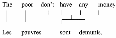
To make this clearer, we consider the example from Brown et al. (Reference Brown, Della Pietra, Della Pietra and Mercer1994: 267), reproduced in Figure 1. We can imagine this example to be one of the ‘documents’ from a parallel corpus, and for the moment we defer discussion of where the term alignments come from and what we do with them.

Fig. 1.

An alignment between English and French.

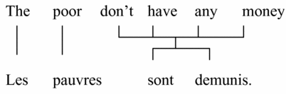
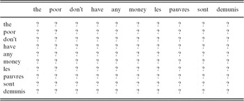
In the traditional LSA-based approach to cross-language IR exemplified in Young (Reference Young1994), this is treated as a bilingual document consisting of ten terms, in English and four in French. Whether or not other documents exist in the corpus, the SVD of the term-by-document matrix X, in which this document would be represented by one column, is equivalent (as mentioned above) to computing the eigenvalues and eigenvectors of XX^T. As the ten terms co-occur in this document (and perhaps others), there will be non-zero entries for each of the 100 pairs in XX^T, as shown in Table 5, in which each entry ‘?’ denotes some non-zero value.

Table 5.

Co-occurrences of English and French terms

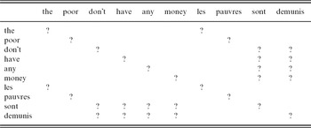
Even though it is not necessarily implied that all ? entries in Table 5 are equal to one another, this data structure fails to encode the term alignments identified by Brown et al. (Reference Brown, Della Pietra, Della Pietra and Mercer1994) and shown in Figure 1. A data structure that would better achieve this is shown in Table 6, a much sparser term–term alignment matrix. As each term aligns with itself, the diagonal of the matrix is filled with non-zero values.

Table 6.

Alignment between English and French terms, in matrix format

Let us consider now how we may supply values for each element (i ₁, i ₂) in either Table 5 or Table 6. As in the cases of term weighting and morphological analysis, we can look to CL for a solution – and the solution again has a basis in IT. The particular subfield of CL which is relevant here is SMT (Brown et al. Reference Brown, deSouza, Mercer, Della Pietra and Lai1992), which, as we have already mentioned, relies upon the alignment of terms using Bayes' theorem and is explicitly informed by communication theory. In vector-space terms, we may restate the procedure for term-alignment from a parallel corpus as follows.

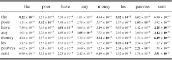
First, for every pair of terms (i ₁, i ₂) that co-occur in the corpus, we compute the mutual information of i ₁ and i ₂. In Section 2.2, we proposed a weighting scheme for the term-by-document matrix which was based on mutual information, but in that case we were dealing with the PMI of a term and document as events or outcomes. Here, by contrast, the mutual information is that of i ₁ and i ₂ as random binary variables. To be explicit, the mutual information I(A; B) of two variables A and B can be stated as follows:

1. (8)

As should be clear by comparing (4) and (8), the relationship of I(A; B) to PMI is that I(A; B) is equal to the expected value of the PMI of all possible outcomes a and b (just as entropy is the expected value of the log-probabilities). An expression that is equivalent to (8) is as follows:

1. (9)

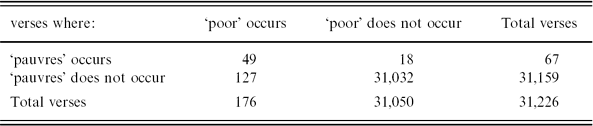
where H(A) and H(B) are the respective entropies of A and B (comparable to term entropy in the log-entropy weighting scheme, but not quite identical because here we treat A and B as binary variables), and H(A, B) is the joint entropy of A and B. To elucidate further how this applies linguistically, let us suppose i ₁ and i ₂ are terms in a corpus. For each document, there are four possibilities: both occur, neither occur, only i ₁ occurs, or only i ₂ occurs. We can represent the distribution of documents according to these four categories in a 2 × 2 matrix. For example, the distribution of ‘poor’ and ‘pauvres’ in the Bible is shown in Table 7 (one row and column are added to show the totals).

Table 7.

Alignment between English and French terms, in matrix format

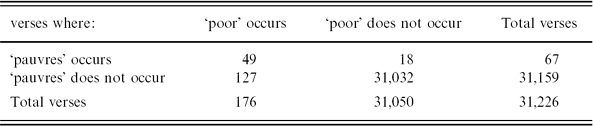
Clearly, mutual information should be maximized when the on-diagonal values are high and the off-diagonal values approach 0. This will generally be true for terms that are truly related to one another, such as ‘poor’ and ‘pauvres’, and not for unrelated pairs, such as ‘poor’ and ‘sont’. In fact, the approximate respective mutual information of these two pairs in the Bible is 1.03 × 10⁻² (which can be confirmed by applying (8) to the data given in Table 7) and 3.92 × 10⁻⁶.

We have already stated that while all entries in Table 5 are non-zero, some are larger than others. With measures of mutual information, we can begin to flesh out this statement more fully by supplying actual values throughout the matrix; this is done in Table 8 (here, the terms ‘don't’ and ‘demunis’ are ignored because they are absent from our parallel corpus, to be described in more detail in Section 4). The result is similar to XX^T, as described above, although the numerical values in each cell may differ from those in XX^T.

Table 8.

Mutual information of English and French terms

The second step when we perform cross-language term alignment in SMT, however, is to pair each term with its most related term in the other language, or to select the pairing that maximizes mutual information and discard those that do not. For each language pair, the terms that maximize mutual information (row-wise) are shown in bold in Table 8. We therefore propose that the term–term matrix should be made sparse by setting all entries for ‘non-aligned’ terms (according to the SMT definition) to zero, which returns us to a situation where the term–term matrix resembles Table 6. This square matrix can then be subjected to Eigenvalue Decomposition (EVD), and the term-by-concept U matrix we obtain will be comparable to that obtained using ‘traditional’ LSA.

For IR based on matrix decomposition, what this boils down to is a choice between using a sparse matrix like in Table 6 or a denser matrix like in Table 5.Footnote ⁵ At least in the case of cross-language IR, the former brings us more into line with SMT, while the latter is essentially akin to the traditional approach to cross-language IR exemplified in Young (Reference Young1994). The former leverages the insight that terms (or, failing that, phrases) can be translated in isolation from one another; the latter assumes that the whole context of a document (or parallel text chunk) is needed for an accurate specification of the terms. To a linguist, the former is intuitively superior, and, as we shall show by an empirical comparison in Section 4, EVD of a matrix like in Table 6 also yields better empirical results than EVD of a matrix like in Table 5.

2.6 Tensor data structures and decompositions

The techniques discussed up to this point remain firmly within the bounds of matrix data structures and decompositions. For the sake of completeness, we now describe some possibilities for using tensor data structures and decompositions, with a focus on cross-language IR.

A general review of different types of tensor decomposition and their applications is given by Kolda and Bader (Reference Kolda and Bader2009). In text analysis, Liu et al. (Reference Liu, Zhang, Yan, Chen, Liu, Bai and Chien2005) have explored the use of Tucker decomposition for tensors, and PARAFAC has been used for conversation detection in e-mail over time using (1), a three-way term-by-author-by-time tensor, and (2), a four-way term-by-sender-by-recipient-by-time tensor (Bader, Berry and Browne Reference Bader, Berry, Browne, Berry and Castellanos2008; Bader, Berry and Langville Reference Bader, Berry, Langville, Srivastava and Sahami2009). A demonstrated virtue of tensor-based approaches to text analysis is that they allow types of relationship to surface that would not be apparent from matrix-based approaches (for example, conversations between senders and recipients and their localization in time, in the case of the four-way analysis above). However, most datasets on which analysis has been conducted do not support quantitative evaluation of multilinear algebraic (tensor) methods compared to linear algebraic methods. Thus, the previous literature has generally shown only a qualitative rather than quantitative benefit to using tensor methods.

An exception to this is Chew et al. (Reference Chew, Bader, Kolda and Abdelali2007), who have shown that PARAFAC2 can outperform SVD in the same cross-language IR task we consider. In this case, PARAFAC2 is a purely algebraic alternative to our proposal informed by SMT: the data is treated as a three-way term-by-document-by-language tensor, which is then factorized by PARAFAC2. Chew et al. (Reference Chew, Bader, Kolda and Abdelali2007) have show that the tensor-based method significantly outperforms standard LSA when log-entropy weighting is used.

Elsewhere, we have evaluated both Tucker and PARAFAC2, and while our results did improve upon those we obtained with SVD, the improvement was nowhere near as large as that we ultimately obtained (and report upon here) with the SMT-based approach described in this section. As we do not currently see how either tensor-based method can be integrated together with the SMT-based approach, our quantitative experimental results have led us to conclude that the SMT-based approach is to be preferred. We take this as interesting circumstantial evidence, although not a final verdict, that while tensor-based techniques can be helpful, it may be better to look to IT for insights that can truly make headway in improving empirical results.

3.1 Basic IR structure

First, let us set out what is unchanged from the traditional approach. We adhere to the concept of the term-by-document matrix containing numerical entries indicating the strength of association between terms and documents. We have also drawn attention to the use of tensors (e.g. term-by-author-by-time) for natural language processing and IR; though this is not a new idea, it has not gained nearly as much traction in the IR community as the more familiar concept of the term-by-document matrix. We accept that within the general framework of matrix computations, documents are treated as unordered ‘bags of words’. Finally, we recognize the usefulness and applicability of linear (SVD and EVD) and multilinear (e.g. PARAFAC, PARAFAC2) algebraic techniques to factorize and reduce matrices and tensors, although again, SVD is by far the most well-known of these techniques in the IR community.

In addition, there are some general principles of IR that we would like to uphold in our enhanced IR model. All of the techniques listed are instances of unsupervised learning; the structure of a corpus is learned directly from the corpus, through the application of statistics-based algorithms. While one could conceive of using a hand-built grammar (such as a phrase-structure grammar) to tokenize terms morphologically and then treating the resulting morphemes as the new terms (for example, to achieve the goals stated in Section 2.3), this would introduce a requirement for a priori information. The disadvantage of this is that the process as a whole immediately loses some ability to generalize (for example, to new corpora or languages). With all our proposed departures from the standard approach to IR, therefore, we take care to adhere to unsupervised and statistics-driven techniques.

3.2 Our revised approach

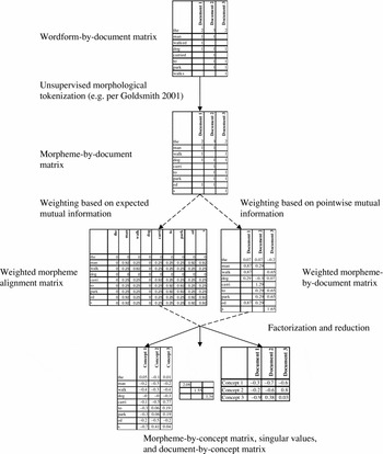
At a high level, we envisage a ‘pipeline’ like that depicted in Figure 2 with various optional elements (denoted by dotted lines). Note that all these elements are contained within the IR ‘training’ phase, meaning that the time required to process data in them is a one-time cost. When the IR framework is deployed on live data, the bulk of the linguistics work is already done; deployment is largely a matter of token-matching and simple arithmetic. In essence, this is why the cost of making the framework linguistically smarter need not be as great as it might first appear.

Fig. 2.

The IR pipeline.

Note that among the optional procedures outlined here, the choice is essentially whether to use a term-by-document matrix, a term-by-term alignment matrix as proposed in Section 2.4, or both (as discussed below). We believe that the use of an alignment matrix is indicated principally for the special case of cross-language IR, in which the training corpus must be a parallel corpus. Even in this case, it is possible to dispense with the alignment matrix and still achieve acceptable results. However, this fails to leverage all available information (in particular, the idea that terms align across language boundaries), and, as shall be shown in Section 4, it is by far preferable to use the alignment matrix when it is known that the base corpus is parallel.

3.3 Combining term-by-term and term-by-document matrices

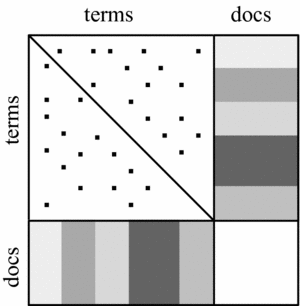
For a document-by-concept matrix to be obtained as output, the term-by-document matrix must be included in the factorization, but so far we have not discussed how to incorporate both term-by-term and term-by-document information in that process. There is another approach to the factorization that can combine the two sources of information and allows the computation of both term-by-concept and document-by-concept matrices, and this is described in Bader and Chew (Reference Bader and Chew2008). We have already mentioned that the SVD of X may be obtained by computing the EVD of XX^T. (More precisely, the left singular vectors of X are equivalent to the eigenvectors of XX^T.) Alternatively and completely equivalently, the SVD of X may be obtained by computing the EVD of the 2 × 2 block matrix

1. (10)

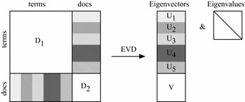
If X is a term-by-document matrix, then the top-left diagonal block of B is a term-by-term matrix and the bottom-right diagonal block is a document-by-document matrix. (We refer to these blocks as D ₁ and D ₂, respectively.) As the standard approach to IR does not take term–term or document–document alignments into consideration, subjecting a term-by-document matrix to SVD (for example, in multilingual IR) is equivalent to the process shown in Figure 3, where the diagonal blocks are empty (or zero).

Fig. 3.

Eigenvalue decomposition in multilingual IR.

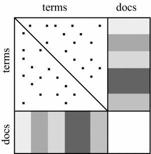
But, as proposed by Hendrickson (Reference Hendrickson2007) and demonstrated by Bader and Chew (Reference Bader and Chew2008), it can be advantageous for the purposes of IR if D ₁ and D ₂ are not empty. In our case, we can place the term–term alignment matrix described in Section 2.4 into its position at D ₁, alongside X and X^T, as shown in Figure 4.Footnote ⁶ The EVD of this square matrix can then be computed to yield both term-by-concept and document-by-concept matrices.

Fig. 4.

Integration of term-alignment information with term-by-document information.

4.1 Use of parallel corpora as a test bed

In much of our work on IR, we have focused on the special case of cross-language IR (CLIR). This is for a variety of reasons. First, CLIR presents interesting challenges. Ideally, we would like to be able to represent terms and documents from multiple languages in a single vector space in a way that is computationally equivalent to breaking down of language barriers. If this can be achieved, then the door is opened to a number of possibilities. For example, the user of a search engine could retrieve documents related to his query, even if the documents are in languages other than that of the query. Likewise, document clustering by topic could be ‘blind’ to the fact that documents are in different languages.

Secondly, CLIR allows our integrated framework to be exercised to the fullest. As already mentioned, we see the greatest benefit in using term-alignment information when a parallel corpus is available.

Third, we would like to be able to claim that the framework is not specific to any language or language group, as far as possible. Deployment on multilingual data allows us to test the extent to which the framework truly is ‘universal’.

Fourth, use of a parallel corpus facilitates certain types of empirical test which are not otherwise possible. For example, we can test the ability of our framework to pair up or cluster parallel documents; the ‘ground truth’ inherent in the corpus' parallelism provides the point of reference for this evaluation, as a translation of a document is surely a relevant response when that document is used as a query. This approach differs from the classical IR approach to evaluation, which involves collecting a set of documents, human-generated queries, and, for each query, a manually validated set of relevant documents (see, for example, Cleverdon Reference Cleverdon1991; Voorhees and Harmaneds Reference Voorhees and Harmaneds2005). It should be noted that our approach to evaluation avoids the subjectivity inherent in manual validation, which is more or less necessitated in monolingual IR (see Swanson Reference Swanson1988).

Finally, at present CLIR is a key research area; this is attributable to a number of factors, including the explosion in on-line resources; the globalization of the world wide webFootnote ⁷; and moves toward political integration in different parts of the world, especially in the European Union.

4.2 Use of the Bible and the Quran as parallel corpora

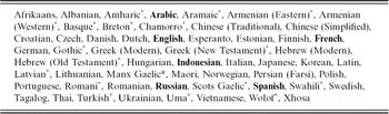
In keeping with our interest in CLIR, we have conducted a large part of our research using the Bible and the Quran as parallel corpora. From various sources, we have gathered texts of the Bible in the fifty-six languages shown in Table 9Footnote ⁸; the six languages in bold (which we refer to as the ‘6 test-language versions’) are those for which we also have texts of the Quran, and the asterisked languages are those for which we do not have a relatively complete translation (meaning that fewer than about 96% of the parallel text chunks are available in the given translation).

Table 9.

Languages available for CLIR validation; bolded entries indicate those we used for our evaluation

For our purposes, an appealing feature of both the Bible and the Quran is that they are, in effect, carefully aligned manually in chunks of approximate sentence length (verses in the case of the Bible, and ayas in the case of the Quran). It should be noted that owing to minor variations in versification between translations, it was necessary for us to perform some initial clean-up as part of the data preparation. After this, we ended up with 31,226 and 6,236 parallel text chunks for the Bible and the Quran, respectively. In both cases, there are also larger natural groupings for the text chunks. In the Bible, the 31,226 verses are grouped into 1,189 chapters, which in turn are grouped into 66 books. In the Quran, the 6,236 ayas are grouped into 114 suras (chapters). To maintain a clean separation between training and test data (the reason we do this is explained further in Section 4.6), we have generally used the verses of the Bible as a training corpus and the 114 suras (chapters) of the Quran as a test corpus, a level of grouping in the test data that allows satisfactory levels of statistical significance to be attained.

An objection which is commonly raised to the use of the Bible and/or the Quran as training and test data is that they may not be very representative of modern language, because in both cases the text is more than a millennium old, and much of the text from the Bible is more than two millennia old. Interestingly Resnik, Broman Olsen and Diab (Reference Resnik, Broman Olsen and Diab1999) have shown that the Bible's vocabulary covers a large percentage of the n most frequent words in the Brown corpus, for various n. Unsurprisingly, the most frequent words in the Brown corpus are best covered, so for example 91% of the top 500 words in the Brown corpus also exist in the NIV translation of the Bible. However, our thesis – that IT can aid IR – does not depend upon overcoming such objections; rather, we view it as a positive benefit that our techniques are developed using a parallel corpus in such a wide variety of languages and versions. In the end, though, the techniques we describe can just as well be applied to ancient text as to modern text, and we are simply applying pattern recognition techniques to strings of symbols. The key point is the comparative evaluation of competing vector-space techniques to a set of data, which is held constant, and we believe that the results we shall present are sufficiently compelling (particularly with regard to statistical significance) as to point to the clear benefit of IT-based techniques for IR. For the avoidance of doubt as to the significance of our results, however, we have repeated our experiments using the French/English portion of the EUROPARL corpus, holding out the data from October–December 2000 as test data (in accordance with standard practice).

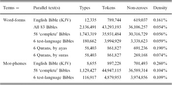
In the Bible, the number of types and tokens of course varies by language, and can also be considered in the aggregate.Footnote ⁹ Some representative statistics are given in Table 10, from which it should be clear that the term-by-document matrices involved are respectably large. Note that the number of non-zeroes in each matrix is always somewhat lower than the number of tokens; the explanation is that in cases where the same type occurs more than once in a particular document, there is more than one token but only one entry in the matrix (an entry greater than 1). Typically for text retrieval, all the matrices are also highly sparse (indicated by the rightmost column in Table 10).

Table 10.

Representative lexical statistics delineating sizes of term-by-document matrices

While it appears possible in CLIR to use incomplete versions, or versions for which only a subset of the parallel chunks exists (Chew and Abdelali Reference Chew and Abdelali2007), our fifty-eight complete parallel versions contained more than enough data for our purposes, and still covered a wide range of heterogeneous languages. Thus, we focused our efforts on the processing of those versions. Restricting the data in that way, we have a slightly smaller wordform-by-document matrix: 1,743,319 types, 35,931,484 tokens, and 30,316,729 non-zeroes.

4.3 Morphological analysis of the parallel corpus

To convert the wordform-by-verse matrix (X) into a morpheme-by-verse matrix, as illustrated in Table 4, we used Linguistica 3.0.0, open-source software for the unsupervised learning of morphology from any given corpus (Goldsmith Reference Goldsmith2001). The text of each parallel version was separately read into that software, the suffix-identification function was used to learn the suffixal morphology of the given language, and then the tokenized version of the corpus was saved. This entire process took us a matter of minutes for each translation in the parallel corpus. We did not use the prefix-identification function, and the suffix-identification function in Linguistica is not iterative, so each wordform was ultimately tokenized into at most two morphemes. Doubtless, therefore, we did not reduce the DL of the corpus to the minimum possible, and further reduction could have been achieved with more work. However, in all cases the DL was lower than before after tokenization.

Another point which should be borne in mind is that Linguistica 3.0.0 cannot be used to learn non-concatenative morphology, such as the root-and-pattern morphology of Hebrew and Arabic. This points to a challenge to our current framework, with respect to its aim for universal applicability to all languages. Notwithstanding this, Hebrew and Arabic do have examples of ‘contiguous’ morphemes alongside the ‘non-contiguous’ roots. Examples from Arabic are the suffix -un and the prefix al-. In our current implementation many Arabic suffixes are correctly identified even if the triliteral roots are not, and this is why the DL for Arabic can be reduced even if the morphological tokenization is imperfect or incomplete. Furthermore, we do not exclude the possibility that there are (undiscovered) methods for morphological tokenization, which can more easily be generalized to different languages. After all, the Semitic root-and-pattern morphology is little different in kind to Indo-European ablaut, exemplified in English ‘sing/sang/sung’; the primary difference is in how productive these similar processes are in the respective language groups.

In any event, after morphological tokenization, each wordform can be associated with one or more morphemes. In algebraic terms, we can represent these associations in a morpheme-by-wordform matrix (which we denote Y). Arriving at the morpheme-by-verse array is then a simple matter: it can be obtained from the matrix multiplication YX. The number of columns is the number of verses (as in X), and the number of rows in YX is the number of morpheme types. Actual representative statistics are given in the latter part of Table 10. As can be seen by inspection of the table, using morphemes rather than wordforms as terms generally reduces the number of rows in X, because the size of the lexicon is a key factor that contributes to a corpus' DL; and it was by reducing the DL that we arrived at a set of morphological tokenizations. It also increases the matrix density, because tokenization can only increase the average number of distinct morphemes per document. As a result, the YX density is greater than that of X, although clearly the matrix is highly sparse in either case.

4.4 PMI weighting of the matrix

The next step is to apply weighting to the morpheme-by-document matrix, for which we use the mutual information weighting described in Section 2.2: for each morpheme–document pair, we replace the raw frequency with the PMI of the morpheme and document. As each morpheme type is associated with a particular parallel version, we can also normalize within YX with respect to the Frobenius norm of each language matrix.Footnote ¹⁰ The linguistic rationale for this step is as follows: As the corpus is parallel, the text in any given language should contain no more or less information than the text in any other language. Therefore, it is appropriate to equalize the contribution to YX of each of the languages. In practice, we have found that this results in a minor empirical improvement, although we shall not present detailed results here, because we feel this would distract from more consequential issues which have more direct linguistic relevance.

To fill in the morpheme–morpheme alignment matrix D ₁, we compute the expected mutual information for each language pair. The result is a large, symmetric square matrix, which is even sparser than the matrices described in Table 10; for example, for the six test-language versions, the matrix is 116,917 × 116,917 with 843,452 non-zeroes (a sparseness of 99.994%). We also normalize D ₁ using the method described in Bader and Chew (Reference Bader and Chew2008).

4.5 Computing the matrix decomposition

Finally, we compute either the SVD of YX, the EVD of the block matrix

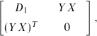
or the EVD of just D ₁, as described above. In all cases, we generally truncate the decomposition to exclude all but the top 300 dimensions. A number of the order of 300 is customary in LSA.Footnote ¹¹ In addition, this corresponds to a point where the values of the diagonal matrix drop off considerably. The result is a morpheme-by-concept matrix U, a set of singular values S, and, so long as the decomposition includes YX, a verse-by-concept matrix V.Footnote ¹² To put it another way, each morpheme (and verse) is represented by a vector in a 300-dimensional ‘concept space’.

4.6 Creation of the test corpus

Just as we form a morpheme-by-verse matrix from the Bible, we can form a morpheme-by-sura matrix from the Quran in a similar way. The procedure for this is as follows. First, a separate wordform-by-sura matrix is formed for each of the six parallel versions of the Quran. This differs from our treatment of the training set: We create separate matrices per language because we want to withhold the ‘parallel’ information to allow for a blind test against what we know to be the ground truth. We can combine these six matrices back into a single matrix (which we denote Q) with 114 × 6, or 684 columns; the number of rows in this matrix is the number of types, which we know from Table 10 is 58,403. Then, to obtain a morpheme-by-sura matrix, we find the product YQ (where Y is the morpheme-by-wordform matrix obtained earlier). Using Y, rather than separately tokenizing the wordforms in Q, or tokenizing the wordforms from X and Q together, allows us to maintain a strict separation of training and test data. However, the consequence is that we have to ignore wordforms that occur in the test set but not in the training set, even if those wordforms contain some morphemes that are present in Y. It would be expected that this would ultimately hurt precision. PMI weighting is then applied to YQ, just as it was applied to YX. Again, we do not create a morpheme-by-morpheme alignment matrix from YQ, because this would require knowledge of the parallel structure of the corpus, which we want to withhold for the purposes of testing. Finally, to project these vectors into the 300-dimension space, we find the product U^TYQ.

An important point with implications for morphology needs to be made here. As matrix multiplication is associative, U^T(YQ) is equivalent to (U^TY)Q, at least if we are dealing with unweighted matrices. With weighting, there is a difference, because in the first case we apply weighting to YQ, then multiply by U^T; in the second, we apply weighting to Q alone. Even so, the results will be approximately the same, no matter whether we think of U^TYQ as morphological tokenization of Q (i.e. YQ) followed by projection into the semantic space, or as projection of wordforms into the semantic space (U^TY) followed by multiplication by Q. As mentioned, an assumption of LSA is that the meaning of a document is in some sense the ‘average’ of the meaning of all its words (Landauer et al. Reference Landauer, Foltz and Laham1998). If this holds true, then it would also be true that the meaning of a wordform is the average of the meaning of all its morphemes. In vector space, finding the meanings of all wordforms in the corpus is tantamount to finding the product U^TY.

4.7 The experiments

Finally, we compute the pairwise cosine similarities between all vectors in U^TYQ to estimate similarities in meaning. For a highly similar pair of documents, the cosine similarity approaches 1, and for dissimilar documents, the cosine similarity will tend to be close to 0. It is also possible to have a negative cosine similarity, which indicates a high negative correlation, although the meaning of this in natural language processing is less clear. Ideally, what we would like to find is that if we rank the results by sura and language, then in order of decreasing cosine similarity (in effect treating each of the 684 vectors as the vector for a query, and retrieving the results in order of relevance), the top six retrieved documents for each sura are the sura itself and its five translations. A numerical measure for this is multilingual precision at six documents or MP6 (Chew et al. Reference Chew, Bader, Kolda and Abdelali2007): the percentage of the top six retrieved results, which are correctly identified as translations, averaged across all queries. Another measure, precision at 1 document (P1), measures the number of times a query vector is most similar to that of its known counterpart in another given language, divided by the total number of queries.

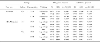
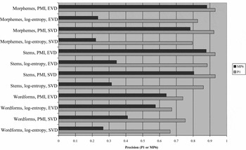
The results of these tests are presented in Table 11 and Figure 5, which show the precision achieved under different settings. It should be evident from Table 11 that our hypothesis – that basing IR more rigorously on concepts from IT should improve the results – is generally borne out. For example, in all cases, use of PMI instead of log-entropy improves precision, and quite significantly in the case of MP6 (in all cases, the increase is highly significant with p < 10⁻¹⁶). We estimate statistical significance here and elsewhere using the chi-squared measure. The most dramatic variations in precision are to be seen for MP6 (which is by definition a stricter measure than P1). In the worst cases, MP6 is scarcely above the baseline of 0.1667.Footnote ¹³

Table 11.

Results with the Bible/Quran and EUROPARL corpora

Notes: (1) Bold type in the settings denotes alternatives that we claim have a stronger basis in IT.

(2) In the first row above, the settings are essentially those of the standard approach to LSA.

(3) In the fifth row, the settings are equivalent to standard LSA with stemming.

(4) The final column averages two measures, which are, strictly speaking, independent of one another. Essentially, this column shows how the results rank if P1 and MP6 are given equal ‘votes’ on the various methods' precision.

(5) SVD is without term alignments and EVD is with term–term alignment and term–document matrices.

Fig. 5.

Charts comparing performance of CLIR framework under various settings.

It is also interesting that to achieve the most meaningful increases in MP6, it is not sufficient to employ any one tactic alone; a systemic approach is needed, just as we have described earlier. For example, under SVD and log-entropy, the use of morphemes rather than wordforms as terms leads to an increase in P1 (from 0.6637 to 0.7953, also significant at p < 10⁻⁷⁰) but a (statistically insignificant) decrease in MP6 (from 0.2264 to 0.2208). The same is true under EVD. Equally, if we hold the settings ‘use wordforms’ and ‘use log-entropy’ constant, the use of EVD rather than SVD results in a considerable increase in MP6 (from 0.2644 to 0.5755) but a statistically insignificant increase for P1 (from 0.6637 to 0.6730). To achieve significant across-the-board increases, PMI must be combined with either the morpheme-based approach or EVD, or preferably both. In our view, this substantiates our argument for the need to follow a coherent approach that is capable of integrating many different ‘modules’.

When morphemes are used as terms, we have the choice of whether or not to include suffixes. If suffixes are excluded, the approach is something like unsupervised stemming. Comparing the eighth and last rows of Table 11, we see that the inclusion of suffixes increases both P1 and MP6 only very slightly: in both cases, though, the increase is statistically insignificant.Footnote ¹⁴ This seems consistent with the hypothesis we advanced in Section 2.3 that suffixes or inflectional endings would be likely to have comparatively low (but not zero) information content, and that their inclusion would therefore not help IR significantly, but would nevertheless be more likely to help than to hurt.

We have observed earlier that with morphemes, there are fewer types (implying a smaller term-by-document matrix to be decomposed) but more tokens, allowing more pattern-matching, but potentially leading to more work at run-time. In our view, any sacrifice of efficiency is worth it in this case; with wordforms as terms, P1 and MP6 are maximized at only 0.7532 and 0.6404, respectively, while with morphemes as terms, maximum values for P1 and MP6 rise to 0.9312 and 0.8818, respectively. These increases are highly significant (p < 0.0001).

We reperformed all of the experiments using the EUROPARL corpus. In both cases, because the dataset was large, we computed a truncated SVD in twenty-five dimensions. The EUROPARL results definitively confirm the superiority of PMI weighting in all cases. They also confirm the utility of MDL-based morphological preprocessing when log-entropy is used, and the value of retaining suffixes when log-entropy and SVD are used. It is less clear from the EUROPARL results that EVD outperforms SVD; there is no statistically significant difference between pairs of results under EVD versus SVD (a difference of around 2–3 percentage points is statistically significant for the EUROPARL tests). One point that should be borne in mind is that the EUROPARL retrieval task is likely easier than the Bible/Quran task for two reasons: first, English and French are closely related, and second, the training and test data for EUROPARL come from the same collection, while the Bible and the Quran were written centuries apart. In view of this, the picture that emerges is that the value of the different strategies that we propose may be greater as the retrieval task gets harder.

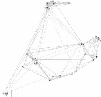
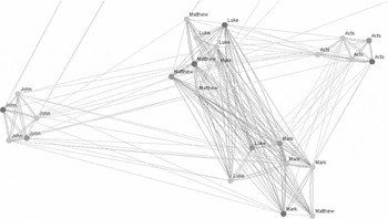
As a demonstration of what can be achieved when the framework achieves high MP6 (around 90 percent), we present in Figures 6 and 7 a partial visualization of how the books of the Bible, color-coded according to language, are represented in the concept vector space.Footnote ¹⁵ Note that the books cluster first to their counterparts in other languages, and then into larger clusters containing related books; this kind of visualization is possible only when MP6 is satisfactorily high. In summary, these techniques have effectively allowed us to factor language out, focusing only on topic, just as we had hoped.

Fig. 6.

Visualization of multilingual Bible books in vector space. Rectangle represents area of details shown in Figure 7.

Fig. 7.

Partial visualization of multilingual Bible books in vector space.