1. Introduction

Surface melt estimates, suitable for describing diurnal variations in melting rates, are desirable but elusive quantities in glacier hydrology. One approach to estimation obtains the energy used in melt as a residual in the surface energy-balance equation (Reference Muller and KeelerMuller and Keeler, 1969, p. 93-95). Successful application of the method to periods of an hour or less requires accurate evaluations of the individual energy-balance terms, principally the surface radiation balance, and the transfer of heat (sensible and latent) from the air to the surface.

The radiation balance can be measured directly, but the transfer of sensible and latent heat fluxes must be calculated from micrometeorological theory using measured profiles of wind speed, temperature, and humidity close to the ice. The theory applies to measurements taken within the turbulent boundary layer of air adjacent to the surface, within which the fluxes are virtually constant with height.

Examples of the energy-balance approach to melt estimation are abundant (Reference DerikxDerikx, 1975; Föhn, 1973; Reference Wendler and IshikawaWendler and Ishikawa, 1973), but few studies have been directed toward the basic question of boundary-layer structure. Some recent studies are useful in this regard (Reference HolmgrenHolmgren, 1971; Reference La CasinèreLa Casinère, 1974, Reference MartinMartin, 1975), though they do not examine the boundary layer per se. Experimental results which illustrate the nature of the turbulent boundary layer over melting ice are presented in this paper.

2. Symbols and units

• L = Monin-Obukhov stability length scale (m)

• Q _H = sensible heat flux (W m⁻²)

• X = Δz/Δ(In z)

• Y = Δy/Δ(In z)

• a = y-intercept of a line

• b = slope of a line

• g = acceleration due to gravity (9.8 m s⁻¹)

• k = von Kármán's constant (0.40)

• p = air pressure (Pa)

• u = wind speed (m s⁻¹)

• u* = friction velocity (m s⁻¹)

• x = horizontal distance (m)

• y = u or θ

• y _* = u _* or θ _*

• z = height (m)

• Zk = katabatic-layer thickness (m)

• z _o = surface roughness length (m)

• Α = Monin-Obukhov constant (dimensionless)

• θ = air temperature (°C)

• θ _a = temperature of undisturbed, advected air (°C)

• θ _b = temperature of advected air cooled by the glacier (°C)

• θ _* = friction temperature (°C)

• p = air density (kg M⁻³)

• τ = momentum flux or shearing stress (Pa)

• ψ = slope angle (degrees)

3. Theory

The general friction-parameter forms of the turbulent transfer equations can be written as

and

Assuming similar transfer mechanisms for both fluxes, a general relationship between gradients and friction parameters is defined by

A method of calculating the fluxes from profile data is obtained if this equation is integrated with respect to height, which yields the familiar logarithmic profile

then rearranged to solve for the friction parameters and combined, in appropriate form with Equations (1). Hence, fluxes can be evaluated from measurements of u, θ and z ₀.

The logarithmic framework assumes that measurements are within the constant-flux layer, and that the lower atmosphere is in a state of neutral equilibrium. Neither of these assumptions is expected to be valid over melting glacier ice because the surface is usually inclined and cold. Hence, in addition to a synoptic-scale pressure-gradient force, local pressure-gradient forces influence the glacier wind (Reference HolmgrenHolmgren, 1971, p. 20-23), and substantial flux divergence can occur close to the surface. Also, the vertical temperature distribution is characterized by inversions which dampen turbulent motion. In this stable state, measured profiles undergo a greater change with height than the logarithmic form predicts.

Following Holmgren (1971, p. 20-23) height-divergence of the momentum flux can be written as

where the terms on the right-hand side are, respectively, the synoptic pressure-gradient force and the local pressure-gradient force (katabatic force). Holmgren (1971, p. 26) showed that the former is smaller in magnitude. Neglecting the synoptic pressure-gradient force, the vertical flux divergence (which is equal to the horizontal flux divergence because of continuity) is equated to the katabatic force:

On the macro scale, the height where the wind speed reaches its free-stream velocity defines τ = 0. In katabatic flow, the momentum flux may reach zero quite close to the surface, where 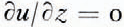(Fig. 3). The height at which 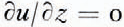will be used here to define the top of the katabatic layer. If this layer is shallow, say a few metres thick, vertical gradients of τ are strong near the surface. According to Equations (1), Q _H must also have a zero value at the top of the katabatic layer. Hence, the flux will diverge in the layer.

Other factors which may contribute to flux divergence are the unsteady nature of katabatic flow, which is evident in short-term accelerations (Reference Lettau and RubinLettau, 1966, p. 7-10), and horizontal temperature and humidity gradients, created by the contrast between the glacier and its surroundings. However, these effects are thought to be relatively small compared to the effect of katabatic layer thickness. In spite of flux divergence, a constant flux layer may be found adjacent to the surface. In this study this will be considered as the boundary layer. Its thickness can be established with profile data if departures from neutral equilibrium are incorporated into the logarithmic framework.

Departures from neutral equilibrium are accommodated by using the log-linear profile (Reference WebbWebb, 1970):

where L is the Monin- Obukhov stability length, defined usually by

and α is an empirically determined constant. The validity of Equation (6a) for stable conditions is well established by experiment, although determinations of α vary. The results of most investigations suggest that the value of α is close to 5 (Reference DyerDyer, 1974, p. 371).

This equation can be used in examining boundary-layer structure following a method outlined by Webb (1970, p. 49-71). If we define the difference in y between two levels above the surface as Δy and divide by Δ(ln z),

where Y = Δy/Δ(In z) and X = Δz/Δ(In z).

With Y and X evaluated from experimental data, Equation (7) takes the form of a linear regression equation, Y = a + bx, where a =Y _*/k and b = (y _*/k)(α/L). Both a and b are positive in turbulent boundary layers in a stable atmosphere. From a, u _* and θ _* are readily calculated and the stability length is obtained from

which is obtained directly from Equations (1) and (6b).

It is proposed to test for boundary-layer occurrence by determining if Y and X are linearly related, with a and b positive. Since the log-linear model is derived with the assumption that fluxes are constant with height, the boundary layer is defined as a zone within which the log-linear model describes the profiles.

4. Site and measurements

A measurement site was established on the tongue of Peyto Glacier (lat. 51° 40' N., long. 116° 33' W.), in the Canadian Rocky Mountains, about 10 km north of Banff, Alberta. The site elevation was 2 300 M. Measurements were taken in August and the first week of September 1971, prior to the end of the ablation season. The ice surface up-wind of the measurement site consisted of elongated ice hummocks, with a local relief of about 0.5 m and z _o = 0.07 mm. The character and relief of the surface appeared to be uniform over a distance of 1 km in the up-wind direction. The surface slope was close to 3°.

Wind-speed and temperature profiles were measured by sensors at heights of 0.25, 0.5, 0.75, 1, 1.5, 2 and 4 m above the surface. On some occasions temperature measurements were also taken at 6 m. Additional wind-speed measurements were made at 2.5, 3, 3.5, 5 and 6 m.

Sensitive cup anemometers (stall speed, 0.1 m s⁻¹) were used to measure the wind speed to ±0.025 m s⁻¹. Ventilated thermopile thermometers measured temperature. Sensor outputs were recorded on a potentiometric recorder (Honeywell Model 194) using a stepping switch. The precision of the temperature measurements was approximately ±o.o4 deg. Data were meaned over 30 min time periods. The range of experimental conditions is shown in the examples of Figure 1. A few matched pairs of the wind and temperature profile are included in order to compare the shapes. Missing data are the result of instrument failure. The profiles show well-defined, smooth variations with height.

Fig. 1.

Selected profiles of (a) wind speed and (b) temperature.

The precision of individual measurements and the magnitudes of Δu and Δθ determined the relative errors in differences between levels. Values for Δu of 0.3 to 0.6 m s⁻¹ are common near the surface, where a precision of 5-10% can be stated for Δu. The error in Δθ is 6 to 14% for typical values of 0.4 to 1°C.

5. Results

Values of u and θ were plotted against In z to see if they conformed to the expected profile form in stable conditions (Fig. 2). The expected form seems to describe the data well within the first metre, but eye-drawn extrapolations of the lower profile form beyond a height of 1 m deviate substantially from the measured values. This suggests a glacier boundary layer with a depth of approximately 1 m. Some wind profiles indicate that Δu approaches 0, and even reverses sign at upper levels (Fig. 2a). Cases where u achieved a maximum value below 6 m were observed infrequently in the data, but all of the profiles showed greater than expected reductions of Δu with increasing height above the surface.

Fig. 2.

Logarithmic plots of (a) wind speed and (h) temperature.

A well-defined example of a wind-speed maximum near the surface is shown in Figure 3. It seems that the zone of highest wind speed is associated with a thermocline. The association is expected. Since u _* approaches 0 as becomes 0, Q _H will also vanish at the top of the katabatic layer (Equation (1b)). Then the thermocline marks the upper limit of the cooling effect of the glacier on adverted air, which becomes thermally separated from the katabatic layer adjacent to the surface. This feature has been observed elsewhere over glaciers (Reference HubleyHubley, 1957; Reference HolmgrenHolmgren, 1971), and it supports the postulated association between katabatic layer thickness and flux divergence.

Application of the Webb (1970, p. 69-71) procedure to the profiles confirms the relative thinness of the glacier boundary layer (Fig. 4). A linear relationship, with positive slope, is found only when measurements taken at 1.5 m or less are used to calculate Y and X in the case of wind speed. The limit appears to be 1 m for temperature. Scatter in the data points is attributed to errors in Δu and ΔT. Hence, the boundary layer is defined to be 1 to 1.5 m thick in this case.

Fig. 3.

Example of katabatic wind and associated thermocline.

Fig. 4.

Example of air layer analysis for 21.00 h, 13 August 1971: (a) from wind-profile data; (b) from temperature-profile data.

Δ adjacent height pairs, the lowest level marked by a numeral (solid within the boundary layer).

? other height pairs (solid within the boundary layer).

_____ joins height pairs with the same lowest level.

…… the best fit of points within the boundary layer.

Inclusion of measurements taken above the boundary layer results in large scatter, but order is achieved by joining all points with the same lower level for Δ(ln z). Points joined in this way follow the line of best fit when calculated from boundary-layer measurements, and parallel one another for measurements above the layer. This result is similar to that obtained by Webb (1970, Fig. 4). The values of Δu/Δ (ln z) show a marked increase at first, due to the thermocline, but decrease as measurements at higher levels are used.

Not all profiles indicated boundary-layer occurrence close to the surface. Plots of Y against X were classified into three groups:

1. boundary-layer cases in which the expected linear relationships were found close to the surface (Fig. 5);

2. cases in which Y decreased with height everywhere above the surface. These were interpreted to be cases where the boundary layer failed to establish itself within the katabatic layer;

3. cases where missing data or large scatter made it impossible to obtain relationships between Y and X: these were discarded.

In all boundary-layer cases the layer thickness appeared to be close to 1 m, with only rare deviations (Fig. 5). Also, boundary-layer depths defined from the wind profile usually coincided with those defined from the temperature profile. The constant α was determined to be 5.4 for the wind profile and 3.6 for the temperature profile from mean values of α = X/L. These results are close to those obtained by other investigators in stable conditions (Dyer,1974, p. 371).

A boundary layer occurs frequently (Table 1) but is not a dominant feature of the air over the ice. There is a tendency for boundary layers to occur more frequently during the day than at night, though it is possible that the difference in sample size affects the result.

The possibility of a diurnal variation in boundary-layer frequency was further examined by analyzing five 24 h periods, thereby equalizing day and night sample sizes (Fig. 6). The result is essentially the same as that obtained from the total sample, but a regular diurnal variation of boundary-layer frequency is not apparent (Fig. 6a).

A higher frequency of boundary-layer occurrence during the day is not strongly supported in results for individual days (Fig. 6b). Some of the records show extended periods of boundary-layer occurrence which are interrupted or abruptly ended by absence. Others appear to be characterized by the total absence of boundary layers. Hence the boundary layer is an ephemeral feature of the air adjacent to the ice, and its occurrence does not follow a simple pattern.

Fig. 5.

Selected friction parameter profiles for (a) wind and (b) temperature.

? boundary layer height in pairs.

? height pairs outside the boundary layer.

- - - - - best fit to points within the boundary layer.

Table I.Summary of boundary layer analysis

Fig. 6.

Frequency of boundary-layer occurrence as a function of time based upon five 24 h periods. In Figure 6a the hatched area (riferred to zero) shows all cases with usable data while the stippled area shows boundary layer cases. In Figure 6b boundary-layer cases are represented by dots and non-boundary layer cases by open circles.

6. Discussion

The reason for the ephemeral nature of the boundary layer may lie in the mechanism which governs the flow. The simplest mechanism would be one in which Equation (5) describes the divergence of momentum flux. The momentum flux at the surface could be defined by integrating Equation (5) with respect to height over the interval Z_k -Z ₀

The surface flux is also obtained by combining Equation (1a) with the log–linear wind profile

Combining Equations (9) and (10)

Hence, wind speed can be estimated from values of θ_a and θ _b Reference HolmgrenHolmgren (1971) suggests using the temperatures above and below the thermocline for θ_a and θ_b respectively. His suggestion is followed here.

In a purely katabatic flow it should be possible to find a linear correlation between u and [(θ _a — θ_b )/θ_a if z ₀, ψ, and z_k are constant. An attempt was made to correlate the wind speed at z = 1 m, the observed top of the boundary layer, with the temperature data. Constraints of the experimental procedure confined θ₀ , to a height of 4 m or less, so 4 m was chosen. θ_b was taken at 1 m, a level which seemed to be well below that of any thermocline, and coincident with that of the wind speed. Thermoclines were classified indirectly through an examination of the wind profile. Assuming that the top of the katabatic layer corresponded to the position of the thermocline, only those cases where z was 4 m or less were considered. The majority of wind-speed maxima were observed close to 3.5 or 4 m in the 96 samples chosen.

Wind speed correlates poorly with (Fig. 7). However, wind speed has a lower limit given by = [In . This was evaluated using α = 5.4, L = ∞ (the neutral case), z ₀ = 0.07 mm, ψ = 3°, and z_k = 4 m. The value of z_k follows from the selection procedure for the data used in the analysis.

Several factors could account for the large scatter of data points in Figure 7, particularly failure to account for stability effects as slope evaluations at other values indicate. Underestimation of the thermocline strength by the difference in temperature between 1 and 4 m is another possible source of error. However, boundary-layer cases make up 80% of the plotted points, a much higher proportion than that for the whole sample. This is instructive because the data were taken during periods where the flow was largely katabatic. Other forces are probably influential as well, notably:

1. forces generated by heating and cooling effects which give rise to valley winds. The winds reverse direction over the course of a day, and cover areas larger than that of the glacier;

2. large-scale pressure-gradient forces. They have been ignored in the initial discussion of the theory, but it is possible that synoptic-scale winds, channelled through mountainous terrain, disturb local wind patterns.

The influence of the glacier on the wind speed is felt whenever the air temperature is above freezing. However, the influence of other forces could be highly variable in time, strongly amplifying or damping the katabatic force on some occasions, hardly affecting it at other times. It is possible that the data selected for Figure 7 were taken at times when outside influences were small. At such times the flow mechanism is relatively simple, and apparently favours boundary-layer development. Alternatively the flow at other times may depend upon a complex mechanism in which several forces interact, reducing the likelihood of boundary-layer occurrence. This view is supported by the constancy of the glacier boundary-layer thickness and the small variation in the thickness of the zone of flux divergence (katabatic layer). They indicate a more-or-less constant ratio of the two thicknesses, which agrees with the general view in boundary-layer work. Consequently, the absence of a wind-speed maximum close to the surface may not indicate a thickening of the katabatic layer, but rather that other forces have become dominant in the control of the glacier wind.

Fig. 7.

Correlation between u and Boundary-layer cases (dots) are distinguished from non-boundary layer cases (open circles). The dotted line is determined from Equation (11), using different L values.

7. Summary and conclusions

This study shows that turbulent-transfer theory may be restricted in its application to heat-flux estimation. The boundary-layer thickness is particularly important in determining the height of measurements. The usual practice of locating meteorological shelters at 1.5 to 2 m above the surface for the purpose of energy-exchange computations, is inappropriate for this site. However, a general criticism of the practice cannot be made because boundary-layer thickness probably depends upon the characteristics of each experimental site. The frequency of boundary-layer occurrence is also important because it determines the long-term effectiveness of the turbulent-transfer approach.

Further study of profile structure at other sites over glaciers is warranted. Particular attention should be directed toward obtaining measurements at many levels within 1 or 2 m of the surface since this appears to be the important region for the application of turbulent-transfer theory.