



1. Introduction
Boundary-layer transition from a laminar to a turbulent regime is a critical driver for the optimal design of high-speed vehicles. Aerothermodynamic loads during hypersonic laminar–turbulent transition can surpass the loads in the laminar regime by an order of magnitude, even overshooting the ones in the fully developed turbulent regime, which can already be several times higher than those in the laminar counterpart. As an example, the turbulent heat-transfer coefficient on a flat plate in free flight at Mach  $6$ and at a Reynolds number of
 $10^7$ is almost one order of magnitude larger than the respective laminar value (van Driest Reference van Driest1956).
One of the factors that are known to affect the boundary-layer transition process at high speed is the presence of localized or distributed roughness on the surface of a vehicle. The perturbations generated by these elements can enhance the growth of incoming disturbances and introduce additional instability mechanisms in the flow field, eventually leading to a premature occurrence of transition. During the re-entry on the final mission of the Space Shuttle Endeavour (STS-134), high-resolution infrared observations were performed by Horvath et al. (Reference Horvath, Zalameda, Wood, Berry, Schwartz, Dantowitz, Spisz and Taylor2012) to obtain quantitative data for the temperature distribution over the windward surface of the orbiter. The results showed that boundary-layer transition started to occur in an asymmetric manner shortly after the nose region. After data analysis, evidence was found that transition was most probably triggered by some form of isolated roughness located in proximity to the starboard rear corner of the nose landing gear door. Related observations were also reported by the Hypersonic Thermodynamic Infrared Measurements (HYTHIRM) team (see Horvath et al. Reference Horvath, Tomek, Berger, Splinter, Zalameda, Krasa, Tack, Schwartz, Gibson and Tietjen2010) during the re-entry of STS-119. In this case, numerical analyses performed by Candler & Campbell (Reference Candler and Campbell2010), employing a turbulence model coupled with a boundary-layer tripping driven by the STS-119 flight measurements, were directly compared against the respective flight thermal imagery and displayed good qualitative agreement. Similarly, wind tunnel experimental investigations have also shown that laminar–turbulent transition can be dominated by roughness effects in a wide range of conditions (see for instance Klebanoff & Tidstrom Reference Klebanoff and Tidstrom1972; Corke, Bar-Sever & Morkovin Reference Corke, Bar-Sever and Morkovin1986; Reda Reference Reda2002; Fujii Reference Fujii2006; Schneider Reference Schneider2008).
The effects of two-dimensional discrete roughness elements on boundary-layer transition were investigated experimentally for subsonic boundary layers by Klebanoff & Tidstrom (Reference Klebanoff and Tidstrom1972), who found that the roughness geometry did not generate any additional instability mechanism in the flow, but rather introduced modifications in the base flow which had a destabilizing influence on already existing disturbances (Tollmien–Schlichting waves in this case). For the case of a Mach  $4.8$ boundary layer, Marxen, Iaccarino & Shaqfeh (Reference Marxen, Iaccarino and Shaqfeh2010) studied the destabilizing effect introduced by a two-dimensional isolated roughness element on the evolution of a small disturbance by means of direct numerical simulation (DNS). The disturbance was generated by blowing and suction at the wall at a location upstream of the roughness element. The roughness was found to accelerate the transition process by introducing a stable mode in the flow which interfered with the upstream disturbance, effectively amplifying it in a given frequency range. Three-dimensional roughness elements with heights comparable to the local boundary-layer thickness usually have a stronger influence on the transition process in supersonic and hypersonic flows. It has been shown both experimentally and numerically that these elements tend to induce counter-rotating streamwise vortices in the wake flow field (see for example Joslin & Grosch Reference Joslin and Grosch1995; Tumin & Reshotko Reference Tumin and Reshotko2005; Iyer & Mahesh Reference Iyer and Mahesh2013; Ruban & Kravtsova Reference Ruban and Kravtsova2013), which lift up low-momentum fluid from the near-wall region and give rise to velocity streaks that are surrounded by regions of high shear and can support the growth of different instabilities (Choudhari et al. Reference Choudhari, Li, Chang, Edwards, Kegerise and King2010; Groskopf, Kloker & Marxen Reference Groskopf, Kloker and Marxen2010a; Kegerise et al. Reference Kegerise, King, Owens, Choudhari, Norris, Li and Chang2012; De Tullio et al. Reference De Tullio, Paredes, Sandham and Theofilis2013; Groskopf & Kloker Reference Groskopf and Kloker2016).
Because of the numerous physical processes that come into play and the wide variety of geometrical configurations that are interesting in practice, roughness-induced transition is still not well understood. As reviewed by Schneider (Reference Schneider2008), current practical methodologies for the prediction of roughness effects on hypersonic boundary-layer transition rely heavily on empirical correlations and extensive wind tunnel testing. As a consequence, there are several sources of uncertainty that need to be taken into account. During the design process, this fact implies the need to account for large safety factors that usually lead to oversized thermal protection systems, with a consequent reduction of payload capacity, which ultimately increases the mission cost. A physical parameter that has been found to play an important role in correlating different roughness-induced transition data is the roughness Reynolds number, defined here as  $Re_h = u_h h / \nu _h$, where
 $u_h$ and
 $\nu _h$ are respectively the streamwise velocity and the kinematic viscosity of the fluid at the location and height (
 $h$) of the roughness element in a smooth boundary layer. As shown in the review of Reda (Reference Reda2002), several existing roughness-dominated transition correlations could be modelled by a critical value of
 $Re_h$. DNS computations by Redford, Sandham & Roberts (Reference Redford, Sandham and Roberts2010) for supersonic flow over a flat plate with an isolated smooth roughness element showed that the critical value of
 $Re_h$ increases proportionally to the parameter
 $M_h T_\infty / T_w$, with
 $M_h$ being the Mach number at the roughness height and location in the undisturbed boundary layer,
 $T_\infty$ the free-stream temperature and
 $T_w$ the wall temperature. Later on, Bernardini et al. (Reference Bernardini, Pirozzoli, Orlandi and Lele2012) proposed a modified roughness Reynolds number definition based on the momentum deficit past the obstacle and an evaluation of the dynamic viscosity at the wall, which allowed them to include the effects of wall temperature and roughness shape in the transition criterion. Another physics-based correlation was proposed by Reshotko & Tumin (Reference Reshotko and Tumin2004) using results from transient growth theory, suggesting that roughness-induced transient growth could be a relevant mechanism for boundary-layer transition in the presence of distributed roughness.
In recent years, a significant number of researchers have focused their efforts on studying the stability characteristics of the wake induced by three-dimensional isolated roughness elements in high-speed flow, using both experimental and numerical techniques (Choudhari et al. Reference Choudhari, Li, Chang, Edwards, Kegerise and King2010; Groskopf et al. Reference Groskopf, Kloker and Marxen2010a; Kegerise et al. Reference Kegerise, King, Owens, Choudhari, Norris, Li and Chang2012; Choudhari et al. Reference Choudhari, Li, Chang, Norris and Edwards2013; De Tullio et al. Reference De Tullio, Paredes, Sandham and Theofilis2013; De Tullio & Sandham Reference De Tullio and Sandham2015; Groskopf & Kloker Reference Groskopf and Kloker2016; Theiss et al. Reference Theiss, Hein, Ali and Radespiel2016; Estruch-Samper et al. Reference Estruch-Samper, Hillier, Vanstone and Ganapathisubramani2017; Di Giovanni & Stemmer Reference Di Giovanni and Stemmer2018). Given the strong inhomogeneity of the wake flow field, numerical analyses based on stability theory generally employ two-dimensional amplitude functions, leading to two-dimensional local linear stability theory (2D-LST), also known as BiGlobal stability theory (Theofilis Reference Theofilis2003), or three-dimensional parabolized stability equations (3D-PSE) (Paredes et al. Reference Paredes, Hanifi, Theofilis and Henningson2015b). These studies have revealed that the roughness wake supports the growth of sinuous and varicose instability modes that develop in the high-shear regions introduced by the counter-rotating vortex pair, and that these disturbances can undergo substantial growth during the linear stages of the transition process. Groskopf et al. (Reference Groskopf, Kloker and Marxen2010a) performed temporal 2D-LST analyses in the wake behind isolated three-dimensional cuboidal roughness elements in a Mach  $4.8$ boundary layer and compared the amplitude functions against DNS data. The results showed the growth of an even (varicose) and an odd (sinuous) instability mode in the wake behind the element, reporting good agreement between the disturbance amplitude shapes and the DNS data. Kegerise et al. (Reference Kegerise, King, Owens, Choudhari, Norris, Li and Chang2012) carried out experimental measurements of the disturbance amplitudes behind a diamond element in a flat plate at Mach
 $3.5$, and compared them against the spatial amplitude signatures obtained by the 2D-LST analyses of Choudhari et al. (Reference Choudhari, Li, Chang, Edwards, Kegerise and King2010) with satisfactory results, reinforcing the validity of the theory for the geometrical configurations considered. Their investigations revealed that, for a roughness Reynolds number of 426, the varicose mode was dominating the transition process, whereas for
 $Re_h = 319$ the sinuous instability was leading.
A sharp-edged cuboid geometry at Mach  $2.5$ was also studied by De Tullio et al. (Reference De Tullio, Paredes, Sandham and Theofilis2013) using DNS as well as spatial 2D-LST and 3D-PSE stability theories. The two-dimensional eigenfunctions obtained from the 2D-LST computations and the growth rates extracted from the 3D-PSE simulations were respectively found to be in very good agreement with the DNS results. In that particular case, the varicose instability was found to drive the transition process until the breakdown to turbulence. The same geometrical configuration at Mach
 $6$ was analysed by De Tullio & Sandham (Reference De Tullio and Sandham2015) by means of DNS. For a roughness element with a height of about half the local boundary-layer thickness, three different modes were found to govern the wake instability, namely, a sinuous mode and two varicose modes. The varicose modes featured higher growth, and their development persisted for a longer distance downstream. Two different mechanisms for the excitation of wake modes were identified. On the one hand, the sinuous instability was found to be excited by the interaction between the external disturbances introduced at the inflow and the recirculation regions induced by the roughness element. On the other hand, the varicose modes were excited by an interaction between the natural boundary-layer modes (Mack's first and second modes) and the roughness wake, leading to the hypothesis that a synchronization mechanism between the boundary-layer modes and the wake modes would lead to the continuous excitation of the wake modes as the boundary-layer modes grow downstream. Paredes et al. (Reference Paredes, De Tullio, Sandham and Theofilis2015a) performed stability computations using the laminar base flows of De Tullio & Sandham (Reference De Tullio and Sandham2015) and also reported good qualitative agreement with the DNS data for the 2D-LST amplitude functions and the 3D-PSE growth rates, respectively. However, a significant discrepancy was found between the 2D-LST and 3D-PSE growth rates.
Van Den Eynde & Sandham (Reference Van Den Eynde and Sandham2016) investigated different roughness geometries for a Mach 6 flow over a flat plate, showing that a smooth ramping of the rear portion of the roughness shape towards the wall could significantly reduce the growth of wake instabilities, due to a weakening of the three-dimensional shear layer surrounding the low-velocity streak. Later on, Groskopf & Kloker (Reference Groskopf and Kloker2016) considered the instabilities induced by skewed roughness elements on top of a flat plate in a Mach 4.8 free stream. In this case, a non-symmetric wake is established behind the elements, featuring a stronger low-speed streak than the symmetric counterpart. Linear stability analyses and DNS results showed that at identical roughness height, larger amplification is achieved for eigenmodes in the oblique configuration. A few works have also focused on roughness elements located on the heat shield of a re-entry capsule. Theiss et al. (Reference Theiss, Hein, Ali and Radespiel2016) performed 2D-LST and 3D-PSE computations in the wake behind different isolated roughness geometries located on the forebody of a generic capsule at Mach 5.9. For all the cases considered, the varicose wake modes were the most amplified in terms of maximum  $N$-factors, with the cylindrical roughness element being the most effective shape. In this case, in contrast to the results of Paredes et al. (Reference Paredes, De Tullio, Sandham and Theofilis2015a), the growth rates of the 2D-LST and the 3D-PSE computations were found to be in good qualitative agreement, with 3D-PSE providing higher growth rates. An important difference with respect to the flat plate studies mentioned before is that, because of the strong bow-shock in front of the capsule, the boundary-layer modes upstream of the roughness elements are highly stabilized, and as a result their interaction with wake modes is not present. Very recently, Di Giovanni & Stemmer (Reference Di Giovanni and Stemmer2018) carried out linear stability and DNS computations for a patch of periodic distributed roughness and DNS computations for a patch of randomly distributed roughness on a blunt-capsule configuration at Mach 5.9. For the periodic case, the growth rates of the symmetric and antisymmetric wake modes were found to be in good agreement between 2D-LST, 3D-PSE and DNS. For the random case, the DNS results revealed a new type of roughness-induced cross-flow instability leading to breakdown to turbulence.
Building upon the findings of previous investigations, the objective of this work is to provide additional understanding of the mechanisms that lead to the excitation of discrete roughness-induced wake modes inside a high-speed boundary layer. For this purpose, 2D-LST computations are performed on the wake behind an isolated roughness element mounted on top of a flat plate inside a cold hypersonic free stream, employing base flows obtained from laminar and steady solutions of the Navier–Stokes equations. The role of different base-flow quantities in the temporal evolution of the amplification rate of the different instabilities developing in the roughness wake is investigated by means of a decomposition of the temporal growth rate into production, dissipation and flux terms. This is achieved by generalizing the temporal growth-rate decomposition derived by Weder, Gloor & Kleiser (Reference Weder, Gloor and Kleiser2015) from the disturbance energy equation developed by Chu (Reference Chu1965) to base flows that depend on two spatial directions. The article is organized as follows. Sections 2 and 3 describe the theoretical framework, formulating the governing equations of the stability problem and describing the temporal growth-rate decomposition employed. Section 4 summarizes the numerical methodology considered to obtain the base-flow solutions and solve the stability problem. The resulting base-flow computations are described in § 5. Finally, § 6 discusses the results of the stability analysis, and concluding remarks are provided in § 7.
2. Governing equations
The governing equations considered in this study are the Navier–Stokes equations without body forces. The non-dimensional primitive flow variables are denoted as density  $\rho$, pressure
 $p$, temperature
 $T$, streamwise velocity
 $u$, wall-normal velocity
 $v$ and spanwise velocity
 $w$. The non-dimensional system of equations can be written in non-conservation form and in a Cartesian reference frame as
 \begin{gather} \dfrac{\textrm{D} \rho}{\textrm{D} t} + \rho \left( \dfrac{\partial u}{\partial x} + \dfrac{\partial v}{\partial y} + \dfrac{\partial w}{\partial z} \right) = 0, \end{gather}
 \begin{gather}\rho \dfrac{\textrm{D} u}{\textrm{D} t} + \dfrac{\partial p}{\partial x} - \dfrac{\partial \tau_{xx}}{\partial x} - \dfrac{\partial \tau_{yx}}{\partial y} - \dfrac{\partial \tau_{zx}}{\partial z} = 0, \end{gather}
 \begin{gather}\rho \dfrac{\textrm{D} v}{\textrm{D} t} + \dfrac{\partial p}{\partial y} - \dfrac{\partial \tau_{xy}}{\partial x} - \dfrac{\partial \tau_{yy}}{\partial y} - \dfrac{\partial \tau_{zy}}{\partial z} = 0, \end{gather}
 \begin{gather}\rho \dfrac{\textrm{D} w}{\textrm{D} t} + \dfrac{\partial p}{\partial z} - \dfrac{\partial \tau_{xz}}{\partial x} - \dfrac{\partial \tau_{yz}}{\partial y} - \dfrac{\partial \tau_{zz}}{\partial z} = 0, \end{gather}
 \begin{gather}\hspace{-8pc}\rho \dfrac{\textrm{D} e}{\textrm{D} t} + p \left( \dfrac{\partial u}{\partial x} + \dfrac{\partial v}{\partial y} + \dfrac{\partial w}{\partial z} \right) + \dfrac{\partial q_x}{\partial x} + \dfrac{\partial q_y}{\partial y} + \dfrac{\partial q_z}{\partial z} - \tau_{xx} \dfrac{\partial u}{\partial x} \nonumber\\
\hspace{3pc}- \tau_{yx} \dfrac{\partial u}{\partial y} - \tau_{zx} \dfrac{\partial u}{\partial z} - \tau_{xy} \dfrac{\partial v}{\partial x} - \tau_{yy} \dfrac{\partial v}{\partial y} - \tau_{zy} \dfrac{\partial v}{\partial z} - \tau_{xz} \dfrac{\partial w}{\partial x} - \tau_{yz} \dfrac{\partial w}{\partial y} - \tau_{zz} \dfrac{\partial w}{\partial z} = 0, \end{gather}
where  $\textrm {D}/\textrm {D}t = \partial /\partial t + u \partial /\partial x + v \partial /\partial y + w \partial /\partial z$ is the substantial derivative operator and
 $e$ is the specific internal energy of the fluid. Under the assumption of a Newtonian fluid, the viscous stresses are given by
 \begin{align} \tau_{xx} &= \frac{1}{Re} \left[ \left( 2\mu + \lambda \right) \dfrac{\partial u}{\partial x} + \lambda \left( \dfrac{\partial v}{\partial y} + \dfrac{\partial w}{\partial z} \right) \right], \quad \tau_{xy} = \tau_{yx} = \frac{\mu}{Re} \left( \dfrac{\partial u}{\partial y} + \dfrac{\partial v}{\partial x} \right), \end{align}
 \begin{align}\tau_{yy} &= \frac{1}{Re} \left[ \left( 2\mu + \lambda \right) \dfrac{\partial v}{\partial y} + \lambda \left( \dfrac{\partial u}{\partial x} + \dfrac{\partial w}{\partial z} \right) \right], \quad \tau_{xz} = \tau_{zx} = \frac{\mu}{Re} \left( \dfrac{\partial u}{\partial z} + \dfrac{\partial w}{\partial x} \right), \end{align}
 \begin{align}\tau_{zz} &= \frac{1}{Re} \left[ \left( 2\mu + \lambda \right) \dfrac{\partial w}{\partial z} + \lambda \left( \dfrac{\partial u}{\partial x} + \dfrac{\partial v}{\partial y} \right) \right], \quad \tau_{yz} = \tau_{zy} = \frac{\mu}{Re} \left( \dfrac{\partial v}{\partial z} + \dfrac{\partial w}{\partial y} \right), \end{align}
where  $\mu$ is the dynamic viscosity of the fluid,
 $\lambda$ is the bulk viscosity coefficient and
 $Re$ denotes the Reynolds number. Additionally, Stokes’ hypothesis is considered, such that
 $\lambda = -2/3\mu$. The conductive heat flux vector is modelled using Fourier's law of heat conduction, whose components are expressed as
 \begin{gather} q_x ={-}\frac{k}{\left( \gamma - 1 \right) Re Pr M^2} \dfrac{\partial T}{\partial x}, \quad q_y ={-}\frac{k}{\left( \gamma - 1 \right) Re Pr M^2} \dfrac{\partial T}{\partial y}, \end{gather}
 \begin{gather}q_z ={-}\frac{k}{\left( \gamma - 1 \right) Re Pr M^2} \dfrac{\partial T}{\partial z}, \end{gather}
where  $k$ is the thermal conductivity of the fluid,
 $\gamma$ is the ratio of specific heats,
 $Pr$ denotes the Prandtl number and
 $M$ denotes the Mach number.
The dimensionless quantities employed are defined as follows:
 \begin{gather} t = \frac{t^d u^d_\infty}{l^d}, \quad x = \frac{x^d}{l^d}, \quad u = \frac{u^d}{u^d_\infty}, \quad v = \frac{v^d}{u^d_\infty}, \quad w = \frac{w^d}{u^d_\infty}, \quad \rho = \frac{\rho^d}{\rho^d_\infty}, \end{gather}
 \begin{gather}p = \frac{p^d}{\rho^d_\infty (u^d_\infty)^2}, \quad T = \frac{T^d}{T^d_\infty}, \quad e = \frac{e^d}{(u^d_\infty)^2}, \quad \mu = \frac{\mu^d}{\mu^d_\infty}, \quad k = \frac{k^d}{k^d_\infty}, \end{gather}
where  $(\cdot )^d$ denotes dimensional quantities and
 $(\cdot )^d_\infty$ the dimensional reference quantities used for non-dimensionalization, which correspond to the free-stream flow conditions. The reference length
 $l^d$ is the Blasius length scale evaluated at the local streamwise coordinate of interest, i.e.
 $l^d = \sqrt {\mu ^d_\infty x^d / (\rho ^d_\infty u^d_\infty )}$. The corresponding dimensionless numbers are defined as
 \begin{equation} Re = \frac{\rho^d_\infty u^d_\infty l^d}{\mu^d_\infty}, \quad Pr = \frac{c^d_p \mu^d_\infty}{k^d_\infty}, \quad M = \frac{u^d_\infty}{a^d_\infty}, \end{equation}
where  $c^d_p$ is the specific heat at constant pressure and
 $a^d_\infty$ is the speed of sound in the free stream.
The fluid is assumed to behave as a calorically perfect gas, which allows the internal energy to be expressed as a linear function of temperature, i.e.  $e = c_v T$, with
 $c_v = 1/[\gamma (\gamma - 1) M^2]$ being the specific heat at constant volume. The speed of sound can be computed as
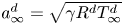 $a^d_\infty = \sqrt {\gamma R^d T^d_\infty }$, where
 $R^d$ is the specific gas constant. Here, the values
 $\gamma = 1.4$ and
 $R^d = 287.18\ \textrm {J}\,(\textrm {kg}\,\textrm {K})^{-1}$ are used. The system of equations is closed with the perfect gas equation of state:
 \begin{equation} p = \frac{\rho T}{\gamma M^2}. \end{equation}
The transport properties  $\mu$ and
 $k$ are assumed to be functions of temperature only, both following Sutherland's law:
 \begin{equation} \mu = T^{3/2} \left( \frac{1 + S^d_\mu/T^d_\infty}{T + S^d_\mu/T^d_\infty} \right), \quad k = T^{3/2} \left( \frac{1 + S^d_k/T^d_\infty}{T + S^d_k/T^d_\infty} \right), \end{equation}
with  $S^d_\mu = 111$ K and
 $S^d_k = 194$ K. The choice of these laws yields a Prandtl number which is not constant through the flow field.
2.1. Linearized perturbation equations
According to linear stability theory, the primitive flow variables  $\boldsymbol {q} = [\rho , u, v, w, T]^\mathrm {T}$ are split into a steady reference state
 $\bar {\boldsymbol {q}}$, also known as base flow, and a small unsteady perturbation field
 $\tilde {\boldsymbol {q}}$:
 \begin{equation} \boldsymbol{q} = \bar{\boldsymbol{q}} + \epsilon \tilde{\boldsymbol{q}} + O(\epsilon^2), \end{equation}
with  $\epsilon \ll 1$. Introducing this splitting into the Navier–Stokes system (2.1) and neglecting nonlinear terms (terms of order
 $O (\epsilon ^2)$) results in the linearized perturbation equations.
In this work, the base flow is assumed to be locally parallel in the streamwise direction, so that  $\bar {\boldsymbol {q}} = \bar {\boldsymbol {q}} (y, z)$ at a given
 $x$ coordinate, and the wall-normal base-flow velocity component (
 $\bar {v}$) is assumed to be zero. The unsteady perturbations are three-dimensional, i.e.
 $\tilde {\boldsymbol {q}} = \tilde {\boldsymbol {q}} (x,y,z,t)$. For these assumptions, the resulting linearized disturbance equations are reported in Appendix A.
2.2. Formulation of the two-dimensional local linear stability problem
To allow the study of the instabilities growing in the wake behind an isolated roughness element, the amplitude of the perturbations is considered to be a function of both the wall-normal and the spanwise directions. This assumption leads to a two-dimensional local linear stability theory (2D-LST), for which the ansatz describing modal perturbations can be written as follows (see for example Theofilis Reference Theofilis2003):
 \begin{equation} \tilde{\boldsymbol{q}} (x,y,z,t) = \hat{\boldsymbol{q}} (y,z) \exp [\mathrm{i} (\alpha x - \omega t)] + \mathrm{c.c.} = 2 \mathrm{Re} \left\{\hat{\boldsymbol{q}} (y,z) \exp [\mathrm{i} (\alpha x - \omega t)] \right\}, \end{equation}
where  $\hat {\boldsymbol {q}}$ is the vector containing the two-dimensional amplitude functions,
 $\alpha$ is the wavenumber along the streamwise direction,
 $\omega$ is the angular frequency and c.c. denotes the complex conjugate. Both
 $\alpha$ and
 $\omega$ can be complex in general. If
 $\alpha$ is assumed to be real and
 $\omega$ is complex, then a temporal stability approach is adopted, in which the imaginary part of
 $\omega$, denoted by
 $\omega _i$, represents the temporal growth rate of the perturbation. On the other hand, if
 $\alpha$ is complex and
 $\omega$ is real, the spatial evolution of the instabilities is considered instead, and the spatial growth rate is given by
 $-\alpha _i$, where
 $\alpha _i$ is the imaginary part of
 $\alpha$.
By introducing (2.9) into the linearized perturbation equations (A1), the 2D-LST equations are obtained. They constitute a partial differential generalized eigenvalue problem which, depending on the approach, can be expressed in matrix form as
 \begin{equation} \boldsymbol{\mathsf{A}}_\omega \hat{\boldsymbol{q}} = \omega \boldsymbol{\mathsf{B}}_\omega \hat{\boldsymbol{q}} \end{equation}
for a temporal analysis, or as
 \begin{equation} \boldsymbol{\mathsf{A}}_\alpha \hat{\boldsymbol{q}} = \alpha \boldsymbol{\mathsf{B}}_\alpha \hat{\boldsymbol{q}} + \alpha^2 \boldsymbol{\mathsf{C}}_\alpha \hat{\boldsymbol{q}} \end{equation}
for a spatial framework. The matrices  $\boldsymbol{\mathsf{A}}$,
 $\boldsymbol{\mathsf{B}}$ and
 $\boldsymbol{\mathsf{C}}$ contain the coefficients of the 2D-LST system of equations that respectively multiply the zeroth, first and second powers of the eigenvalue in each approach. In the spatial case, it should be noted that the problem is nonlinear in the eigenvalue
 $\alpha$. To convert the system into a linear eigenvalue problem, the matrix companion method (Bridges & Morris Reference Bridges and Morris1984) is employed, which introduces four auxiliary variables into the vector of amplitude functions:
 $\alpha \hat {u}$,
 $\alpha \hat {v}$,
 $\alpha \hat {w}$ and
 $\alpha \hat {T}$. This procedure significantly increases the computational cost associated with solving the spatial eigenvalue problem, compared to the temporal one.
3. Disturbance energy evolution equation
An evolution equation for the total energy of a disturbance in a calorically perfect gas was originally derived by Chu (Reference Chu1965) for two-dimensional perturbations developing in base flows that depend only on one spatial dimension. This formulation was later extended by Weder et al. (Reference Weder, Gloor and Kleiser2015) to account also for non-vanishing disturbances at the domain boundaries.
According to Chu (Reference Chu1965), a disturbance energy equation can be obtained by adding all five linearized perturbation equations (A1) together, each of them multiplied by a specific factor, and then integrating the resulting sum over an arbitrary time-dependent domain. The specific multiplicative factors employed by Chu (Reference Chu1965) for each equation are  $\bar {T} \tilde {\rho } / (\gamma M^2 \bar {\rho })$ for the continuity equation (A1a),
 $\tilde {u}$ for the
 $x$-momentum equation (A1b),
 $\tilde {v}$ for the
 $y$-momentum equation (A1c),
 $\tilde {w}$ for the
 $z$-momentum equation (A1d) and
 $\tilde {T}/\bar {T}$ for the energy equation (A1e). This formulation leads to a definition of the disturbance energy which satisfies two fundamental requirements, namely, that the disturbance energy must be a positive definite quantity, and that in the absence of energy sources, the energy of the disturbance must be a monotone non-increasing function of time. However, Chu (Reference Chu1965) points out that it is not obvious whether these two properties are sufficient to uniquely define the energy in a disturbance. A later work by Hanifi, Schmid & Henningson (Reference Hanifi, Schmid and Henningson1996) shows that this formulation of the disturbance energy is actually not unique, and that the choice of the multiplicative factors for each governing equation is arbitrary as long as the resulting disturbance energy quantity satisfies the two requirements previously stated. It is very important to take into account the implications of this fact when defining the disturbance energy in this manner. In particular, it is not appropriate to compare different energy contributions that originate from different equations in the system, since their relative magnitudes depend on the chosen multipliers. For instance, for different choices of the multiplicative factors, the relative magnitudes of terms derived from the momentum equation (kinetic energy) and those derived from the energy equation (internal energy) are different.
In this work, the derivation of Chu (Reference Chu1965) is generalized to three-dimensional perturbations developing in base flows that depend on two spatial directions. Denoting an infinitesimal volume element by  $\textrm {d} \mathcal {V} = \textrm {d} x\,\textrm {d} y\,\textrm {d} z$, belonging to the integration domain
 $\varOmega$, and an infinitesimal surface element by
 $\textrm {d} S$, belonging to the integration boundary
 $\varGamma$, the following (power) equation describing the temporal evolution of the disturbance energy in base flows depending on
 $y$ and
 $z$ can be retrieved:
 \begin{gather} \dfrac{\textrm{d} \tilde{E}}{\textrm{d} t} ={-}\int_\varOmega \bar{\rho} \tilde{u} \tilde{v} \dfrac{\partial \bar{u}}{\partial y}\, \textrm{d} \mathcal{V} - \int_\varOmega \bar{\rho} \tilde{u} \tilde{w} \dfrac{\partial \bar{u}}{\partial z}\, \textrm{d} \mathcal{V} - \int_\varOmega \bar{\rho} \tilde{v}^2 \dfrac{\partial \bar{v}}{\partial y}\, \textrm{d} \mathcal{V} - \int_\varOmega \bar{\rho} \tilde{v} \tilde{w} \dfrac{\partial \bar{v}}{\partial z}\, \textrm{d} \mathcal{V} \end{gather}
 \begin{gather}- \int_\varOmega \bar{\rho} \tilde{w} \tilde{v} \dfrac{\partial \bar{w}}{\partial y}\, \textrm{d} \mathcal{V} - \int_\varOmega \bar{\rho} \tilde{w}^2 \dfrac{\partial \bar{w}}{\partial z}\, \textrm{d} \mathcal{V} - \int_\varOmega \tilde{\rho} \tilde{u} \bar{v} \dfrac{\partial \bar{u}}{\partial y}\, \textrm{d} \mathcal{V} - \int_\varOmega \tilde{\rho} \tilde{u} \bar{w} \dfrac{\partial \bar{u}}{\partial z}\, \textrm{d} \mathcal{V} \end{gather}
 \begin{gather}- \int_\varOmega \tilde{\rho} \tilde{v} \bar{v} \dfrac{\partial \bar{v}}{\partial y}\, \textrm{d} \mathcal{V} - \int_\varOmega \tilde{\rho} \tilde{v} \bar{w} \dfrac{\partial \bar{v}}{\partial z}\, \textrm{d} \mathcal{V} - \int_\varOmega \tilde{\rho} \tilde{w} \bar{v} \dfrac{\partial \bar{w}}{\partial y}\, \textrm{d} \mathcal{V} - \int_\varOmega \tilde{\rho} \tilde{w} \bar{w} \dfrac{\partial \bar{w}}{\partial z}\, \textrm{d} \mathcal{V} \end{gather}
 \begin{gather}- \int_\varOmega \bar{\rho} \tilde{v} \tilde{s} \dfrac{\partial \bar{T}}{\partial y}\, \textrm{d} \mathcal{V} - \int_\varOmega \bar{\rho} \tilde{w} \tilde{s} \dfrac{\partial \bar{T}}{\partial z}\, \textrm{d} \mathcal{V} + \int_\varOmega \tilde{Q} \frac{\tilde{T}}{\bar{T}}\, \textrm{d} \mathcal{V} - \int_\varOmega \frac{\tilde{\rho} \tilde{v}}{\bar{\rho}} \dfrac{\partial \bar{p}}{\partial y}\, \textrm{d} \mathcal{V} - \int_\varOmega \frac{\tilde{\rho} \tilde{w}}{\bar{\rho}} \dfrac{\partial \bar{p}}{\partial z}\, \textrm{d} \mathcal{V} \end{gather}
 \begin{gather}- \int_\varOmega \frac{\tilde{p} \tilde{T}}{\bar{T}} \dfrac{\partial \bar{v}}{\partial y}\, \textrm{d} \mathcal{V} - \int_\varOmega \frac{\tilde{p} \tilde{T}}{\bar{T}} \dfrac{\partial \bar{w}}{\partial z}\, \textrm{d} \mathcal{V} - \int_\varOmega \bar{p} \frac{\tilde{\rho}^2}{\bar{\rho}^2} \dfrac{\partial \bar{v}}{\partial y}\, \textrm{d} \mathcal{V} - \int_\varOmega \bar{p} \frac{\tilde{\rho}^2}{\bar{\rho}^2} \dfrac{\partial \bar{w}}{\partial z}\, \textrm{d} \mathcal{V} \end{gather}
 \begin{gather}-
\frac{1}{\gamma \left( \gamma - 1 \right) M^2} \int_\varOmega
\tilde{\rho} \tilde{T} \frac{\bar{v}}{\bar{T}}
\dfrac{\partial \bar{T}}{\partial y}\, \textrm{d}
\mathcal{V} - \frac{1}{\gamma \left( \gamma - 1 \right)
M^2} \int_\varOmega \tilde{\rho} \tilde{T}
\frac{\bar{w}}{\bar{T}} \dfrac{\partial \bar{T}}{\partial
z}\, \textrm{d} \mathcal{V} \end{gather}
 \begin{gather} - \int_\varOmega \left[
\tilde{\tau}_{xx} \dfrac{\partial \tilde{u}}{\partial x} +
\tilde{\tau}_{yy} \dfrac{\partial \tilde{v}}{\partial y} +
\tilde{\tau}_{zz} \dfrac{\partial \tilde{w}}{\partial z} +
\tilde{\tau}_{xy} \left( \dfrac{\partial
\tilde{u}}{\partial y} + \dfrac{\partial
\tilde{v}}{\partial x} \right) + \tilde{\tau}_{xz} \left(
\dfrac{\partial \tilde{u}}{\partial z} + \dfrac{\partial
\tilde{w}}{\partial x} \right) \right. \\ \left. +
\tilde{\tau}_{yz} \left( \dfrac{\partial
\tilde{v}}{\partial z} + \dfrac{\partial
\tilde{w}}{\partial y} \right) \right]\, \textrm{d}
\mathcal{V} + \int_\varOmega \frac{1}{\bar{T}} \left(
\tilde{q}_x \dfrac{\partial }{\partial x} + \tilde{q}_y
\dfrac{\partial }{\partial y} + \tilde{q}_z \dfrac{\partial
}{\partial z} \right) \tilde{T}\, \textrm{d} \mathcal{V} \end{gather}
 \begin{gather} + \int_\varGamma \left[
\tilde{\tau}_{xx} \tilde{u} n_x + \tilde{\tau}_{yy}
\tilde{v} n_y + \tilde{\tau}_{zz} \tilde{w} n_z +
\tilde{\tau}_{xy} \left( \tilde{u} n_y + \tilde{v} n_x
\right) \right. \\ \left. + \tilde{\tau}_{xz}
\left( \tilde{u} n_z + \tilde{w} n_x \right) +
\tilde{\tau}_{yz} \left( \tilde{v} n_z + \tilde{w} n_y
\right) \right] \,\textrm{d} S \end{gather}
 \begin{gather}- \int_\varGamma \left( \tilde{q}_x n_x + \tilde{q}_y n_y + \tilde{q}_z n_z \right) \frac{\tilde{T}}{\bar{T}} \,\textrm{d} S - \int_\varGamma \tilde{p} \left( \tilde{u} n_x + \tilde{v} n_y + \tilde{w} n_z \right) \,\textrm{d} S \end{gather}
 \begin{gather}+ \frac{1}{Re} \int_\varOmega \dfrac{\partial }{\partial y} \left( \tilde{u} \tilde{T} \dfrac{\textrm{d} \bar{\mu}}{\textrm{d} \bar{T}} \dfrac{\partial \bar{u}}{\partial y} \right)\, \textrm{d} \mathcal{V} + \frac{1}{Re} \int_\varOmega \dfrac{\partial }{\partial z} \left( \tilde{u} \tilde{T} \dfrac{\textrm{d} \bar{\mu}}{\textrm{d} \bar{T}} \dfrac{\partial \bar{u}}{\partial z} \right)\, \textrm{d} \mathcal{V} \end{gather}
 \begin{gather}+ \frac{1}{Re} \int_\varOmega \dfrac{\partial }{\partial x} \left( \tilde{v} \tilde{T} \dfrac{\textrm{d} \bar{\mu}}{\textrm{d} \bar{T}} \dfrac{\partial \bar{u}}{\partial y} \right)\, \textrm{d} \mathcal{V} + \frac{1}{Re} \int_\varOmega \dfrac{\partial }{\partial x} \left( \tilde{w} \tilde{T} \dfrac{\textrm{d} \bar{\mu}}{\textrm{d} \bar{T}} \dfrac{\partial \bar{u}}{\partial z} \right)\, \textrm{d} \mathcal{V} \end{gather}
 \begin{gather}+ \frac{1}{Re} \int_\varOmega \dfrac{\partial }{\partial z} \left( \tilde{v} \tilde{T} \dfrac{\textrm{d} \bar{\mu}}{\textrm{d} \bar{T}} \dfrac{\partial \bar{v}}{\partial z} \right)\, \textrm{d} \mathcal{V} + \frac{1}{Re} \int_\varOmega \dfrac{\partial }{\partial y} \left( \tilde{w} \tilde{T} \dfrac{\textrm{d} \bar{\mu}}{\textrm{d} \bar{T}} \dfrac{\partial \bar{v}}{\partial z} \right)\, \textrm{d} \mathcal{V} \end{gather}
 \begin{gather}+ \frac{1}{Re} \int_\varOmega \dfrac{\partial }{\partial z} \left( \tilde{v} \tilde{T} \dfrac{\textrm{d} \bar{\mu}}{\textrm{d} \bar{T}} \dfrac{\partial \bar{w}}{\partial y} \right)\, \textrm{d} \mathcal{V} + \frac{1}{Re} \int_\varOmega \dfrac{\partial }{\partial y} \left( \tilde{w} \tilde{T} \dfrac{\textrm{d} \bar{\mu}}{\textrm{d} \bar{T}} \dfrac{\partial \bar{w}}{\partial y} \right)\, \textrm{d} \mathcal{V} \end{gather}
 \begin{gather}+ \frac{2}{Re} \int_\varOmega \dfrac{\partial }{\partial y} \left( \tilde{v} \tilde{T} \dfrac{\textrm{d} \bar{\mu}}{\textrm{d} \bar{T}} \dfrac{\partial \bar{v}}{\partial y} \right)\, \textrm{d} \mathcal{V} + \frac{2}{Re} \int_\varOmega \dfrac{\partial }{\partial z} \left( \tilde{w} \tilde{T} \dfrac{\textrm{d} \bar{\mu}}{\textrm{d} \bar{T}} \dfrac{\partial \bar{w}}{\partial z} \right)\, \textrm{d} \mathcal{V} \end{gather}
 \begin{gather}+ \frac{1}{Re} \int_\varOmega \dfrac{\partial }{\partial x} \left( \tilde{u} \tilde{T} \dfrac{\textrm{d} \bar{\lambda}}{\textrm{d} \bar{T}} \dfrac{\partial \bar{v}}{\partial y} \right)\, \textrm{d} \mathcal{V} + \frac{1}{Re} \int_\varOmega \dfrac{\partial }{\partial y} \left( \tilde{v} \tilde{T} \dfrac{\textrm{d} \bar{\lambda}}{\textrm{d} \bar{T}} \dfrac{\partial \bar{v}}{\partial y} \right)\, \textrm{d} \mathcal{V} \end{gather}
 \begin{gather}+ \frac{1}{Re} \int_\varOmega \dfrac{\partial }{\partial z} \left( \tilde{w} \tilde{T} \dfrac{\textrm{d} \bar{\lambda}}{\textrm{d} \bar{T}} \dfrac{\partial \bar{v}}{\partial y} \right)\, \textrm{d} \mathcal{V} + \frac{1}{Re} \int_\varOmega \dfrac{\partial }{\partial x} \left( \tilde{u} \tilde{T} \dfrac{\textrm{d} \bar{\lambda}}{\textrm{d} \bar{T}} \dfrac{\partial \bar{w}}{\partial z} \right)\, \textrm{d} \mathcal{V} \end{gather}
 \begin{gather}+ \frac{1}{Re} \int_\varOmega \dfrac{\partial }{\partial y} \left( \tilde{v} \tilde{T} \dfrac{\textrm{d} \bar{\lambda}}{\textrm{d} \bar{T}} \dfrac{\partial \bar{w}}{\partial z} \right)\, \textrm{d} \mathcal{V} + \frac{1}{Re} \int_\varOmega \dfrac{\partial }{\partial z} \left( \tilde{w} \tilde{T} \dfrac{\textrm{d} \bar{\lambda}}{\textrm{d} \bar{T}} \dfrac{\partial \bar{w}}{\partial z} \right)\, \textrm{d} \mathcal{V} \end{gather}
 \begin{gather}- \frac{1}{2} \int_\varOmega \dfrac{\partial }{\partial x} \left[ \bar{u} \bar{p} \frac{\tilde{\rho}^2}{\bar{\rho}^2} + \frac{\bar{u} \bar{p}}{\gamma - 1} \frac{\tilde{T}^2}{\bar{T}^2} + \bar{u} \bar{\rho} \left( \tilde{u}^2 + \tilde{v}^2 + \tilde{w}^2 \right) \right]\, \textrm{d} \mathcal{V} \end{gather}
 \begin{gather}- \frac{1}{2} \int_\varOmega \left[ \bar{v} \frac{\bar{p}}{\bar{\rho}^2} \dfrac{\partial \tilde{\rho}^2}{\partial y} + \frac{\bar{v} \bar{p}}{(\gamma - 1) \bar{T}^2} \dfrac{\partial \tilde{T}^2}{\partial y} + \bar{v} \bar{\rho} \dfrac{\partial }{\partial y} \left( \tilde{u}^2 + \tilde{v}^2 + \tilde{w}^2 \right) \right]\, \textrm{d} \mathcal{V} \end{gather}
 \begin{gather}- \frac{1}{2} \int_\varOmega \left[ \bar{w} \frac{\bar{p}}{\bar{\rho}^2} \dfrac{\partial \tilde{\rho}^2}{\partial z} + \frac{\bar{w} \bar{p}}{(\gamma - 1) \bar{T}^2} \dfrac{\partial \tilde{T}^2}{\partial z} + \bar{w} \bar{\rho} \dfrac{\partial }{\partial z} \left( \tilde{u}^2 + \tilde{v}^2 + \tilde{w}^2 \right) \right]\, \textrm{d} \mathcal{V}, \end{gather}
where  $\tilde {E}$ is the total disturbance energy, defined as
 \begin{equation} \tilde{E} = \frac{1}{2} \int_\varOmega \left[ \bar{\rho} \left( \tilde{u}^2 + \tilde{v}^2 + \tilde{w}^2 \right) + \frac{\bar{T} \tilde{\rho}^2}{\gamma M^2 \bar{\rho}} + \frac{\bar{\rho} \tilde{T}^2}{\gamma (\gamma - 1) M^2 \bar{T}} \right]\, \textrm{d} \mathcal{V}. \end{equation}
The previous expression (3.2) for the perturbation energy is directly obtained by collecting all the time derivative terms appearing when building (3.1). According to Chu (Reference Chu1965), the first term inside the integral represents the kinetic energy in the disturbance per unit volume, whereas the second and third terms together can be interpreted as the generalized disturbance potential energy per unit volume.
The components of the outward unit vector normal to  $\varGamma$ are denoted by
 $n_x$,
 $n_y$ and
 $n_z$. The quantity
 $\tilde {s}$ is the specific disturbance entropy, which can be expressed as a function of the density and temperature of the perturbation through the following relation:
 \begin{equation} \tilde{s} = \frac{1}{\gamma M^2} \left[ \frac{1}{\gamma - 1} \left( \frac{\tilde{T}}{\bar{T}} \right) - \frac{\tilde{\rho}}{\bar{\rho}} \right]. \end{equation}
Equation (3.3) can be derived from the thermodynamic relationship that quantifies the change in entropy in a calorically perfect gas,  $s - s_{ref} = 1/(\gamma M^2) [1/(\gamma - 1) \ln (T/T_{ref}) + \ln (\rho _{ref} / \rho )]$, together with the assumption of small perturbations, requiring a Taylor expansion of
 $\ln (1 + \tilde {T}/\bar {T})$ and
 $\ln (1 + \tilde {\rho }/\bar {\rho })$ around
 $0$ (also known as the Mercator series).
The disturbance viscous stresses are given by
 \begin{align} \tilde{\tau}_{xx} &= \frac{1}{Re} \left[ \left( 2 \bar{\mu} + \bar{\lambda} \right) \dfrac{\partial \tilde{u}}{\partial x} + \bar{\lambda} \left( \dfrac{\partial \tilde{v}}{\partial y} + \dfrac{\partial \tilde{w}}{\partial z} \right) \right], \quad \tilde{\tau}_{xy} = \frac{\bar{\mu}}{Re} \left( \dfrac{\partial \tilde{u}}{\partial y} + \dfrac{\partial \tilde{v}}{\partial x} \right), \end{align}
 \begin{align}\tilde{\tau}_{yy} &= \frac{1}{Re} \left[ \left( 2 \bar{\mu} + \bar{\lambda} \right) \dfrac{\partial \tilde{v}}{\partial y} + \bar{\lambda} \left( \dfrac{\partial \tilde{u}}{\partial x} + \dfrac{\partial \tilde{w}}{\partial z} \right) \right], \quad \tilde{\tau}_{xz} = \frac{\bar{\mu}}{Re} \left( \dfrac{\partial \tilde{u}}{\partial z} + \dfrac{\partial \tilde{w}}{\partial x} \right), \end{align}
 \begin{align}\tilde{\tau}_{zz} &= \frac{1}{Re} \left[ \left( 2 \bar{\mu} + \bar{\lambda} \right) \dfrac{\partial \tilde{w}}{\partial z} + \bar{\lambda} \left( \dfrac{\partial \tilde{u}}{\partial x} + \dfrac{\partial \tilde{v}}{\partial y} \right) \right], \quad \tilde{\tau}_{yz} = \frac{\bar{\mu}}{Re} \left( \dfrac{\partial \tilde{v}}{\partial z} + \dfrac{\partial \tilde{w}}{\partial y} \right), \end{align}
and the perturbation heat-flux components by
 \begin{equation} \tilde{q}_x ={-}\frac{\bar{k}}{\left( \gamma - 1 \right) Re Pr M^2} \dfrac{\partial \tilde{T}}{\partial x}, \quad \tilde{q}_y ={-}\frac{\bar{k}}{\left( \gamma - 1 \right) Re Pr M^2} \dfrac{\partial \tilde{T}}{\partial y}, \end{equation}
 \begin{equation}\tilde{q}_z ={-}\frac{\bar{k}}{\left( \gamma - 1 \right) Re Pr M^2} \dfrac{\partial \tilde{T}}{\partial z}. \end{equation}
The quantity  $\tilde {Q}$ denotes the specific disturbance heat source, expressed as
 \begin{align}
\tilde{Q} &= \frac{1}{Re} \left( 2 \bar{\mu} -
\dfrac{\textrm{d} \bar{\mu}}{\textrm{d} \bar{T}} \bar{T}
\right) \left[ \dfrac{\partial \bar{u}}{\partial y} \left(
\dfrac{\partial \tilde{u}}{\partial y} + \dfrac{\partial
\tilde{v}}{\partial x} \right) + \dfrac{\partial
\bar{u}}{\partial z} \left( \dfrac{\partial
\tilde{u}}{\partial z} + \dfrac{\partial
\tilde{w}}{\partial x} \right) + 2 \dfrac{\partial
\bar{v}}{\partial y} \dfrac{\partial \tilde{v}}{\partial y}
\right.\nonumber\\ &\quad+ \left. \left( \dfrac{\partial
\bar{v}}{\partial z} + \dfrac{\partial \bar{w}}{\partial y}
\right) \left( \dfrac{\partial \tilde{v}}{\partial z} +
\dfrac{\partial \tilde{w}}{\partial y} \right) + 2
\dfrac{\partial \bar{w}}{\partial z} \dfrac{\partial
\tilde{w}}{\partial z} \right]\nonumber\\ &\quad + \frac{1}{Re}
\left( 2 \bar{\lambda} - \dfrac{\textrm{d}
\bar{\lambda}}{\textrm{d} \bar{T}} \bar{T} \right) \left(
\dfrac{\partial \bar{v}}{\partial y} + \dfrac{\partial
\bar{w}}{\partial z} \right) \left( \dfrac{\partial
\tilde{u}}{\partial x} + \dfrac{\partial
\tilde{v}}{\partial y} + \dfrac{\partial
\tilde{w}}{\partial z} \right)\nonumber\\ &\quad + \frac{1}{\left(
\gamma - 1 \right) Re Pr M^2} \frac{\bar{k}}{\bar{T}}
\left( \dfrac{\partial \bar{T}}{\partial y} \dfrac{\partial
\tilde{T}}{\partial y} + \dfrac{\partial \bar{T}}{\partial
z} \dfrac{\partial \tilde{T}}{\partial z}
\right)\nonumber\\ &\quad + \frac{1}{Re} \tilde{T}
\dfrac{\textrm{d} \bar{\mu}}{\textrm{d} \bar{T}} \left[
\left( \dfrac{\partial \bar{u}}{\partial y} \right)^2 +
\left( \dfrac{\partial \bar{u}}{\partial z} \right)^2 + 2
\left( \dfrac{\partial \bar{v}}{\partial y} \right)^2 +
\left( \dfrac{\partial \bar{v}}{\partial z} \right)^2 +
\left( \dfrac{\partial \bar{w}}{\partial y} \right)^2
\right.\nonumber\\ &\quad + \left. 2 \left( \dfrac{\partial
\bar{w}}{\partial z} \right)^2 + 2 \dfrac{\partial
\bar{v}}{\partial z} \dfrac{\partial \bar{w}}{\partial y}
\right] + \frac{1}{Re} \tilde{T} \dfrac{\textrm{d}
\bar{\lambda}}{\textrm{d} \bar{T}} \left[ \left(
\dfrac{\partial \bar{v}}{\partial y} \right)^2 + \left(
\dfrac{\partial \bar{w}}{\partial z} \right)^2 + 2
\dfrac{\partial \bar{v}}{\partial y} \dfrac{\partial
\bar{w}}{\partial z} \right]\nonumber\\ &\quad + \frac{1}{\left(
\gamma - 1 \right) Re Pr M^2} \left[ \dfrac{\partial
}{\partial y} \left( \tilde{T} \dfrac{\textrm{d}
\bar{k}}{\textrm{d} \bar{T}} \dfrac{\partial
\bar{T}}{\partial y} \right) + \dfrac{\partial }{\partial
z} \left( \tilde{T} \dfrac{\textrm{d} \bar{k}}{\textrm{d}
\bar{T}} \dfrac{\partial \bar{T}}{\partial z} \right)
\right].
\end{align}
A considerable number of intermediate steps are necessary to cast equation (3.1) into its final form. Besides the introduction of the disturbance entropy (3.3), integration by parts in space is applied to the terms that contain second derivatives of the perturbation variables. This procedure introduces the surface terms (3.1z), (3.1aa) and (3.1bb). In addition, unlike Chu (Reference Chu1965) and Weder et al. (Reference Weder, Gloor and Kleiser2015), a zero wall-normal pressure gradient is not assumed, which leads to the presence of the term (3.1p).
3.1. Temporal growth-rate decomposition
The substitution of the perturbation ansatz (2.9) into the disturbance energy (3.1) leads to a decomposition of the temporal growth rate into the different terms that contribute to an increase or decrease of the amplitude of a perturbation, which are directly linked to the production and the dissipation of disturbance energy. To derive this decomposition, a temporal stability framework is employed, such that the disturbances are periodic in the streamwise direction (real streamwise wavenumber  $\alpha = \alpha _r$) but allowed to grow or decay in time (complex angular frequency
 $\omega = \omega _r + \mathrm {i} \omega _i$).
It is worth noting that all the integrands in (3.1) involve products of two disturbance quantities. Following Weder et al. (Reference Weder, Gloor and Kleiser2015), the domain size in the streamwise direction is chosen to be equal to a single wavelength, i.e.  $2 {\rm \pi}/ \alpha _r$, which allows the streamwise integration of disturbance products to be simplified as follows (see also Weder Reference Weder2012):
 \begin{equation} \int_0^{2 {\rm \pi}/ \alpha_r} \tilde{f} \tilde{g}\,\textrm{d} x = \frac{4 {\rm \pi}}{\alpha_r} \exp (2 \omega_i t) \langle \hat{f}, \hat{g} \rangle, \end{equation}
where  $\tilde {f}$ and
 $\tilde {g}$ are two generic disturbance variables, and
 $\langle \hat {f}, \hat {g} \rangle = (\hat {f}^* \hat {g} + \hat {f} \hat {g}^*)/2$, with
 $(\cdot )^*$ denoting the complex conjugate. In addition, because of streamwise periodicity, all the terms with volume integrals of the form
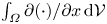 $\int _\varOmega \partial (\cdot ) / \partial x \,\textrm {d} \mathcal {V}$ or with surface integrals of the form
 $\int _\varGamma (\cdot ) n_x \,\textrm {d} S$ become zero. Using (3.7), the disturbance energy can be expressed in terms of the amplitude function of the primitive variables as
 \begin{align}
\tilde{E} &= \frac{4 {\rm \pi}}{\alpha_r} \exp (2 \omega_i t)
\frac{1}{2} \int_{z^-}^{z^+} \int_{y^-}^{y^+} \left[
\bar{\rho} \left( \langle \hat{u}, \hat{u} \rangle +
\langle \hat{v}, \hat{v} \rangle + \langle \hat{w}, \hat{w}
\rangle \right) + \frac{\bar{T}}{\gamma M^2 \bar{\rho}}
\langle \hat{\rho}, \hat{\rho} \rangle \right.\nonumber\\
&\quad + \left. \frac{\bar{\rho}}{\gamma (\gamma - 1) M^2 \bar{T}}
\langle \hat{T}, \hat{T} \rangle \right]\, \textrm{d} y\,
\textrm{d} z = \frac{4 {\rm \pi}}{\alpha_r} \exp (2 \omega_i t)
\hat{E},
\end{align}
where  $\hat {E}$ denotes the perturbation energy amplitude function,
 $z^-$ and
 $z^+$ are respectively the lower and upper limits of the domain along the spanwise direction, and
 $y^-$ and
 $y^+$ are the corresponding limits along the wall-normal direction. Making use of the relation (3.8), the left-hand side of (3.1) becomes
 $\textrm {d} \tilde {E} / \textrm {d}t = 4 {\rm \pi}/ \alpha _r \exp (2 \omega _i t) 2 \omega _i \hat {E}$. Employing (3.7) in all the remaining terms of the disturbance energy equation (3.1) and noting that the factor
 $4 {\rm \pi}/ \alpha _r \exp (2 \omega _i t)$ is common to all terms and cancels out, the following decomposition for the temporal growth rate is obtained:
 \begin{equation} \omega_i = \frac{1}{2 \hat{E}} ( \hat{P} + \hat{D} + \hat{F} ), \end{equation}
where  $\hat {P}$ contains the growth-rate contributions of the energy production terms, which can be either positive or negative depending on the particular conditions;
 $\hat {D}$ encloses the contributions of the energy dissipation terms, which are always negative; and
 $\hat {F}$ comprises the contributions due to the energy fluxes across the domain boundary
 $\varGamma$. Here, the following classification of terms is adopted:
 \begin{gather} \hat{P} = \hat{P}_{RS} + \hat{P}_s + \hat{P}_Q + \hat{P}_{mom} + \hat{P}_{\boldsymbol{\nabla} p} + \hat{P}_{dil} + \hat{P}_{s,T} + \hat{P}_{con}, \end{gather}
 \begin{gather}\hat{D} = \hat{D}_\mu + \hat{D}_k, \end{gather}
 \begin{gather}\hat{F} = \hat{F}_p + \hat{F}_\mu + \hat{F}_k + \hat{F}_{d\mu/dT}, \end{gather}
with
 \begin{align}
\hat{P}_{RS} &={-}\int_{z^-}^{z^+} \int_{y^-}^{y^+}
\bar{\rho} \langle \hat{u}, \hat{v} \rangle \dfrac{\partial
\bar{u}}{\partial y}\, \textrm{d} y\, \textrm{d} z -
\int_{z^-}^{z^+} \int_{y^-}^{y^+} \bar{\rho} \langle
\hat{u}, \hat{w} \rangle \dfrac{\partial \bar{u}}{\partial
z}\, \textrm{d} y\, \textrm{d} z\nonumber\\ &\quad -
\int_{z^-}^{z^+} \int_{y^-}^{y^+} \bar{\rho} \langle
\hat{v}, \hat{v} \rangle \dfrac{\partial \bar{v}}{\partial
y}\, \textrm{d} y\, \textrm{d} z - \int_{z^-}^{z^+}
\int_{y^-}^{y^+} \bar{\rho} \langle \hat{v}, \hat{w}
\rangle \dfrac{\partial \bar{v}}{\partial z}\, \textrm{d}
y\, \textrm{d} z\nonumber\\ &\quad - \int_{z^-}^{z^+}
\int_{y^-}^{y^+} \bar{\rho} \langle \hat{w}, \hat{v}
\rangle \dfrac{\partial \bar{w}}{\partial y}\, \textrm{d}
y\, \textrm{d} z - \int_{z^-}^{z^+} \int_{y^-}^{y^+}
\bar{\rho} \langle \hat{w}, \hat{w} \rangle \dfrac{\partial
\bar{w}}{\partial z}\, \textrm{d} y\, \textrm{d} z,
\end{align}
 \begin{align}
\hat{P}_{s} &={-} \int_{z^-}^{z^+} \int_{y^-}^{y^+}
\bar{\rho} \langle \hat{v}, \hat{s} \rangle \dfrac{\partial
\bar{T}}{\partial y}\, \textrm{d} y\, \textrm{d} z -
\int_{z^-}^{z^+} \int_{y^-}^{y^+} \bar{\rho} \langle
\hat{w}, \hat{s} \rangle \dfrac{\partial \bar{T}}{\partial
z}\, \textrm{d} y\, \textrm{d} z,
\end{align}
 \begin{align} \hat{P}_{Q} &= \int_{z^-}^{z^+} \int_{y^-}^{y^+} \frac{\langle \hat{Q}, \hat{T} \rangle}{\bar{T}}\, \textrm{d} y\, \textrm{d} z, \end{align}
 \begin{align}
\hat{P}_{mom} &={-} \int_{z^-}^{z^+} \int_{y^-}^{y^+}
\langle \hat{\rho}, \hat{u} \rangle \bar{v} \dfrac{\partial
\bar{u}}{\partial y}\, \textrm{d} y\, \textrm{d} z -
\int_{z^-}^{z^+} \int_{y^-}^{y^+} \langle \hat{\rho},
\hat{u} \rangle \bar{w} \dfrac{\partial \bar{u}}{\partial
z}\, \textrm{d} y\, \textrm{d} z\nonumber\\ &\quad -
\int_{z^-}^{z^+} \int_{y^-}^{y^+} \langle \hat{\rho},
\hat{v} \rangle \bar{v} \dfrac{\partial \bar{v}}{\partial
y}\, \textrm{d} y\, \textrm{d} z - \int_{z^-}^{z^+}
\int_{y^-}^{y^+} \langle \hat{\rho}, \hat{v} \rangle
\bar{w} \dfrac{\partial \bar{v}}{\partial z}\, \textrm{d}
y\, \textrm{d} z\nonumber\\ &\quad - \int_{z^-}^{z^+}
\int_{y^-}^{y^+} \langle \hat{\rho}, \hat{w} \rangle
\bar{v} \dfrac{\partial \bar{w}}{\partial y}\, \textrm{d}
y\, \textrm{d} z - \int_{z^-}^{z^+} \int_{y^-}^{y^+}
\langle \hat{\rho}, \hat{w} \rangle \bar{w} \dfrac{\partial
\bar{w}}{\partial z}\, \textrm{d} y\, \textrm{d} z,
\end{align}
 \begin{align} \hat{P}_{\boldsymbol{\nabla} p} &={-} \int_{z^-}^{z^+} \int_{y^-}^{y^+} \frac{\langle \hat{\rho}, \hat{v} \rangle}{\bar{\rho}} \dfrac{\partial \bar{p}}{\partial y}\, \textrm{d} y\, \textrm{d} z - \int_{z^-}^{z^+} \int_{y^-}^{y^+} \frac{\langle \hat{\rho}, \hat{w} \rangle}{\bar{\rho}} \dfrac{\partial \bar{p}}{\partial z}\, \textrm{d} y\, \textrm{d} z, \end{align}
 \begin{align}
\hat{P}_{dil} &={-} \int_{z^-}^{z^+} \int_{y^-}^{y^+}
\frac{\langle \hat{p}, \hat{T} \rangle}{\bar{T}}
\dfrac{\partial \bar{v}}{\partial y}\, \textrm{d} y\,
\textrm{d} z - \int_{z^-}^{z^+} \int_{y^-}^{y^+}
\frac{\langle \hat{p}, \hat{T} \rangle}{\bar{T}}
\dfrac{\partial \bar{w}}{\partial z}\, \textrm{d} y\,
\textrm{d} z\nonumber\\ &\quad - \int_{z^-}^{z^+} \int_{y^-}^{y^+}
\frac{\langle \hat{\rho}, \hat{\rho} \rangle}{\bar{\rho}^2}
\bar{p} \dfrac{\partial \bar{v}}{\partial y}\, \textrm{d}
y\, \textrm{d} z - \int_{z^-}^{z^+} \int_{y^-}^{y^+}
\frac{\langle \hat{\rho}, \hat{\rho} \rangle}{\bar{\rho}^2}
\bar{p} \dfrac{\partial \bar{w}}{\partial z}\, \textrm{d}
y\, \textrm{d} z,
\end{align}
 \begin{align}
\hat{P}_{s,T} &={-} \frac{1}{\gamma \left( \gamma - 1
\right) M^2} \int_{z^-}^{z^+} \int_{y^-}^{y^+}
\frac{\langle \hat{\rho}, \hat{T} \rangle}{\bar{T}} \bar{v}
\dfrac{\partial \bar{T}}{\partial y}\, \textrm{d} y\,
\textrm{d} z\nonumber\\ &\quad - \frac{1}{\gamma \left( \gamma - 1
\right) M^2} \int_{z^-}^{z^+} \int_{y^-}^{y^+}
\frac{\langle \hat{\rho}, \hat{T} \rangle}{\bar{T}} \bar{w}
\dfrac{\partial \bar{T}}{\partial z}\, \textrm{d} y\,
\textrm{d} z,
\end{align}
 \begin{align} \hat{P}_{con} &={-} \int_{z^-}^{z^+} \int_{y^-}^{y^+} \left[ \frac{\bar{v} \bar{p}}{\bar{\rho}^2} \langle \hat{\rho}, \partial \hat{\rho} / \partial y \rangle + \frac{\bar{v} \bar{p}}{(\gamma - 1) \bar{T}^2} \langle \hat{T}, \partial \hat{T} / \partial y \rangle \right. \nonumber\\ &\quad \left. +\, \bar{v} \bar{\rho} \left( \langle \hat{u}, \partial \hat{u} / \partial y \rangle + \langle \hat{v}, \partial \hat{v} / \partial y \rangle + \langle \hat{w}, \partial \hat{w} / \partial y \rangle \right) \vphantom{\frac{\bar{v} \bar{p}}{\bar{\rho}^2}}\right]\, \textrm{d} y\, \textrm{d} z\nonumber\\ &\quad - \int_{z^-}^{z^+} \int_{y^-}^{y^+} \left[ \frac{\bar{w} \bar{p}}{\bar{\rho}^2} \langle \hat{\rho}, \partial \hat{\rho} / \partial z \rangle + \frac{\bar{w} \bar{p}}{(\gamma - 1) \bar{T}^2} \langle \hat{T}, \partial \hat{T} / \partial z \rangle \right. \nonumber\\ &\quad \left. +\, \bar{w} \bar{\rho} \left( \langle \hat{u}, \partial \hat{u} / \partial z \rangle + \langle \hat{v}, \partial \hat{v} / \partial z \rangle + \langle \hat{w}, \partial \hat{w} / \partial z \rangle \right) \vphantom{\frac{\bar{v} \bar{p}}{\bar{\rho}^2}}\right]\, \textrm{d} y\, \textrm{d} z, \end{align}
 \begin{align} \hat{D}_{\mu} &={-} \int_{z^-}^{z^+} \int_{y^-}^{y^+} \left( \langle \hat{\tau}_{xx}, \mathrm{i} \alpha \hat{u} \rangle + \langle \hat{\tau}_{yy}, \partial \hat{v} / \partial y \rangle + \langle \hat{\tau}_{zz}, \partial \hat{w} / \partial z \rangle + \langle \hat{\tau}_{xy}, \partial \hat{u} / \partial y \rangle \right.\nonumber\\ &\quad \left. +\, \langle \hat{\tau}_{xy}, \mathrm{i} \alpha \hat{v} \rangle + \langle \hat{\tau}_{xz}, \partial \hat{u} / \partial z \rangle + \langle \hat{\tau}_{xz}, \mathrm{i} \alpha \hat{w} \rangle + \langle \hat{\tau}_{yz}, \partial \hat{v} / \partial z \rangle \right.\nonumber\\ &\quad \left. +\, \langle \hat{\tau}_{yz}, \partial \hat{w} / \partial y \rangle \right)\, \textrm{d} y\, \textrm{d} z, \end{align}
 \begin{align} \hat{D}_{k} &= \int_{z^-}^{z^+} \int_{y^-}^{y^+} \frac{\langle \hat{q}_x, \mathrm{i} \alpha \hat{T} \rangle + \langle \hat{q}_y, \partial \hat{T} / \partial y \rangle + \langle \hat{q}_z, \partial \hat{T} / \partial z \rangle}{\bar{T}}\, \textrm{d} y\, \textrm{d} z, \end{align}
 \begin{align} \hat{F}_{p} &={-}\int_{z^-}^{z^+} \left. \langle \hat{p}, \hat{v} \rangle \right|_{y^-}^{y^+} \,\textrm{d} z -\int_{y^-}^{y^+} \left. \langle \hat{p}, \hat{w} \rangle \right|_{z^-}^{z^+}\, \textrm{d} y, \end{align}
 \begin{align} \hat{F}_{\mu} &= \int_{z^-}^{z^+} \left. \langle \hat{\tau}_{yy}, \hat{v} \rangle \right|_{y^-}^{y^+} \,\textrm{d} z + \int_{y^-}^{y^+} \left. \langle \hat{\tau}_{zz}, \hat{w} \rangle \right|_{z^-}^{z^+}\, \textrm{d} y + \int_{z^-}^{z^+} \left. \langle \hat{\tau}_{xy}, \hat{u} \rangle \right|_{y^-}^{y^+} \,\textrm{d} z\nonumber\\ &\quad +\, \int_{y^-}^{y^+} \left. \langle \hat{\tau}_{xz}, \hat{u} \rangle \right|_{z^-}^{z^+}\, \textrm{d} y + \int_{z^-}^{z^+} \left. \langle \hat{\tau}_{yz}, \hat{w} \rangle \right|_{y^-}^{y^+} \,\textrm{d} z + \int_{y^-}^{y^+} \left. \langle \hat{\tau}_{yz}, \hat{v} \rangle \right|_{z^-}^{z^+}\, \textrm{d} y, \end{align}
 \begin{align} \hat{F}_{k} &={-}\int_{z^-}^{z^+} \left. \frac{\langle \hat{q}_y, \hat{T} \rangle}{\bar{T}} \right|_{y^-}^{y^+} \,\textrm{d} z -\int_{y^-}^{y^+} \left. \frac{\langle \hat{q}_z, \hat{T} \rangle}{\bar{T}} \right|_{z^-}^{z^+}\, \textrm{d} y, \end{align}
 \begin{align} \hat{F}_{d\mu/dT} &= \frac{1}{Re} \int_{z^-}^{z^+} \left. \langle \hat{u}, \hat{T} \rangle \dfrac{\textrm{d} \bar{\mu}}{\textrm{d} \bar{T}} \dfrac{\partial \bar{u}}{\partial y} \right|_{y^-}^{y^+} \,\textrm{d} z + \frac{1}{Re} \int_{y^-}^{y^+} \left. \langle \hat{u}, \hat{T} \rangle \dfrac{\textrm{d} \bar{\mu}}{\textrm{d} \bar{T}} \dfrac{\partial \bar{u}}{\partial z} \right|_{z^-}^{z^+}\, \textrm{d} y\nonumber\\ &\quad + \frac{1}{Re} \int_{y^-}^{y^+} \left. \langle \hat{v}, \hat{T} \rangle \dfrac{\textrm{d} \bar{\mu}}{\textrm{d} \bar{T}} \dfrac{\partial \bar{v}}{\partial z} \right|_{z^-}^{z^+} \, \textrm{d} y + \frac{1}{Re} \int_{z^-}^{z^+} \left. \langle \hat{w}, \hat{T} \rangle \dfrac{\textrm{d} \bar{\mu}}{\textrm{d} \bar{T}} \dfrac{\partial \bar{v}}{\partial z} \right|_{y^-}^{y^+} \,\textrm{d} z\nonumber\\ &\quad + \frac{1}{Re} \int_{y^-}^{y^+} \left. \langle \hat{v}, \hat{T} \rangle \dfrac{\textrm{d} \bar{\mu}}{\textrm{d} \bar{T}} \dfrac{\partial \bar{w}}{\partial y} \right|_{z^-}^{z^+}\, \textrm{d} y + \frac{1}{Re} \int_{z^-}^{z^+} \left. \langle \hat{w}, \hat{T} \rangle \dfrac{\textrm{d} \bar{\mu}}{\textrm{d} \bar{T}} \dfrac{\partial \bar{w}}{\partial y} \right|_{y^-}^{y^+} \,\textrm{d} z\nonumber\\ &\quad + \frac{2}{Re} \int_{z^-}^{z^+} \left. \langle \hat{v}, \hat{T} \rangle \dfrac{\textrm{d} \bar{\mu}}{\textrm{d} \bar{T}} \dfrac{\partial \bar{v}}{\partial y} \right|_{y^-}^{y^+} \,\textrm{d} z + \frac{2}{Re} \int_{y^-}^{y^+} \left. \langle \hat{w}, \hat{T} \rangle \dfrac{\textrm{d} \bar{\mu}}{\textrm{d} \bar{T}} \dfrac{\partial \bar{w}}{\partial z} \right|_{z^-}^{z^+}\, \textrm{d} y\nonumber\\ &\quad + \frac{1}{Re} \int_{z^-}^{z^+} \left. \langle \hat{v}, \hat{T} \rangle \dfrac{\textrm{d} \bar{\lambda}}{\textrm{d} \bar{T}} \dfrac{\partial \bar{v}}{\partial y} \right|_{y^-}^{y^+} \,\textrm{d} z + \frac{1}{Re} \int_{y^-}^{y^+} \left. \langle \hat{w}, \hat{T} \rangle \dfrac{\textrm{d} \bar{\lambda}}{\textrm{d} \bar{T}} \dfrac{\partial \bar{v}}{\partial y} \right|_{z^-}^{z^+}\, \textrm{d} y\nonumber\\ &\quad + \frac{1}{Re} \int_{z^-}^{z^+} \left. \langle \hat{v}, \hat{T} \rangle \dfrac{\textrm{d} \bar{\lambda}}{\textrm{d} \bar{T}} \dfrac{\partial \bar{w}}{\partial z} \right|_{y^-}^{y^+} \,\textrm{d} z + \frac{1}{Re} \int_{y^-}^{y^+} \left. \langle \hat{w}, \hat{T} \rangle \dfrac{\textrm{d} \bar{\lambda}}{\textrm{d} \bar{T}} \dfrac{\partial \bar{w}}{\partial z} \right|_{z^-}^{z^+}\, \textrm{d} y. \end{align}
The production term  $\hat {P}_{RS}$ represents the work done by the disturbance Reynolds stresses against the velocity shear layers present in the base flow. The term
 $\hat {P}_{s}$ describes the energy produced due to the transport of entropy spottiness across the base-flow temperature shear layers. The next term,
 $\hat {P}_{Q}$, refers to the production of disturbance energy due to the heat source
 $\hat {Q}$, which is generated by transport phenomena, including the variation of the transport properties with temperature. The contribution denoted by
 $\hat {P}_{mom}$ comprises the energy produced as a result of the convection of disturbance momentum across the base-flow velocity shear layers. The presence of a non-negligible pressure gradient in the base flow brings an additional energy production term, labelled as
 $\hat {P}_{\boldsymbol {\nabla } p}$, which can be interpreted as a form of pressure work. Another source of energy production arises from the interaction between pressure and the divergence of the velocity field, which adopts the shape of a pressure dilatation term,
 $\hat {P}_{dil}$. The term
 $\hat {P}_{s,T}$ results from the material derivative of the internal energy fluctuation. The last contribution to the disturbance energy production is comprised inside the term
 $\hat {P}_{con}$, which represents the remaining part of the convective derivative of the total disturbance energy. The dissipation of perturbation energy due to friction and thermal conduction is contained in the dissipation terms
 $\hat {D}_{\mu }$ and
 $\hat {D}_k$, respectively. With regard to the disturbance energy flux, the term
 $\hat {F}_p$ describes the rate of work done on the domain due to the disturbance pressure force. The terms
 $\hat {F}_\mu$ and
 $\hat {F}_k$ respectively embody the net flux of mechanical and thermal energy convected across the domain boundary owing to friction and thermal conduction. Finally, the disturbance energy flux contribution given by
 $\hat {F}_{d \mu / dT}$ appears as a result of the dependence of viscosity on temperature.
In the following sections, the superscript  $d$ employed to denote dimensional quantities is dropped for convenience. Values of quantities presented in dimensional form are unequivocally identified by the accompanying SI units.
4. Numerical methodology
4.1. Details of the base-flow simulations
Two different roughness geometries are considered in this work, which are depicted in figure 1. The first geometry is a sharp-edged cuboidal element with a square planform shape. The second one consists in a three-dimensional sharp-edged ramp geometry, which is inspired by popular passive flow control devices employed to promote boundary layer transition (see for instance Stouffer et al. Reference Stouffer, Baker, Capriotti and Northam1993).
Roughness geometries and computational domain (dashed line). Not to scale.

The geometrical configuration of the computational setup under consideration is also represented in figure 1. A roughness element is mounted on top of a flat plate at a given distance behind the leading edge and centred along the spanwise direction at the streamwise symmetry plane ( $z = 0$). The leading edge of the flat plate is assumed to be infinitely sharp. The computational domain is located inside the shock layer established between the surface and the weak shock wave induced at the flat plate leading edge. This approach reduces the computational effort necessary to obtain the base-flow solution, and has already been employed in similar studies in the literature (see for example De Tullio et al. Reference De Tullio, Paredes, Sandham and Theofilis2013; Di Giovanni & Stemmer Reference Di Giovanni and Stemmer2018). The top boundary has an angle to prevent roughness-induced compression waves and weak shock waves from impinging on it, thus avoiding potential reflections back into the boundary layer. In addition, the spanwise symmetry of the geometrical configuration is exploited by considering only half of the roughness element.
The dimensions of the computational domain are the same for both roughness geometries and are summarized in table 1, which lists the streamwise coordinate and height of the inlet ( $x_{in}, y_{in}$) and outlet (
 $x_{out}, y_{out}$) planes of the domain, as well as the spanwise domain size (
 $z_\infty$), which is constant. Both roughness elements have a height of
 $h = 0.4\ \textrm {mm}$, and their leading edge is located at a streamwise distance of
 $x_h = 60\ \textrm {mm}$ from the flat plate leading edge. Their length is determined according to the ramp angle
 $\theta$ as
 $d = h/ \tan (\theta )$, with
 $\theta = 10^{\circ }$. The roughness Reynolds number for this configuration is
 $Re_h = u_h h / \nu _h = 330$, where
 $u_h$ and
 $\nu _h$ are respectively the streamwise velocity and kinematic viscosity of the flow at a height equal to
 $h$ and at a streamwise location of
 $x_h$ in a self-similar boundary-layer profile. The corresponding ratio of roughness height to the local boundary-layer thickness is
 $h/\delta _{99} = 0.59$, where
 $\delta _{99}$ is estimated by applying the total enthalpy criterion (
 $h_0/h_{0,\infty } = 0.995$) in a self-similar boundary-layer profile at
 $x_h$. The Reynolds number based on the displacement thickness of the boundary layer at the domain inflow is
 $Re_{\delta _1} = 14\,847$.
Dimensions of the computational domain. The origin is located at the flat plate leading edge.

The free-stream values considered for the numerical solution are summarized in table 2. They correspond to the high-Reynolds test conditions of the von Karman Institute H3 hypersonic wind tunnel (Tirtey Reference Tirtey2009). Because of the low free-stream static temperature (total temperature  $T_0 = 500\ \textrm {K}$), no significant excitation of the vibrational molecular energy mode is expected in the flow, and therefore the assumption of a calorically perfect gas is a good approximation. The flat plate wall is assumed to be isothermal with a wall temperature of
 $T_w = 300\ \textrm {K}$. This value corresponds to a cold wall condition, since the adiabatic wall temperature for this flow is estimated to be
 $T_{ad} \approx 430\ \textrm {K}$.
Free-stream conditions used in the base-flow computations.

The numerical solution of the base flow is steady and laminar, and is carried out using the CFD package CFD++® (Chakravarthy et al. Reference Chakravarthy, Peroomian, Goldberg and Palaniswamy1998). The spatial discretization is based on a second-order upwind finite volume scheme that features a limited total variation diminishing flux interpolation together with the Harten–Lax–van Leer–Contact (HLLC) Riemann solver to minimize numerical oscillations in the vicinity of large flow gradients. For time integration, a point-implicit scheme (backward Euler) with multi-grid acceleration and residual smoothing is employed to enhance convergence to the steady state.
With respect to the base-flow boundary conditions, the primitive flow variables are prescribed at the inlet boundary and the top boundary of the domain, using values obtained from a self-similar boundary layer computation. At the centre ( $z = 0$) and at the far-field (
 $z = z_\infty$) streamwise planes, symmetry conditions are specified. At the wall, a no-slip isothermal condition is enforced. Finally, a supersonic outflow boundary condition is specified at the outlet boundary, in which all the primitive flow variables are extrapolated from the interior of the domain.
The computational grids used to obtain the base-flow solutions are block-structured and consist of hexahedral cells. The reference grid resolution employed for each case in every direction is summarized in table 3, resulting in a total of 65 million cells for the cuboid element and 76 million cells for the ramp geometry. A coarser grid resolution used for testing grid convergence is also reported, which corresponds to a reduction of 1/4 in the number of points along each direction. As shown in figure 2, good agreement is achieved between the results obtained for the two grid resolutions.
Convergence of results with respect to the base-flow grid resolution: temperature profiles at  $x = 0.1\ \textrm {m}$ and at the roughness symmetry plane (
 $z = 0$) for
 $(a)$ the cuboid and
 $(b)$ the ramp roughness geometries;
 $(c)$ temporal growth rate as a function of the streamwise direction for a sinuous wake instability of wavelength
 $\lambda _x = 0.325\ \textrm {cm}$ (cuboid) and
 $\lambda _x = 0.86\ \textrm {cm}$ (ramp); shape of the recirculation bubbles induced by
 $(d)$ the cuboid and
 $(e)$ the ramp element at the roughness symmetry plane, represented as isolines of
 $\bar {u} = 0$.

Grid resolution employed for the base-flow computations. The quantities  $N_x$,
 $N_y$ and
 $N_z$ denote the number of grid points along each spatial direction.

4.2. Discretization and solution of the eigenvalue problem
The numerical solution of the stability problem is performed using the von Karman Institute Extensible Stability & Transition Analysis (VESTA) toolkit, originally developed by Pinna (Reference Pinna2013). The terms that constitute the matrices of the stability equations are automatically derived and implemented with a module based on the computer algebra system Maxima. The resulting two-dimensional partial differential eigenvalue problem is assembled and discretized in both spatial directions by means of the high-order finite difference scheme with uniform error developed by Hermanns & Hernández (Reference Hermanns and Hernández2008). Similarly to the Chebyshev collocation method, this technique is based on a piecewise Lagrange interpolation constructed on a collocation grid. For a given desired polynomial order  $q_p$, the coordinates of the collocation points are optimized to yield a uniform interpolation error. In this work, a polynomial order of
 $q_p = 8$ is employed, which is deemed to provide an appropriate trade-off between accuracy and computational cost for the problem under consideration (see for instance De Tullio et al. Reference De Tullio, Paredes, Sandham and Theofilis2013; Theiss et al. Reference Theiss, Hein, Ali and Radespiel2016).
To transform the collocation grid into the desired physical domain of study, two different mappings are used. In the wall-normal direction, the transformation introduced by Malik (Reference Malik1990) is applied, which allows half the grid points to be placed below a given coordinate. Denoting the wall-normal coordinate in the collocation grid by  $\eta \in [-1,1]$, the wall-normal coordinate in the physical space is obtained as
 \begin{equation} y = \frac{y_i y_{max} (1 + \eta)}{y_{max} - \eta (y_{max} - 2 y_i)}, \end{equation}
where  $y_{max}$ is the maximum wall-normal coordinate (location of the wall-normal far-field boundary) and
 $y_i$ denotes the coordinate at which the number of grid points is split into two halves. In the spanwise direction, a biquadratic mapping is considered (Esposito Reference Esposito2016; Groot et al. Reference Groot, Serpieri, Pinna and Kotsonis2018), given by
 \begin{equation} \left. \begin{gathered} z = \frac{a \zeta^2 + b \zeta + c}{d \zeta^2 + f},\quad a = 2 z_{max} (z_{i2} - 3 z_{i1}) - 2 z_{min} (3 z_{i2} - z_{i1}),\\ b ={-}3 (z_{i1} - z_{i2}) (z_{max} - z_{min}),\quad c = z_{i1} (3 z_{max} - z_{min}) + z_{i2} (z_{max} - 3 z_{min}),\\ d = 8 (z_{i2} - z_{i1}) - 4 (z_{max} - z_{min}),\quad f = 2 (z_{i1} - z_{i2}) + 4 (z_{max} - z_{min}), \end{gathered} \right\} \end{equation}
where  $\zeta \in [-1,1]$ denotes the spanwise coordinate in the collocation grid,
 $z_{min}$ and
 $z_{max}$ are respectively the minimum and maximum spanwise coordinates of the physical domain (location of the spanwise far-field boundaries) and
 $z_{i,1}$,
 $z_{i,2}$ are the spanwise locations which divide the domain into three different regions. This transformation is a generalization of (4.1) that concentrates one-third of the grid points in each of the three regions demarcated by
 $z_{min} < z_{i1} < z_{i2} < z_{max}$. With these mapping relations, the grid used for solving the stability problem can be clustered towards the boundary layer and towards the roughness centreline, which is the region containing the streaks induced by the roughness element and therefore is where the strongest base-flow gradients are encountered. Even though this process transforms the stability grid into the physical domain, the mapped grid defined by the finite-difference-scheme point distribution does not coincide with the mesh employed to obtain the base-flow solution. As a consequence, before building the eigenvalue problem the base-flow data are interpolated on the stability grid by means of a cubic spline interpolation in each spatial direction.
The boundary conditions imposed on the disturbance variables are as follows. At the wall, the no-slip condition is enforced by setting the velocity perturbations to zero with a homogeneous Dirichlet condition. The same is applied for the temperature disturbance, whereas the pressure fluctuation is determined by means of a compatibility condition satisfying the wall-normal momentum equation at the wall. In the wall-normal far-field boundary, the perturbations are forced to decay by the imposition of a Dirichlet boundary condition, with the exception of  $\tilde {p}$, which once again satisfies a compatibility condition. Periodic boundary conditions are specified for all perturbation variables in the spanwise direction. The value of each disturbance quantity and its first derivative normal to the boundary are constrained to be equal at the two spanwise boundaries.
For the problem under consideration, the necessary size of the eigenvalue problem to be solved results in a significant computational cost. The implicitly restarted Arnoldi method (Lehoucq & Sorensen Reference Lehoucq and Sorensen1996) is employed together with a shift–invert transformation to allow for the computation of a small number of eigenvalues and eigenvectors in a specific region of interest in the stability spectrum. Once a particular eigenvalue–eigenvector pair is known, an iterative algorithm is also used to track the evolution of the mode along different streamwise locations, wavenumbers or frequencies. This algorithm is based on a generalized Rayleigh quotient iteration (see for example Freitag & Spence Reference Freitag and Spence2007).
4.3. Computation of the temporal growth-rate decomposition terms
The computation of the terms emerging from the temporal growth-rate decomposition (3.9) requires integration along the wall-normal and spanwise directions. Here, the integration is performed using the inverse of part of the differentiation matrices of the discretization, following the methodology of Trefethen (Reference Trefethen2000). This procedure ensures consistency between the order of accuracy of integration and that of differentiation. The results obtained using this method were verified against the results obtained by means of a simple trapezoidal integration rule.
5. Base-flow solution
The main features of the base-flow solutions computed for each roughness geometry are displayed in figure 3. Both roughness elements create a region of separated flow downstream of their trailing edge, similar to the recirculation region encountered in a backward-facing step. Owing to the planform shape of the ramp geometry (see figure 1), the roughness width at the trailing edge is  $1/4$ of that at the leading edge. This variation results in a small region of stagnating fluid downstream of the obstacle; as a consequence, the size of the downstream recirculation bubble is much larger for the cuboid geometry than for the ramp. In addition, the leading edge of the cuboid acts as a forward-facing step, creating another region of detached flow upstream of the element. The non-homogeneous shape of the upstream recirculation bubble, which can be observed in figure 3
 $(c)$, indicates the presence of a pair of horseshoe vortices wrapped around the roughness.
Main features of the laminar base-flow solution obtained for each roughness element:  $(a{,}b)$ Mach number contours at the roughness symmetry plane (
 $z = 0$);
 $(c{,}d)$ streamwise velocity contours in the
 $x$–
 $z$ plane located at half of the roughness element height (
 $y = h/2$). The white solid lines indicate isolines of
 $\bar {u} = 0$, which delimit regions of separated flow.

The Mach number contours shown in figure 3 $(a{,}b)$ illustrate that the roughness elements induce a displacement of the boundary layer which leads to a viscous–inviscid interaction and generates a set of compression waves. This compression is stronger for the cuboid geometry. However, the oblique shock relations reveal that it is not so strong as to form an oblique shock wave. As the flow reaches the trailing edge of the roughness elements, it turns and detaches, giving rise to an expansion fan that accelerates the flow above the boundary-layer edge. Shortly after, the separated trailing-edge flow progressively reattaches downstream of the obstacles, in this case generating a weak oblique shock wave for both roughness elements.
Figure 3 $(c{,}d)$ depicts the topology of the streamwise velocity streaks that characterize the wake behind the roughness elements. A pair of strong counter-rotating streamwise vortices is generated at the side edges of the elements, due to a pressure gradient between the top and the lateral surfaces (De Tullio & Sandham Reference De Tullio and Sandham2012). These vortices lift up low-momentum fluid near the flat plate wall at the roughness symmetry plane and pull down high-momentum fluid located above the boundary-layer edge towards the sides of the roughness wake. In this process, a low-velocity streak is induced at the centre of the wake, surrounded by two high-velocity streaks at the sides. Comparing the two roughness shapes, the lateral angle of the ramp geometry leads to a narrower low-velocity streak than that of the cuboid.
To better illustrate the flow structure inside the wake behind the elements, two quantities are considered in cross-flow ( $y$–
 $z$) planes, namely, the streamwise shear magnitude, defined as
 $\bar {u}_s = \sqrt { ( \partial \bar {u} / \partial y )^2 + ( \partial \bar {u} / \partial z )^2}$, and the streamwise vorticity, given by
 $\bar {\xi }_x = \partial \bar {w} / \partial y - \partial \bar {v} / \partial z$. Figures 4 and 5 respectively display contour plots of these two parameters at three different streamwise locations for each roughness geometry. In figure 4, two regions of large shear magnitude can be identified near the flat plate wall at the side edges of the roughness elements. In between these two areas, another region of low shear is found, which corresponds to the origin of the central low-velocity streak where the lift-up effect takes place. Owing to the large velocity gradient established between the low-velocity fluid inside the central streak and the outer flow-field above the boundary layer, the region surrounding the low-velocity streak features a layer of high shear magnitude.
Contours of base-flow streamwise shear magnitude for the cuboid  $(a$–
 $c)$ and the ramp
 $(d$–
 $f)$ roughness geometries at three different streamwise locations:
 $(a{,}d)$
 $x = 0.07\ \textrm {m}$;
 $(b{,}e)$
 $x = 0.1\ \textrm {m}$;
 $(c{,}f)$
 $x = 0.2\ \textrm {m}$. The dashed lines represent a projection of the roughness element and the dotted lines denote the local boundary-layer thickness.

Contours of base-flow streamwise vorticity for the cuboid  $(a$–
 $c)$ and the ramp
 $(d$–
 $f)$ roughness geometries at three different streamwise locations:
 $(a{,}d)$
 $x = 0.07\ \textrm {m}$;
 $(b{,}e)$
 $x = 0.1\ \textrm {m}$;
 $(c{,}f)$
 $x = 0.2\ \textrm {m}$. The dashed lines represent a projection of the roughness element and the dotted lines denote the local boundary-layer thickness.

The thickness of the low-velocity streak is found to grow with the boundary layer. As a consequence, the shear that surrounds it progressively decreases in magnitude downstream, as the vortices lose strength because of dissipation and the differences in velocity between the streaks and the outer flow become smaller. At a streamwise station of  $x = 0.2\ \textrm {m}$, the shear in the layer surrounding the low-velocity streak has already become approximately of the same magnitude as the shear developing in the boundary layer outside of the roughness wake for both roughness geometries (see figure 4
 $c{,}f$).
An important observation is that the ramp element induces a three-dimensional shear layer around the central streak which features the same shear magnitude as the high-shear regions near the wall (see figure 4 $d{,}e$). This is in contrast to the cuboidal geometry, for which, although the maximum values of
 $\bar {u}_s$ are higher than for the ramp configuration, the shear enclosing the low-velocity streak is of smaller magnitude than that close to the wall, as illustrated in figure 4
 $(a$–
 $c)$. This suggests that the lift-up effect is stronger for the ramp case, which could be explained by the fact that the counter-rotating vortices are closer to each other because of the smaller spanwise extent of the ramp geometry. The regions of development of streamwise vorticity shown in figure 5 further support this argument: for the ramp case these are concentrated in a narrower area, and the vortical structures are more elongated.
A comparison of the strength of the roughness wake along the streamwise direction for both obstacle geometries is provided in figure 6, which shows the evolution of the local in-plane maxima of relevant flow quantities. The maximum streamwise vorticity, represented in figure 6 $(a)$, decreases very fast in the vicinity of the roughness elements and then follows an exponential decay. In line with the contour plots discussed before, the counter-rotating vortex pair induced by the cuboid geometry features a higher streamwise vorticity than that of the ramp. Figure 6
 $(b)$ shows the evolution of the streak amplitude, which is a measure of the strength of the low-velocity streak developing in the wake. Here, the same definition used by De Tullio & Sandham (Reference De Tullio and Sandham2015) is employed, given by
 $\Delta \bar {u}_{st} (x) = \max _y [\bar {u}(x,y,z_\infty ) - \bar {u}(x,y,0)]$. For the cuboidal roughness, it can be noticed that, although the wake streamwise vorticity decreases monotonically, the streak amplitude undergoes an increase right after the trailing edge separation bubble. This behaviour could be interpreted according to the development of the lift-up effect. As the streamwise counter-rotating vortices form, the lift-up progressively increases until it reaches a maximum strength. Then, as the dissipation of the vortex intensity becomes more significant, its effect is progressively reduced and the streak amplitude starts to decrease at a nearly constant rate. For the ramp geometry, the amplitude begins to decay almost immediately after the roughness trailing edge and does not feature the transient-growth behaviour observed for the cuboid. Using this definition of the streak amplitude, the resulting streak strength for the ramp obstacle is higher than that for the cuboid up to a streamwise distance of
 $x \approx 0.1\ \textrm {m}$. Other authors (see for example De Tullio et al. Reference De Tullio, Paredes, Sandham and Theofilis2013; Groskopf & Kloker Reference Groskopf and Kloker2016; Theiss et al. Reference Theiss, Hein, Ali and Radespiel2016; Stemmer, Birrer & Adams Reference Stemmer, Birrer and Adams2017) employ different definitions for
 $\Delta \bar {u}_{st}$, which are based on the difference between the local maximum and minimum deviations of
 $\bar {u}$ instead of considering only the maximum deviation. In this study, the application of such definitions leads to different magnitudes of the streak amplitude, but the respective trends along the streamwise direction for each roughness geometry remain unchanged.
Streamwise evolution of different base-flow quantities along the wake for both roughness geometries:  $(a)$ maximum streamwise vorticity at each
 $y$–
 $z$ plane;
 $(b)$ streak amplitude;
 $(c{,}d)$ maximum wall-normal and spanwise shear at every cross-flow plane;
 $(e{,}f)$ maximum wall-normal and spanwise temperature gradients at each
 $y$–
 $z$ plane. The initial streamwise location corresponds to the trailing edge of the roughness elements.

The maximum wall-normal shear, displayed in figure 6 $(c)$, also decreases monotonically downstream of the trailing edge recirculation bubble for both elements, progressively adopting an exponential decay rate as the wake evolves downstream. The cuboid shape features larger values than the ramp in this case. On the other hand, the maximum spanwise shear (figure 6
 $d$) is initially larger for the ramp element but undergoes a faster decrease than the cuboid. The maximum wall-normal temperature gradient follows the same trend as the wall-normal shear, as shown in figure 6
 $(e)$. The maximum spanwise temperature gradient (figure 6
 $f$) features an algebraic growth immediately behind the roughness trailing edge in both cases and once again adopts an exponential decrease further downstream, remaining larger for the cuboid element along all the wake region investigated. It is worth noting that for the ramp obstacle, the maximum spanwise gradients decay at a higher rate than the respective wall-normal derivatives.
6. Stability analysis
This section presents the results obtained from the stability analysis and the temporal growth-rate decomposition of the instabilities developing in the wake induced behind the two isolated roughness element geometries considered. In accordance with the obtained base-flow solutions, the following mapping parameters are selected for the stability analyses:  $y_{max} = y_\infty$ and
 $y_i = 20 l$ for both roughness geometries,
 $z_{max} = -z_{min} = 25h$ and
 $z_{i2} = -z_{i1} = 10h$ for the cuboid configuration and
 $z_{max} = -z_{min} = 17.64h$ and
 $z_{i2} = -z_{i1} = 7.05h$ for the ramp element. The quantity
 $y_\infty$ denotes the domain height of the computational domain used to obtain the base-flow solution at each streamwise location. Since the width of the roughness wake remains constant along the entire domain length, the spanwise parameters are kept fixed along the streamwise direction. On the other hand, the parameter
 $y_i$ is set to be proportional to the length scale
 $l$ in the wall-normal direction to account for the boundary-layer growth along
 $x$. The value of
 $y_{max}$ also evolves along the streamwise direction, and ranges between
 $y_{max} = 28.45h$ at the first location analysed behind the roughness elements and
 $y_{max} = 92.94h$ at the end of the domain.
6.1. Temporal stability spectrum
Temporal 2D-LST computations were carried out along the wake induced behind each roughness element for different streamwise wavelengths ( $\lambda _x = 2 {\rm \pi}/ \alpha _r$). Figures 7 and 8 show the most relevant portion of the temporal stability spectrum for each roughness shape, obtained at a streamwise location of
 $x = 0.1\ \textrm {m}$ and for three different streamwise wavelengths. The results for three different grid resolutions are included to illustrate grid convergence of discrete modes. For both roughness geometries, two dominant converged discrete instability modes can be identified, labelled as VCOS1 and SIN1. These modes respectively correspond to the most unstable varicose and sinuous instabilities developing in the roughness wake. The three different streamwise wavelengths chosen for each geometry cover the range of largest temporal amplification for the modes VCOS1 and SIN1, presented in figure 9 for
 $x = 0.1\ \textrm {m}$. Their values were selected in order to provide an adequate description of the topology of the spectrum and of the associated amplitude functions at the most relevant wavelengths for each instability. As shown in figure 9
 $(a)$, the varicose perturbation related to the cuboidal element features a higher growth rate than the sinuous one for most of the studied wavelengths. For the ramp-shaped roughness, however, the varicose mode dominates only for the smaller wavelengths (
 $\lambda _x < 0.4\ \textrm {cm}$), while the sinuous disturbance becomes the leading instability for higher ones.
Most relevant region of the temporal 2D-LST spectrum for the cuboid roughness geometry at  $x = 0.1\ \textrm {m}$ for three different streamwise wavelengths:
 $(a)$
 $\lambda _x = 0.325\ \textrm {cm}$;
 $(b)$
 $\lambda _x = 0.5\ \textrm {cm}$;
 $(c)$
 $\lambda _x = 1\ \textrm {cm}$.

Most relevant region of the temporal 2D-LST spectrum for the ramp roughness geometry at  $x = 0.1\ \textrm {m}$ for three different streamwise wavelengths:
 $(a)$
 $\lambda _x = 0.35\ \textrm {cm}$;
 $(b)$
 $\lambda _x = 0.56\ \textrm {cm}$;
 $(c)$
 $\lambda _x = 0.86\ \textrm {cm}$.

Temporal growth-rate evolution of the most unstable wake modes for each roughness geometry as a function of the streamwise wavenumber at  $x = 0.1\ \textrm {m}$:
 $(a)$ cuboid;
 $(b)$ ramp.

The two-dimensional streamwise velocity amplitude function associated to each of these disturbances is displayed in figure 10 for the cuboid element and in figure 11 for the ramp. Both instabilities mainly develop within the high-shear layer surrounding the low-velocity streak that characterizes the wake flow structure. The sinuous mode can be distinguished by its antisymmetric amplitude function with respect to the roughness mid-plane, which translates into an amplitude magnitude of zero at  $z = 0$, while the varicose mode is characterized by a symmetric eigenfunction. For both roughness geometries, the biggest amplitude magnitude of the sinuous mode is concentrated in the upper regions of the low-velocity streak that are located right above the core of each counter-rotating vortex, as indicated by the streamwise vorticity contours in figure 5. According to figure 4, these regions are associated with the highest shear magnitude within the central streak. A second peak in amplitude is found at the outward side of each vortex, which coincides with the interface between the high-shear regions near the wall and the sides of the low-velocity streak, where a sudden decrease in shear magnitude is encountered. Similarly, the varicose instability features the main region of amplification in the upper central region of the streak, located above and between the vortex pair and strongly correlating with the region of high shear magnitude surrounding the central streak. Secondary amplitude peaks are once again visible at each side of the vortex cores, associated as well to the strong shear gradients established at the sides of the low-velocity streak. These observations are in good agreement with the disturbance shapes reported by other authors in similar configurations, employing both DNS and linear stability theory (see for instance Groskopf et al. Reference Groskopf, Kloker and Marxen2010a; Choudhari et al. Reference Choudhari, Li, Chang, Norris and Edwards2013; De Tullio et al. Reference De Tullio, Paredes, Sandham and Theofilis2013; De Tullio & Sandham Reference De Tullio and Sandham2015). It is also worth mentioning that, as described before, the ramp-induced central streak is taller, leading to wake instabilities that develop further away from the flat plate wall in comparison with the cuboidal case.
Normalized magnitude of the streamwise velocity amplitude function for the most unstable varicose and sinuous modes (VCOS1 and SIN1) developing behind the cuboidal roughness element at  $x = 0.1\ \textrm {m}$, for three different streamwise wavelengths:
 $(a{,}d)$
 $\lambda _x = 0.325\ \textrm {cm}$;
 $(b{,}e)$
 $\lambda _x = 0.5\ \textrm {cm}$;
 $(c{,}f)$
 $\lambda _x = 1\ \textrm {cm}$;
 $(a\text {--}c)$ VCOS1 mode;
 $(d\text {--}f)$ SIN1 mode.

Normalized magnitude of the streamwise velocity amplitude function for the most unstable varicose and sinuous modes (VCOS1 and SIN1) developing behind the ramp roughness element at  $x = 0.1\ \textrm {m}$, for three different streamwise wavelengths:
 $(a{,}d)$
 $\lambda _x = 0.35\ \textrm {cm}$;
 $(b{,}e)$
 $\lambda _x = 0.56\ \textrm {cm}$;
 $(c{,}f)$
 $\lambda _x = 0.86\ \textrm {cm}$;
 $(a\text {--}c)$ VCOS1 mode;
 $(d\text {--}f)$ SIN1 mode.

For the cuboid configuration at  $\lambda _x = 0.325\ \textrm {cm}$, besides evolving in the three-dimensional shear layer, the varicose perturbation also grows significantly inside the low-velocity streak in a region close to the flat-plate wall. The amplitude function of this mode shows strong similarities with the mode VC (varicose-central) reported by De Tullio & Sandham (Reference De Tullio and Sandham2015) through DNS computations in a very similar set-up. This difference in the region of development of the varicose mode between the results obtained at
 $\lambda _x = 0.325\ \textrm {cm}$ (figure 10
 $a$) and those obtained for
 $\lambda _x = 0.5\ \textrm {cm}$ or
 $\lambda _x = 1\ \textrm {cm}$ (figure 10
 $b{,}c$) correlates with the two distinct peaks in growth rate that can be observed in figure 9
 $(a)$. This behaviour, already observed by Groskopf & Kloker (Reference Groskopf and Kloker2016), can be attributed to two different manifestations of the varicose-mode instability, depending on whether the instability modes evolving in the flat-plate boundary layer, which also interact with the roughness wake, behave as Mack's first- or second-mode instabilities, as discussed further below. Therefore, as introduced by Groskopf & Kloker (Reference Groskopf and Kloker2016), a distinction can also be made between varicose first- and varicose second-mode disturbances in this case.
Alongside the varicose and sinuous perturbations, several other unstable modes are found in the obtained spectra. Most of these modes are distributed in an ordered fashion along the complex plane. In fact, such instabilities belong to the family of Mack modes (first or second modes) developing in the flat-plate boundary layer, which are modulated by the presence of the roughness element. These disturbances are part of a continuous branch consisting of Mack modes representing the infinite spanwise wavenumbers ( $\beta$) that are part of the 2D-LST spectrum. Only those spanwise wavenumbers that can be resolved by the discretization of the eigenvalue problem along the spanwise direction (domain size and resolution) are retrieved by the current numerical solution. The shape of this branch is different depending on the streamwise wavelength considered. The initial mode of the family is always a mode with spanwise wavenumber
 $\beta = 0$, denoted by M2D, followed by oblique modes with a progressively increasing spanwise wavenumber. Depending on the conditions analysed, the shape of the branch in the 2D-LST spectrum tells whether it manifests itself as Mack's first or second mode. In the case of Mack's first mode, the most unstable mode in the family is oblique for the flow conditions under study. As a result, the growth rate of the modes along the branch first increases progressively until reaching the spanwise wavenumber for maximum growth and then progressively decreases for higher values of
 $\beta$. This behaviour leads to the hook-shaped branch that can be observed in figures 7
 $(b{,}c)$ and 8
 $(b{,}c)$. For conditions in which the branch behaves as Mack's second mode, the most unstable mode in the family is the two-dimensional one (M2D), and the growth rate of the oblique modes progressively decreases as
 $\beta$ increases. The shape of the branch in this case becomes a diagonal line, similar to the one shown in figure 7
 $(a)$. Figure 8
 $(a)$ corresponds to conditions in which the branch shape is transitioning from first to second mode.
To illustrate the topology of the instabilities along the Mack-mode branch, figure 12 shows the streamwise velocity amplitude function of the two-dimensional Mack mode (M2D) and of three oblique Mack modes for the cuboid geometry at  $\lambda _x = 0.5\ \textrm {cm}$ and for the ramp element at
 $\lambda _x = 0.56\ \textrm {cm}$. The oblique modes are respectively denoted by MO3, MO4 and MO7 according to their position along the branch (see figures 7
 $b$ and 8
 $b$). As can be observed, the amplitude function of these modes is highly modulated by the roughness wake. Far away from the wake along the
 $z$ direction (approximately
 $z > 0.005\ \textrm {m}$), the amplitude of mode M2D becomes approximately constant with respect to the spanwise direction, whereas in the wall-normal direction it adopts the shape of the classical Mack instability mode as predicted by one-dimensional local linear stability theory (LST) in a smooth flat-plate boundary layer. Therefore, the eigenfunction of mode M2D consists of a blend between an eigenfunction that evolves exclusively inside the roughness wake and the eigenfunction of a classical two-dimensional Mack mode.
Normalized magnitude of the streamwise velocity amplitude function for different Mack modes developing behind each roughness geometry at  $x = 0.1\ \textrm {m}$:
 $(a{,}b)$ two-dimensional Mack mode (M2D);
 $(c{,}d)$ oblique Mack mode MO3;
 $(e{,}f)$ oblique Mack mode MO4;
 $(g{,}h)$ oblique Mack mode MO7;
 $(a{,}c{,}e{,}g)$
 $\lambda _x = 0.5\ \textrm {cm}$;
 $(b{,}d{,}f{,}h)$
 $\lambda _x = 0.56\ \textrm {cm}$.

The oblique modes MO3, MO4 and MO7 adopt a periodic spanwise evolution outside of the roughness wake. The spanwise wavelength ( $\lambda _z = 2 {\rm \pi}/ \beta$) associated to this periodicity is different for each mode. According to the periodic boundary conditions enforced in the eigenvalue problem and the spanwise symmetry of the base flow, the values of
 $\lambda _z$ that can be resolved by the discretization are constrained by the distance between the edge of the roughness wake (in this case located approximately at
 $z = {\pm }0.002\ \textrm {m}$ for the cuboid geometry and at
 $z = \pm 0.001\ \textrm {m}$ for the ramp; see figure 4
 $b{,}e$) and the spanwise boundary of the domain. For instance, mode MO3 adopts a spanwise wavelength that is precisely equal to the distance between the edge of the roughness wake and the spanwise boundary. Therefore, it contains one spanwise period within each half of the span of the computational domain. Similarly, the next mode (MO4) adopts a spanwise wavelength that is four-fifths of the distance between the wake edge and the spanwise boundary, thus allowing one and one-fourth of a period inside each half of the domain span. Finally, mode MO7, which is the most unstable Mack mode found in the spectrum at the current conditions for both obstacle shapes, contains two spanwise periods within each half of the domain width, with a spanwise wavelength equal to half of the allowed distance. As in the case of modes MO3 and MO4, each of the oblique modes resolved along the Mack-mode branch differs in one-fourth of a period with respect to the previous one. For example, although not shown here, mode MO5 contains one and a half periods, mode MO6 contains one and three-fourths of a period, and so on.
The remaining discrete unstable modes found in the spectra are also sinuous and varicose deformations of the low-velocity streak, presenting different peak–valley regions of amplitude development located around the three-dimensional shear layer. For the cases investigated in this work, these modes are found to grow at a smaller rate than the leading wake instabilities (VCOS1 and SIN1). The shape of the amplitude function for this kind of disturbance is discussed by Padilla Montero & Pinna (Reference Padilla Montero and Pinna2020). The group of modes distributed along the real axis in the left part of the spectrum of figures 7 $(c)$ and 8
 $(c)$ belong to the slow acoustic continuous branch.
6.1.1. Convergence of the growth rate with respect to grid resolution
A grid convergence analysis on the growth rate of modes SIN1, VCOS1, M2D and MO7 for each roughness geometry is presented in figure 13 for a streamwise station at  $x = 0.1\ \textrm {m}$. This figure shows contour plots of the relative error in the temporal growth rate of each mode as a function of the grid resolution in each direction. The relative error (
 $\varepsilon _r$) for each mode is evaluated with respect to the growth rate obtained at the finest grid resolution, which corresponds to
 $N_z = N_y = 201$ points, so that
 $\varepsilon _{r} = |\omega _i - \omega _{i,201\times 201}| / |\omega _{i,201\times 201}|$. The results indicate that all instabilities are more sensitive to the spanwise grid resolution (
 $N_z$), owing to the fact that the amplitude functions undergo changes over a longer distance along the spanwise direction than along the wall-normal direction. For the computational domain employed for each roughness geometry, a larger grid resolution is required in the spanwise direction to achieve the same degree of convergence as in the wall-normal direction.
Contours of relative error in the temporal growth rate of different unstable modes for each roughness geometry at  $x = 0.1\ \textrm {m}$ as a function of the grid resolution in each direction:
 $(a\text {--}d)$ cuboid,
 $\lambda _x = 0.5\ \textrm {cm}$;
 $(e\text {--}h)$ ramp,
 $\lambda _x = 0.56\ \textrm {cm}$;
 $(a{,}e)$ mode SIN1;
 $(b{,}f)$ mode VCOS1;
 $(c{,}g)$ mode M2D;
 $(d{,}h)$ mode MO7. The relative error is evaluated with respect to the growth rate obtained with the finest grid resolution (
 $N_z = N_y = 201$) for each mode:
 $\varepsilon _{r} = |\omega _i - \omega _{i,201\times 201}| / |\omega _{i,201\times 201}|$. The star symbol indicates the position of the reference grid resolution employed for the results presented in this work (
 $N_z = 181$,
 $N_y = 141$ points).

Besides ensuring a fine grid resolution in the roughness wake, the discretization of oblique Mack modes modulated by the roughness wake also requires enough spanwise grid points within the boundary layer at the sides of the roughness element to resolve the associated desired spanwise wavenumbers. In this study,  $N_z = 181$ is chosen as a reference spanwise resolution, since it provides a good degree of convergence for the wake instabilities as well as for a substantial number of oblique Mack modes, making it possible to describe the most relevant region of the continuous Mack-mode branch. Along the wall-normal direction, a reference resolution of
 $N_y = 141$ points is selected, as it provides an appropriate trade-off between convergence and computational cost for the different cases investigated.
6.1.2. Effect of the domain size on the stability spectrum
To emphasize the continuous nature of the Mack-mode branch obtained in the stability spectra, figure 14 illustrates the effect of changing the spanwise size of the computational domain employed for the stability analysis ( $z_{max}$) on the results obtained for the cuboid configuration at
 $\lambda _x = 0.5\ \textrm {cm}$ and for the ramp geometry at
 $\lambda _x = 0.56\ \textrm {cm}$. Since the regions of development of the wake instability modes in these conditions are contained within the roughness wake, the effect of changing
 $z_{max}$ is negligible for these modes. On the other hand, a change in the spanwise domain size modifies the spanwise wavenumbers that can be resolved by the discretization. As a result, for each particular value of
 $z_{max}$, different oblique Mack modes are obtained in the spectrum. Nevertheless, the shape of the continuous Mack-mode branch must remain the same independently of the spanwise domain size considered. In other words, different values of
 $z_{max}$ resolve different sets of modes from the infinite number that compose the branch. This behaviour is demonstrated by the spectra presented in figure 14.
Most relevant region of the temporal stability spectrum for each roughness shape at  $x = 0.1\ \textrm {m}$ for three different spanwise domain sizes:
 $(a)$ cuboid,
 $\lambda _x = 0.5\ \textrm {cm}$;
 $(b)$ ramp,
 $\lambda _x = 0.56\ \textrm {cm}$.

Figure 15 represents the sensitivity of the spectrum to the wall-normal size of the computational domain employed for the stability calculations ( $y_{max}$), illustrated for three different wall-normal domain sizes at
 $x = 0.1\ \textrm {m}$. As can be observed, the influence of the upper boundary of the domain on the discrete modes of the stability spectrum is negligible. The only sensitive modes are those located at the real axis in figure 15
 $(b)$, which correspond to the slow acoustic continuous branch, and therefore their eigenfunctions do not decay to zero towards the upper boundary of the domain. The value
 $y_{max} = 300l = 46.50h$ is the actual wall-normal size employed in the results shown throughout this work for
 $x = 0.1\ \textrm {m}$.
Most relevant region of the temporal stability spectrum at  $x = 0.1\ \textrm {m}$ for three different wall-normal domain sizes (
 $y_{max}$):
 $(a)$ cuboid,
 $\lambda _x = 0.5\ \textrm {cm}$;
 $(b)$ ramp,
 $\lambda _x = 0.56\ \textrm {cm}$.

6.2. Streamwise evolution of the growth rate of wake instabilities
The streamwise evolution of the two leading instabilities along the wake induced by each roughness geometry is assessed next. Figure 16 displays the evolution of the temporal growth rate of the SIN1 and VCOS1 modes for five different wavelengths that span the range of amplification shown in figure 9. The first streamwise location considered for all cases corresponds to the end of the downstream recirculation bubble induced at the trailing edge of each roughness element (see figures 2 and 3), located at  $x_{b,TE} = 0.0667\ \textrm {m}$ and
 $x_{b,TE} = 0.0633\ \textrm {m}$ for the cuboid and ramp elements, respectively. The growth rate of both wake instabilities increases very rapidly immediately behind the trailing edge recirculation bubble, reaching its maximum in a very short distance downstream, after which it starts to decrease progressively. The distance at which the maximum growth rate is attained depends on the streamwise wavelength. In the vicinity of the cuboidal roughness trailing edge, the magnitude of the growth rate is significantly higher for the varicose mode than for the sinuous one for most of the streamwise wavelengths considered. By contrast, near the ramp roughness element the sinuous instability reaches higher amplification rates than the varicose one for
 $\lambda _x \geq 0.56\ \textrm {cm}$. Specifically, the maximum growth rate attained by mode SIN1 at the illustrated wavelengths is
 $\omega _i \approx 7.2 \times 10^4\ \textrm {rad}\,\textrm {s}^{-1}$ for the ramp configuration and
 $\omega _i \approx 4.3 \times 10^4\ \textrm {rad}\,\textrm {s}^{-1}$ for the cuboid configuration. In the case of the varicose disturbance, however, mode VCOS1 reaches a maximum of
 $\omega _i \approx 7.2 \times 10^4\ \textrm {rad}\,\textrm {s}^{-1}$ for the cuboid geometry and
 $\omega _i \approx 5.5 \times 10^4\ \textrm {rad}\,\textrm {s}^{-1}$ for the ramp case. This constitutes a 67 % increase in the peak growth rate achieved by the ramp-induced sinuous disturbance with respect to that excited by the cuboid, and a 31 % increase in the maximum growth rate attained by the cuboid-induced varicose instability with respect to the ramp counterpart. Of particular interest is the evolution of the varicose mode for the cuboid geometry at
 $\lambda _x = 0.28\ \textrm {cm}$. As shown in figure 9
 $(a)$, this wavelength is located within the region of development of the varicose ‘second’ mode. This range of wavelengths exhibits the highest temporal amplification for the varicose disturbance evolving in the cuboid wake.
Temporal growth-rate evolution of the most unstable wake modes for each roughness geometry as a function of the streamwise coordinate for five different wavelengths:  $(a{,}c)$ SIN1 mode;
 $(b{,}d)$ VCOS1 mode;
 $(a{,}b)$ cuboid;
 $(c{,}d)$ ramp.

The rate of decay in growth rate after the location of maximum amplification is also found to be significantly dependent on the streamwise wavelength considered. For the cuboid configuration, the growth rate of both instabilities for  $\lambda _x \leq 0.325\ \textrm {cm}$ decreases continuously until the end of the domain at very similar rates. For these wavelengths, the varicose mode is the leading instability along all of the domain investigated. On the other hand, for
 $\lambda _x \geq 0.5\ \textrm {cm}$, the amplification rate approaches a nearly constant value after a given distance downstream. This distance is found to decrease as the streamwise wavelength increases, and it is found to be significantly shorter for the sinuous mode than for the varicose one. This makes the sinuous disturbance the dominant wake instability for approximately
 $x > 0.2\ \textrm {m}$ at this range of wavelengths.
Regarding the ramp roughness wake, the streamwise evolution of the sinuous perturbation for  $\lambda _x \geq 0.56\ \textrm {cm}$ undergoes first a rapid decay followed by a slower monotonic decrease downstream, in all cases with very similar slopes. For
 $\lambda _x = 0.35\ \textrm {cm}$ and
 $\lambda _x = 0.42\ \textrm {cm}$, however, a deviation in this growth-rate behaviour is encountered starting respectively at
 $x = 0.15\ \textrm {m}$ and at
 $x = 0.18\ \textrm {m}$, where the disturbance shows an important destabilization. For the varicose perturbation developing in the wake behind the ramp geometry, a rapid decay is also found in the first portion of the streamwise domain under consideration for all the studied wavelengths. However, in this case the rate of decrease is more pronounced than for the sinuous perturbation and extends over a longer streamwise distance. This strong stabilization brings the growth rate of mode VCOS1 below
 $10^4\ \textrm {rad}\,\textrm {s}^{-1}$. Fluctuations in the growth rate of this mode are also found, in this case for
 $\lambda _x = 0.35\ \textrm {cm}$ and
 $\lambda _x = 0.56\ \textrm {cm}$. These observations, together with the results for the cuboidal geometry described before, suggest that there is a mechanism in the roughness wake which, for a certain range of streamwise wavelengths, energizes the wake instabilities, preventing their growth rate from decaying monotonically downstream as would be expected from the continuous dissipation of the base-flow quantities displayed in figure 6. A plausible explanation for this behaviour would be a continuous synchronization between the wake instability modes and the boundary-layer modes that interact with the roughness wake. Further discussion of this phenomenon is provided in §§ 6.3 and 6.4.
For the ramp-induced varicose mode at  $\lambda _x = 0.56\ \textrm {cm}$, the rise in the amplification rate that can be observed towards the end of the domain is very similar to the growth-rate evolution inherent to Mack's second-mode instability. Tracking the streamwise evolution of this wake mode shows that it progressively approaches the continuous branch associated to the Mack-mode family and becomes absorbed by it after a given distance downstream. At this location, the amplitude function of mode VCOS1 strongly resembles those of the other modes comprised in this branch, and it becomes difficult to distinguish its evolution from that of the other Mack-mode instabilities by looking at the computed 2D-LST spectra. The curve shown in figure 16
 $(d)$ corresponds to the evolution obtained by means of a Rayleigh quotient iteration. Two possible scenarios can be devised to explain the rise in growth rate obtained for
 $x > 0.33\ \textrm {m}$ at
 $\lambda _x = 0.56\ \textrm {cm}$. On the one hand, as the varicose mode becomes close to the Mack-mode branch, the mode tracked by the algorithm could possibly switch to a different one, in this case corresponding to a particular Mack-mode disturbance. On the other hand, since the varicose-mode disturbance becomes absorbed by the Mack-mode branch in these conditions, another possibility is that the behaviour of the varicose mode is so strongly affected by an interaction with the boundary-layer instability modes that its evolution becomes very similar to that of Mack's second mode. The results of the temporal growth-rate decomposition presented in § 6.3 give more support to the second scenario.
6.2.1. Integrated amplification factors obtained by means of the Gaster transformation
For the roughness Reynolds number considered in this work, the instabilities growing in the roughness wake have a purely convective nature (De Tullio & Sandham Reference De Tullio and Sandham2015; Groskopf & Kloker Reference Groskopf and Kloker2016). Therefore, it is appropriate to track the evolution of their growth in space in order to assess which is the dominant disturbance excited by each geometry in terms of the integrated amplification factor ( $N$-factor), given by
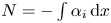 $N = -\int \alpha _i\,\textrm {d} x$. To avoid the significant computational cost associated with solving the spatial eigenvalue problem (2.11), the relation between the temporal and the spatial growth rates given by Gaster (Reference Gaster1962) is employed. This relation, commonly known as the Gaster transformation, can be expressed as follows:
 \begin{equation} \alpha_i |_{\omega_i = 0} ={-} \frac{\omega_i |_{\alpha_i = 0}}{c_g} + O(\omega_i |_{\alpha_i = 0}^2), \end{equation}
where 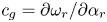 $c_g = \partial \omega _r / \partial \alpha _r$ denotes the group velocity of the disturbance. Although, in general, (6.1) is only accurate for convective instabilities with small temporal growth rates, it has been successfully applied by previous authors to the analysis of roughness-induced instabilities at high speed (see Groskopf et al. Reference Groskopf, Kloker, Stephani, Marxen and Iaccarino2010b; Groskopf & Kloker Reference Groskopf and Kloker2016). To verify its applicability to the temporal results presented here, figure 17 shows a comparison between spatial growth rates obtained by means of the Gaster transformation and spatial growth rates computed by solving the spatial eigenvalue problem for the leading wake instabilities. Good overall agreement is found for both roughness geometries, which renders the use of (6.1) a legitimate assumption for the purpose of this analysis. The biggest discrepancies encountered are for the cuboid varicose mode at
 $\lambda _x = 0.28\ \textrm {cm}$, corresponding to its particular region of development associated to small streamwise wavenumbers (high frequencies), as shown in figure 9
 $(a)$.
Spatial growth-rate evolution of the most unstable wake modes obtained by means of the Gaster transformation (6.1) (lines) and by solving the spatial eigenvalue problem (symbols):  $(a)$ cuboid;
 $(b)$ ramp.

Temporal stability computations make it possible to construct a stability diagram of the form  $\omega _i = \omega _i(\alpha _r,x)$, or
 $\omega _i = \omega _i(\lambda _x,x)$. By means of the Gaster transformation, the function
 $\alpha _i = \alpha _i(\lambda _x,x)$ can then be obtained. However, a meaningful evaluation of the integrated amplification factors requires a surface of the type
 $\alpha _i = \alpha _i(f,x)$, where
 $f = \omega _r/ (2 {\rm \pi})$ is the frequency of the disturbance, so that curves of
 $\alpha _i$ as a function of
 $x$ for a constant frequency can be integrated to obtain the evolution of
 $N$ associated to that frequency. Since
 $\omega _r$ is a solution of the temporal eigenvalue problem, it cannot be fixed constant a priori from the temporal results. Therefore, to obtain
 $\alpha _i = \alpha _i(f,x)$, an interpolation of the stability diagram
 $\alpha _i = \alpha _i(\lambda _x,x)$ must be employed. From the temporal stability calculations, the resulting frequency of the disturbances is found to be approximately proportional to
 $\alpha _r$. In addition, in the unstable region of the stability diagram, the range of frequencies spanned by each of the
 $\alpha _i = \alpha _i(x)$ curves for a constant
 $\lambda _x$ is very small in comparison with the range of frequencies over which the instabilities grow. These conditions favour the accuracy of the interpolation process. In this study, this procedure is performed by means of a cubic Hermite interpolation.
The spatial stability diagrams ( $\alpha _i = \alpha _i(f,x)$) obtained by means of the Gaster transformation for modes SIN1 and VCOS1 and for each of the roughness geometries under study are displayed in figure 18
 $(c$–
 $f)$. The shaded contours represent the spatial growth rate, and the contour lines superimposed illustrate the associated
 $N$-factor evolution. For comparison purposes, the diagrams shown in figure 18
 $(a{,}b)$ correspond to the instabilities developing in the smooth flat-plate boundary layer, which are obtained by means of LST for a given spanwise wavenumber. Figure 18
 $(a)$ depicts contours for the two-dimensional Mack-mode instability (
 $\beta = 0$), which is fully governed by high frequencies corresponding to second mode behaviour, whereas figure 18
 $(b)$ shows contours for an oblique Mack-mode instability with a spanwise wavenumber
 $\lambda _z = 0.4\ \textrm {cm}$, for which both Mack's first- and second-mode regions of development can be observed, respectively associated to the low- and high-frequency ranges. The integration of
 $N$ is started at the first streamwise station at which the modes become unstable. In the case of the wake instabilities, it is found that for certain frequencies the disturbances are already unstable at the first streamwise location analysed. Under these circumstances, a value of
 $N = 0$ is assumed at that location. This is a common procedure employed by other authors in similar analyses; see for instance Choudhari et al. (Reference Choudhari, Li, Chang, Norris and Edwards2013), De Tullio et al. (Reference De Tullio, Paredes, Sandham and Theofilis2013) and Theiss et al. (Reference Theiss, Hein, Ali and Radespiel2016). In addition, figure 19
 $(a)$ presents the streamwise evolution of the
 $N$-factor envelope (
 $N_{max}$) curves for each of the wake modes investigated. Here,
 $N_{max}$ denotes the maximum
 $N$-factor obtained at each streamwise position for all the different frequencies analysed. The particular frequency associated with
 $N_{max}$ at each location is shown in figure 19
 $(b)$.
Shaded contours of spatial growth rate ( $-\alpha _i$) and contour lines of
 $N$-factor as a function of frequency and streamwise position for
 $(a)$ two-dimensional Mack mode evolving in the smooth flat-plate boundary layer;
 $(b)$ oblique Mack mode (
 $\lambda _z = 0.4\ \textrm {cm}$) evolving in the smooth flat-plate boundary layer;
 $(c)$ cuboid, SIN1 mode;
 $(d)$ cuboid, VCOS1 mode;
 $(e)$ ramp, SIN1 mode;
 $(f)$ ramp, VCOS1 mode. Results for
 $(c$–
 $f)$ were obtained by means of the Gaster transformation (6.1).

 $(a)$ Streamwise evolution of the
 $N$-factor envelope (
 $N_{max}$) of the most unstable wake modes for each roughness geometry, obtained by employing the Gaster-transformed spatial growth rates;
 $(b)$ frequency associated to
 $N_{max}$ at each streamwise location for each of the curves shown in
 $(a)$.

These results complete the observations introduced before based on the temporal growth-rate evolution. The  $N$-factor envelopes confirm that the cuboid geometry favours the development of a varicose wake instability over a sinuous one, whereas the ramp configuration excites a sinuous disturbance more effectively than a varicose one. Close to the roughness element, the cuboidal geometry is more effective in promoting the linear growth of the dominant wake instability than the ramp-shaped one. However, the ramp element leads to a higher disturbance amplitude further downstream (
 $x > 0.2\ \textrm {m}$).
As shown in figure 18 $(d)$, two distinct regions of development for the cuboid-induced varicose instability can be identified. The frequency range for each of these regions is found to correlate well with that of Mack's first- and second-mode instabilities developing in the smooth flat plate. Although the biggest growth rates for this disturbance are located within the high-frequency band, the decay in this range is more accentuated than for the lower frequencies. As a result, the frequencies that govern the
 $N$-factor envelope for this mode are at first located in the upper range (
 $f \approx 280\ \textrm {kHz}$) and further downstream in the lower band (
 $f \approx 160\ \textrm {kHz}$), as shown in figure 19
 $(b)$. This leads to the abrupt change in the slope of the envelope curve at
 $x \approx 0.28\ \textrm {m}$. In accordance with the temporal stability results described above, this is the only instability for which two such different regions of excitation can be clearly observed in the stability diagram.
For the ramp-induced sinuous disturbance (see figure 18 $e$), the region of maximum growth is concentrated in the range of
 $f \approx 100\ \textrm {kHz}$ to
 $f \approx 160\ \textrm {kHz}$. This frequency band is associated with Mack's first-mode instabilities for the entire domain length. For higher frequencies (
 $f \approx 230\ \textrm {kHz}$ to
 $f \approx 270\ \textrm {kHz}$), a small enhancement of the spatial growth rates is observed starting at
 $x \approx 0.15\ \textrm {m}$. The same phenomenon is visible in the temporal growth rate curves shown in figure 16
 $(c)$ for
 $\lambda _x = 0.35\ \textrm {cm}$ and
 $\lambda _x = 0.42\ \textrm {cm}$. This behaviour correlates with the region of the stability diagram that overlaps with the development of Mack's second-mode instability in the flat-plate boundary layer. This observation further supports the argument of an interaction between the wake modes and the boundary-layer disturbances. In this case, however, this interaction does not have an impact on the
 $N$-factor envelope of the wake instability.
Although less relevant in terms of  $N_{max}$, the cuboid-induced sinuous disturbance and the ramp-induced varicose perturbation also show an influence from the boundary-layer instabilities. As in the ramp configuration, the sinuous mode associated to the cuboid geometry also features its maximum
 $N$ in the low-frequency band. For
 $x > 0.2\ \textrm {m}$, its spatial growth becomes approximately constant with respect to the streamwise position for
 $f < 130\ \textrm {kHz}$ (see figure 18
 $c$). This feature can also be observed in the temporal growth curves shown in figure 16
 $(a)$ for
 $\lambda _x = 0.7\ \textrm {cm}$ and
 $\lambda _x = 1\ \textrm {cm}$. This reduction in the decay of the growth rate of the instability is attributed to an interaction between the sinuous disturbance and Mack's first-mode instability. It has a significant impact on the evolution of the associated
 $N$-factor envelope, which shows a clear increase in slope in this region. Mode VCOS1 excited by the ramp roughness element is found to be rapidly stabilized at high frequencies, as shown in figure 18
 $(d)$. However, its growth rate is found to be influenced by both the first and second boundary-layer disturbances in the range
 $f \approx 100\ \textrm {kHz}$ to
 $f \approx 200\ \textrm {kHz}$. The interaction with Mack's first mode is noticeable starting at
 $x \approx 0.18\ \textrm {m}$, and the interaction with Mack's second mode is noticeable starting at
 $x \approx 0.33\ \textrm {m}$ (see also figure 16
 $d$).
6.3. Temporal growth-rate decomposition of the wake instabilities
This section describes the application of the temporal growth-rate decomposition introduced in § 3.1 to the evolution of the leading wake instabilities (modes VCOS1 and SIN1) excited by each roughness shape. Although the decomposition given by (3.9) consists of a large number of terms, only a small number of them are relevant for the physical interpretation of the problem studied. To illustrate which are the most relevant contributions, figures 20 and 21 present the decomposition obtained at  $x = 0.1\ \textrm {m}$ for the streamwise wavelengths considered in figures 7 and 8 for the cuboid and ramp configurations. The terms denoted by
 $\hat {P}_{s,2}$ and
 $\hat {P}_{s,3}$ respectively refer to the wall-normal and the spanwise contributions that constitute
 $\hat {P}_s$, i.e.
 \begin{equation} \hat{P}_{s,2} ={-} \int_{z^-}^{z^+} \int_{y^-}^{y^+} \bar{\rho} \langle \hat{v}, \hat{s} \rangle \dfrac{\partial \bar{T}}{\partial y}\, \textrm{d} y\, \textrm{d} z,\quad \hat{P}_{s,3} ={-} \int_{z^-}^{z^+} \int_{y^-}^{y^+} \bar{\rho} \langle \hat{w}, \hat{s} \rangle \dfrac{\partial \bar{T}}{\partial z}\, \textrm{d} y\, \textrm{d} z, \end{equation}
and the terms  $\hat {P}_{RS,12}$ and
 $\hat {P}_{RS,13}$ are the parts of the total Reynolds stress production term
 $\hat {P}_{RS}$ that respectively correspond to the stress components given by
 $\bar {\rho } \tilde {u} \tilde {v}$ and by
 $\bar {\rho } \tilde {u} \tilde {w}$, i.e.
 \begin{align} \hat{P}_{RS,12} ={-}\int_{z^-}^{z^+} \int_{y^-}^{y^+} \bar{\rho} \langle \hat{u}, \hat{v} \rangle \dfrac{\partial \bar{u}}{\partial y}\, \textrm{d} y\, \textrm{d} z,\quad \hat{P}_{RS,13} ={-} \int_{z^-}^{z^+} \int_{y^-}^{y^+} \bar{\rho} \langle \hat{u}, \hat{w} \rangle \dfrac{\partial \bar{u}}{\partial z}\, \textrm{d} y\, \textrm{d} z. \end{align}
Values of the most important contributions to the temporal growth-rate decomposition (3.9) for modes SIN1 and VCOS1 at  $x = 0.1\ \textrm {m}$ in the cuboid wake:
 $(a)$
 $\lambda _x = 0.325\ \textrm {cm}$;
 $(b)$
 $\lambda _x = 0.5\ \textrm {cm}$;
 $(c)$
 $\lambda _x = 1\ \textrm {cm}$. Each contribution is divided by the factor
 $2 \hat {E}$ (see (3.9)).

Values of the most important contributions to the temporal growth-rate decomposition (3.9) for modes SIN1 and VCOS1 at  $x = 0.1\ \textrm {m}$ in the ramp wake:
 $(a)$
 $\lambda _x = 0.35\ \textrm {cm}$;
 $(b)$
 $\lambda _x = 0.56\ \textrm {cm}$;
 $(c)$
 $\lambda _x = 0.86\ \textrm {cm}$. Each contribution is divided by the factor
 $2 \hat {E}$ (see (3.9)).

Only those terms which have a significant magnitude are included in figures 20 and 21; the contributions of the rest are found to be unimportant (of the order of  $\hat {P}_{Q}$ or below) in this case. The biggest contributions to the disturbance kinetic energy for both wake modes come from the production terms due to the relevant disturbance Reynolds stresses (
 $\hat {P}_{RS,12}$ and
 $\hat {P}_{RS,13}$), whereas the most important contributions to the potential energy of the disturbance are due to the transport of the entropy perturbation (
 $\hat {P}_{s,2}$ and
 $\hat {P}_{s,3}$). The production term due to the disturbance heat source (
 $\hat {P}_{Q}$) is in all cases one order of magnitude smaller than the
 $\hat {P}_s$ and the
 $\hat {P}_{RS}$ production terms, which is in good agreement with the findings of Chu (Reference Chu1965). It is worth emphasizing that, to the best of the authors’ knowledge, previous analyses found in the literature for isolated roughness elements in high-speed flows have only examined the evolution of the production of kinetic energy due to the disturbance Reynolds stresses. However, the current results show that the energy production terms associated to the transport of entropy fluctuations constitute an important contribution to the potential energy of the disturbance. Therefore, although their relative magnitude with respect to the production of kinetic energy due to the disturbance Reynolds stresses cannot be concluded from this formulation of the perturbation energy (see the reasons stated at the beginning of § 3), these results suggest that
 $\hat {P}_s$ might also play a significant role in high-speed flows. It is important to note that, within the definition of disturbance energy given by Chu (Reference Chu1965), the largest destabilizing (positive) contributions to the temporal growth rate of the wake modes are
 $\hat {P}_{s,2}$ and
 $\hat {P}_{s,3}$, while the largest stabilizing (negative) contribution is the dissipation of disturbance energy due to thermal conduction (
 $\hat {D}_k$). Nevertheless, since the terms
 $\hat {P}_{s,2}$,
 $\hat {P}_{s,3}$ and
 $\hat {D}_k$ originate from a different governing equation than the terms
 $\hat {P}_{RS,12}$,
 $\hat {P}_{RS,13}$ and
 $\hat {D}_\mu$, it is not possible to conclude which contributions are actually larger in practice, since different choices of the multipliers that constitute the disturbance energy formulation alter the relative magnitudes of these sets of terms.
For the cuboid geometry, the decomposition reveals a difference in the source of disturbance energy for the varicose mode at  $x = 0.1\ \textrm {m}$ and
 $\lambda _x = 0.325\ \textrm {cm}$ with respect to the other two wavelengths. As can be noticed, at this wavelength, the growth rate of mode VCOS1 is dominated by the wall-normal production terms (
 $\hat {P}_{s,2}$ and
 $\hat {P}_{RS,12}$), whereas for
 $\lambda _x = 0.5\ \textrm {cm}$ and
 $\lambda _x = 1\ \textrm {cm}$ it is governed by the spanwise production contributions (
 $\hat {P}_{s,3}$ and
 $\hat {P}_{RS,13}$). This reflects once again the occurrence of two different manifestations of the varicose disturbance depending on the streamwise wavelength (or frequency in the spatial case), as discussed previously.
6.3.1. Streamwise evolution of the temporal growth-rate decomposition
With the aim of investigating the particular features found in the growth-rate evolution of the SIN1 and VCOS1 modes, the streamwise evolution of the temporal growth-rate decomposition for each of the two disturbances is presented in figures 22 and 23 for the cuboid configuration and in figures 24 and 25 for the ramp. For the cuboidal geometry, it is observed that immediately behind the trailing-edge recirculation bubble, the energy of both instabilities is governed by the wall-normal production terms  $\hat {P}_{s,2}$ and
 $\hat {P}_{RS,12}$. This implies that in this region the modes extract their energy from the wall-normal base-flow gradients. A short distance further downstream, depending on the streamwise wavelength, the wall-normal production terms rapidly decrease and the disturbance energy is transferred to the spanwise production contributions
 $\hat {P}_{s,3}$ and
 $\hat {P}_{RS,13}$, bringing the wall-normal terms to a negative (stabilizing) energy contribution for most of the studied wavelengths. After this first exchange of energy from the wall-normal to the spanwise contributions, the leading term
 $\hat {P}_{s,3}$ reaches a maximum and begins to decrease at an approximately constant rate. In parallel, the wall-normal terms continue to decrease, which enhances their stabilizing effect. However, after a given distance downstream, the wall-normal production terms start to rise again in most of the cases. This rise is accompanied by an acceleration in the rate of decrease of the spanwise terms, so that there is reciprocal evolution between
 $\hat {P}_{s,2}$ and
 $\hat {P}_{s,3}$ and between
 $\hat {P}_{RS,12}$ and
 $\hat {P}_{RS,13}$. This implies that another energy transfer begins to take place along the roughness wake, in this case from spanwise to wall-normal production terms, at a slower pace than the first one. This second exchange can be observed for the sinuous mode for all three wavelengths: for
 $\lambda _x = 0.325\ \textrm {cm}$ and
 $\lambda _x = 0.5\ \textrm {cm}$, it starts at
 $x \approx 0.18\ \textrm {m}$ and continues until the end of the domain; for
 $\lambda _x = 1\ \textrm {cm}$, it starts immediately after the first exchange (
 $x \approx 0.13\ \textrm {m}$). In the case of the varicose mode, it can also be observed for
 $\lambda _x = 0.5\ \textrm {cm}$ (starting at
 $x \approx 0.35\ \textrm {m}$) and for
 $\lambda _x = 1\ \textrm {cm}$ (starting at
 $x \approx 0.14\ \textrm {m}$) within the studied domain length.
Streamwise evolution of the main production  $(a\text {--}c)$ and dissipation
 $(d\text {--}f)$ terms for mode SIN1 developing in the cuboidal roughness wake at three different wavelengths:
 $(a{,}d)$
 $\lambda _x = 0.325\ \textrm {cm}$;
 $(b{,}e)$
 $\lambda _x = 0.5\ \textrm {cm}$;
 $(c{,}f)$
 $\lambda _x = 1\ \textrm {cm}$.

Streamwise evolution of the main production  $(a\text {--}c)$ and dissipation
 $(d\text {--}f)$ terms for mode VCOS1 developing in the cuboidal roughness wake at three different wavelengths:
 $(a{,}d)$
 $\lambda _x = 0.325\ \textrm {cm}$;
 $(b{,}e)$
 $\lambda _x = 0.5\ \textrm {cm}$;
 $(c{,}f)$
 $\lambda _x = 1\ \textrm {cm}$.

Streamwise evolution of the main production  $(a\text {--}c)$ and dissipation
 $(d\text {--}f)$ terms for mode SIN1 corresponding to the ramp geometry at three different wavelengths:
 $(a{,}d)$
 $\lambda _x = 0.35\ \textrm {cm}$;
 $(b{,}e)$
 $\lambda _x = 0.56\ \textrm {cm}$;
 $(c{,}f)$
 $\lambda _x = 0.86\ \textrm {cm}$.

Streamwise evolution of the main production  $(a\text {--}c)$ and dissipation
 $(d\text {--}f)$ terms for mode VCOS1 corresponding to the ramp geometry at three different wavelengths:
 $(a{,}d)$
 $\lambda _x = 0.35\ \textrm {cm}$;
 $(b{,}e)$
 $\lambda _x = 0.56\ \textrm {cm}$;
 $(c{,}f)$
 $\lambda _x = 0.86\ \textrm {cm}$.

From the energy signature of both cuboid-induced modes at  $\lambda _x = 1\ \textrm {cm}$, it is clear that this second energy transfer mechanism brings the spanwise production terms asymptotically to approximately zero. Hence, it does not lead to stabilizing contributions associated to the work done through the spanwise base-flow gradients. This implies that the wake instabilities in this condition become governed only by the energy production processes linked to the wall-normal base-flow gradients. This is an inherent characteristic of the energy budget of boundary-layer modes that develop in a smooth flat-plate boundary layer in which no spanwise base-flow gradients exist. In accordance with this observation, it has been found that the occurrence of the second energy exchange correlates with streamwise stations at which the amplitude of the eigenfunctions associated with the wake instabilities VCOS1 and SIN1 begins to increase also in the boundary layer outside of the roughness wake, with amplitude distributions that are equivalent to the Mack-mode instabilities shown in figure 12. This provides evidence that there is an interaction between the wake instabilities and the boundary-layer modes which influences the growth-rate evolution of the wake disturbances. As described in § 6.4, this interaction can be interpreted as a continuous synchronization between the wake modes and the boundary-layer modes.
For the ramp-induced instabilities, the disturbance energy near the roughness trailing edge is also governed by the wall-normal energy production quantities ( $\hat {P}_{s,2}$ and
 $\hat {P}_{RS,12}$). A clear difference between the energy signature of mode SIN1 for both roughness geometries is that, for the ramp element, the first transfer of energy from the wall-normal to the spanwise production terms takes place over a longer streamwise distance. This is particularly evident for the cases with
 $\lambda _x = 0.56\ \textrm {cm}$ and
 $\lambda _x = 0.86\ \textrm {cm}$, for which the spanwise term
 $\hat {P}_{s,3}$ does not become the dominant contribution until approximately halfway into the domain length. Therefore, the wall-normal base-flow gradients remain responsible for the excitation of the leading disturbance in the ramp-induced wake for a long distance downstream. Additionally, for
 $\lambda _x = 0.35\ \textrm {cm}$, the disturbance energy evolution confirms that the sinuous mode is strongly influenced by the presence of Mack-mode instabilities starting at
 $x \approx 0.15\ \textrm {m}$, as evidenced by the sharp rise in the term
 $\hat {P}_{s,2}$ and the sharp decrease in the term
 $\hat {P}_{s,3}$. This explains the rise in growth rate that can be observed in figure 16
 $(c)$ for this wavelength. In this case, however, the effect of the synchronization does not last until the end of the domain. Downstream of
 $x \approx 0.2\ \textrm {m}$, a third energy exchange takes place and the mode recovers the behaviour of a pure wake instability, eventually becoming governed by the spanwise base-flow gradients in a similar way to the other two cases, for which no sign of a synchronization is present.
Significant differences are also found between the energy balances of the varicose mode in the two roughness configurations. For the ramp geometry, the first energy transfer between wall-normal and spanwise terms occurs at a much shorter distance behind the roughness trailing edge. Similarly, the second energy exchange, which leads to a transformation of the instability towards a hybrid wake–boundary-layer disturbance, takes place further upstream and is encountered within the domain length for all three streamwise wavelengths analysed. For  $\lambda _x = 0.35\ \textrm {cm}$, it begins to occur at
 $x \approx 0.17\ \textrm {m}$, for
 $\lambda _x = 0.56\ \textrm {cm}$ at
 $x \approx 0.12\ \textrm {m}$ and for
 $\lambda _x = 0.86\ \textrm {cm}$ at
 $x \approx 0.09\ \textrm {m}$. This explains the fluctuations in the growth rate encountered for
 $\lambda _x = 0.35\ \textrm {cm}$ and
 $\lambda _x = 0.56\ \textrm {cm}$, as shown in figure 16
 $(d)$. Furthermore, since for
 $\lambda _x = 0.86\ \textrm {cm}$ the synchronization with the boundary-layer modes begins upstream of
 $x = 0.1\ \textrm {m}$, the amplitude function of the varicose mode at these conditions (displayed in figure 11
 $c$) already shows a non-zero amplitude in the boundary layer at the sides of the roughness wake.
The contribution of the disturbance energy dissipation terms follows a similar trend for all the different cases analysed for each roughness geometry. The magnitude of the dissipative energy terms is maximum immediately behind the roughness trailing edge separation region and undergoes a very rapid decrease in a very short distance downstream. This decrease defines the streamwise location of maximum growth rate for each streamwise wavelength. Further downstream, both terms progressively decrease in magnitude. Their evolution is also found to be sensitive to interaction with boundary-layer disturbances.
Finally, it is important to note that no significant differences are observed between the disturbance energy extraction mechanisms of the two types of wake instabilities, only between the streamwise ranges over which the energy exchanges occur. The same finding is reported by Theiss et al. (Reference Theiss, Hein, Ali and Radespiel2016) for the streamwise evolution of the Reynolds stress production terms  $\hat {P}_{RS,12}$ and
 $\hat {P}_{RS,13}$ near the trailing edge of different roughness geometries mounted on the forebody of a reentry capsule. For all the cases analysed by Theiss et al. (Reference Theiss, Hein, Ali and Radespiel2016), the wall-normal contribution (
 $\hat {P}_{RS,12}$) was also found to be larger than the spanwise one for both wake instabilities in the immediate vicinity of the roughness elements. In addition, the current results show that the streamwise evolution of the growth rate of the varicose and sinuous instabilities is not uniquely governed by the energy production terms associated to the base-flow gradients along a single spatial direction. Rather, the production terms linked to the gradients along
 $y$ are the leading contributions for certain streamwise regions, whereas the terms related to the gradients along
 $z$ are the most important contributions for other regions. It is observed that base-flow gradients along both the wall-normal and spanwise directions play an important role in the evolution of both varicose and sinuous disturbances.
6.4. Synchronism between wake instabilities and boundary-layer modes
This last section is devoted to illustrating a synchronization process between the wake-induced disturbances and the boundary-layer instabilities. Figure 26 depicts the magnitude of the streamwise velocity amplitude function of the SIN1 and VCOS1 instabilities excited by the cuboid roughness element at four different streamwise locations for  $\lambda _x = 0.5\ \textrm {cm}$. As can be observed, after a given streamwise distance, the amplitude of the wake modes begins to increase in the regions located at the undisturbed boundary layer outside of the roughness wake, in a very similar way to the oblique Mack-mode instabilities shown in figure 12 (the same behaviour is observed for the ramp geometry, not shown here). This provides evidence of an interaction between the wake instability modes and Mack's mode family. For the same configuration, figure 27 shows the streamwise evolution of the phase speed (
 $c_{ph} = \omega _r/\alpha _r$) of the leading sinuous and varicose modes as well as of different instabilities located along the Mack-mode branch, namely, modes M2D, MO3, MO4 and MO7, already shown in figure 12. The phase speed of mode SIN1 begins to match the phase speed of the Mack-mode instabilities starting at
 $x \approx 0.2\ \textrm {m}$. This coincides with the location at which the eigenfunction of the sinuous disturbance starts to develop amplitude in the boundary layer at the sides of the roughness wake. The same is encountered for the varicose mode, for which the match in phase speeds begins significantly further downstream, approximately at
 $x = 0.35\ \textrm {m}$, once again in good agreement with the location of the change in its amplitude function according to figure 26. Since the Mack-mode instability manifests itself as a continuous branch in the 2D-LST spectrum, this means that there is a continuous synchronization between the wake instability modes and the Mack modes. Such a synchronization mechanism was suggested by De Tullio & Sandham (Reference De Tullio and Sandham2015) for the excitation of varicose modes, based on DNS results for a very similar cuboidal roughness configuration. In this work, this phenomenon is observed for both sinuous and varicose disturbances and for the two different roughness geometries investigated, bringing further weight to the importance of this mechanism in roughness-induced transition.
Normalized magnitude of the streamwise velocity amplitude function of modes SIN1  $(a{,}c{,}e{,}g)$ and VCOS1
 $(b{,}d{,}f{,}h)$ for the cuboid geometry at
 $\lambda _x = 0.5\ \textrm {cm}$ and at four different streamwise locations:
 $(a{,}b)$
 $x = 0.15\ \textrm {m}$;
 $(c{,}d)$
 $x = 0.2\ \textrm {m}$;
 $(e{,}f)$
 $x = 0.27\ \textrm {m}$;
 $(g{,}h)$
 $x = 0.38\ \textrm {m}$. Contour levels range between 0 and
 $0.5 |\hat {u}| / \max (|\hat {u}|)$ to favour the visualization of structures developing at the sides of the roughness wake.

Streamwise evolution of the non-dimensional phase speed of different instability modes developing behind the cuboid roughness element for  $\lambda _x = 0.5\ \textrm {cm}$. Solid and dashed lines denote the leading wake instability modes (VCOS1 and SIN1), and dash–dot lines with symbols correspond to different Mack instability modes (M2D, MO3, MO4 and MO7).

Under the synchronization process, the wake instabilities progressively transform into hybrid modes that develop in the roughness wake as well as at the surrounding boundary layer, in the same way as the instabilities belonging to the Mack-mode family that are modulated by the roughness wake. This transformation is reflected in the energy decomposition of the sinuous and varicose modes. Recalling the streamwise evolution of the temporal growth-rate decomposition terms (figures 22 and 23), it can be noticed that there is a close relationship between the location at which the synchronization starts and the position at which the leading production terms change their behaviour. For  $\lambda _x = 0.5\ \textrm {cm}$, the location at which the term
 $\hat {P}_{s,2}$ starts to grow after the first energy exchange is approximately
 $x = 0.2\ \textrm {m}$ for mode SIN1 and
 $x = 0.35\ \textrm {m}$ for mode VCOS1, which precisely coincide with the locations at which their respective phase speeds match those of the Mack-mode branch. Downstream of these streamwise stations, the energy decomposition of modes SIN1 and VCOS1 is expected to become closer to that of the Mack-mode disturbances.
The temporal growth-rate budget for mode M2D is presented in figure 28. For comparison purposes, the decomposition based on LST for the two-dimensional Mack mode ( $\beta = 0$) developing in a smooth flat-plate boundary layer is also included. In this case, the decomposition is evaluated by setting all base-flow spanwise derivatives to zero, so that only wall-normal production terms remain. As can be observed, the energy of the 2D-LST Mack mode is governed by the wall-normal production terms. Although its amplitude function is strongly modulated by the presence of the roughness, the energy signature of the 2D-LST Mack mode is still very close to the LST one, for which no spanwise production terms exist. This implies that the same is also true for its growth-rate evolution. These results confirm that, when the synchronization starts, the disturbance energy decomposition of modes SIN1 and VCOS1 begins to approach the energy signature of the Mack-mode instabilities, namely, spanwise terms (
 $\hat {P}_{s,3}$ and
 $\hat {P}_{RS,13}$) decreasing towards zero and wall-normal terms (
 $\hat {P}_{s,2}$ and
 $\hat {P}_{RS,12}$) rising. As the wake perturbations begin to develop amplitude in the boundary layer outside of the roughness wake, there is a redistribution of the disturbance energy from the spanwise components to the wall-normal ones.
Streamwise evolution of the temporal growth-rate decomposition for the two-dimensional Mack-mode instability (M2D) found in the cuboidal roughness element wake for  $\lambda _x = 0.5\ \textrm {cm}$:
 $(a)$ production terms;
 $(b)$ dissipation terms. Results for the two-dimensional Mack mode developing in the corresponding smooth flat-plate boundary layer, obtained by means of LST, are also included for comparison.

This is one mechanism by which the wake instabilities change their properties along the wake, and which has a direct impact on their amplification rates. It is therefore important to account for this phenomenon in the modelling of the linear stages of roughness-induced transition in conditions where wake and boundary-layer instabilities coexist.
7. Conclusions
The instabilities induced by an isolated roughness element in a Mach 6 flat-plate boundary layer have been investigated using two-dimensional local linear stability theory (2D-LST). The decomposition of the temporal growth rate derived by Weder et al. (Reference Weder, Gloor and Kleiser2015) from the disturbance energy equation developed by Chu (Reference Chu1965) has been extended for the first time to base flows that depend on two spatial directions and has been applied to the instabilities developing in the wake behind a discrete roughness element. These analyses have revealed that the roughness-induced wake instabilities extract most of their potential energy from the transport of the disturbance entropy across the wall-normal and the spanwise temperature gradients of the base flow. Similarly, most of their kinetic energy originates from the work done by the disturbance Reynolds stresses against the wall-normal and the spanwise velocity shear layers present in the base flow. The growth rate of the wake instabilities has been found to be strongly influenced by the boundary-layer disturbances developing on the flat plate, which become modulated by the presence of the roughness element. In particular, evidence has been observed of a continuous synchronization between the wake instabilities and the boundary-layer modes which resembles the second mechanism hypothesized by De Tullio & Sandham (Reference De Tullio and Sandham2015) for the excitation of varicose wake modes. This mechanism transforms the energy signature of the wake instabilities and leads to an enhancement of their amplification rate far downstream of the roughness element, ultimately increasing the associated integrated amplification factors.
Two different roughness geometries have been considered, with a height equal to 0.59 times the local boundary-layer thickness, leading to a roughness Reynolds number of 330. The first is a sharp-edged cuboidal element with a square planform shape, and the second is a three-dimensional sharp-edged ramp geometry. The roughness elements induce a pair of counter-rotating streamwise vortices that, through the lift-up mechanism, generate a wake flow structure consisting of a central low-velocity streak surrounded by two high-velocity streaks. The strong velocity gradient established at the interface between the low-velocity streak and the outer flow leads to a three-dimensional high-shear layer that supports the growth of different instabilities. The evolution of the streamwise vorticity magnitude along the roughness wake indicates that the cuboidal element induces a stronger counter-rotating vortex pair than the ramp. However, the smaller spanwise extent and the lateral angle present in the ramp geometry result in counter-rotating vortices that are closer to each other, generating a narrower and taller low-velocity streak.
Temporal 2D-LST computations have been performed along the roughness wake for the range of the most unstable streamwise wavelengths. The results illustrate that both wake instability modes and boundary-layer modes coexist in the stability spectrum for all conditions investigated. The wake modes consist of varicose and sinuous deformations of the low-velocity streak that characterizes the wake flow-field, whereas the boundary-layer modes are families of Mack's first- or second-mode instabilities developing in the flat-plate boundary layer that are modulated by the roughness wake. Two leading instability modes have been distinguished for each case, respectively corresponding to the most unstable sinuous (SIN1) and varicose (VCOS1) instabilities. The amplitude functions of these modes reveal that their regions of development are mainly concentrated in the three-dimensional high-shear layer that surrounds the central streak. Integrated amplification factors obtained by means of a Gaster transformation of the temporal stability results show that the cuboidal roughness element excites the varicose instability more strongly than the sinuous one, whereas the ramp geometry is found to favour the growth of the sinuous mode over the varicose one. Near the roughness element, the cuboidal configuration is more effective in promoting the linear growth of the dominant wake instability mode than the ramp-shaped one. Further downstream, however, the ramp-induced wake leads to a higher disturbance amplitude.
The derived temporal growth-rate decomposition provides an additional layer of information for understanding the streamwise evolution of the wake instabilities. The results obtained in this study show that the most important contributions to the disturbance potential energy come from the transport of disturbance entropy across the temperature shear layers ( $\hat {P}_{s}$), while the largest contributions to the disturbance kinetic energy are produced by the work done by the Reynolds stresses against the velocity shear layers (
 $\hat {P}_{RS}$). Previous studies in the literature on high-speed roughness-induced transition have mainly analysed the Reynolds stress production terms. However, the current results indicate that the production of potential energy due to entropy fluctuations might also play a significant role in high-speed flows. Whether the terms related to the potential disturbance energy have a larger magnitude in practice than those related to the kinetic energy cannot be concluded from the disturbance energy definition of Chu (Reference Chu1965), owing to the non-uniqueness of the multiplicative factors on which the formulation is based. On the other hand, the obtained decompositions show that in practice, for the disturbance energy analysis of roughness wake instabilities developing in hypersonic flow in a configuration like the one presented in this work, it is sufficient to pay attention to the production terms
 $\hat {P}_{s}$ and
 $\hat {P}_{RS}$, and to the dissipation terms
 $\hat {D}_\mu$ and
 $\hat {D}_k$. The remaining terms make small contributions which are not significant.
The streamwise evolution of the disturbance energy decomposition reveals that both wake instabilities are dominated by the wall-normal production terms in the vicinity of the roughness element and that the energy is progressively transferred to the spanwise production terms further downstream. The rate at which this transfer takes place is found to be faster for the cuboidal element. A relevant finding is that no significant differences are observed between the energy extraction mechanisms of the two types of wake instability, only between the ranges over which the energy transfers occur. Therefore, both wall-normal and spanwise base-flow gradients play a major role in the excitation of both sinuous and varicose instabilities.
For many of the conditions investigated, the amplitude of the wake modes is also found to grow in the boundary layer at the sides of the roughness wake, resembling the amplitude function of Mack-mode instabilities. This behaviour correlates with changes in the evolution of the energy production terms – more specifically, with downstream locations at which the wall-normal production terms begin to rise and the spanwise terms accelerate their rate of decrease. An analysis of the phase speed evolution of different instabilities shows that this behaviour also correlates with the location at which the phase speed of the wake modes matches that of the Mack-mode instabilities. These observations provide evidence that there is a continuous synchronization between the wake instabilities and the boundary-layer modes. When this synchronization begins to take place, the energy signature of the wake modes changes its behaviour and starts to become similar to that of Mack-mode disturbances. This phenomenon has important implications for the growth-rate evolution of the wake instabilities, in some cases enhancing their amplification rate or decreasing the rate of decay of the perturbations. Such a mechanism for the excitation of wake modes was suggested by De Tullio & Sandham (Reference De Tullio and Sandham2015) for the case of varicose disturbances behind a cuboidal roughness element, according to DNS-based analyses. In this work, it has been observed for both sinuous and varicose instabilities induced by two different roughness geometries, which brings further evidence that this phenomenon could play a crucial role in roughness-induced transition.
Finally, it is worth mentioning that the results presented in this work correspond to a cold wall condition. Under adiabatic wall conditions, the resulting base-flow heating is expected to have an impact on the interaction between the boundary-layer modes and the wake instabilities through a stabilization of the second Mack mode, which is known to be highly tuned with the local boundary-layer thickness. As reported by De Tullio & Sandham (Reference De Tullio and Sandham2015), wake modes which undergo a synchronism with boundary-layer instabilities for frequencies associated to second-Mack-mode behaviour are expected to be more influenced by changes in the thermal wall condition.
Acknowledgements
The authors would like to thank the reviewers for the constructive criticism provided in order to improve this article. The authors would also like to thank Prof. Miguel Hermanns for kindly sharing the computational routines that implement the finite-difference discretization employed in this work.
Funding
Part of this work has received funding from the European Union's Horizon 2020 research and innovation programme under the Marie Skłodowska-Curie grant agreement no. 675008.
Declaration of interests
The authors report no conflict of interest.
Appendix A. Linearized perturbation equations
For a steady and streamwise parallel base flow ( $\bar {\boldsymbol {q}} = \bar {\boldsymbol {q}}(y,z)$) with three-dimensional unsteady perturbations (
 $\tilde {\boldsymbol {q}} = \tilde {\boldsymbol {q}}(x,y,z,t)$), the linearized disturbance equations for a calorically perfect gas can be expressed as follows:
 \begin{gather} \dfrac{\partial \tilde{\rho}}{\partial t} + \bar{\rho} \left( \dfrac{\partial \tilde{u}}{\partial x} + \dfrac{\partial \tilde{v}}{\partial y} + \dfrac{\partial \tilde{w}}{\partial z} \right) + \tilde{\rho} \left( \dfrac{\partial \bar{v}}{\partial y} + \dfrac{\partial \bar{w}}{\partial z} \right) + \bar{u} \dfrac{\partial \tilde{\rho}}{\partial x} + \bar{v} \dfrac{\partial \tilde{\rho}}{\partial y} + \bar{w} \dfrac{\partial \tilde{\rho}}{\partial z} + \tilde{v} \dfrac{\partial \bar{\rho}}{\partial y} + \tilde{w} \dfrac{\partial \bar{\rho}}{\partial z} = 0, \end{gather}
 \begin{gather} \bar{\rho} \left( \dfrac{\partial \tilde{u}}{\partial t} + \bar{u} \dfrac{\partial \tilde{u}}{\partial x} + \bar{v} \dfrac{\partial \tilde{u}}{\partial y} + \bar{w} \dfrac{\partial \tilde{u}}{\partial z} + \tilde{v} \dfrac{\partial \bar{u}}{\partial y} + \tilde{w} \dfrac{\partial \bar{u}}{\partial z} \right) + \tilde{\rho} \left( \bar{v} \dfrac{\partial \bar{u}}{\partial y} + \bar{w} \dfrac{\partial \bar{u}}{\partial z} \right) \nonumber\\ + \frac{1}{\gamma M^2} \left( \bar{T} \dfrac{\partial \tilde{\rho}}{\partial x} + \bar{\rho} \dfrac{\partial \tilde{T}}{\partial x} \right) - \frac{1}{Re} \left\{ \bar{\lambda} \left( \dfrac{\partial^2 \tilde{u}}{\partial x^2} + \dfrac{\partial^2 \tilde{v}}{\partial x \partial y} + \dfrac{\partial^2 \tilde{w}}{\partial x \partial z} \right) \right.\nonumber\\ + \bar{\mu} \left( 2 \dfrac{\partial^2 \tilde{u}}{\partial x^2} + \dfrac{\partial^2 \tilde{v}}{\partial x \partial y} + \dfrac{\partial^2 \tilde{u}}{\partial y^2} + \dfrac{\partial^2 \tilde{u}}{\partial z^2} + \dfrac{\partial^2 \tilde{w}}{\partial x \partial z} \right) + \dfrac{\textrm{d} \bar{\lambda}}{\textrm{d} \bar{T}} \dfrac{\partial \tilde{T}}{\partial x} \left(\dfrac{\partial \bar{v}}{\partial y} + \dfrac{\partial \bar{w}}{\partial z} \right)\nonumber\\ + \dfrac{\textrm{d} \bar{\mu}}{\textrm{d} \bar{T}} \left[ \tilde{T} \left(\dfrac{\partial^2 \bar{u}}{\partial y^2} + \dfrac{\partial^2 \bar{u}}{\partial z^2} \right) + \dfrac{\partial \bar{T}}{\partial y} \left( \dfrac{\partial \tilde{v}}{\partial x} + \dfrac{\partial \tilde{u}}{\partial y} \right) + \dfrac{\partial \tilde{T}}{\partial y} \dfrac{\partial \bar{u}}{\partial y} \right.\nonumber\\ \left. \left. + \dfrac{\partial \bar{T}}{\partial z} \left( \dfrac{\partial \tilde{u}}{\partial z} + \dfrac{\partial \tilde{w}}{\partial x} \right) + \dfrac{\partial \tilde{T}}{\partial z} \dfrac{\partial \bar{u}}{\partial z} \right] + \dfrac{\textrm{d}^2 \bar{\mu}}{\textrm{d} \bar{T}^2} \tilde{T} \left( \dfrac{\partial \bar{T}}{\partial y} \dfrac{\partial \bar{u}}{\partial y} + \dfrac{\partial \bar{T}}{\partial z} \dfrac{\partial \bar{u}}{\partial z} \right) \right\} = 0, \end{gather}
 \begin{gather} \bar{\rho} \left( \dfrac{\partial \tilde{v}}{\partial t} + \bar{u} \dfrac{\partial \tilde{v}}{\partial x} + \bar{v} \dfrac{\partial \tilde{v}}{\partial y} + \bar{w} \dfrac{\partial \tilde{v}}{\partial z} + \tilde{v} \dfrac{\partial \bar{v}}{\partial y} + \tilde{w} \dfrac{\partial \bar{v}}{\partial z} \right) + \tilde{\rho} \left( \bar{v} \dfrac{\partial \bar{v}}{\partial y} + \bar{w} \dfrac{\partial \bar{v}}{\partial z} \right)\nonumber\\ + \frac{1}{\gamma M^2} \left( \bar{T} \dfrac{\partial \tilde{\rho}}{\partial y} + \tilde{T} \dfrac{\partial \bar{\rho}}{\partial y} + \bar{\rho} \dfrac{\partial \tilde{T}}{\partial y} + \tilde{\rho} \dfrac{\partial \bar{T}}{\partial y} \right) - \frac{1}{Re} \left\{ \bar{\lambda} \left( \dfrac{\partial^2 \tilde{u}}{\partial x \partial y} + \dfrac{\partial^2 \tilde{v}}{\partial y^2} + \dfrac{\partial^2 \tilde{w}}{\partial y \partial z} \right) \right.\nonumber\\ + \bar{\mu} \left( \dfrac{\partial^2 \tilde{u}}{\partial x \partial y} + \dfrac{\partial^2 \tilde{v}}{\partial x^2} + 2 \dfrac{\partial^2 \tilde{v}}{\partial y^2} + \dfrac{\partial^2 \tilde{v}}{\partial z^2} + \dfrac{\partial^2 \tilde{w}}{\partial y \partial z} \right) + \dfrac{\textrm{d} \bar{\lambda}}{\textrm{d} \bar{T}} \left[ \dfrac{\partial \bar{T}}{\partial y} \left( \dfrac{\partial \tilde{u}}{\partial x} + \dfrac{\partial \tilde{v}}{\partial y} + \dfrac{\partial \tilde{w}}{\partial z} \right) \right.\nonumber\\ \left. + \dfrac{\partial \tilde{T}}{\partial y} \left(\dfrac{\partial \bar{v}}{\partial y} + \dfrac{\partial \bar{w}}{\partial z} \right) + \tilde{T} \left( \dfrac{\partial^2 \bar{v}}{\partial y^2} + \dfrac{\partial^2 \bar{w}}{\partial y \partial z} \right) \right] + \dfrac{\textrm{d} \bar{\mu}}{\textrm{d} \bar{T}} \left[ 2 \dfrac{\partial \bar{T}}{\partial y} \dfrac{\partial \tilde{v}}{\partial y} + 2 \dfrac{\partial \tilde{T}}{\partial y} \dfrac{\partial \bar{v}}{\partial y} \right.\nonumber\\ \left. + \tilde{T} \left( 2 \dfrac{\partial^2 \bar{v}}{\partial y^2} + \dfrac{\partial^2 \bar{v}}{\partial z^2} + \dfrac{\partial^2 \bar{w}}{\partial y \partial z} \right) + \dfrac{\partial \tilde{T}}{\partial x} \dfrac{\partial \bar{u}}{\partial y} + \dfrac{\partial \bar{T}}{\partial z} \left( \dfrac{\partial \tilde{v}}{\partial z} + \dfrac{\partial \tilde{w}}{\partial y} \right) + \dfrac{\partial \tilde{T}}{\partial z} \left( \dfrac{\partial \bar{v}}{\partial z} + \dfrac{\partial \bar{w}}{\partial y} \right) \right]\nonumber\\ \left. + \dfrac{\textrm{d}^2 \bar{\lambda}}{\textrm{d} \bar{T}^2} \tilde{T} \dfrac{\partial \bar{T}}{\partial y} \left( \dfrac{\partial \bar{v}}{\partial y} + \dfrac{\partial \bar{w}}{\partial z} \right) + \dfrac{\textrm{d}^2 \bar{\mu}}{\textrm{d} \bar{T}^2} \tilde{T} \left[ 2 \dfrac{\partial \bar{T}}{\partial y} \dfrac{\partial \bar{v}}{\partial y} + \dfrac{\partial \bar{T}}{\partial z} \left( \dfrac{\partial \bar{v}}{\partial z} + \dfrac{\partial \bar{w}}{\partial y} \right) \right] \right\} = 0, \end{gather}
 \begin{gather} \bar{\rho} \left( \dfrac{\partial \tilde{w}}{\partial t} + \bar{u} \dfrac{\partial \tilde{w}}{\partial x} + \bar{v} \dfrac{\partial \tilde{w}}{\partial y} + \bar{w} \dfrac{\partial \tilde{w}}{\partial z} + \tilde{v} \dfrac{\partial \bar{w}}{\partial y} + \tilde{w} \dfrac{\partial \bar{w}}{\partial z} \right) + \tilde{\rho} \left( \bar{v} \dfrac{\partial \bar{w}}{\partial y} + \bar{w} \dfrac{\partial \bar{w}}{\partial z} \right) \nonumber\\ + \frac{1}{\gamma M^2} \left( \bar{T} \dfrac{\partial \tilde{\rho}}{\partial z} + \tilde{T} \dfrac{\partial \bar{\rho}}{\partial z} + \bar{\rho} \dfrac{\partial \tilde{T}}{\partial z} + \tilde{\rho} \dfrac{\partial \bar{T}}{\partial z} \right) - \frac{1}{Re} \left\{ \bar{\lambda} \left( \dfrac{\partial^2 \tilde{u}}{\partial x \partial z} + \dfrac{\partial^2 \tilde{v}}{\partial y \partial z} + \dfrac{\partial^2 \tilde{w}}{\partial z^2} \right) \right.\nonumber\\ + \bar{\mu} \left( \dfrac{\partial^2 \tilde{u}}{\partial x \partial z} + \dfrac{\partial^2 \tilde{v}}{\partial y \partial z} + \dfrac{\partial^2 \tilde{w}}{\partial x^2} + \dfrac{\partial^2 \tilde{w}}{\partial y^2} + 2 \dfrac{\partial^2 \tilde{w}}{\partial z^2} \right) + \dfrac{\textrm{d} \bar{\lambda}}{\textrm{d} \bar{T}} \left[ \dfrac{\partial \bar{T}}{\partial z} \left( \dfrac{\partial \tilde{u}}{\partial x} + \dfrac{\partial \tilde{v}}{\partial y} + \dfrac{\partial \tilde{w}}{\partial z} \right) \right.\nonumber\\ \left. + \dfrac{\partial \tilde{T}}{\partial z} \left(\dfrac{\partial \bar{v}}{\partial y} + \dfrac{\partial \bar{w}}{\partial z} \right) + \tilde{T} \left( \dfrac{\partial^2 \bar{v}}{\partial y \partial z} + \dfrac{\partial^2 \bar{w}}{\partial z^2} \right) \right] + \dfrac{\textrm{d} \bar{\mu}}{\textrm{d} \bar{T}} \left[ 2 \dfrac{\partial \bar{T}}{\partial z} \dfrac{\partial \tilde{w}}{\partial z} + 2 \dfrac{\partial \tilde{T}}{\partial z} \dfrac{\partial \bar{w}}{\partial z} \right.\nonumber\\ \left. + \tilde{T} \left( \dfrac{\partial^2 \bar{v}}{\partial y \partial z} + \dfrac{\partial^2 \bar{w}}{\partial y^2} + 2 \dfrac{\partial^2 \bar{w}}{\partial z^2} \right) + \dfrac{\partial \tilde{T}}{\partial x} \dfrac{\partial \bar{u}}{\partial z} + \dfrac{\partial \bar{T}}{\partial y} \left( \dfrac{\partial \tilde{v}}{\partial z} + \dfrac{\partial \tilde{w}}{\partial y} \right) + \dfrac{\partial \tilde{T}}{\partial y} \left( \dfrac{\partial \bar{v}}{\partial z} + \dfrac{\partial \bar{w}}{\partial y} \right) \right]\nonumber\\ \left. + \dfrac{\textrm{d}^2 \bar{\lambda}}{\textrm{d} \bar{T}^2} \tilde{T} \dfrac{\partial \bar{T}}{\partial z} \left( \dfrac{\partial \bar{v}}{\partial y} + \dfrac{\partial \bar{w}}{\partial z} \right) + \dfrac{\textrm{d}^2 \bar{\mu}}{\textrm{d} \bar{T}^2} \tilde{T} \left[ 2 \dfrac{\partial \bar{T}}{\partial z} \dfrac{\partial \bar{w}}{\partial z} + \dfrac{\partial \bar{T}}{\partial y} \left( \dfrac{\partial \bar{v}}{\partial z} + \dfrac{\partial \bar{w}}{\partial y} \right) \right] \right\} = 0, \end{gather}
 \begin{gather} \frac{1}{\gamma (\gamma - 1) M^2} \left[ \bar{\rho} \left( \dfrac{\partial \tilde{T}}{\partial t} + \bar{u} \dfrac{\partial \tilde{T}}{\partial x} + \bar{v} \dfrac{\partial \tilde{T}}{\partial y} + \bar{w} \dfrac{\partial \tilde{T}}{\partial z} + \tilde{v} \dfrac{\partial \bar{T}}{\partial y} + \tilde{w} \dfrac{\partial \bar{T}}{\partial z} \right) + \tilde{\rho} \left( \bar{v} \dfrac{\partial \bar{T}}{\partial y} + \bar{w} \dfrac{\partial \bar{T}}{\partial z} \right) \right]\nonumber\\ + \frac{1}{\gamma M^2} \left[ \bar{\rho} \bar{T} \left( \dfrac{\partial \tilde{u}}{\partial x} + \dfrac{\partial \tilde{v}}{\partial y} + \dfrac{\partial \tilde{w}}{\partial z} \right) + \left( \bar{\rho} \tilde{T} + \tilde{\rho} \bar{T} \right) \left( \dfrac{\partial \bar{v}}{\partial y} + \dfrac{\partial \bar{w}}{\partial z} \right) \right]\nonumber\\ - \frac{1}{(\gamma - 1) Re Pr M^2} \left\{ \bar{k} \left( \dfrac{\partial^2 \tilde{T}}{\partial x^2} + \dfrac{\partial^2 \tilde{T}}{\partial y^2} + \dfrac{\partial^2 \tilde{T}}{\partial z^2} \right) + \dfrac{\textrm{d} \bar{k}}{\textrm{d} \bar{T}} \left[ 2 \dfrac{\partial \bar{T}}{\partial y} \dfrac{\partial \tilde{T}}{\partial y} + 2 \dfrac{\partial \bar{T}}{\partial z} \dfrac{\partial \tilde{T}}{\partial z} \right. \right.\nonumber\\ \left. \left. + \tilde{T} \left( \dfrac{\partial^2 \bar{T}}{\partial y^2} + \dfrac{\partial^2 \bar{T}}{\partial z^2} \right) \right] + \dfrac{\textrm{d}^2 \bar{k}}{\textrm{d} \bar{T}^2} \tilde{T} \left[ \left( \dfrac{\partial \bar{T}}{\partial y} \right)^{2} + \left( \dfrac{\partial \bar{T}}{\partial z} \right)^{2} \right] \right\}\nonumber\\ - \frac{1}{Re} \left\{ 2 \bar{\lambda} \left( \dfrac{\partial \tilde{u}}{\partial x} + \dfrac{\partial \tilde{v}}{\partial y} + \dfrac{\partial \tilde{w}}{\partial z} \right) \left( \dfrac{\partial \bar{v}}{\partial y} + \dfrac{\partial \bar{w}}{\partial z} \right) + 2 \bar{\mu} \left[ \dfrac{\partial \tilde{u}}{\partial y} \dfrac{\partial \bar{u}}{\partial y} + \dfrac{\partial \tilde{u}}{\partial z} \dfrac{\partial \bar{u}}{\partial z} + \dfrac{\partial \tilde{v}}{\partial x} \dfrac{\partial \bar{u}}{\partial y} \right. \right.\nonumber\\ \left. +2 \dfrac{\partial \tilde{v}}{\partial y} \dfrac{\partial \bar{v}}{\partial y} + \dfrac{\partial \tilde{w}}{\partial x} \dfrac{\partial \bar{u}}{\partial z} + 2 \dfrac{\partial \tilde{w}}{\partial z} \dfrac{\partial \bar{w}}{\partial z} + \left( \dfrac{\partial \tilde{v}}{\partial z} + \dfrac{\partial \tilde{w}}{\partial y} \right) \left( \dfrac{\partial \bar{v}}{\partial z} + \dfrac{\partial \bar{w}}{\partial y} \right) \right]\nonumber\\ + \dfrac{\textrm{d} \bar{\lambda}}{\textrm{d} \bar{T}} \tilde{T} \left[ 2 \dfrac{\partial \bar{v}}{\partial y} \dfrac{\partial \bar{w}}{\partial z} + \left( \dfrac{\partial \bar{v}}{\partial y} \right)^{2} + \left( \dfrac{\partial \bar{w}}{\partial z} \right)^{2} \right] + \dfrac{\textrm{d} \bar{\mu}}{\textrm{d} \bar{T}} \tilde{T} \left[ 2 \dfrac{\partial \bar{v}}{\partial z} \dfrac{\partial \bar{w}}{\partial y} + \left( \dfrac{\partial \bar{u}}{\partial y} \right)^{2} \right.\nonumber\\ \left. \left. + \left( \dfrac{\partial \bar{u}}{\partial z} \right)^{2} + 2 \left( \dfrac{\partial \bar{v}}{\partial y} \right)^{2} + \left( \dfrac{\partial \bar{v}}{\partial z} \right)^{2} + \left( \dfrac{\partial \bar{w}}{\partial y} \right)^{2} + 2 \left( \dfrac{\partial \bar{w}}{\partial z} \right)^{2} \right] \right\} = 0. \end{gather}
Note that  $\tilde {p}$ is replaced by the linearized perturbation equation of state:
 \begin{equation} \tilde{p} = \frac{1}{\gamma M^2} \left( \tilde{\rho} \bar{T} + \bar{\rho} \tilde{T} \right). \end{equation}
Note also that the perturbations associated to the transport properties are expressed in terms of the temperature perturbation by means of a linearized Taylor expansion,
 \begin{equation} \tilde{\mu} = \dfrac{\textrm{d} \bar{\mu}}{\textrm{d} \bar{T}} \tilde{T},\quad \tilde{\lambda} = \dfrac{\textrm{d} \bar{\lambda}}{\textrm{d} \bar{T}} \tilde{T},\quad \tilde{k} = \dfrac{\textrm{d} \bar{k}}{\textrm{d} \bar{T}} \tilde{T}, \end{equation}
and that the spatial derivatives of the transport properties are expressed in terms of the spatial derivatives of temperature by means of the chain rule.



