





Introduction
Terahertz (THz) technology has attracted increasing attention for imaging and sensing applications due to its unique physical advantages across specific scenarios. Compared with alternative modalities, THz-wave sensing offers higher spatial resolution than ultrasound owing to its shorter operating wavelengths. Furthermore, THz radiation is non-ionizing, providing significantly enhanced radiation safety over conventional ionizing methods like X-rays [Reference Bessou, Duday, Caumes, Salort, Chassagne, Dautant, Ziéglé and Abraham1]. Because of their longer wavelengths and lower photon energies relative to optical signals, THz waves also exhibit superior penetration depth through a wide range of non-metallic materials. Additionally, the absorption of THz radiation is highly sensitive to the water concentration of the target medium [Reference Siegel2–Reference Vulugundam, Beohar and Nella4]. Together, these favorable characteristics underscore the strong potential of THz systems for biomedical imaging [Reference Zhang, Min, Zhao, Zhou, Zhang, Zhou, Weiling and Liu5–Reference Wahaia, Kasalynas, Venckevicius, Seliuta, Valusis, Urbanowicz, Molis, Carneiro, Silva and Granja9], security screening [Reference Liu, Zhong, Karpowicz, Chen and Zhang10–Reference Kemp12], and nondestructive material characterization [Reference Naftaly and Miles13–Reference Mikhnev, But, Zugno, Boban, Eichinger and Knap16]. Despite these advantages, the spatial resolution of conventional far-field THz imaging systems is fundamentally constrained by the Abbe diffraction limit, typically restricting feature detection to the millimeter scale [Reference Lin, Fischer, Mickan, Abbott and Al-Sarawi17]. Near-field scanning optical microscopy (NSOM) represents a widely adopted methodology to circumvent this diffraction limit in the THz regime [Reference Adam18]. However, traditional NSOM systems are generally complex, bulky, and suffer from low levels of system integration. To overcome these constraints, several silicon-based integrated THz devices have been investigated in the literature. These include approaches exploiting the localized capacitive interaction within the highly confined electric-field gaps of split-ring resonators (SRRs) [Reference Grzyb, Heinemann and Pfeiffer19–Reference Sadkaoui, Hillger, Grzyb, Xinpeng, Andree, Rücker and Pfeiffer22], techniques monitoring the frequency shifts of an integrated oscillator using an exposed LC tank as the responsive element [Reference Mitsunaka, Sato, Ashida, Saito, Iizuka, Suzuki, Ogawa and Fujishima23], and architectures tracking the phase relationship variations of active resonators during material interaction [Reference Ameri, Chien and Niknejad24]. In these near-field approaches, the spatial resolution is governed by the physical dimensions of the localized sensing structure rather than the operating wavelength ( $\lambda$). Consequently, sub-wavelength resolutions finer than
 $\lambda$/10 can be achieved, enabling super-resolution imaging within highly integrated on-chip environments [Reference Grzyb, Heinemann and Pfeiffer19].
The sketch of different THz sensing concepts includes antenna-based conventional method, NSOM, SRR-based sensing, and the proposed approach.

Figure 1 Long description
Different THz sensing concepts divided into three sections. On the left, under the label ′Diffraction limit′, a conventional THz sensor is depicted with a schematic showing a sensor above a material under test, labeled ′MUT′. In the middle section, labeled ′Super-resolution′, two types of on-chip sensors are shown. The first is ′Near-field scanning optical microscopy (NSOM)′, represented by a probe scanning over a surface. The second is a ′Passive structure based (e.g., SRR) near-field sensor′, depicted with a schematic of a sensor interacting with a surface. The rightmost section, highlighted in red and labeled ′Proposed edge-sensor′, shows a new design with a schematic of a sensor at the edge of a chip, interacting with a target medium. This section includes a symbol representing permittivity, labeled ′epsilon subscript r′.
Nevertheless, existing silicon near-field sensors face distinct mechanical limitations. Due to the rapid spatial attenuation of the fringing electric fields in top-surface SRR-based sensors, a strict sensor-to-target separation of  $\sim$10
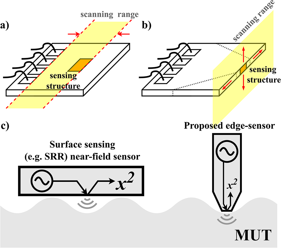
 $\unicode{x03BC}$m must be maintained [Reference Grzyb, Heinemann and Pfeiffer19, Reference Grzyb, Heinemann and Pfeiffer20]. This proximity requirement makes conventional top-surface designs incompatible with nonplanar or microstructured samples, especially when the characteristic dimensions of surface notches or surface features are smaller than the overall chip boundaries. To address these constraints, this paper presents a 547 GHz integrated near-field imaging probe utilizing a passive sensing structure designed to evaluate material permittivity directly from the diced edge of the chip. The probe incorporates a resonant topology composed of two pairs of folded coupled transmission lines. The diced ends of these transmission lines terminate at the chip edge, leaving them exposed to interact directly with the target medium. The underlying sensing mechanism relies on tracking the resonance shifts caused by the dielectric loading of the target material on the fringing electric fields at the exposed stripline boundaries. A conceptual comparison of different imaging modalities – including conventional antenna-based systems, NSOM, top-surface SRR sensing, and the proposed edge-mounted approach – is illustrated in Fig. 1. By migrating the sensing interface from the top surface to the chip edge, the proposed design avoids the mechanical scanning-range boundaries typically imposed by top-surface bonding wires, thereby facilitating unhindered physical access to the target during scanning operations, as shown in Fig. 2(a) and (b). Furthermore, moving the active sensing region to the chip edge significantly reduces the effective area of the sensing interface. With precise dicing controls, as indicated by the dashed reference line in Fig. 2(b), this methodology improves mechanical compatibility with nonplanar, microstructured surfaces, as conceptually demonstrated in Fig. 2(c). The integrated sensor is fabricated using a 130 nm SiGe Heterojunction bipolar transistor (HBT) technology featuring
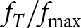 $f_T/f_\mathrm{max}$ figures of 350/450 GHz [Reference Rücker, Heinemann and Fox25]. This manuscript expands upon preliminary results originally presented at the European Microwave Conference (EuMW 2025) [Reference Xinpeng, Andree, Grzyb, Rücker and Pfeiffer26], introducing comprehensive equivalent lumped-element circuit modeling, spatial electric field boundary analysis, and expanded parametric design evaluations. Furthermore, a new measurement verification is included where the relative permittivity of a silicon wafer is estimated by combining simulation results with calibration measurements against air and a metallic target. This estimation is independently validated using a frequency-domain THz spectroscopy system.
Sensing freedom of two near-field sensing mechanisms with wire bonds: (a) top-surface sensing and (b) the proposed edge-sensing approach. (c) Potential operation as a sensing tip with a reduced sensing-part footprint at the chip edge enabled by controlled dicing.

Figure 2 Long description
Three parts illustrate different near-field sensing mechanisms. In the first part, labeled a, a top-surface sensing structure is shown with a scanning range indicated by dashed lines and arrows. The sensing structure is positioned on the surface of a chip, with wire bonds visible. In the second part, labeled b, the proposed edge-sensing approach is depicted. The sensing structure is located at the edge of the chip, with a scanning range marked by dashed lines and arrows, allowing interaction with the target medium. The third part, labeled c, compares surface sensing and the proposed edge-sensor. On the left, a surface sensing mechanism, such as a split-ring resonator near-field sensor, is shown interacting with a material under test, represented by waves emanating from the sensor. On the right, the proposed edge-sensor is illustrated, interacting with the material under test, with waves depicted below the sensor. The edge-sensor is positioned at the chip edge, highlighting its reduced footprint and direct interaction with the target medium.
Sensing concept and circuit design
Figure 3(a) presents the block diagram of the proposed sensing concept. A 0.547 THz triple-push Colpitts oscillator serves as the signal source, providing a relatively stable-frequency signal (varying within  $\pm$ 0.2 GHz) to the input of the sensing structure under a fixed bias, despite changes in the permittivity of the sensing material. The sensing element employs a two-port resonator, comprising two pairs of folded coupled transmission lines, whose diced ends are exposed at the chip edge to interact directly with the sensing target. Its resonant frequency varies monotonically with the permittivity of the object under test (see “Sensing structure” section for details). This frequency shift modulates the power transmitted from the sensor to the detector, as illustrated in Fig. 3(b). The on-chip power detector converts the received power into a DC voltage that also varies monotonically with the input power. Together, these components establish a monotonic mapping between the object’s permittivity and the sensor’s DC output voltage.
(a) Block diagram of the near-field sensing probe. (b) Sensor operation principle. Source: Reproduced from [Reference Xinpeng, Andree, Grzyb, Rücker and Pfeiffer26], Figure 2.

Figure 3 Long description
A block diagram with a source symbol feeding an oscillator labeled, Oscillator with f subscript osc. A vertical block labeled, Sensing Structure, is connected to the oscillator. Next to the sensing structure are two listed cases: I. Vacuum with epsilon subscript r equals 1 and II. Object with epsilon subscript r greater than 1. Below, a detector block is labeled, Detector, with X superscript 2 leading to an arrow labeled, delta V. To the right is the text, DC response. The image B showing a line graph with the y-axis labeled, Power Transmittance and the x-axis labeled, Frequency. Three curves are shown with a legend: vacuum with epsilon subscript r equals 1, with object and with PEC object with epsilon subscript r equals infinity. Each curve forms a dip at a different frequency. A vertical marker at the lowest point of the vacuum curve is labeled, f subscript osc. A horizontal double arrow between two vertical markers near the dip region is labeled, delta f subscript res with resonance frequency. A bracketed annotation to the right of the dip region is labeled, Modulation depth delta Power.
THz source and power detector
The simplified schematic of the complete system is shown in Fig. 4. The on-chip THz source is realized using a previously proposed triple-push Colpitts oscillator in a common-collector topology [Reference Grzyb, Heinemann and Pfeiffer20], which leverages an enhanced third harmonic to achieve an operating frequency ( ${f_\mathrm{osc}}$) beyond the device’s
 ${f_\mathrm{max}}$. In this configuration, a traveling-wave mode introduces progressive phase shifts of 120
 $^{\circ}$ and 240
 $^{\circ}$ between the three Colpitts branches at the fundamental (
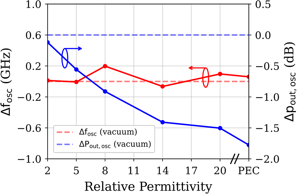
 ${f_\mathrm{osc}/3}$) and the second-harmonic frequencies, respectively. Consequently, the fundamental and second-harmonic components from the three branches cancel at the common-base output node, while the third harmonic constructively superimposes, producing the desired THz output. This arrangement also establishes a virtual AC ground for the fundamental and second-harmonic signals at the push output, minimizing frequency pulling caused by variations in the resonator impedance when loaded with different objects. Figure 5 shows the simulated oscillation frequency shift and output power variation of the oscillator with respect to the sensing target’s permittivity, compared to the no-object case. For different permittivity values of the sensing object, the simulated oscillation frequency varies within a
 $\pm$0.2 GHz range due to changes in the load impedance introduced by different sensing objects. In addition, the simulated delivered output power of the oscillator decreases by approximately 2 dB as the permittivity of the sensing object increases from unity (vacuum) to infinity, where a perfect electric conductor (PEC) is modeled as having infinite permittivity. To preserve the monotonic behavior of the sensor response, the power transmission of the sensing structure at the sensing frequency must also decrease monotonically with permittivity.
Simplified schematic of the proposed near-field edge sensing probe. Source: Reproduced from [Reference Xinpeng, Andree, Grzyb, Rücker and Pfeiffer26], Figure 3.

Figure 4 Long description
The circuit is divided into three main sections: base bias, sensing structure and power detector. The base bias section includes a resistor labeled R, a capacitor labeled C subscript dc and a transistor labeled T subscript 4, connected to a transmission line labeled TL subscript choke. The sensing structure is depicted with an antenna symbol. The power detector section includes a transistor labeled T subscript 5, a resistor labeled R subscript ext and capacitors labeled C subscript dc and C subscript de, with output voltage labeled V subscript out. Below, the 3-push oscillator section includes three transistors labeled T subscript 1, T subscript 2 and T subscript 3, each connected to capacitors labeled C subscript dc and C subscript e and transmission lines labeled TL subscript a, TL subscript b and TL subscript c. The transmission lines are marked with phase shifts of 0 degrees, 120 degrees and 240 degrees. Additional text indicates TL subscript b: 107 degrees, TL subscript c: 35 degrees, TL subscript choke at f subscript osc over 3, C subscript e: 6.5 femtofarads and R: 250 ohms.
The simulated oscillation frequency shift and output power variation of the oscillator under different sensing target permittivity values, compared with the no-object case (vacuum condition).

The Colpitts oscillator cell employs a transistor with dimensions of  $5\times0$.13
 $\unicode{x03BC}$m
 $\times$0.96
 $\unicode{x03BC}$m. The fundamental oscillation frequency is determined by the transmission line
 $TL_b$, capacitor
 $C_e$, and the capacitance of the base-emitter junction. Frequency tuning is achieved by adjusting the base-emitter capacitance via the base bias, which is itself adjusted via the supply voltage
 $V_{cc}$ using a current mirror. To enhance the third-harmonic output, the termination of the transmission line
 $TL_c$ on the collector node is additionally employed [Reference Pfeiffer, Zhao, Grzyb, Hadi, Sarmah, Förster, Rücker and Heinemann27]. The transmission line at the emitter node
 $TL_e$ provides a DC path while blocking the fundamental AC current, and the capacitor
 $C_{dc}$ ensures decoupling. To shield the oscillator and the power detector on the chip from external interference, both components are buried beneath a grounded top-metal layer (TM2). Figure 6 shows the 3D view of the triple-push Colpitts oscillator, with a partial TM2 cover removed to reveal structural details. The oscillator demonstrates a measured tuning range of 534–563 GHz with a
 ${V_{cc}}$ bias from 2.4 to 1.1 V, an output power of 35
 $\unicode{x03BC}$W, and a DC-to-RF efficiency of 0.038%. For further details on the design approach, see [Reference Pfeiffer, Zhao, Grzyb, Hadi, Sarmah, Förster, Rücker and Heinemann27].
Simplified 3D view of the triple-push Colpitts oscillator, with part of the TM2 cover removed to reveal the structural details of one of the three Colpitts oscillators.

Figure 6 Long description
A simplified 3D view of a triple-push Colpitts oscillator is presented, highlighting structural details with part of the cover removed. Three oscillator sections are labeled as OSC1, OSC2 and OSC3, positioned from bottom left to top right. Transmission lines are marked as TLc and TLe, with TLc located near the top right and TLe extending from the bottom left. Capacitors are labeled as Cdc and Ce, with Cdc positioned at the bottom and Ce near the center. The output is marked as Pout, located at the top right. The layout shows the interconnections between these components, illustrating the arrangement and flow within the oscillator system.
The power detector is realized using a single-cell transistor of dimensions 0.13  $\unicode{x03BC}$m
 $\times$0.96
 $\unicode{x03BC}$m in a common-emitter (CE) configuration. By noncoherently downconverting the input RF power, it produces a DC output signal at the collector node that is proportional to the received power [Reference Andree, Grzyb, Jain, Heinemann and Pfeiffer28]. A bypass capacitor (
 $C_{dc}$) at the collector node establishes an AC ground, while the down-converted DC current generates a voltage drop across an external 17 k
 $\Omega$ resistor (
 $R_{ext}$), see Fig. 4. Based on previous investigations [Reference Grzyb, Heinemann and Pfeiffer19], the detector was biased with a base-emitter voltage (
 $V_{BE}$) of 0.81–0.83 V and a collector-emitter voltage (
 $V_{CE}$) of 0.8–0.9 V, resulting in a maximum current response of 0.48 A/W.
Sensing structure
The edge-sensing structure is realized using the two top thick-metal layers of the back-end-of-line (BEOL) stack-up (see Fig. 7). The sensing element is a resonator composed of two pairs of folded, inter-coupled transmission lines. Capacitive coupling at the ends of these transmission lines generates fringing electric fields at the structure’s edges, as illustrated in the simplified lumped transmission line model in Fig. 7. The interaction between the fringing electric field and materials of different permittivity modifies the capacitive coupling, thereby shifting the resonant frequency of the sensing structure.
A simplified representation of the 3D sensor structure, the sensing object, the corresponding coupled transmission line model of the sensing part, and the simplified BEOL stack-up illustration.

Figure 7 Long description
A 3D sensor structure with various labeled components. At the top left, an input from an oscillator is directed towards a ground labeled GND on layer TM2. The output is directed to a power detector. The structure includes multiple layers with specified thicknesses in micrometers: TM2 at 4, TopVia2 at 2.8, TM1 at 2, TopVia1 at 0.85, M5 at 0.49, Via4 at 0.54, M4 at 0.49, Via3 at 0.54, M3 at 0.49, Via2 at 0.54, M2 at 0.49 and M1 at 0.42. The layers are shown in a vertical stack with an air gap above. A sensing object is positioned adjacent to the structure, interacting with a fringing field. The inset at the bottom right shows a simplified circuit model with capacitive elements and a fringing field symbol, labeled epsilon subscript r. Dimensions are provided: L subscript 1 equals 46 micrometers, L subscript 2 equals 77 micrometers, D subscript 1 equals 8 micrometers and W subscript 1 equals 2 micrometers.
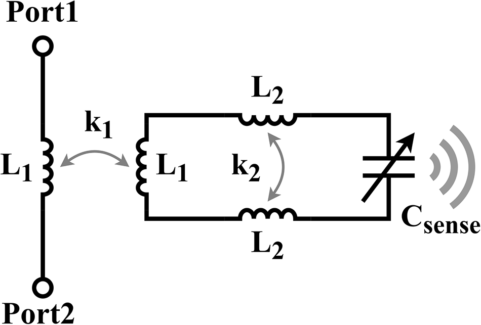
To provide an intuitive understanding of the sensor’s operation, a simplified equivalent lumped-element circuit schematic of the sensing structure is illustrated in Fig. 8. Although the folded coupled transmission lines exhibit highly distributed characteristics at the 547 GHz operating frequency, the qualitative behavior of the system can be modeled as a two-port network utilizing lumped components. The network comprises three primary components: a coupling section interacting with the main path between the oscillator source and detector, a long main coupled sensing stripline, and the exposed sensing ends at the chip edge. For the first two coupled sections, the electrical behavior is dominated by the mutual inductances ( $L_1$ and
 $L_2$). Conversely, at the exposed diced ends, interaction with a targeting object perturbs the localized fringing electric fields. Consequently, the exposed tip is modeled as an equivalent variable series capacitance (
 $C_{\text{sense}}$) terminating the coupled lines.
Simplified equivalent lumped-element circuit model of the sensing structure ( $L_1 = 20\,\text{pH}$,
 $L_2 = 50\,\text{pH}$,
 $k_1 = 0.8$,
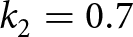 $k_2 = 0.7$,
 $C_{\text{sense}} = 3\,\text{fF}$, and the series resistance of the inductors is
 $R = 1\,\Omega$).

Parametric evaluation of the sensing core design parameters: (a)  $S_{21}$ variations versus frequency with different
 $C_{\text{sense}}$, tuning effects of the sensing stripline (b) length and (c) coupling coefficient on the intrinsic resonance frequency, and (d) spatial boundary where the electric field intensity drops to
 $-30\,\text{dB}$ relative to its peak value at the stripline tip versus the distance between the coupled lines.

Figure 9 Long description
The line graph A has the y-axis labeled, S subscript 2 subscript 1, open parenthesis decibel close parenthesis, ranging from minus 20 to 0. The x-axis is labeled, Frequency, open parenthesis gigahertz close parenthesis, ranging from 250 to 550. A legend lists six curves: C sense equals 2.0 fF, C sense equals 2.5 fF, C sense equals 3.0 fF, C sense equals 3.5 fF, C sense equals 4.0 fF and C sense equals 4.5 fF. Each curve has a single deep minimum between about 300 and 550 gigahertz, with the minimum shifting to higher frequency across the set. The line graph B has the y-axis labeled, S subscript 2 subscript 1, open parenthesis decibel close parenthesis, ranging from minus 20 to 0. The x-axis is labeled, Frequency, open parenthesis gigahertz close parenthesis, ranging from 250 to 550. A legend lists six curves: L subscript 2 equals 30.0 pH, L subscript 2 equals 40.0 pH, L subscript 2 equals 50.0 pH, L subscript 2 equals 60.0 pH, L subscript 2 equals 70.0 pH and L subscript 2 equals 80.0 pH. Each curve has one deep minimum between about 300 and 550 gigahertz, with the minimum shifting across the frequency range across the set. The line graph C has the y-axis labeled, S subscript 2 subscript 1, open parenthesis decibel close parenthesis, ranging from minus 20 to 0. The x-axis is labeled, Frequency, open parenthesis gigahertz close parenthesis, ranging from 250 to 550. A legend lists six curves: k subscript 0 equals 0.6, k subscript 0 equals 0.65, k subscript 0 equals 0.7, k subscript 0 equals 0.75, k subscript 0 equals 0.8 and k subscript 0 equals 0.85. Each curve has one deep minimum between about 300 and 550 gigahertz, with the minimum shifting across the frequency range across the set. The line graph D has the y-axis labeled, minus 30 decibel boundary, open parenthesis micrometer close parenthesis, ranging from 15.0 to 25.0. The x-axis is labeled, Distance, open parenthesis micrometer close parenthesis, ranging from 4 to 16. The plotted line has four marked points at distance 4 with about 16.0, distance 8 with about 21.5, distance 12 with about 23.0 and distance 16 with about 19.0.
To illustrate how these core design parameters influence the overall sensor performance, Fig. 9 presents a series of parametric evaluations. It is worth noting that the component values implemented in this lumped circuit model are selected purely as illustrative examples to demonstrate qualitative trends and underlying sensing behaviors, rather than representing extracted parameters from the actual circuit. As shown in Fig. 9(a), variations in the object’s relative permittivity directly alter  $C_{\text{sense}}$, which shifts the resonance frequency of the sensing structure. Because the source oscillator operates at a fixed frequency, this resonance shift alters the transmitted power through the network, meaning the power delivered to the detector becomes a direct function of the target material’s permittivity. The intrinsic resonant frequency of the sensing structure is primarily determined by the physical length and the coupling coefficient of the sensing stripline, as shown in Fig. 9(b) and (c), respectively. The physical length can be further retuned during the post-dicing process before measurement, whereas the coupling coefficient is primarily controlled by the lateral spacing between the coupled lines. In addition to governing the coupling coefficient, this line spacing also influences the spatial distribution of the electric field at the exposed ends of the diced chip. Figure 9(d) maps the spatial boundary where the electric field intensity drops to
 $-30\,\text{dB}$ relative to its peak value at the stripline tip. A narrower spacing between the coupled lines provides a higher coupling coefficient but results in a highly constrained electric field profile. This localized field distribution provides superior lateral spatial resolution, but the field intensity decays faster with distance. Conversely, increasing the line spacing within a certain range allows the fringing electric field to spread further outward from the sensing tip. This expanded field profile enhances the maximum detectable distance, albeit at the cost of lower lateral resolution. Therefore, the line spacing serves as a critical design degree of freedom to balance resolution against sensing range. The finalized design parameters are implemented as shown in the 3D layout.
To enable edge sensing, the chip is diced perpendicular to the transmission lines, exposing their cross-section to air. In simulations, an air gap of approximately 0.5  $\unicode{x03BC}$m is maintained between the sensor and the object to account for irregularities on the diced edge and to ensure smooth scanning. The measurement results indicate that approximately 72% of the sensor response is retained at a distance of 0.5
 $\unicode{x03BC}$m (see “Sensor characterization” section).
Simulated frequency dependence of power transmitted through the sensing structure for objects with different  $\varepsilon_{r}$ and PEC.

Figure 10 Long description
Power Transmission The x-axis label is, Frequency (GHz). The x-axis ranges from 400 to 700, with labeled ticks at 400, 450, 500, 550, 600, 650 and 700. The y-axis label is, Power Transmission. The y-axis ranges from 0.0 to 1.0, with labeled ticks at 0.0, 0.2, 0.4, 0.6, 0.8 and 1.0. A legend lists seven curves: No object, epsilon subscript r equals 2, epsilon subscript r equals 5, epsilon subscript r equals 8, epsilon subscript r equals 14, epsilon subscript r equals 20 and PEC. All curves start near 0.8 to 0.9 at 400 gigahertz, then drop to a minimum near the middle of the plot and then rise again toward 700 gigahertz. The minima occur at different frequencies for different curves. The curve labeled No object has its minimum near about 600 gigahertz. The curve labeled PEC has its minimum near about 560 gigahertz. The other epsilon subscript r curves have minima between these two frequencies, ordered progressively from higher frequency toward lower frequency as epsilon subscript r increases. A vertical arrow annotation near the dip is labeled, Modulation depth at sensing freq. Three text regions appear along the top: Monotonically decrease versus epsilon subscript r on the left, Non monotonically on the middle and Monotonically increase versus epsilon subscript r on the right.
The 3D electromagnetic simulation performed in Ansys HFSS reveals the frequency-dependent power transmission from the oscillator to the detector for objects with varying relative permittivity ( $\varepsilon_{r}$), as shown in Fig. 10. The sensing structure’s resonant frequency decreases monotonically from 625 to 565 GHz as the permittivity of the object increases, starting from the vacuum (
 $\varepsilon_{r}=1$) and reaching its maximum shift for a PEC (
 $\varepsilon_{r}=\infty$).
For operating frequencies above the resonance of the objectless sensor or below that of the sensing structure with the PEC object, the power transfer coefficient varies monotonically with the permittivity of the sensed object, corresponding to the two monotonic regions marked in Fig. 10. As discussed in “THz source and power detector” section and illustrated in Fig. 5, the delivered output power of the oscillator decreases with increasing permittivity of the sensing object. To ensure an overall monotonic sensor response, the power transmission of the sensing structure at the sensing frequency must also decrease monotonically with permittivity. Therefore, the left monotonic region of the sensing structure shown in Fig. 10 is selected for the sensing operation.
The difference in transmitted power at a given frequency between the vacuum and PEC cases defines the mapping range across all permittivity values, representing the modulation depth at that frequency. A larger modulation depth corresponds to a greater power transfer difference between two closely spaced permittivity values, thereby providing higher sensing sensitivity. To avoid non-monotonic operation caused by discrepancies between simulation and measurement, the operating frequency is selected with sufficient margin from the boundary of the left monotonic region, as shown in Fig. 10. Based on simulation results, a sensing frequency of 547 GHz ( $V_{cc}$=1.6 V) is selected to achieve a relatively high modulation depth while providing sufficient margin to accommodate potential frequency shifts between simulation and practical operation. The total resonance shift of approximately 60 GHz limits the modulation depth, which is determined by the position of the power transmission curve within its monotonic operating region, and optimizing this parameter represents a direction for future research.
(a) Top view and (b) side view of the electric-field distribution in the sensing structure.

Figure 11 Long description
A heatmap labeled, Top View, of E field [V/m]. The color scale is labeled, E field [V/m], with Max: 3.304E plus 06 and Min: 4.556E plus 03. Text inside the map reads, E field intensity slash max. value. A rectangular conductor feature is labeled, TM2 sensing strip line. A right pointing arrow starts at the strip edge. Along the arrow, the labels read, 20 percent, 35 micro m and 1 percent. The image B showing a heatmap labeled, Side View, of E field [V/m]. The color scale is labeled, E field [V/m], with Max: 3.304E plus 06 and Min: 4.556E plus 03. Three stacked rectangular layers are labeled, TM2 sensing strip line, M2 ground plane and TM1 sensing strip line.
Figure 11 shows the electric-field distribution surrounding the sensing structure at the sensing frequency of 547 GHz. The field amplitudes are calculated for a 1 W reference excitation power. The electric-field strength at the edge of the sensing structure decreases rapidly with distance. In a vacuum, the field strength at a distance of 5  $\unicode{x03BC}$m from the edge drops to approximately 20% of its maximum value at the edge of the sensing structure, and further decreases to about 1% at a distance of 35
 $\unicode{x03BC}$m.
Measurement
The micrograph of the diced chip and the exposed cross-section of the sensing structure are shown in Fig. 12. The diced chip has dimensions of 300  $\unicode{x03BC}$m
 $\times$ 445
 $\unicode{x03BC}$m. For sensor characterization, a metallic cutter blade is first employed to evaluate the sensing range and lateral resolution at an operating frequency of 547 GHz. Subsequently, a slice of float-zone silicon (FZ-Si) wafer was used as the sensing target. Based on the measured sensor responses for the air and a metallic target, together with simulated results, the relative permittivity of the wafer is estimated. To verify this estimation, an independent measurement of the wafer’s relative permittivity was performed using a Toptica continuous-wave (CW) frequency-domain THz spectroscopy system. Finally, a motorized translation stage is used to perform two-dimensional raster scanning of the metal cutter blade, demonstrating the imaging capability of the proposed sensor.
Micrograph of a diced chip and cross-section of the sensing structure.

Figure 12 Long description
An annotated die micrograph of a chip with dimensions labeled as 300 micrometers by 445 micrometers. It features a triple-push oscillator centrally located, with visible connections to capacitors and inductors. The oscillator is linked to a power detector, which is positioned to the right. The chip surface includes transmission lines and bond pads, indicating the circuitry layout. An inset in the top right corner shows a magnified cross-section of the sensing structure, labeled ′Sensing Structure′ and ′Cross-Section,′ highlighting the internal design of the sensor. The diagram illustrates the integration of the triple-push oscillator with the power detector and sensing structure, demonstrating the chip′s functionality and design. The inset provides detailed insight into the sensor′s construction, emphasizing its role in the system.
Sensor characterization
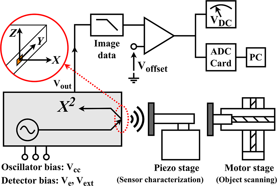
The simplified block diagram of the sensor measurement setup is shown in Fig. 13. The device is biased using a low-noise power supply (Keysight B2962A) in combination with low-pass filters (Keysight N1294A opt. 020). Based on the simulated results shown in Fig. 10, the sensor exhibits its maximum response to a PEC object at the sensing frequency of 547 GHz. Therefore, a metallic cutter blade is used as the sensing object to evaluate the maximum sensing range. The position sweep coordinate system is illustrated in Fig. 13.
Block diagram of the measurement setup, a three-axis piezoelectric stage is used for the sensor characterization, while a motorized translation stage is employed for 2D raster-scanning of the object.

Figure 13 Long description
The sensor measurement setup features several components. At the top left, a coordinate system labeled Z, Y, X is shown within a red circle, indicating the position sweep. Below this, an oscillator bias labeled V subscript oc and a detector bias labeled V subscript dc minus V subscript st are connected to a box marked X superscript 2. This box is linked to a piezo stage labeled sensor characterization and a motor stage labeled object scanning. The piezo stage is positioned to the right of the X superscript 2 box, while the motor stage is further to the right. Above the X superscript 2 box, an arrow labeled V subscript out points towards an image data box, which is connected to an amplifier labeled V subscript offset. This amplifier is linked to an ADC card, which is connected to a PC. The setup is designed to process image data from the sensor, with the piezo stage used for sensor characterization and the motor stage employed for object scanning.
From the simulated electric-field distribution shown in Fig. 11(a), the sensing range is estimated to be on the order of tens of micrometers. Similarly, the lateral resolution is primarily determined by the physical dimensions of the sensing structure and the scale is also on the order of tens of micrometer. To achieve accurate characterization, a three-axis piezoelectric stage (MAX312D) driven by a piezo controller (MDT693B) from Thorlabs is employed for object scanning, together with a digital multimeter (Keysight 34460A) for signal readout. For the metal cutter blade sweep used in the sensor characterization, when the object is sufficiently far from the sensor, it has no impact on the electric field distribution, which is equivalent to a vacuum environment. When the object reaches the minimum sweep distance, the configuration corresponds to a PEC boundary condition. Therefore, the intermediate positions during the distance sweep are equivalent to an object with an effective relative permittivity ranging from 1 to infinity. As a result, the maximum operating frequency variation across the entire distance sweep remains inherently limited to  $\pm$0.2 GHz, as shown in Fig. 5.
(a) Measured sensor response decay rate for a metallic object as a function of the sensor-to-object distance. Measured sensor lateral resolution for a metallic object along (b) the y- and (c) z-axis directions of multiple measurements at 547 GHz.

Figure 14 Long description
A line graph with the vertical axis label, Normalized Sensor Response and tick labels 0.0, 0.2, 0.4, 0.6, 0.8, 1.0. The horizontal axis label is, X-Axis Distance (micro-meter), with tick labels 0, 2, 4, 6, 8, 10, 12, 14, 16, 18, 20. A legend lists Trial 1, Trial 2, Trial 3. An annotation reads, Max. sensing range: 19 micro-meter. Three curves start near 1.0 at 0 micro-meter and drop steeply by about 2 micro-meter, then continue decreasing gradually toward values near 0.0 by 20 micro-meter. The image B showing a line graph with the vertical axis label, Normalized Sensor Response and tick labels 0.0, 0.2, 0.4, 0.6, 0.8, 1.0. The horizontal axis label is, Y-Direction Travel Distance (micro-meter), with tick labels 2, 4, 6, 8, 10, 12, 14, 16, 18, 20. A legend lists Trial 1, Trial 2, Trial 3. Two horizontal reference lines are labeled, 90 percent Response and, 10 percent Response. An annotation reads, Y-resolution: 11.8 micro-meter. The three curves begin near 1.0 at about 2 micro-meter, decrease with distance, cross below 0.2 between about 14 micro-meter and 16 micro-meter and approach values near 0.0 by 20 micro-meter. The image C showing a line graph with the vertical axis label, Normalized Sensor Response and tick labels 0.0, 0.2, 0.4, 0.6, 0.8, 1.0. The horizontal axis label is, Z-Direction Travel Distance (micro-meter), with tick labels 2, 4, 6, 8, 10, 12, 14, 16, 18, 20. A legend lists Trial 1, Trial 2, Trial 3. Two horizontal reference lines are labeled, 90 percent Response and, 10 percent Response. An annotation reads, Z-resolution: 7 micro-meter. The three curves begin near 1.0 at about 2 micro-meter, decrease with distance, cross below 0.2 between about 8 micro-meter and 12 micro-meter and approach values near 0.0 by 20 micro-meter.
Figure 14(a) presents the measured decay of sensor response as a function of the object’s distance from the chip diced edge along the x-axis. Three scanning trials are conducted during sensor characterization to verify repeatability. The maximum detectable distance is defined by the noise floor of the measurement system, representing the point where the change in the normalized sensor response falls below the system noise level. This corresponds to a signal-to-noise ratio (SNR) approaching unity, beyond which the sensor response can no longer be reliably distinguished from background noise. Based on this criterion, the maximum detectable distance for a metallic object is determined to be approximately 19  $\unicode{x03BC}$m.
For the characterization of the sensor’s lateral resolution, the commonly used 10–90% rising/falling edge criterion [Reference Grzyb, Heinemann and Pfeiffer19] is adopted. To ensure smooth scanning despite unevenness of the surface introduced by the dicing, an approximate 0.5  $\unicode{x03BC}$m gap is maintained between the chip edge and the object during movement along the y- and z-axis directions. Since the sensor response decreases rapidly with increasing distance, as indicated in Fig. 14(a), the metallic cutter blade is still used as a sensing object to ensure a sufficiently strong and clearly detectable response for lateral-resolution evaluation. The blade is moved along the y- and z-axis directions, respectively, while ensuring that the regions of both stable maximum and minimum response are captured to extract the 10–90% rising and falling edges. The measured sensor responses along the y- and z-axis directions are shown in Fig. 14(b) and (c). The extracted horizontal and vertical resolutions are 12 and 7
 $\unicode{x03BC}$m, respectively, corresponding to values smaller than
 $\lambda$/45 at the sensing frequency of 547 GHz, thus demonstrating super-resolution performance.
Permittivity measurements
When the distance between the sensing object and the sensor is fixed, the sensor response varies monotonically with the target material’s permittivity, as discussed in “Sensing structure” section. This characteristic enables the sensor to function as a permittivity meter for material characterization. In this study, a slice of FZ-Si wafer is used as the sensing target. In this study, a slice of FZ-Si wafer is used as the sensing target to validate the sensor performance through contact measurements. This specific material was selected based on its mechanical and electrical properties. Mechanically, the wafer is solid and flat, which is necessary to satisfy the strict alignment and contact requirements of the implemented edge sensing strategy. Electrically, the operating principle of the proposed sensor primarily accounts for the real part of the relative permittivity. Because FZ-Si is well-characterized up to several THz and exhibits a negligibly small imaginary part (dielectric loss) as reported in [Reference Dai, Zhang, Zhang and Grischkowsky29], it serves as an ideal reference material to verify the sensor response.
For permittivity extraction, simulated sensor voltage responses  $V_{sim,i}$ corresponding to sensing objects with different relative permittivity values
 $\epsilon_r=i$ are first obtained. Two reference cases are considered in simulation: a vacuum object and a PEC object, yielding
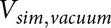 $V_{sim,vacuum}$ and
 $V_{sim.PEC}$, respectively. Using these reference values, the simulated responses are normalized to obtain the normalized simulated sensor responses
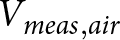
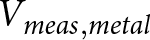
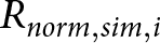 $R_{norm,sim,i}$, which are then used to construct a normalized sensor-response interpolation function. In the measurement, the sensor voltage response obtained with a FZ-Si wafer as the sensing object is denoted as
 $V_{meas,wafer}$. Likewise, two experimental reference cases, air and a metallic object, are measured, resulting in
 $V_{meas,air}$ and
 $V_{meas,metal}$, respectively. The measured wafer response is normalized using these reference values in the same manner as in the simulation. The normalized measured response of the wafer
 $R_{nrom,meas}$ is then mapped onto this function to determine the corresponding permittivity value.
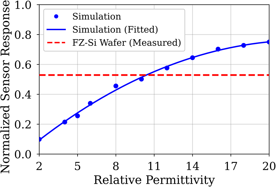
Simulated sensor response of sensing objects with different permittivity normalized with vacuum and PEC objects, and measured sensor response of an FZ-Si wafer slice normalized with air and a metallic object.

This normalization procedure compensates for offset and gain discrepancies between simulation and measurement, reduces the influence of absolute voltage scaling errors, and mitigates measurement drift. Consequently, the normalized simulated and measured responses become directly comparable, enabling the permittivity extraction. The normalization procedure is defined by equations 1 and 2. The normalized simulated sensor response as a function of relative permittivity, together with the normalized measured sensor response of the FZ-Si wafer, is shown in Fig. 15. From this comparison, the corresponding relative permittivity of the wafer is estimated to be 10.21.
 \begin{equation}
R_{norm,sim,i}=\frac{V_{sim,i}-V_{sim,vacuum}}{V_{sim,PEC}-V_{sim,vacuum}}
\end{equation}
 \begin{equation}
R_{norm,meas}=\frac{V_{meas,wafer}-V_{meas,air}}{V_{meas,metal}-V_{meas,air}}
\end{equation}
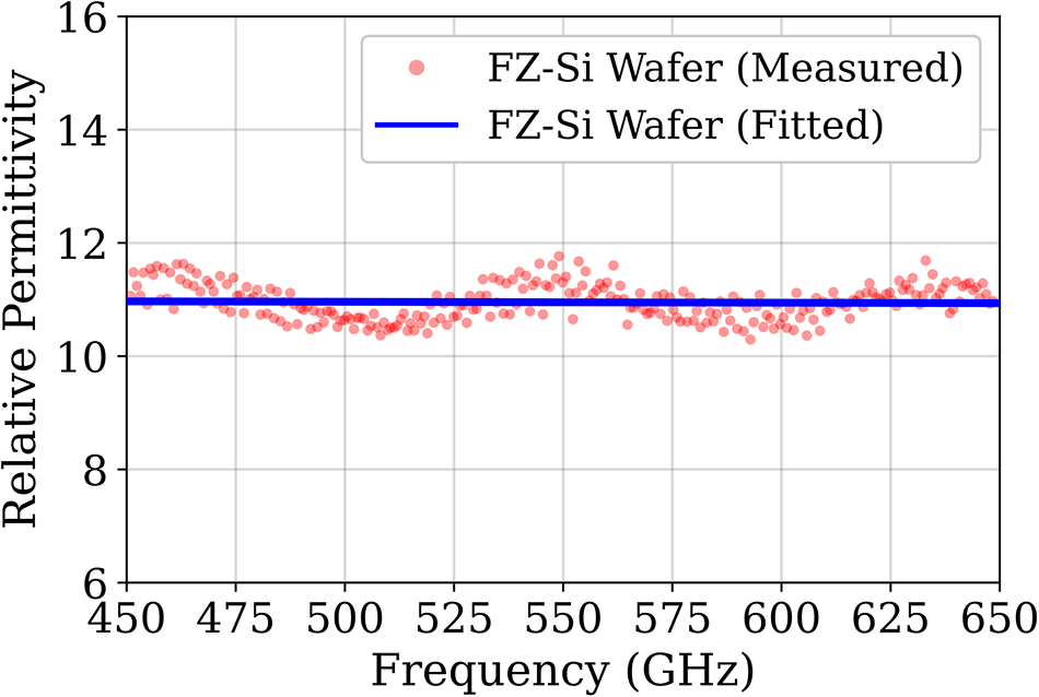
To validate the permittivity estimation, an independent measurement is performed over 450–650 GHz frequency range using a Toptica CW frequency-domain THz spectroscopy system with a 1550-nm laser source, and the measurement setup is illustrated in Fig. 16. In this system, the THz signal is generated by down-conversion of two optical laser tones. The resulting mixed photocurrent signals at the transmitter (Tx) and receiver (Rx) contain both phase and amplitude information. The permittivity is extracted from the relationship between the photocurrent signal measured with the material under test and the reference medium, typically air. The measured relative permittivity and its fitted curve obtained from the THz spectroscopy system are shown in Fig. 17.
Permittivity measurement setup of a 0.5 mm thick FZ-wafer with the Toptica CW frequency-domain THz spectroscopy system with a 1550-nm laser source.

Permittivity measurement result with the Toptica CW frequency-domain THz spectroscopy system of the FZ-Si wafer and fitting curve versus frequency.

At the sensing frequency of 547 GHz, the extracted relative permittivity is 10.95. The deviation between the sensor-based estimation and the THz spectroscopy system measurement is approximately 6.76%. These results are also consistent with previously reported values in [Reference Dai, Zhang, Zhang and Grischkowsky29], Additionally, based on the simulation results in Fig. 15, the normalized sensor response varies non-linearly with the object’s relative permittivity. The rate of change is rapid at lower permittivity values and gradually decreases as the permittivity increases. Specifically, the lower relative permittivity range from  $\varepsilon_r = 1$ to 20 occupies 75% of the total sensor response range, whereas the remaining range from 20 to infinity (PEC) accounts for 25%. Consequently, within this lower permittivity range, the sensor response exhibits higher sensitivity and increased linearity. Taken together, these findings demonstrate the permittivity estimation capability of the proposed sensor.
2D raster-scanning
2D raster-scanning measurement setup of a metallic cutter blade.

2D raster-scanned image of a metallic cutter blade with main scan parameters: size: 500  $\times$ 280
 $\unicode{x03BC}$m
 $^2$, equivalent y-step: 10 nm, z-step: 9.375 nm, ADC sampling rate: 2 kHz, operation frequency: 547 GHz, and distance between sensor and cutter blade:
 $\sim$0.5
 $\unicode{x03BC}$m.

Figure 19 Long description
The plot has a horizontal axis labeled, Y Direction (micrometer), with tick labels at 0, 100, 200, 300, 400 and 500. The vertical axis is labeled, Z Direction (micrometer), with tick labels at minus 200, minus 100, 0, 100 and 200. A vertical color scale at the right is labeled, Amplitude (millivolt), with tick labels at 0, 50, 100, 150 and 200. The main heatmap shows a mostly uniform field with one narrow vertical band of higher amplitude located slightly right of the 200 micrometer tick and left of the 300 micrometer tick, extending from the bottom to the top of the plotted Z range. An inset at the upper left contains a small grayscale image with a red arrow and a short red text label that is not fully legible. A second inset below it shows a line plot with a horizontal axis labeled in micrometer and a vertical axis labeled in millivolt. The line plot contains a single sharp peak near the middle of the horizontal range, with the curve near the baseline elsewhere.
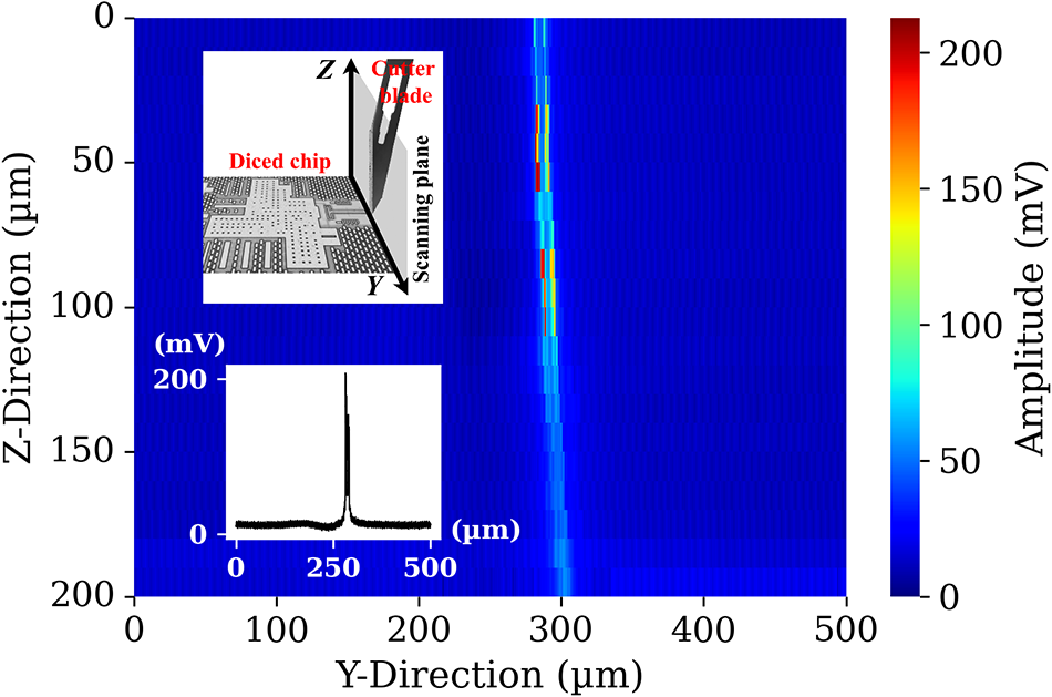
To assess the imaging capability of the proposed sensor, the limited travel range of the piezoelectric stage (20  $\unicode{x03BC}$m) requires the use of two linear translation stages (OWIS GmbH) to enable a millimeter-range 2D raster scanning. An ADC card (NI USB-6210) is employed to achieve a kHz-level sampling rate. A metallic cutter blade is used as the imaging object, and an approximate 0.5
 $\unicode{x03BC}$m gap is maintained between the chip edge and the cutter blade to ensure smooth scanning despite surface unevenness introduced by dicing, and the photograph of the measurement setup is presented in Fig. 18. The resulting 2D raster-scanned image of the cutter blade is shown in Fig. 19, obtained with an ADC sampling rate of 2 kHz. An equivalent step size of 10 nm in the y-direction is achieved by adjusting the motor speed. During object scanning, an SNR of 28.5 dB is observed.
Comparison of state-of-the-art terahertz super-resolution imaging devices

Table 1 Long description
Columns list technology, resolution in micrometers, super resolution level in lambda, frequency in terahertz, PDC in milliwatts, SNR in decibels, integration level, pixel number, sensing structure location, and reference. NSOM reports resolution from 0.035 to 359 micrometers, super resolution level from 1 over 3172 to 1 over 2, frequency from 0.2 to 8.5 terahertz, all external integration, 1 pixel, and external detector, with PDC and SNR not given. Confocal waveguide reports 1410 micrometer resolution at 0.1 terahertz with super resolution level 1 over 2, all external integration, 1 pixel, and external detector, with PDC and SNR not given. Three 130 nanometer SiGe entries at about 0.533 to 0.562 terahertz list on chip sensor integration, 1 pixel for two rows and 2 by 64 pixels for one row, chip top surface sensing, with SNR values of 20 to 40 with marker a, 42 with marker b, and 63.8 with marker c plus 38.5 with marker d, and PDC given as 79 milliwatts only for the 2 by 64 pixel row. 65 nanometer CMOS lists resolution 90 to 160 with marker e at 0.12 terahertz, super resolution level 1 over 14 with marker e, PDC 34.8 milliwatts, on chip sensor integration, 16 by 12 pixels, chip top surface sensing, and no SNR value. 28 nanometer CMOS lists resolution 46 to 54 with marker e at 0.199 to 0.219 terahertz, super resolution level 1 over 16 with marker e, PDC 79 milliwatts, SNR 59.7 with marker f, on chip sensor integration, 10 by 20 pixels, and chip top surface sensing. A 130 nanometer SiGe row at 0.32 terahertz lists two resolution ranges, 13 to 15 with marker g and 50 to 100 with marker e, two super resolution levels, 1 over 61 with marker g and 1 over 9 with marker e, PDC 280 milliwatts, SNR 81.22 with marker h, on chip sensor integration, 32 by 32 pixels, and chip top surface sensing. The row labeled This work lists 130 nanometer SiGe at 0.547 terahertz with 7 to 12 micrometer resolution, super resolution level 1 over 45, PDC 51.6 milliwatts, SNR 28.5 with marker i, on chip sensor integration, 1 pixel, and sensing structure at the chip side edge.
a Estimated from Fig. 24(a) in [Reference Grzyb, Heinemann and Pfeiffer19].
b Estimated from Fig. 19(b) in [Reference Grzyb, Heinemann and Pfeiffer20].
c Dynamic range measured with a lock-in amplifier with 1 ms integration time and 12 dB/oct filter slope (1.17 fps).
d Dynamic range of the digital readout at 28 fps and four averaged samples.
e Pixel size.
f Equivalent noise bandwidth (ENBW) = 100 Hz.
g Resolution of sensing structure.
h Effective number of bits (ENOB) = 13.2 bits from a 14-bit ADC.
i ADC sampling rate of 2 kHz,  $\sim$ 0.5 µm distance between sensor and object.
Conclusion
This paper demonstrates a THz super-resolution near-field imaging probe that senses from the diced chip edge, operating at 547 GHz with a lateral resolution of 7–12  $\unicode{x03BC}$m, corresponding to approximately
 $\lambda$/45 at the sensing frequency, and a maximum responsive distance of 19
 $\unicode{x03BC}$m. Compared with conventional top surface-sensing near-field sensors, particularly those with wire bonds, the proposed edge-sensing architecture offers enhanced sensing flexibility. When operated as a permittivity sensor, measurement performed on a FZ-Si wafer slice exhibit a deviation of 6.76% compared with results obtained using a Toptica CW frequency-domain THz spectroscopy system. These measurement results show good agreement with previously reported values in [Reference Xinpeng, Andree, Grzyb, Rücker and Pfeiffer26]. The SNR of sensing a metallic object is 28.5 dB with a 2 kHz ADC sampling rate and an approximate 0.5
 $\unicode{x03BC}$m separation between the sensor and the object. Table 1 presents a comparison of state-of-the-art THz super-resolution imaging sensors.
Future work could explore higher-precision laser dicing techniques to achieve smoother chip edges. Reduced edge unevenness allows a smaller sensor-object separation during scanning, which, according to simulation, can improve the sensor response by approximately 16% when the distance is decreased from 0.5  $\unicode{x03BC}$m to 0.2
 $\unicode{x03BC}$m, thereby enhancing imaging quality. In addition, the cutting method indicated by the dotted line in Fig. 2(b) can be implemented to adapt the sensor as a sensing tip with a reduced sensing-part footprint at the chip edge. This approach could enable surface-following capability, making the proposed sensor potentially suitable for the characterization of nonplanar microstructures.
Funding statement
The research work presented in this paper was funded by the Ministry of Culture and Science of the State of North Rhine-Westphalia (MKW NRW) through the terahertz. NRW project and the German Research Foundation (DFG) priority program SPP 1857 “ESSENCE” (“Electromagnetic Sensors for Life Sciences”): NearSense.
Competing interests
The authors declare none.

Xinpeng Du received the B.Sc. degree in microelectronics science and engineering from Xidian University, Xi’an, China, in 2018, and the Dipl.-Ing. in electrical engineering in the branch of microelectronics from Technical University of Dresden (TUD), Dresden, Germany, in 2023. He is currently pursuing the Ph.D. degree with the Institute for High Frequency and Communication Technology, University of Wuppertal, Wuppertal, Germany. His main research interest is terahertz integrated circuit and system design in silicon technologies. He is a co-recipient of the 2025 European Microwave Integrated Circuits Conference (EuMIC) Best Paper Prize.

Marcel Andree received the M.Sc. degree and Ph.D. degree (passed with honors) in electrical engineering from the University of Wuppertal, Wuppertal, Germany, in 2017 and 2023, respectively, where he focused on the development and optimization of integrated mixed signal circuits and silicon-integrated circuits for THz imaging applications. Since 2017, he has been a Research Staff Member with the Institute for High-Frequency and Communication Technology (IHCT), Wuppertal. Currently, he is a Group Leader for integrated circuit design at the University of Wuppertal. His research interests include terahertz integrated circuit and system design in silicon technologies. He is a co-recipient of the 2025 European Microwave Integrated Circuits Conference (EuMIC) Best Paper Prize.

Janusz Grzyb received the M.Sc. degree (cum laude) in electronic engineering from the integrated Circuits Laboratory, Gdansk University of Technology, Gdansk, Poland, in 1998, and the Ph.D. degree from the Swiss Federal Institute of Technology, Zurich, Switzerland, in 2004. From 2004 to 2006, he was with the Communication System Design and High-Speed/Optical Packaging Groups, IBM T. J. Watson Research Center, Yorktown Heights, NY, USA. From 2006 to 2009, he was with the Research and Development Group, Huber&Suhner, Pfaffikon ZH, Switzerland. From 2009 to 2024, he was with the Institute for High-Frequency and Communication Technology, University of Wuppertal, Wuppertal, Germany. His research interests include all aspects of silicon-integrated THz electronics.

Holger Rücker received the Diploma and Doctorate degree in physics from the Humboldt University of Berlin, Berlin, Germany, in 1986 and 1988, respectively. From 1989 to 1991, he was a Staff Member with the Humboldt University of Berlin. From 1991 to 1992, he was with the Max Planck Institute for Solid State Research, Stuttgart, Germany. In 1992, he joined IHP, Frankfurt (Oder), Germany, where he is engaged in research on the physics and fabrication of semiconductor devices. He has also led the development of IHP’s 130-nm SiGe BiCMOS technologies SG13S, SG13G2, and SG13G3. His research interests include SiGe bipolar devices, the development of CMOS and BiCMOS technologies, and their application in radio-frequency integrated circuits.

Ullrich R. Pfeiffer received the diploma degree and Ph.D. degree in physics from the University of Heidelberg, Heidelberg, Germany, in 1996 and 1999, respectively. In 1997, he worked as a Research Fellow with the Rutherford Appleton Laboratory, Oxfordshire, England. From 1999 to 2001, he worked as a Postdoctoral Researcher with the University of Heidelberg, and with the European Organization for Nuclear Research (CERN), Geneva, Switzerland. From 2001 to 2006, he was with the IBM T.J. Watson Research Center, Yorktown Heights, NY, USA. Since 2008, he has been holding the High-Frequency and Communication Technology chair at the University of Wuppertal, Wuppertal, Germany. His current research interests include silicon RFICs for mmWave/THz communications, radar, and imaging systems.















 Open access

