NOMENCLATURE
- MOC
method of characteristics π Pi
- γ
ratio of specific heat at constant pressure to specific heat at constant volume
- (x, r)
cylindrical coordinates of axisymmetric basic flow model, m
- (z, y)
rectangular coordinates on base plane of vehicle, m
- ϕ
angle between axial plane and plane of symmetry, °
- δ CG (x)
distribution of angle of slope along wall CG, °
- M CG (x)
distribution of Mach number M along wall CG
- M C
mach number at point C in integrated axisymmetric basic flow model
- θ DC,2 (x)
distribution of flow angle θ just downstream of cowl shock wave DC, °
- x CF
distance in x-direction between points C and F, m
- θ
flow angle, °
- M 0
free-stream Mach number
- M
local Mach number
- Re0
free-stream Reynolds number per unit length, /m
- P 0
free-stream pressure, Pa
- P
local static pressure, Pa
- P/P 0
ratio of local static pressure to free-stream static pressure
- P t,0
free-stream total pressure, Pa
- T 0
free-stream temperature, K
- T
local temperature, K
- T t,0
free-stream total temperature, K
- α
angle-of-attack, °
- β
shock wave angle, °
- C L
lift coefficient
- C D
drag coefficient
- C mz
pitching moment coefficient
- L/D
lift-to-drag ratio
- M e
area-weighted average Mach number at exit of isolator
- P e/P 0
area-weighted average pressure rise ratio at exit of isolator
- T e/T 0
area-weighted average temperature rise ratio at exit of isolator
- P e,t/P 0,t
area-weighted average total pressure recovery at exit of isolator
- ṁ
area-weighted average capture mass flow rate at exit of isolator, kg/s
- σ
area-weighted average capture mass flow coefficient at exit of isolator
1.0 INTRODUCTION
A large number studies conducted since the 1960s have shown that one of the key factors for ensuring the success of an air-breathing hypersonic vehicle is an effective design for the airframe/engine integration(Reference O’Neill1–Reference Ding, Liu, Shen and Huang4). The engine needs to be incorporated as an integral part of the airframe to reduce the drag and achieve a positive thrust. Therefore, the aerodynamics of the airframe and engine become strongly related.
Hypersonic propulsion systems rely mainly on scramjet engines, including inlets, combustion chambers, and nozzles(Reference Heiser and Pratt5). The layout, location, and number of scramjet engines on the airframe of an air-breathing hypersonic vehicle are diverse, and they should be designed according to mission requirements. The inlet needs to provide a compressed air stream for the scramjet combustor, and the airflow that needs to be captured upstream may be disturbed by the various components of the airframe. The combustion chamber and nozzle are usually the internal components, and their upstream flow depends mainly on the performance parameters of the inlet or outlet of the combustion chamber, without having any interfering effect on the flow of the airframe. Hence, one of the core design aspects of airframe/propulsion integration is the design of airframe/inlet integration(Reference Haney and Beaulieu6).
The waverider first proposed by Nonweiler(Reference Nonweiler7) in 1959 is any hypersonic lifting body with an attached shock wave along its leading edge(Reference Liu, Ding, Huang and Jin8–Reference Ding, Liu, Shen, Liu, Chen and Fu14). Since then, because of the excellent aerodynamic configuration of the waverider, it has become one of the most ideal aerodynamic configurations for hypersonic vehicles. There are two advantages of using the waverider concept in the design of an air-breathing hypersonic vehicle(Reference Ding, Liu, Shen and Huang4). First, a waverider can be used as the ideal precompression surface of the inlet because the leading-edge shock wave generated by the waverider can precompress the air and limit leakage of the high-pressure air from the lower surface to the upper surface; the waverider can also capture a considerably greater amount of air. Second, the waverider has a higher lift-to-drag ratio compared with a conventional lifting body at the same lift coefficient, owing to the greater pressure difference between the lower and upper surfaces of the waverider(Reference Lewis15). Thus, a waverider can possess the ideal precompression surface of an inlet system as well as high lift-to-drag ratio characteristics. However, the aerodynamic performance of the waverider with engine integration is expected to become considerably lower than that of the pure waverider. As a result, over the past 60 years, design methodologies for airframe/engine integrated waverider vehicles have been extensively studied by researchers. Problems associated with aerodynamic design method of an airframe/inlet integrated waverider vehicle are addressed, as a first step in the airframe/engine integration.
Two classes of general theories and methods exist for using the waverider concept in the design of air-breathing hypersonic vehicles(Reference O’Neill1,Reference Ding, Liu, Shen and Huang4,Reference Stevens16,Reference Ding, Liu, Shen, Huang, Liu and Chen17) . In the first class of methodologies, the waverider is used only as the vehicle’s forebody, and it behaves as the precompression surface to efficiently provide the inlet with the required compression flow fields; therefore, this class of methodologies is termed the waverider forebody/inlet integration design methodology. In the second class of methodologies, to take advantage of the waverider’s ideal precompression surface for the engine as well as high lift-to-drag ratio characteristics, the waverider is used as the basis for the entire vehicle; therefore, this class of methodologies is termed the waverider airframe/inlet integration design methodology.
Many researchers developed waverider forebody/inlet integration design methodologies in the case where the waverider was used as the vehicle’s forebody. Some researchers applied basic flow models to develop streamwise-direction design methods; some used osculating theories to develop spanwise-direction design methods; and others proposed several combination design methods of geometric transition or assembly to meet the needs of practical engineering. Starkey and Lewis(Reference Starkey and Lewis18,Reference Starkey and Lewis19) and Starkey et al.(Reference Starkey, Rankins and Pines20) applied the wedge-derived waverider with a variable wedge angle as the first-stage precompression surface of a multiple scramjet and developed the wedge-derived waverider forebody/inlet integration design method. Li et al.(Reference Li, Han and You21) from Xiamen University applied a two-dimensional (2D) curved surface compression flow as the basic flow field to develop the waverider forebody/inlet integration configuration with a preassigned pressure distribution. Javaid and Serghides(Reference Javaid and Serghides22,Reference Javaid and Serghides23) used the cone-derived waverider as the first-stage precompression surface to design a forebody/inlet integrated vehicle. The volumetric efficiency of the cone-derived waverider forebody is higher than that of the wedge-derived waverider, but the three-dimensional (3D) flow characteristics of the former reduce the flow uniformity at the inlet(Reference Lobbia and Suzuki24). Takashima and Lewis(Reference Takashima and Lewis25), O’Brien(Reference O’Brien26), and O’Brien and Lewis(Reference O’Brien and Lewis27,Reference O’Brien and Lewis28) applied the osculating cone waverider as the forebody for making the engine flow field uniform; in this design, the outboard section of the forebody maintained a 3D flow for achieving superior aerodynamic performance. To further improve the ability of the waverider forebody to precompress air flow into the inlet of an integrated vehicle, Lyu and Wang(Reference Lyu and Wang29) and Wang et al.(Reference Wang, Wang and Lyu30) developed a design method of a multistage compression waverider forebody. He et al.(Reference He, Le and Wu31) first used the flow past a curved cone consisting of a straight shock wave and a group of isentropic compression waves as the basic flow field, and designed an osculating curved-cone-derived waverider forebody/inlet integrated vehicle, thereby improving the air compression ratio at the inlet entrance. Subsequently, He et al.(Reference He, Le, Zhou, Mao and Wu32–Reference He, Zhou, Qin, Wei and Le34) used an inward-turning cone flow with a straight shock wave as the basic flow to develop an osculating inward-turning-cone waverider forebody/inlet integrated vehicle. Rodi(Reference Rodi35,Reference Rodi36) employed a waverider constructed by the osculating flow field method as the forebody to realise a high-speed vehicle and proved that osculating flow field waverider forebodies offer superior performance to osculating cone waverider forebodies. Unlike Rodi’s osculating flow field theory(Reference Rodi35,Reference Rodi36) which is limited to the basic flow field with an external compression shock wave, the dual waverider concept proposed by You et al.(Reference You, Zhu and Guo37) can combine the basic flow field that has an external compression shock wave with another basic flow field that has an internal contraction shock wave. Subsequently, You et al.(Reference You, Zhu and Guo37) and Li et al.(Reference Li, An, Pan, Chen and You38) developed a dual waverider forebody/inlet integrated vehicle with a single flowpath and with double flowpaths, respectively. To meet the design requirements of a high lift-to-drag ratio and high volumetric efficiency of an integrated hypersonic airplane, Cui et al.(Reference Cui, Hu, Li, Qu and Situ39) proposed a type of hypersonic airplane configuration with a double-flanking waverider forebody integrated with double-flanking air inlets.
Many other researchers developed airframe/inlet integration for the scenario where the waverider was used as the basis for the entire air-breathing hypersonic vehicle. A series of vehicles composed of several engine boxes and a waverider derived from a conical flow were designed and studied by O’Neill and Lewis(Reference O’Neill and Lewis2). In these vehicles, the engine boxes were mounted on the waverider’s lower surface in order to maintain attachment of the shock wave to the entire vehicle. An axisymmetric SHcramjet flow field was employed to generate a class of 3D engine/airframe integrated waverider vehicles by Atamanchuk et al.(Reference Atamanchuk, Sislian and Dudebout40). The flow past a wedge was employed to generate a caret-wing waverider for use as the basis for the entire vehicle by Tarpley and Lewis(Reference Tarpley and Lewis41) and Tarpley(Reference Tarpley42), and then a wedge-derived waverider airframe/inlet integrated vehicle was developed. The waverider was used as the design basis for two deck-launched aircrafts by Newberry(Reference Newberry43), and then their low-speed characteristics were analysed.
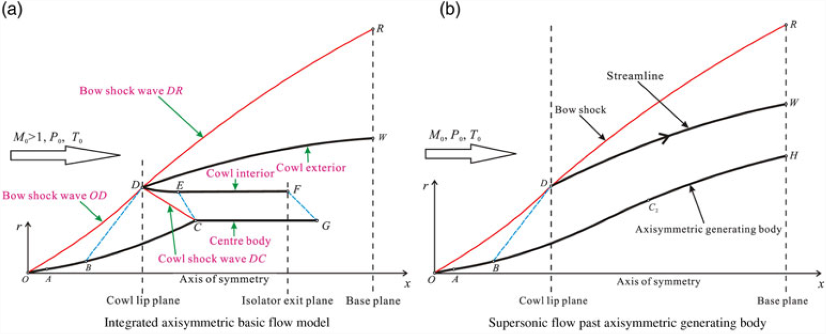
Inspired by the above-discussed works on waverider airframe/inlet integration, Ding et al.(Reference Ding, Liu, Shen and Huang4) were the first to propose a novel airframe/inlet integration derived from an axisymmetric generating body. In their work, a new basic flow model (shown in Fig. 1(a)) considering both internal and external flows was derived from an axisymmetric generating body by use of both the streamline tracing and the method of characteristics (MOC). Subsequently, the airframe/inlet integrated waverider vehicle was developed from the basic flow model by the streamline tracing method. The design concept of the basic flow model derived from an axisymmetric generating body is as follows. First, an axisymmetric generating body (OH) is taken as the initial condition, and a shock wave (OR) is generated around the axisymmetric generating body (OH) under supersonic inflow conditions, as shown in Fig. 1(b). Then, the streamline (DW) passing through the inlet lip (D) is used as the cowl exterior of the basic flow model, as shown in Fig. 1(a). The axisymmetric shock wave (OR) is divided by the cowl exterior into the forebody shock wave (OD) and the afterbody shock wave (DR). A reflected shock wave (DC) is produced at the lip when the forebody shock wave (OD) hits the inlet lip; then, the air is compressed into the inlet by the cowl interior (DEF). The afterbody shock wave (DR) is attached to the cowl lip, and the flow field between the afterbody shock wave (DR) and the cowl exterior (DW) is used to design the afterbody of the integrated vehicle. The major shortcoming of this model is that the design freedoms of the forebody shock wave (OD) and that of the afterbody shock wave (DR) are limited because the shock wave (OR) is generated from an axisymmetric generating body.
Schematic illustration of the airframe/inlet integrated axisymmetric basic flow model derived from the axisymmetric generating body(Reference Ding, Liu, Shen and Huang4).

With the aims of overcoming the above-described limitations of the basic flow model derived from an axisymmetric generating body and extending the design freedom of the airframe/inlet integrated waverider vehicle, the present study first develops an upgraded basic flow model derived from an axisymmetric shock wave and then upgrades the design method of the airframe/inlet integration on the basis of an axisymmetric shock wave. In this paper, first, the upgraded design principle and method for the airframe/inlet integrated waverider vehicle based on an axisymmetric shock wave are described in detail. Second, an upgraded basic flow model is derived from an axisymmetric shock wave; the design concept, method, and procedure for this upgraded basic flow model are described in detail. Third, a test case designed by the updated airframe/inlet integration design methodology is solved; numerical computation methods employed to validate the upgraded design method, and analyse the performances and viscous effect of the vehicle are presented. Moreover, it is worth noting that as the osculating cone concept has not been considered in the design of the proposed full-waverider vehicle, the shock wave profile of the bottom cross-section of the waverider forebody can only be limited to an arc curve, but can not be rationally designed according to the shape of the inlet lip. This limitation is not conducive to the airframe/inlet integration. We intend to apply the osculating cone concept to the future optimisation design of the full-waverider vehicle. The use of the osculating cone concept will greatly expand the design space and application range of the full-waverider vehicle.
2.0 DESIGN METHOD OF A FULL-WAVERIDER VEHICLE
2.1 Constitutive parts and basic flow model
The vehicle developed according to the proposed design concept is termed the ‘airframe/inlet integrated full-waverider vehicle’ in this study, or the ‘full-waverider vehicle’ for short.
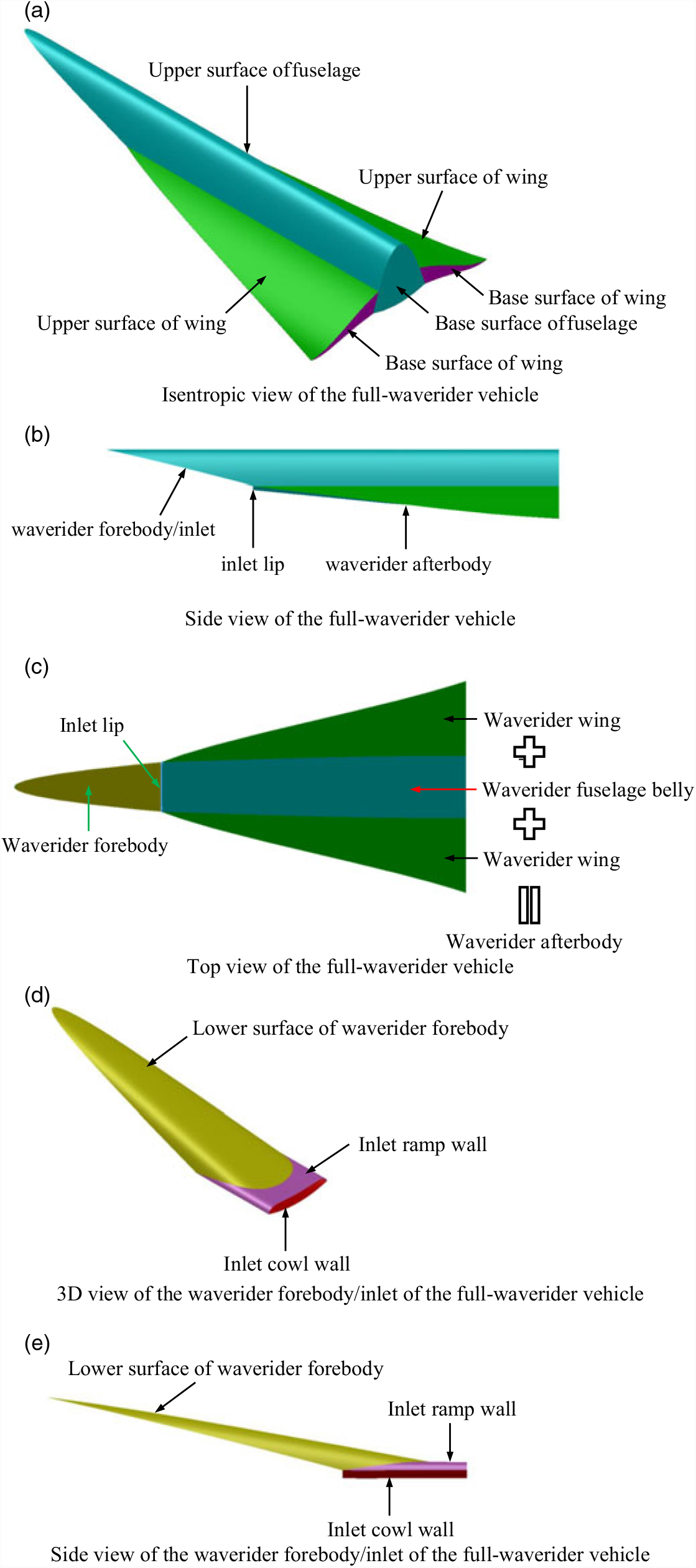
As shown in Figs. 2(a)–2(e), both the waverider forebody/inlet and the waverider after-body make up the full-waverider vehicle, and are connected at the inlet lip. The waverider afterbody is composed of a waverider fuselage belly and two waverider wings; in this study, the afterbody is defined as the part of the fuselage after the inlet lip and the two wings. In other words, the waverider surface of the full-waverider vehicle consists of the waverider forebody, waverider fuselage belly, and two waverider wings.
Constitutive parts of the full-waverider vehicle.

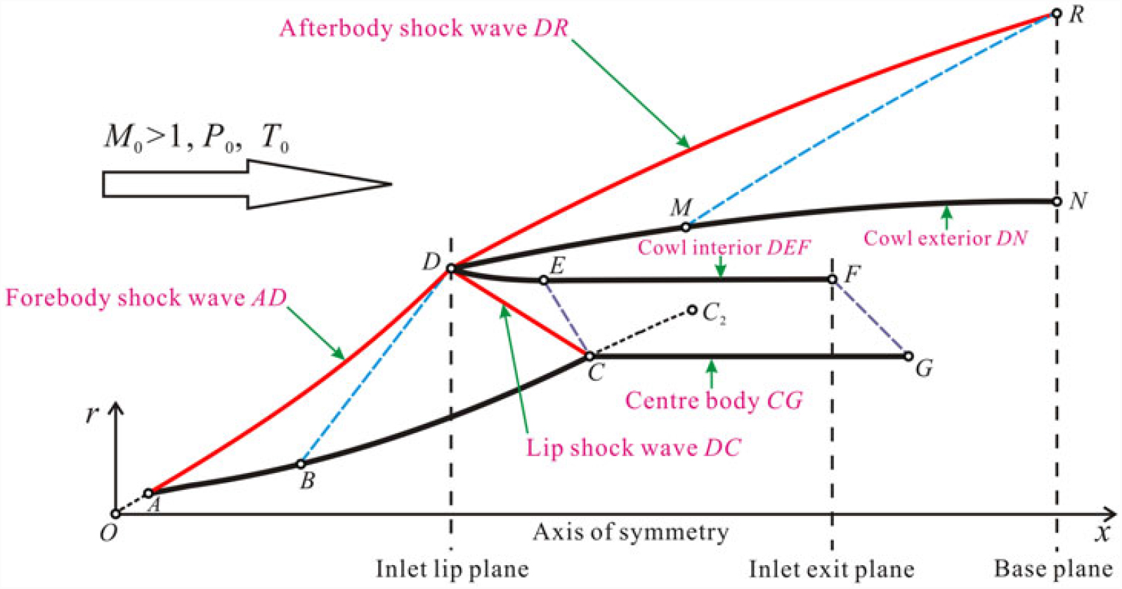
Both the waverider forebody/inlet and the waverider afterbody of the full-waverider vehicle are derived from the same basic flow model. Figure 3 illustrates the upgraded basic flow model derived from an axisymmetric shock wave; four walls and three curved shock waves constitute this model. In detail, the shock waves of this model consist of the forebody shock wave OD, afterbody shock wave DR, and lip shock wave DC. Further, the walls of this model consist of the forebody wall ABC, centre body CG, cowl interior DEF, and cowl exterior DMN. The basic flow field of this model is divided into two regions by the cowl interior DEF and the cowl exterior DMN, namely, region A-B-C-G-F-E-D and region D-M-N-R. The region A-B-C-G-F-E-D is used as the basic flow field to generate the inlet and forebody; it is termed the forebody/inlet basic flow region. The region D-M-N-R is used as the basic flow field to generate both the fuselage belly and two wings, which constitute the afterbody of the vehicle; this region is termed the afterbody basic flow region. Moreover, the lip shock wave is required to cancel at shoulder point C (located on the centre body) while reorienting the flow field to align it with the angle of the centre body.
Schematic illustration of the airframe/inlet integrated axisymmetric basic flow model derived from the axisymmetric shock wave.

This upgraded basic flow model derived from an axisymmetric shock wave shown in Fig. 3 differs from the model derived from an axisymmetric generating body shown in Fig. 1. In the model shown in Fig. 1, the shock wave OR is generated from the axisymmetric generating body, and then, this shock wave is divided into two segments, namely, the forebody shock wave OD and the afterbody shock wave DR. Therefore, the two shock waves maintain curvature continuity at the lip point D. However, this curvature continuity reduces the design freedom of these two shock waves. On the contrary, in the model shown in Fig. 3, the two shock waves OD and DR do not need to maintain curvature continuity at the lip point D. Therefore, the shape and position of these two shock waves can be independently designed according to design requirements; in other words, the shock wave intensity can be effectively controlled. This advantage extends the design freedom of the basic flow model, which, in turn, extends the design freedom of the full-waverider vehicle.
2.2 Design principle and method
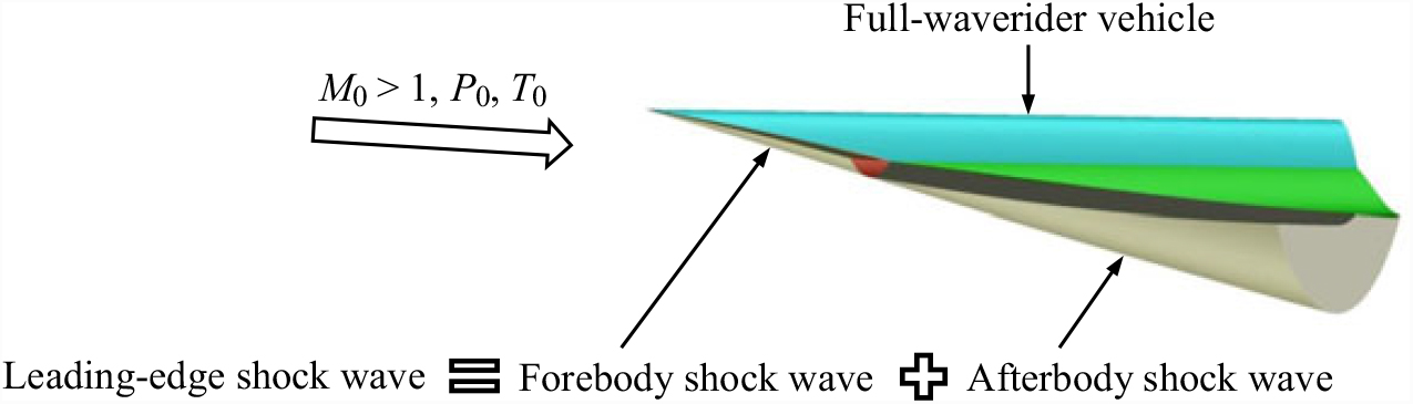
Figure 4 shows the 3D effect diagram of the full-waverider vehicle. It can be seen that the leading-edge shock wave is attached to the inlet lip and the leading edge of the vehicle. The leading-edge shock wave consists of the forebody shock wave and the afterbody shock wave. Under the designed flight conditions, the forebody of the full-waverider vehicle rides on the forebody shock wave (i.e. forebody waverider), and its two wings and fuselage belly ride on the afterbody shock wave (i.e. afterbody waverider); the forebody waverider and the after-body waverider together constitute the ‘full-waverider’. In other words, the entire vehicle can ride on the leading-edge shock wave, which causes the leading-edge shock wave to remain attached to the leading edge for the entire length of the full-waverider vehicle; this consequently prevents the higher-pressure air on the lower surfaces from spilling over the leading edge to the upper surface with lower-pressure air. This feature enables the vehicle design to take full advantage of the waverider’s high lift-to-drag ratio characteristics. At the same time, the inlet lip is also attached to the forebody shock wave; in other words, the forebody/inlet maintains the shock-on-lip condition under the design flight condition, thus enabling the inlet to efficiently capture the precompressed air flow.
Schematic representation of the full-waverider vehicle and corresponding attached leading-edge shock wave.

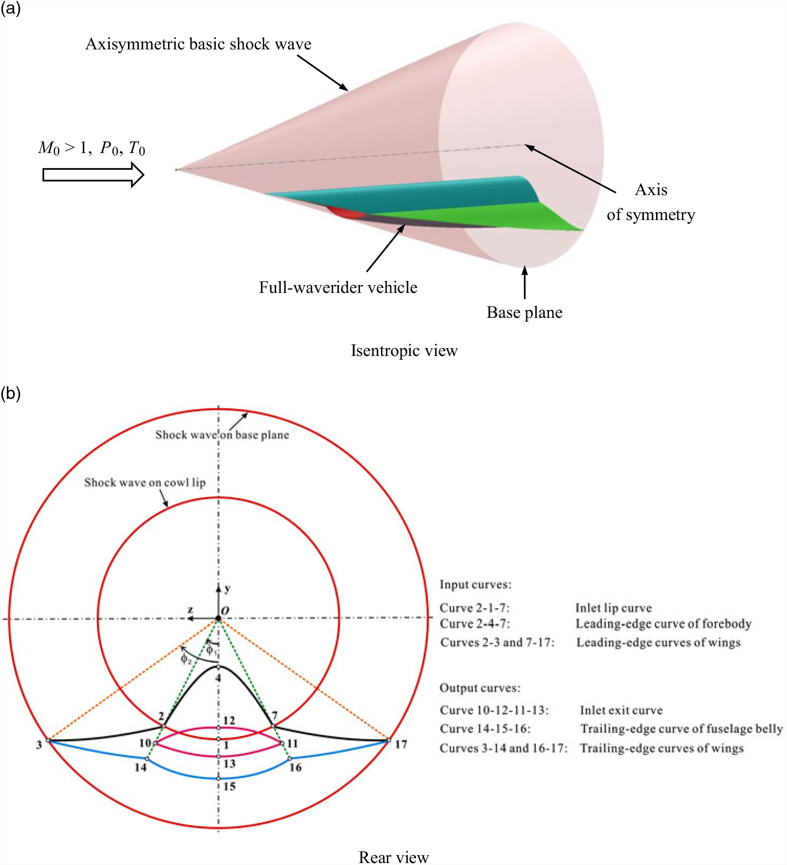
Figure 5 illustrate the basic design principle of the airframe/inlet integrated full-waverider methodology. As shown in Fig. 5(a), under supersonic inflow conditions, an axisymmetric basic shock wave is taken as the initial condition, and then, both the waverider forebody and the waverider afterbody of the full-waverider vehicle are generated in the 3D flow field after the axisymmetric basic shock wave. As mentioned earlier, the waverider afterbody is composed of the waverider fuselage belly and two waverider wings. As shown in Fig. 5(b), the forebody/inlet is generated by tracing the streamlines in the forebody/inlet basic flow region (i.e. region A-B-C-G-F-E-D as shown in Fig. 3), from the leading-edge curve of forebody (curve 2-4-7) and the inlet lip curve (curve 2-1-7) downstream, up to the inlet exit plane; this simultaneously yields the inlet exit curve (curve 10-12-11-13). Then, the waverider surfaces of the fuselage belly and two wings are generated by tracing the streamlines in the afterbody basic flow region (i.e. region D-M-N-R as shown in Fig. 3), from the inlet lip curve (curve 2-1-7) and the leading-edge curves of two wings (curves 3-2 and 7-17) downstream, up to the base plane; this also simultaneously yields the trailing-edge curve of the fuselage belly (curve 14-15-16) and the trailing-edge curves of two wings (curves 3-14 and 16-17).
Schematic representation of the full-waverider vehicle and corresponding axisymmetric basic shock wave.

For simplicity, as done previously for the design of an airframe/inlet integrated waverider(Reference Ding, Liu, Shen and Huang4), the blending upper surface of fuselage and two wings is considered to remain a free-stream surface. The advantage of the free-stream upper surface is that the free-stream flow field on the upper surface will not affect the ‘waverider characteristics’ of the lower surface of the waverider vehicle at zero angle-of-attack of the specified design condition. However, the disadvantage of the free-stream upper surface is that the volume efficiency of the waverider vehicle is not high, which is not conducive to improving the payload capacity of the waverider vehicle. In the future, a compression surface(Reference Takashima and Lewis44,Reference Takashima45) may be used as the upper surface to further improve the volume efficiency and payload capacity of the full-waverider vehicle. We intend to study this problem in more detail in a future optimization design of the full-waverider vehicle.
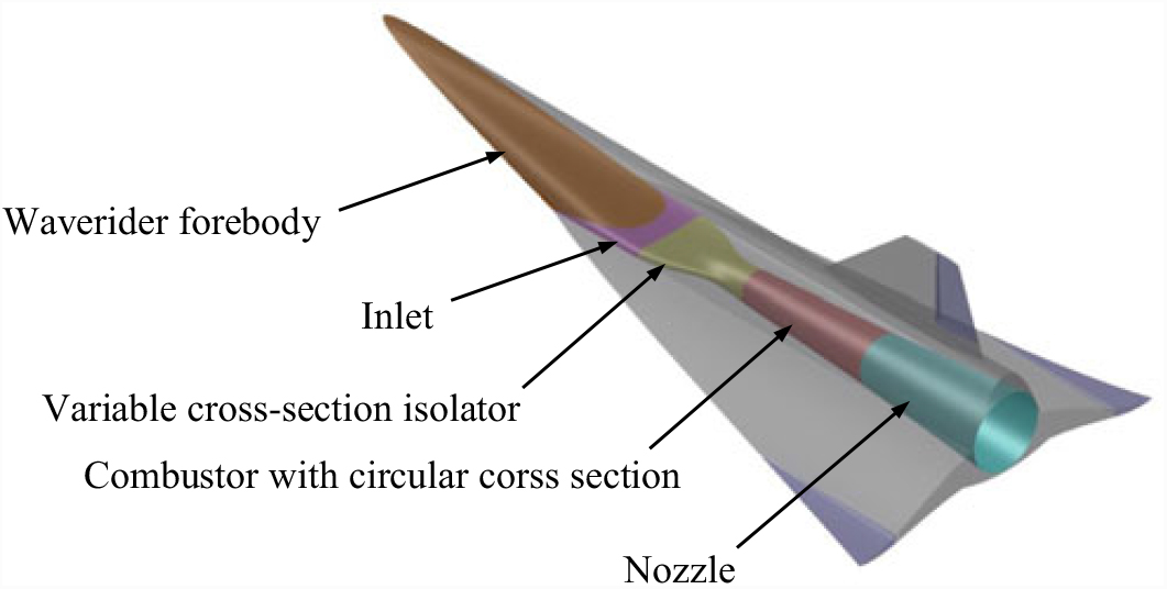
It is worth noting that for an airbreathing hypersonic vehicle, the matching design between the inlet and the combustor is a very important issue. In order to solve the matching problem between the inlet designed in this paper and combustor, a variable cross-section isolator may be used. The entrance shape of the variable corss-section isolator is the exit contour of the inlet, while the exit shape of the variable corss-section isolator is the entrance contour of the combustor. If the combustor is of a circular cross section, the preliminary conception of the whole internal flow passage is shown in Fig. 6. We intend to study this problem in more detail in a future optimisation design of the full-waverider vehicle.
Preliminary conception of whole internal flow passage of full-waverider vehicle.

2.3 Design procedure of the basic flow model
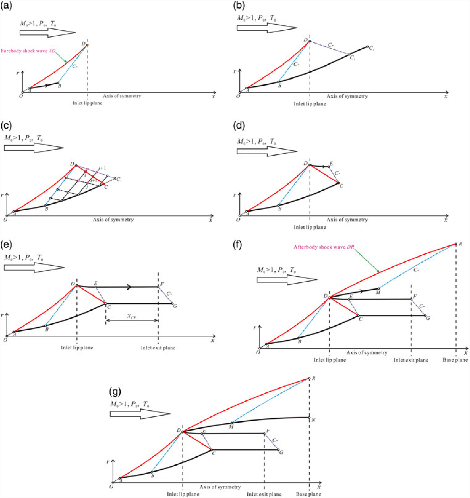
In order to overcome the limitations of the existing basic flow model derived from an axisymmetric generating body and extend the design freedom of the full-waverider vehicle, a upgraded basic flow model derived from an axisymmetric basic shock wave is utilised by use of both the MOC(Reference Zucrow and Hoffman46,Reference Kothari, Tarpley, Mclaughlin, Babu and Livingston47) and the streamline tracing method(Reference Billig and Kothari48). As shown in Fig. 7(a)-(g), the following procedure can generate this upgraded basic flow model:
Schematic illustration of the method and procedure used to design and solve the upgraded basic flow model.

(1) Figure 6(a) illustrates the method determining the flow parameters (M, P, T, θ) of the forebody-shock-wave-dependent region A-B-D and the position of wall AB. First, a curve AD is designed as the forebody shock wave. Then, given the position and shape of the forebody shock wave AD, and the design condition (M 0, P 0, T 0) at the zero angle-of-attack, the region A-B-D can be determined by the MOC and the streamline AB can be obtained using the streamline tracing method. The cross section that passes through point D is taken as the inlet lip plane, and DB is a left-running Mach line. Then, the streamline AB is used as the front segment of the forebody wall.
(2) Figure 6(b) illustrates the method used to determine the flow parameters (M, P, T, θ) of the isentropic compression region B-C 1-D. First, a curve BC 2 is designed as the isentropic compression wall. Then, given the position of the wall BC 2 and the flow parameters (M, P, T, θ) of the left-running Mach line DB (solved in step (1) of this procedure), the region B-C 1-D can be determined by the MOC, and DC 1is a right-running Mach line. The region B-C 1-D can be used to determine the positions of the lip shock wave DC and the flow parameters just downstream of it.
(3) Figure 6(c) illustrates the method determining the positions of the lip shock wave DC and the flow parameters (M, P, T, θ) just downstream of it. In the region B-C 1-D, the right-running and left-running Mach lines are represented by the dashed and thin lines, respectively. The intersection points of these lines and the shock wave points in the lip shock wave DC are represented by the hollow and solid nodes, respectively. The positions and flow parameters at these hollow nodes can be solved by the MOC. Given the flow angle distribution just downstream of the lip shock wave DC [expressed by Eq. (1)], the nodal positions of the lip shock wave DC and the flow parameters just downstream of it can be solved by the predictor-corrector method. For a detailed description of the method and procedure, please refer to our previous work(Reference Ding, Liu, Shen and Huang4).
(1) $$\theta _{DC,2} = \theta _{DC,2} \left( x \right),\;x \in \left[ {x_D ,x_C } \right]$$
Here, θ DC,2 is the distribution of the flow angle θ as a function of x just downstream of the lip shock wave DC.
(4) Figure 6(d) illustrates the method for determining the positions of the wall DE. When the positions of the lip shock wave DC and flow parameters just downstream of it are solved (as described in step (3) of this procedure), the region D-C-E can be determined by the MOC and the streamline DE can be obtained using the streamline tracing method. Additionally, CE is the right-running Mach line. Then, the streamline DE is used as the front segment of the inner wall of the cowl.
(5) Figure 6(e) illustrates the method determining the positions of the wall EF. Given the distributions of the Mach number and the angle of the slope along the wall CG expressed by Eqs. (2) and (3), respectively, and the distance along the x-direction between points C and F (x CF), the region E-F-G-C can be determined by the MOC and the streamline EF can be solved using the streamline tracing method. A right-running Mach line (GF, originating from point G) intersects the streamline EF at point F. Moreover, in order to ensure that the lip shock wave DC cancels at point C, the flow angle just downstream of the lip shock wave DC at point C is required to be equal to the angle of the slope of the curve CG estimated at point C. The streamline EF is used as the back segment of the inner wall of the cowl. The streamlines DE and EF together constitute the inner wall of the cowl, which is termed the cowl interior DEF in Fig. 3.
(2)$$M_{CG} = M_{CG} \left( x \right),\;x \in \left[ {x_C ,x_G } \right]$$
(3)$$\delta _{CG} = \delta _{CG} \left( x \right),\;x \in \left[ {x_C ,x_G } \right]$$
Here, M CG and δ CG are, respectively, the distributions of the Mach number and the angle of the slope along the wall CG, and these two parameters are all functions of x.
(6) Figure 6(f) illustrates the method used to determine the position of the wall DM and the flow parameters (M, P, T, θ) of the afterbody-shock-wave-dependent region D-M-R. First, a curve DR is designed as the afterbody shock wave. Then, given the position and shape of the afterbody shock wave DR and the design condition (M 0, P 0, T 0), the region D-M-R can be determined by the MOC and the streamline tracing method. DM can be obtained by the streamline tracing method. The cross section passing through point R is utilised as the base plane of the basic flow model, and RM is a left-running Mach line. Then, the streamline DM is used as the front segment of the outer wall of the cowl.
(7) Figure 6(g) illustrates the method used to determine the flow parameters (M, P, T, θ) of the isentropic compression or expansion region M-N-R. First, a curve MN is designed as the isentropic compression or expansion wall, and point N is set at the base plane. Then, given the position of the wall MN and the flow parameters (M, P, T, θ) of the left-running Mach line MR (solved in step (6) of this procedure), the region M-N-R can be determined by the MOC. The streamline MN is used as the back segment of the outer wall of the cowl. Both DM and MN together constitute the outer wall of the cowl, which is named cowl exterior DMN in Fig. 3.


As a result of this design procedure, the upgraded basic flow model is obtained, and the corresponding basic flow field used for the design of the full-waverider vehicle is generated.
3.0 PHYSICAL MODEL AND NUMERICAL METHOD
3.1 Physical model
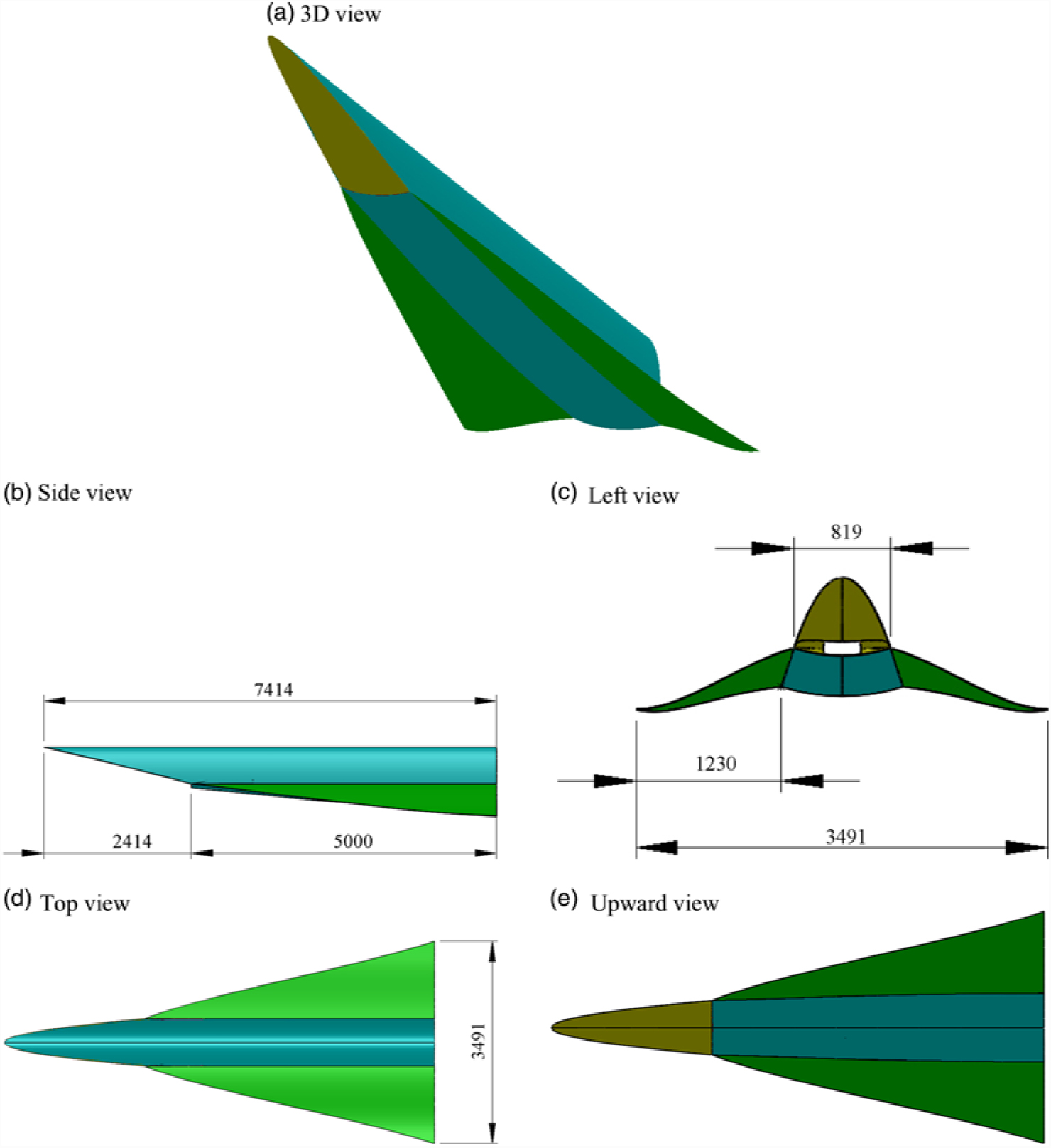
This section describes the method used to solve the practical case wherein the upgraded fullwaverider theory is employed and generation of the corresponding geometric model of the full-waverider vehicle in which the combustion chamber, nozzle, and control surfaces are not considered as done in our past work(Reference Ding, Liu, Shen and Huang4). Figure 7 shows the geometric model and size for the considered case. It can be seen from Fig. 8 that the length and width of the geometric model are about 7.4 m and 3.5 m, respectively, and the length of the forebody is about 2.4 m.
Geometric model for test case of full-waverider vehcle.

In this case, the inlet design parameters at the inlet exit plane of the basic flow model are an average Mach number and average pressure rise ratio at the inlet exit of about 3.8 and 10.0, respectively. A three polynomial curve is used as the forebody shock wave AD, a straight curve is used as the afterbody shock wave DR, and the design values of the shock wave angle at points A, D, and R are shown in Table 1. β A and β D is the shock wave angles of the forebody shock wave AD at point A and D, respectively, and β DR is the shock wave angle of the afterbody shock wave DR. The flow angles just downstream of the shock wave corresponding to β A, β D, and β DR are 6°, 8°, and 5°, respectively. The equation of the forebody shock wave AD is shown in Eq. (4). When the coordinate values (x, r) at points A, D, and R are given in Eq. (5)–(7), the forebody shock wave AD and the afterbody shock wave DR can be determined.
Design values of the shock wave angle used for the axisymmetric basic flow model of the full-waverider

 $$r = a_{AD} x^3 + b_{AD} x^2 + c_{AD} x + d_{AD} ,x \in [x_A ,x_D ]$$
 $$\left\{ {\matrix{{r_A = 0.1r_D } \hfill \cr {x_A = {{r_A } \over {\tan \left( {\beta _A } \right)}}} \hfill \cr } } \right.$$
 $$\left\{ {\matrix{{x_D = 5.0m} \hfill \cr {r_D = x_D \tan \left( {{{\beta _A + \beta _D } \over 2}} \right)} \hfill \cr } } \right.$$
 $$\left\{ {\matrix{{x_R = 10.0m} \hfill \cr {r_R = r_D + \left( {x_R - x_D } \right)\tan \left( {\beta _{DR} } \right)} \hfill \cr
} } \right.$$
A straight curve is used as the wall BC 2, and the coordinate values (x, r) at point C 2 are given in Eq. (8).
 $$\left\{ {\matrix{{x_{C_2 } = 7.0m} \hfill \cr {r_{C_2 } = r_B + \left( {x_{C_2 } - x_B } \right)\tan \left( {\delta _B } \right)} \hfill \cr
} } \right.$$
where δ B is the angle of slope at the wall point B, which can be determined by the forebody shock wave AD.
A three polynomial curve is used as the wall MN, and its equation is shown in Eq. (9). When the first derivative of the wall MN at point M remains continuous, and the angle of slope d and the r coordinate at point N are given in Eq. (10), the wall MN can be determined.
 $$r = a_{MN} x^3 + b_{MN} x^2 + c_{MN} x + d_{MN} ,x \in \left[ {x_M ,x_N } \right]$$
 $$\left\{ {\matrix{{{\rm{r}}_N = r_M + 0.5\left( {x_N - x_M } \right)\tan \left( {\delta _M } \right)} \hfill \cr {\delta _N = 0^ \circ } \hfill \cr } } \right.$$
Table 2 lists the specific parameters for the basic flow model. As shown in Table 2, θ DC,2 is the distribution of the flow angles θ just downstream of the lip shock wave DC; M CG and δ CG are the distributions of the Mach number and the angle of the slope along the wall CG, respectively, and the condition M CG (x) = M C means that the Mach numbers along the wall CG are equal to the Mach number at the point C; x CF is the distance from the inlet exit plane to point C along the x axis direction, and the length 1.3 m chosen in this case is about 8 times of the inlet height at the inlet exit plane. The static pressure P 0 and the static temperature T 0 in Table 2 correspond to the atmosphere parameters of 25 km.
Specific parameters used for the axisymmetric basic flow model of the full-waverider

As shown in Fig. 5(b), the input curves used for the design of the full-waverider vehicle include the inlet lip curve (curve 2-1-7), the leading-edge curve of forebody (curve 2-4-7) and the leading-edge curve of two wings (curve 2-3, 7-17). In this case, the leading-edge curves of the forebody and two wings are expressed by the projection curves of the leading-edge curves on the base plane, and both the leading-edge curves and the corresponding projection curves are marked with the same notations for convenience. The output curves obtained by tracing the streamlines in the basic flow model include the inlet exit curve (curve 10-12-11-13), the trailing-edge curve of fuselage belly (curve 14-15-16) and the trailing-edge curves of two wings (curve 3-14, 16-17).
A quadratic curve is selected as the projection curve of the leading-edge curve of forebody (curve 2-4-7), and it is expressed by Eq. (11). When the coordinate values (z, y) at point 4 and point 2 are given in Eq. (12), the curve 2-4-7 can be determined.
 $$y = a_{4 - 2} + b_{4 - 2} z^2 ,\;\;z \in \left[ {0,z_2 } \right]$$
 $$\left\{ {\matrix{{z_4 = 0.0,\;y_4 = - 0.5r_D } \hfill \cr {z_2 = r_D \sin \phi _1 ,\;y_2 = - r_D \cos \phi _1 } \hfill \cr {\phi _1 = 18^ \circ } \hfill \cr } } \right.$$
where r D represents the shock wave radius of the basic flow model at the inlet lip plane, and its value is shown in Eq. (6).
A quartic curve is selected as the projection curve of the leading-edge curve of the wings (curve 2-3, 7-17), and its equation is shown in Eq. (13). When the angle of the slope at the point 3 is zero degrees, and the coordinate values (z, y) at point 2 and point 3 are given in Eq. (14), the curve 2-3 and 7-17 can be determined.
 $$y = a_{2 - 3} + b_{2 - 3} z^2 + c_{2 - 3} z^4 ,z \in \left[ {z_2 ,z_3 } \right]$$
 $$\left\{ {\matrix{{z_2 = r_D \sin \phi _1 ,\;y_2 = - r_D \cos \phi _1 } \hfill \cr {z_3 = r_R \sin \phi _2 ,\;y_3 = - r_R \cos \phi _2 } \hfill \cr {\phi _1 = 18^ \circ } \hfill \cr {\phi _2 = 44.427^ \circ } \hfill \cr {\left( {{{dy} \over {dz}}} \right)_{z = z_3 } = 0} \hfill \cr } } \right.$$
where r R represents the shock wave radius of the basic flow model at the base plane, and its value is shown in Eq. (7).
3.2 Numerical methods
As done previously for the numerical simulation of a waverider(Reference Ding, Liu, Shen and Huang4,Reference Ding, Shen, Liu and Huang9,Reference Ding, Shen, Liu and Huang11) , in this study, the two-equation shear-stress transport (SST) k-ω turbulence model and the 3D coupled implicit Reynolds-averaged Navier–Stokes (RANS) equations are employed to numerically simulate the viscous aerodynamic performance and flow fields of the basic flow model and the fullwaverider vehicle by use of ANSYS Fluent(49). The second-order spatially accurate upwind scheme applying the AUSM to flux vector is used, and the Green–Gauss cell-based gradient method is utilised to compute the gradients. A Min-mod (Minimum Modulus) limiter derived from the work of Barth and Jespersen(Reference Barth and Jespersen50) is implemented as the gradient limiter to control the discontinuous pressure jumps at the shock front. This limiter is of a non-differentiable type and uses the Min-mod function to limit and clip the reconstructed solution overshoots and undershoots on the cell faces(49). The CFL number is set at 0.5. The enhanced wall treatment(49) is applied to the flow in the near-wall region in the selected model, and the no-slip velocity boundary condition is imposed along the walls of the model(Reference Huang, Wang, Pourkashanian, Ma, Ingham, Luo, Lei and Liu51). The thermal boundary condition at the walls is considered to be adiabatic in this study(Reference Huang and Wang52). The air is assumed to be a thermally and calorically perfect gas(Reference Huang, Liu, Li, Xia, Liu and Wang53), and its viscosity is modelled according to the Sutherland law(Reference Mansour and Khorsandi54), which is expressed by Equation (15)(Reference Chen, Hou, Liu and Gao55). The thermal conductivity of the gas is determined by the Prandtl number, and it is expressed by Eq. (16)(Reference Liu, Hou, Chen and Zhang56). The specific heat ratio γ is also assumed to be a constant value of 1.4 in this study(Reference Roy and Blottner57).
 $$\mu = 1.458 \times 10^{ - 6} {{T^{1.5} } \over {T + 110.4}}$$
 $$k = {{\mu C_p } \over {\Pr }}$$
where μ is the dynamic viscosity coefficient; T is the static temperature of the air, expressed in Kelvin; k is the thermal conductivity of the gas; C p is the specific heat at constant pressure; and Pr is the Prandtl number.
The iterative process and its solutions can be considered to converge if the residuals attain minimum values, that is values less than four orders of magnitude of their original value, and when the difference between the computed inflow and outflow mass fluxes falls below 0.1%.
Euler equations are employed to numerically simulate the inviscid flow fields in the same problem formulation by use of ANSYS Fluent(49). The Euler equations are solved using the density-based (coupled) implicit solver. The second-order spatially accurate upwind scheme applying the AUSM to the flux vector is used, and the least-squares cell-based method is utilised to compute the gradients. The CFL number is set at 0.5. As indicated previously, the air is assumed to be a thermally and calorically perfect gas. Convergence is assumed to be achieved under the same conditions as those described above.
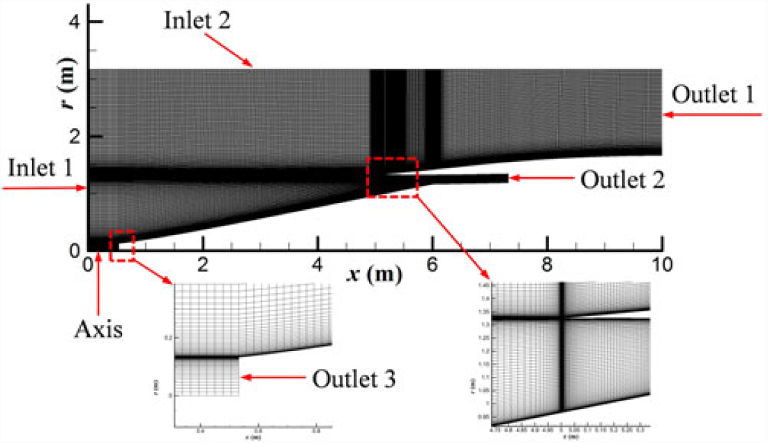
The structured grid and the inflow and outflow boundary conditions employed in the computational test of the basic flow model are shown in Fig. 9. In this figure, the pressure far-field is assigned as the boundary condition of inlet 1 and inlet 2, and the pressure outlet is assigned as the boundary condition of outlet 1, outlet 2, and outlet 3. Because of the axial symmetry of the geometric configuration, only a 2D flow field is required to be solved, and the number of structured grid cells is 122,894.
Schematic diagram of the structured grid and boundary conditions employed in the computational test of the airframe/inlet integrated axisymmetric basic flow model.

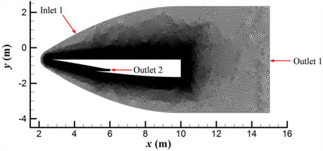
The unstructured grid and the inflow and outflow boundary conditions employed in the computational test of the full-waverider vehicle are shown in Fig. 10. Similarly to Fig. 9, in Fig. 10, the pressure far-field is assigned as the boundary condition of inlet 1 and the pressure outlet is assigned as the boundary condition of outlet 1 and outlet 2. Because of the symmetry of the geometric configuration, only half of the flow field is required to be solved, and the number of unstructured grid cells is 5,017,999.
Schematic diagram of the unstructured grid and boundary conditions employed in the computational test of the full-waverider vehicle (plane of symmetry).

As in our previous work(Reference Ding, Liu, Shen and Huang4), the specified design condition of the vehicle in this study is as follows: a cruising height of 25km, a flight Mach number of 6.0, and zero angle-of-attack.
3.3 Code validation
As done previously for the numerical simulation of a waverider(Reference Ding, Liu, Shen and Huang4,Reference Ding, Shen, Liu and Huang9,Reference Ding, Shen, Liu and Huang11) , two cases—case 1 and case 2—are considered to complete the code validation in order to investigate the accuracy of the numerical methods employed in this study.
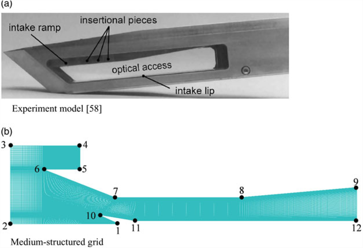
In case 1, a hypersonic inlet(Reference Reinartz, Herrmann and Ballmann58) used in our previous work on internal flows(Reference Ding, Shen, Huang and Liu59) is employed to discuss the present code program; its experimental model is shown in Fig. 11(a). The overall inlet geometry is based on similar inlet models tested within the framework of previous German studies(Reference Schmitz and Bissinger60). In the original model geometry proposed by such studies(Reference Schmitz and Bissinger60), two ramps deflect the flow before it enters the inlet. However, because of the restrictions of the wind tunnel used in Ref. Reference Reinartz, Herrmann and Ballmann58, the experimental setup requires the first outer compression ramp of the inlet geometry to be omitted in order to meet the specified test conditions for the inlet study. For the second ramp of the inlet, the same design condition as that proposed in Ref. Reference Schmitz and Bissinger60 is used (as the free-stream flow condition, also listed in Table 3) to permit testing of the relevant section in Ref. Reference Reinartz, Herrmann and Ballmann58.
Hypersonic inlet model for wind tunnel experiment and medium-structured grid used for numerical simulation.

Test conditions of hypersonic inlet model

In order to describe the locations of the specified boundary conditions employed in the hypersonic inlet model, the boundary points of the computational domain are numbered, as shown in Fig. 11(b); the specified boundary conditions are listed in Table 4. Three structured grid scales are introduced to analyse the grid independency in the numerical process: a coarse grid (497 × 66), a medium grid (994 × 130), and a refined grid (1,988 × 260). To ensure accuracy of the solution of turbulent flow, a y + value of less than 1 is used for the main portion of the wall flow region. Details relevant to the medium grid are also shown in Fig. 11(b).
Boundary conditions of computational domain for hypersonic inlet model

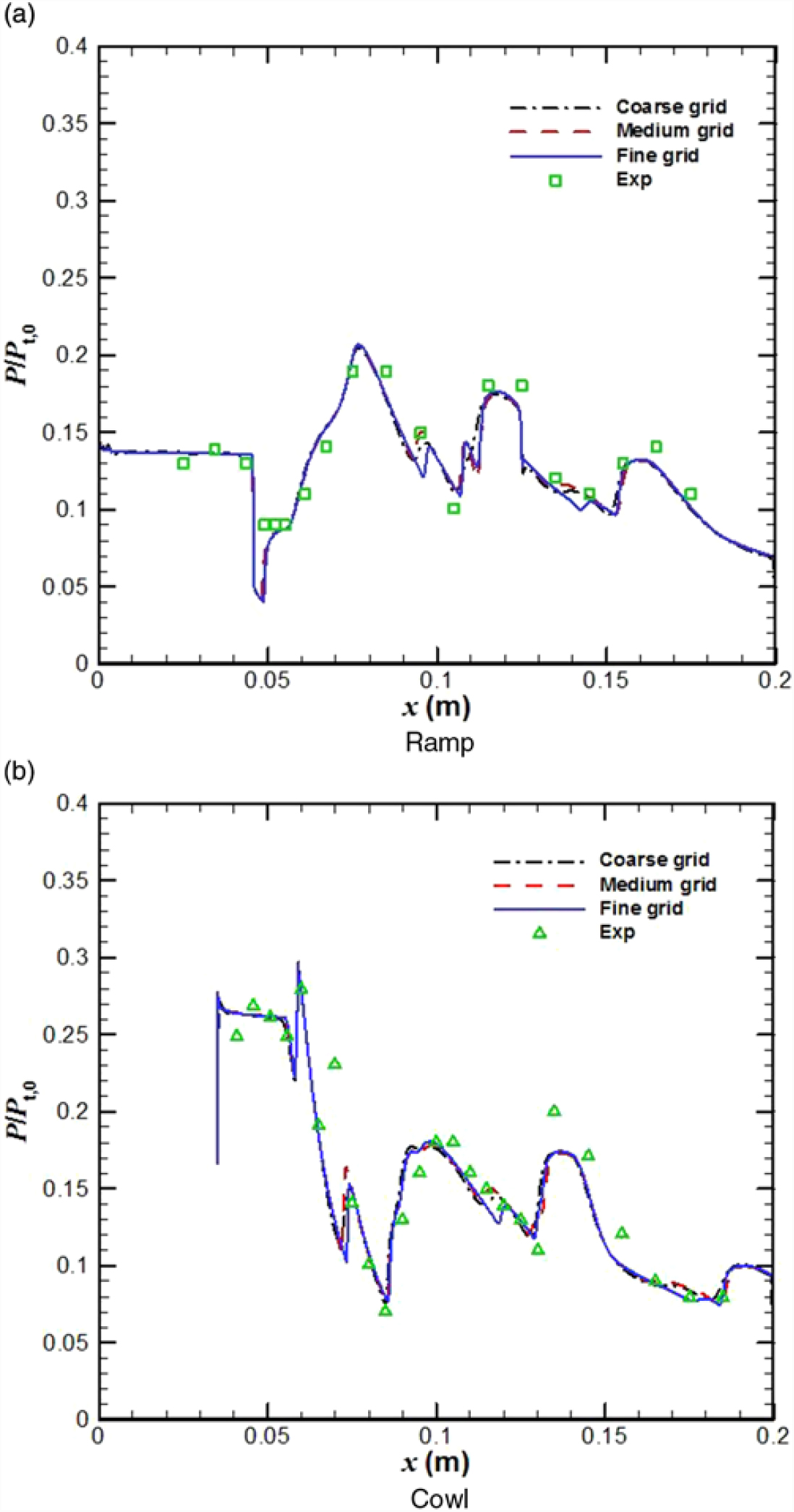
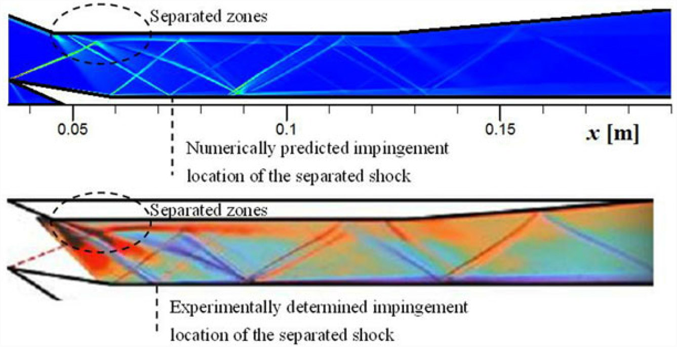
Fig. 12 shows a comparison of the pressure distributions along the cowl and on the ramp surfaces for the three grid scales, obtained using the SST k-ω turbulent model employed in the hypersonic inlet case. The numerical results obtained for the three grid scales are in good agreement with the experimental data, which confirms the grid independency in this hypersonic inlet case. Fig. 13 shows a comparison of the experimental schlieren image and the corresponding density gradient fields computed using the SST k-ω turbulence model, which also reveals good overall agreement between the numerical results and the experimental data. The shock wave pattern, separation, and approximate boundary-layer thickness in the schlieren image are all present in the predicted results. The computed separation zone appears smaller than that obtained experimentally, which makes the separation shock weaker and causes it to impinge downstream of the measurement location on the cowl surface. The reason for this discrepancy is probably the shortcoming in the existing two-equation turbulence model with regard to its tendency to under-predict the flow separation(Reference Huang and Coakley61). Overall, the computational results for the hypersonic inlet agree well with the physical aerodynamic concepts, and this not only reveals the intersection between the oblique shock waves and the expansion waves but also reflects the primary internal flow characteristics of a typical hypersonic inlet.
Comparison of wall pressure profiles at different grid scales employed in hypersonic inlet case.

Comparison of experimentally obtained schlieren image (bottom) and corresponding density gradient fields (top) obtained via computation using SST k-ω turbulence model.

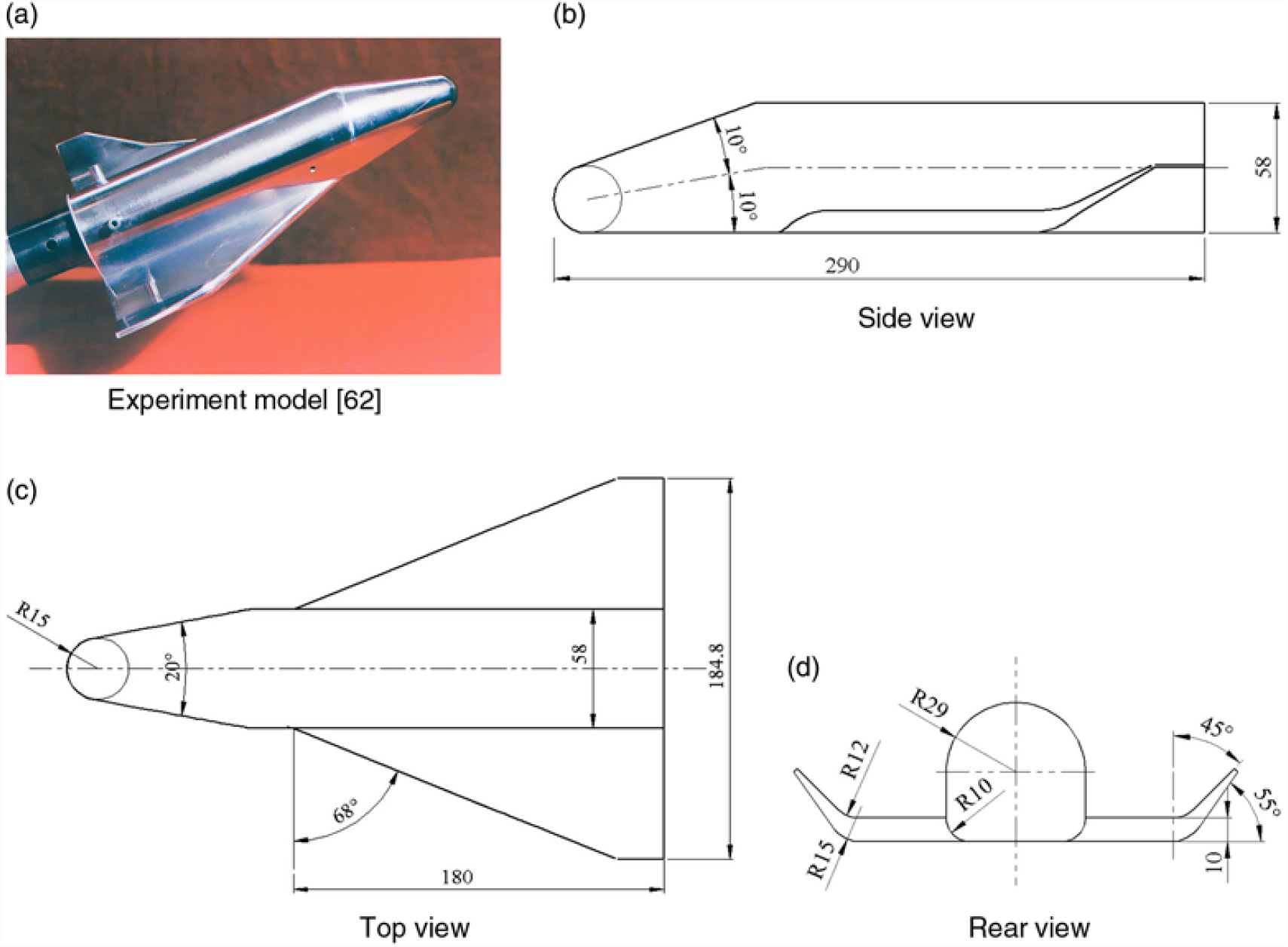
In case 2, the experiment model of the space shuttle(Reference Li62) [shown in Fig. 14(a)] in a wind tunnel is applied to validate the numerical simulations. The experimental model consists of three separate components: nose, fuselage, and two wings. Its body length is 290mm, maximum horizontal size is 184.8 mm, and maximum height is 58.0 mm. The detailed dimensions of the experimental model are provided in Figs. 14(b)–14(d).
Experimental model and three views of space shuttle used for wind tunnel experiments(Reference Li62) (unit: mm).

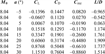
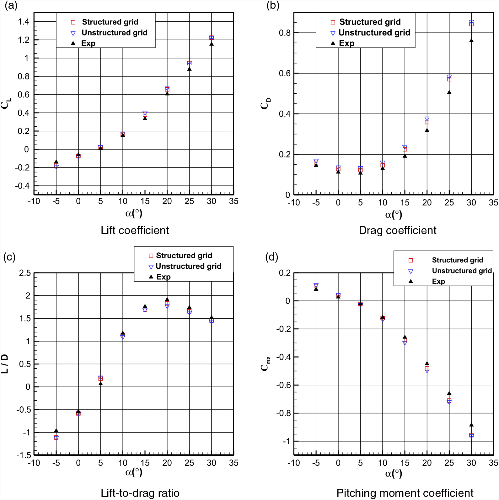
The boundary conditions for the free stream are set as follows in accordance with the experimental setup in Ref. Reference Li62: a Mach number of 8.04, a Reynolds number per unit length of 1.13 × 10⁷/m, a total pressure of 7.8MPa, and a total temperature of 892K. The detailed aerodynamic performance data of the space shuttle measured during the wind tunnel experiment(Reference Li62) are listed in Table 5. In this case, the reference length and area are 29.0 cm and 100.0 cm2, respectively. The reference point for the pitching moment coefficient given in Table 5 is the vertex of the space shuttle. In this study, a structured grid (3,753,594 cells), shown in Fig. 15(a), and an unstructured grid (4,938,688 cells), shown in Fig. 15(b), are introduced to analyse the grid independency. In the numerical process, the aerodynamic performances of the space shuttle for different angles of attack, ranging from –5° to 30° in increments of 5°, are obtained. The computational results obtained using the SST k-ω turbulence model for the two grids are compared with the experimental data, as shown in Fig. 16.
Aerodynamic performance data of space shuttle measured during wind tunnel experiment(Reference Li62)

Structured and unstructured grids used for numerical simulations of experimental space shuttle model.

Comparison of aerodynamic performances of space shuttle as calculated via numerical computation and measured during wind tunnel experiment.

It is clear that the lift coefficient, lift-to-drag ratio, and pitching moment coefficient obtained from the computations by using the structured grid and unstructured grid are in good agreement with the experimental data for the space shuttle under hypersonic flow conditions [see also Figs. 16(a), 16(c), and 16(d)]. When the angle-of-attack is no more than 15°, the drag coefficients obtained from the computations by using both the structured grid and the unstructured grid closely match the experimental data. When the angle-of-attack is larger than 15°, the numerical drag coefficients are slightly over-predicted, as shown in Fig. 16(b).
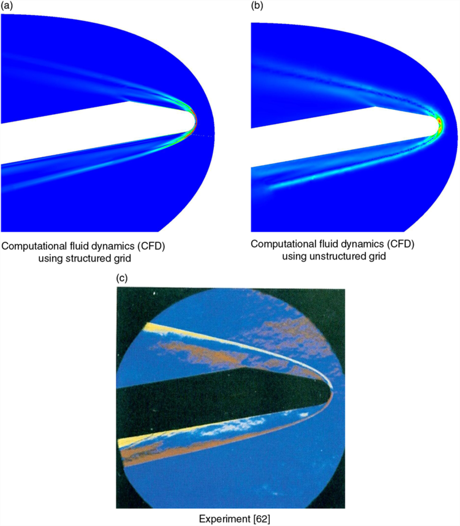
Fig. 17 shows a comparison of the experimental schlieren image and the corresponding density gradient fields computed using the SST k-ω turbulence model for the two grids employed in the space shuttle case, when the angle-of-attack is 10°. It is obvious that the numerical results obtained using the structured grid and unstructured grid are in good agreement with the experimental data. The positions of the shock wave are almost the same.
Comparison of experimental schlieren images and corresponding density gradient fields obtained via computation using SST k-ω turbulence model employed in space shuttle.

From the earlier discussion, it can be concluded that the numerical methods adopted in this study can simulate the hypersonic inlet and hypersonic vehicle within acceptable error margins and that the numerical results presented in Section 4 are plausible.
4.0 RESULTS AND DISCUSSION
4.1 Validation of upgraded basic flow model
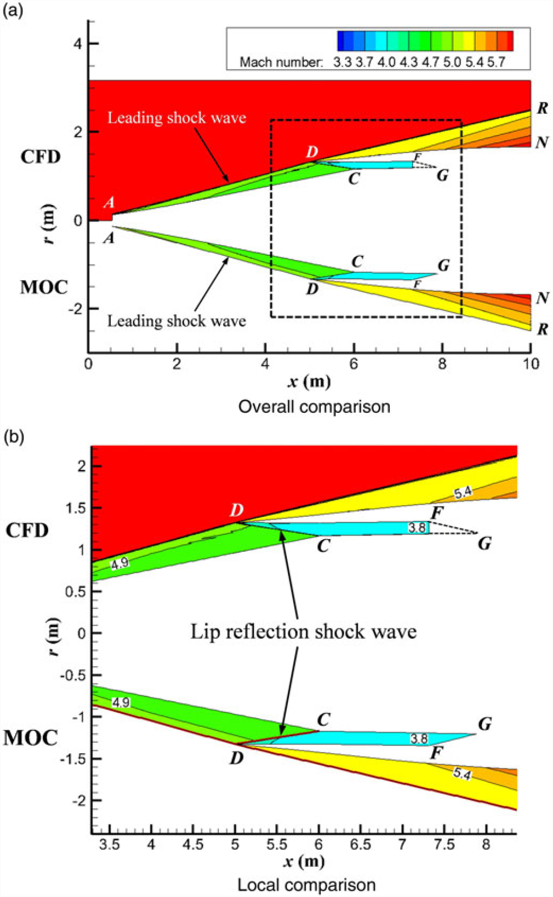
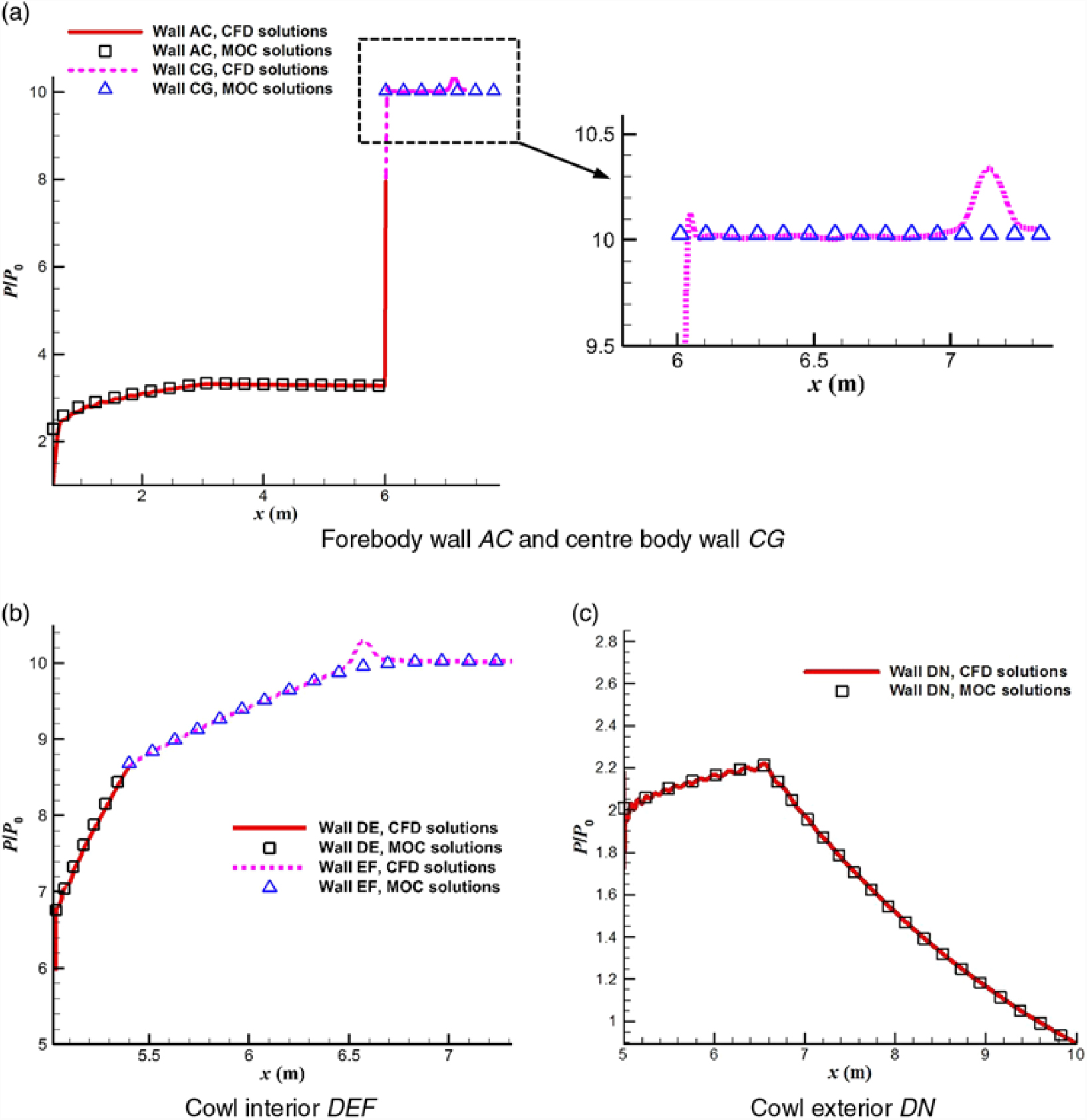
Figure 18 shows a comparison of the numerical Mach number flow field of the basic flow model for the upgraded basic flow model solved by the MOC and by the Euler solver, and Fig. 19 shows a comparison of the wall pressure distributions along the x-axis as solved by the MOC and by the Euler solver.
Comparison of numerical Mach number flow field of the basic flow model solved by the MOC and by the Euler solver.

Comparison of non-dimensional wall pressure distributions of the basic flow model solved by the MOC and by the Euler solver.

From Fig. 18, it is clear that the numerical flow fields solved by the MOC and by the Euler solver are approximately the same. No obvious reflected shock wave forms in the shoulder region of the isolator, that is cancellation of the lip shock wave DC at shoulder point C is achieved to meet the design requirements. From Fig. 19, it is obvious that there is no significant difference between the non-dimensional pressure distributions of the walls AC, DE, and DN solved by the MOC and by Euler solver. However, for the walls CG and EF, the pressure distributions solved by the Euler solver fluctuate near the values solved by the MOC. The possible reason for this difference is the defect of the Euler-solver-based method in mesh accuracy and shock wave resolution; specifically, the Euler-solver-based method creates a shock wave that smears over several grids, as a result of which a weak reflected shock wave may form in the shoulder region of the isolator in the numerical results obtained by the Euler-solver-based method, whereas an infinitely thin shock wave can be obtained by the MOC.
The above numerical analysis validates the design method of the upgraded basic flow model derived from an axisymmetric shock wave.
4.2 Validation of upgraded full-waverider vehicle design
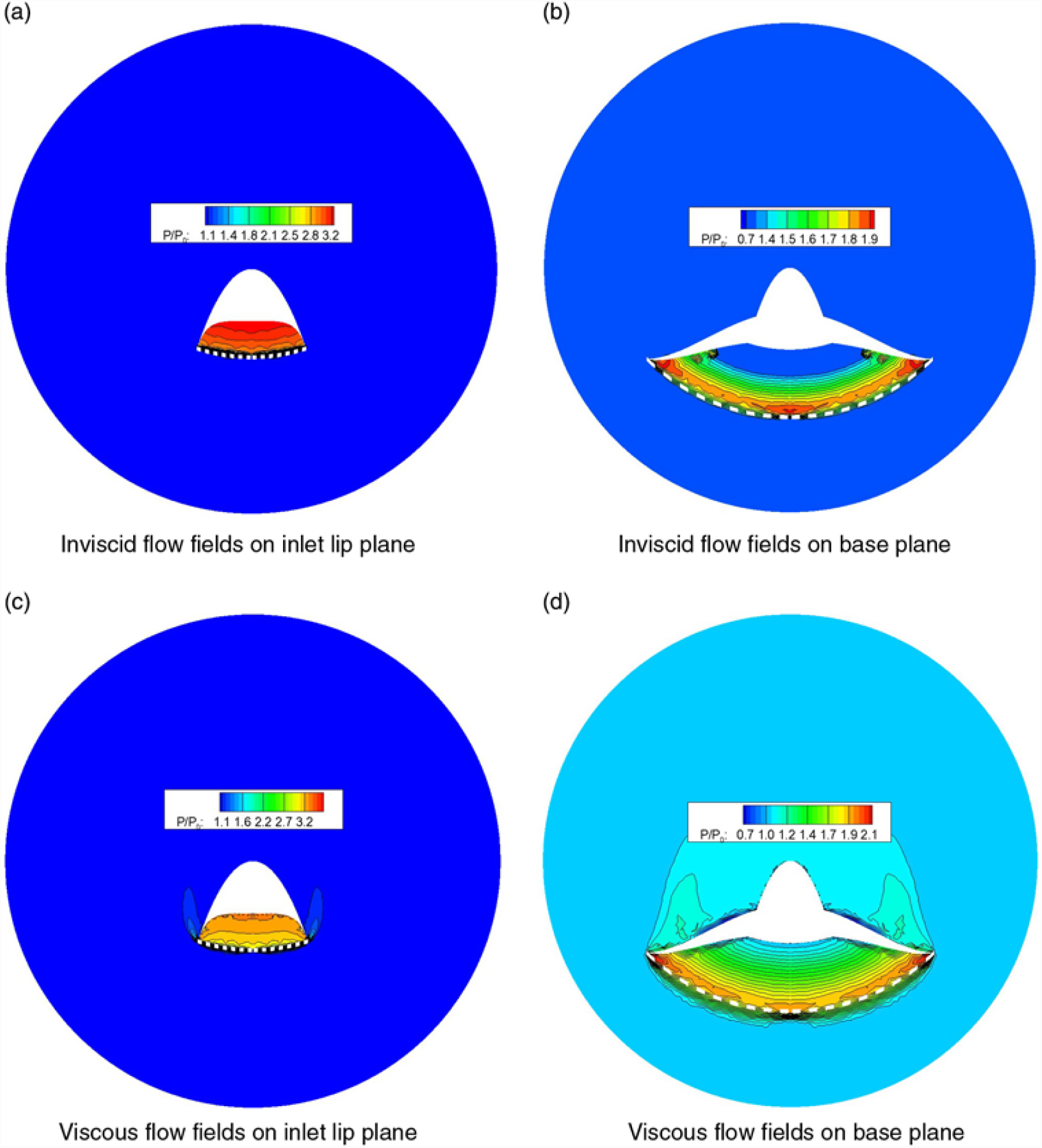
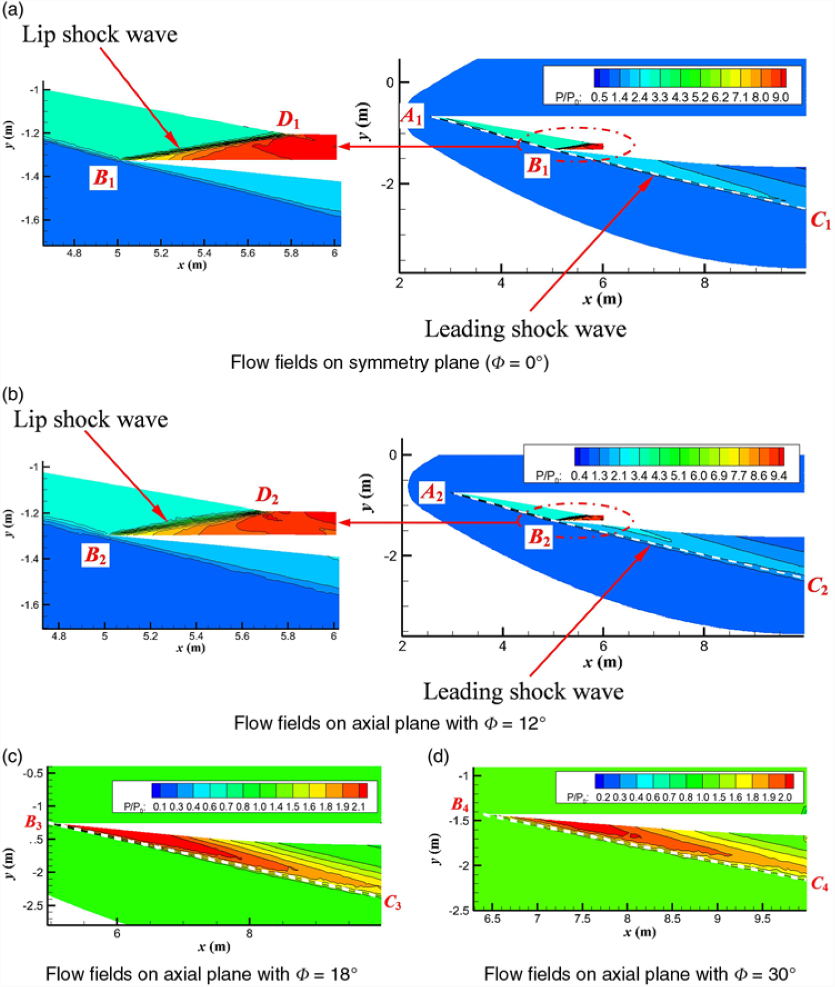
Figures 20(a), 20(b) and 21 show the inviscid flow fields on the inlet lip and base planes, and those on the axial planes of the full-waverider vehicle under the design condition, respectively. A comparison of the theoretical design and predicted shock wave locations is also shown in Figs. 20(a), 20(b) and 21, and the theoretical design shock wave locations are represented by the dashed lines in these figures. Moreover, the axial plane is expressed by ϕ [as shown in Fig. 5(b)]. The axial plane at ϕ = 18° is the one that passes through point 2 [Fig. 5(b)]. The axial plane at ϕ = 0° is the plane of symmetry of the vehicle. The axial planes at ϕ = 0° = 12° can be used to observe the streamwise shape of the leading-edge shock waves attached to the forebody, fuselage belly, and the lip shock wave in the inlet. Further, the axial planes at ϕ = 18° and ϕ = 30° can be used to observe the streamwise shape of the leading-edge shock wave attached to the wing.
Inviscid and viscous non-dimensional pressure contour lines on the lip plane and base plane of the full-waverider vehicle under the design conditions.

Inviscid non-dimensional pressure contour lines on axial planes of the full-waverider vehicle under the design conditions.

On both the base plane and the inlet lip plane shown in Figs. 20(a) and 20(b), there is almost no leakage of high-pressure air present between the lower surface and the leading-edge shock wave to the upper surface. This indicates that not only the forebody can ride on the leading-edge shock wave (i.e. forebody waverider), but also the afterbody can ride on the leading-edge shock wave (i.e. afterbody waverider); in other words, the vehicle of this test case is a full-waverider. This validates the upgraded full-waverider concept proposed in this paper.
On the four chosen axial planes shown in Figs. 21(a)–21(d), the numerically obtained shock wave patterns containing the forebody shock wave [i.e. A 1B 1 in Fig. 21(a) and A 2B 2 in Fig. 21(b)], the afterbody shock wave [i.e. B 1C 1 in Fig. 21(a), B 2C 2 in Fig. 21(b), B 3C 3 in Fig. 21(c), and B 4C 4 in Fig. 21(d)], and the lip shock wave [i.e. B 1D 1 in Fig. 21(a) and B 2D 2 in Fig. 21(b)] are in good agreement with the basic flow model. Simultaneously, the lip shock wave is cancelled on the shoulder [i.e. point D 1 in Fig. 21(a) and point D 2 in Fig. 21(b)].
On the inlet lip plane, base plane, and four axial planes [Figs. 20(a), 20(b) and 21], the shock wave locations predicted by the numerical method are in good agreement with the theoretical design locations. This validates the design procedure of the upgraded full-waverider vehicle in the inviscid flow field.
4.3 Performance analysis and viscous effects on basic flow model
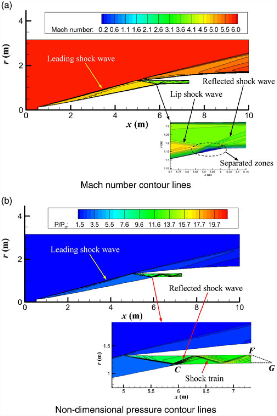
In this study, the performance parameters at the inlet exit of the basic flow model are used as the performance analysis for the basic flow model. Both the inviscid and viscous performance parameters are listed in Table 6. In this table, σ, ṁ, P e,t/P 0,t, T e/T 0, P e/P 0, and M e are all area-weighted average values on the inlet exit plane; they denote the capture mass flow coefficient, capture mass flow rate, total pressure recovery, temperature rise ratio, pressure rise ratio, and Mach number, respectively. The capture mass flow coefficient σ is evaluated as the ratio of the mass flow rate on the inlet exit plane to that on the inlet entrance plane. Moreover, both the Mach number and non-dimensional pressure contour lines under the viscous condition are shown in Fig. 22.
Comparison of inviscid and viscous performances of inlet in the axisymmetric basic flow model of the full-waverider (H = 25 km, Ma = 6.0, a = 0°)

Viscous flow fields of the basic flow model for the full-waverider vehicle under the design conditions.

Several considerable differences can be seen in the shoulder region of the isolator between the viscous case (Fig. 22) and the inviscid case (Fig. 18); the reason for these differences is the presence of the shock wave/boundary layer interactions and viscous effects of the boundary layer. From Fig. 22(a), it is observed that a small separation zone is induced by the impingement of the lip shock wave on the boundary layer of the centre body, and a corresponding reflected shock wave appears; that is, the lip shock wave does not cancel on the centre body. As a result, a well-developed shock train is established in the isolator, as shown in Fig. 22(b).
The results in Table 6 show that the viscous effects have little influence on σ and ṁ, but a great influence on P e,t/P 0,t, T e/T 0, P e/P 0, and M e. The value of σ under the viscous condition is 0.9727, and it decreases by only 2.5% in comparison to the corresponding value under the inviscid condition. This indicates that even when viscous effects are considered, the shock-on-lip condition is satisfied for the basic flow model. Furthermore, when viscous effects are considered, the T e/T 0 and P e/P 0 ratios increase by 32.4% and 27.4%, respectively; and the values of P e,t/P 0,t and M e decrease by 30.6% and 15.3%, respectively. It can be seen that the viscosity has a great effect on the performance of the total pressure recovery. This is because the viscous boundary layer causes the shock train in the inner passage of the inlet, and the shock train will seriously reduce the total pressure recovery of the inlet of the basic flow model.
4.4 Performance analysis and viscous effects on the full-waverider vehicle
Figures 20(c), 20(d) and 23 show the viscous flow fields on the inlet lip and base planes and those on the axial planes of the full-waverider vehicle under the design conditions, respectively. Similar to the above invsicid analysis, a comparison of the theoretical design and predicted shock wave locations are also shown in Figs. 20(c), 20(d) and 23, and the theoretical design shock wave locations are represented by the dashed lines in these figures. The performance parameters of the full-waverider vehicle are listed in Table 7. In Table 7, C L, C D, L/D, and C mz are the lift coefficient, drag coefficient, lift-to-drag ratio, and pitching moment coefficient, respectively, and they are used as the aerodynamic force performance parameters of the entire vehicle. In addition, σ, ṁ, P e,t/P 0,t, T e/T 0, P e/P 0, and M e are the area-weighted average values on the inlet exit plane, and they used as the inlet performance parameters.
Viscous non-dimensional pressure contour lines on axial planes of the full-waverider vehicle under the design conditions.

Comparison of inviscid and viscous performances of the full-waverider (H = 25 km, Ma = 6.0, a = 0°)

From Figs. 23 and 21, several considerable differences can be observed in the shoulder region of the isolator between the viscous case [Figs. 23(a) and 23(b)] and the inviscid case [Fig. 21(a) and 21(b)]; the reason for these differences is the presence of the shock wave/boundary layer interactions and viscous effects of the boundary layer. From Figs. 23(a) and 23(b), it is seen that the lip shock wave does not cancel on the shoulder (i.e. point D 1 in Fig. 23(a) and point D 2 in Fig. 23(b)], and a reflected shock wave appears. Thus, a well-developed shock train is established in the isolator.
On the inlet lip plane, base plane, and four axial planes as shown in Figs. 20(c), 23(d) and 23, owing to the presence of the boundary layer, the shock wave locations predicted by the numerical simulation deviate slightly from the locations of the theoretical design when the viscous effects is considered. Moreover, as shown in Figs. 20(c) and 20(d), viscous effects cause leakage of the high-pressure air from the lower surface to the upper surface, on both the inlet lip plane and the base plane.
The results in Table 7 show that the viscous effects have little impact on C L, σ, and ṁ, but great impact on C D, L/D, C mz, P e,t/P 0,t, T e/T 0, P e/P 0, and M e. The value of σ under the viscous condition is 0.9362, and it decreases by only 3.2% in comparison to the corresponding value under the inviscid condition. This indicates that even when viscous effects are considered, the shock-on-lip condition is well satisfied for the full-waverider vehicle. Furthermore, when viscous effects are considered, the values of C D, T e/T 0, and P e/P 0, increase by 91.1%, 37.2%, and 36.1%, respectively; and L/D, P e,t/P 0,t, and M e, decrease by 43.0%, 42.9%, and, 18.9%, respectively. It can be seen that the viscosity has a great effect on the performance of the total pressure recovery. This is because the viscous boundary layer causes the shock train in the inner passage of the inlet, and the shock train will seriously reduce the total pressure recovery of the inlet of the full-waverider vehicle.
5.0 CONCLUSIONS
This paper developed an upgraded airframe/inlet integration design method for the air-breathing hypersonic waverider vehicle. Numerical methods were employed to validate the applicability of this upgraded design concept to an aerodynamic configuration. Moreover, performance analyses and viscous effects of both the upgraded basic flow model and the upgraded full-waverider vehicle were numerically predicted.
1. The upgraded basic flow model derived from an axisymmetric shock wave can overcome the design limitations of the basic flow model derived from an axisymmetric generating body, and it can thus extend the design freedom of the full-waverider vehicle.
2. The inviscid numerical simulation results for the basic flow model validate the design method of the upgraded basic flow model derived from an axisymmetric basic shock wave.
3. The inviscid numerical simulation results for the full-waverider vehicle indicate that not only the forebody of the vehicle can ride on the leading-edge shock wave (i.e., forebody waverider), but also the afterbody of the vehicle can ride on the leading-edge shock wave (i.e., afterbody waverider); in other words, the vehicle is a full-waverider. This validates the design concept and design procedure of the upgraded full-waverider vehicle.
4. The shock-on-lip condition is satisfied well for both the upgraded basic flow model and the upgraded full-waverider vehicle under the design flight condition even when viscous effects are considered, thus enabling the inlet to efficiently capture the precompression air flow.
5. The results obtained from this study demonstrate that the upgraded full-waverider approach is effective in designing the airframe/inlet integrated waverider vehicle.
6.0 ACKNOWLEDGEMENTS
The authors would like to express their gratitude for the financial support provided by the National Natural Science Foundation of China (grant number 11702322) and the Natural Science Foundation of Hunan Province of China (grant number 2018JJ3589). The authors are also grateful to the reviewers for their extremely constructive comments.
Conflict of interest statement
The authors declare that they have no conflict of interest.