


Impact Statement
Detecting supraglacial lakes (SGLs) on Antarctica’s ice sheets is important for glacier mass balance modeling and sea level rise projections. The presence of SGLs can have a negative influence on ice shelf stability by inducing hydrofracture and causing flexure, and reduces firn air content and surface albedo, which facilitates the formation of new surface water bodies. Due to the vastness and remoteness of the area, information about SGLs is commonly derived in automated workflows from large amounts of multispectral satellite imagery. While there are several established mapping approaches, the advent of DL for image segmentation offers a new methodology that enables the inclusion of spatial information into formerly pixel-wise image classification workflows. Our newly trained U-net DL model outperforms a traditional random forest-based mapping approach and maps by averaging the largest lake area in a relative comparison with five conventional methods. Although potential improvements still remain, once trained, the method is easily applicable on larger scales and thus lays the foundation for comprehensive circum-Antarctic SGL mapping efforts that can improve glacier mass balance modeling and sea level rise estimations in the context of global warming.
1. Introduction
Surface meltwater in Antarctica has been increasingly discussed as a determining factor in ice shelf instability and hence global sea level rise due to global warming (Lai et al., Reference Lai, Kingslake, Wearing, Chen, Gentine, Li, Spergel and Van Wessem2020; Gilbert and Kittel, Reference Gilbert and Kittel2021; Van Wessem et al., Reference Van Wessem, Den Broeke, Wouters and Lhermitte2023; De Roda Husman et al., Reference De Roda Husman, Lhermitte, Bolibar, Izeboud, Hu, Shukla, Van Der Meer, Long and Wouters2024). Meltwater ponding within crevasses can promote downward crack propagation, potentially leading to hydrofracture (Bell et al., Reference Bell, Banwell, Trusel and Kingslake2018; Robel and Banwell, Reference Robel and Banwell2019; Lai et al., Reference Lai, Kingslake, Wearing, Chen, Gentine, Li, Spergel and Van Wessem2020). In addition, the filling and drainage of melt ponds, together with the redistribution of meltwater across the ice shelf, can induce flexure and thereby weaken the structural integrity of the shelf (Banwell et al., Reference Banwell, Willis, Macdonald, Goodsell and MacAyeal2019). Both processes may result in through-ice fractures that can ultimately trigger the disintegration of entire ice shelves, as observed for the Larsen B Ice Shelf collapse (Banwell et al., Reference Banwell, MacAyeal and Sergienko2013). Meanwhile, refreezing meltwater promotes the formation of ice lenses and firn densification. These processes inhibit water percolation and storage, increase surface runoff, and thereby enhance the formation of new surface water bodies (Hubbard et al., Reference Hubbard, Luckman, Ashmore, Bevan, Kulessa, Kuipers Munneke, Philippe, Jansen, Booth, Sevestre, Tison, O’Leary and Rutt2016; Machguth et al., Reference Machguth, MacFerrin, Van As, Box, Charalampidis, Colgan, Fausto, Meijer, Mosley-Thompson and Van De Wal2016; Buzzard et al., Reference Buzzard, Feltham and Flocco2018). This, in turn, has direct implications for the energy balance of ice shelves, as the resulting reduction in surface albedo further amplifies melt rates (Arthur et al., Reference Arthur, Stokes, Jamieson, Carr and Leeson2020). In Antarctica, only a few studies have observed a coupling between surface meltwater systems and the subglacial hydrological system of grounded ice, for example, via moulins (Bell et al., Reference Bell, Banwell, Trusel and Kingslake2018; Tuckett et al., Reference Tuckett, Ely, Sole, Livingstone, Davison, Van Wessem and Howard2019). However, observations from Greenland have shown that increased meltwater input from supraglacial lakes (SGLs) into the subglacial drainage system can enhance basal sliding and accelerate glacier flow (Tedesco et al., Reference Tedesco, Willis, Hoffman, Banwell, Alexander and Arnold2013; Wehrlé et al., Reference Wehrlé, Lüthi, Kneib-Walter, Nap, Rousseau, Jouvet and Walter2026). A similar scenario may become possible in Antarctica with the continued inland migration of SGLs (Dirscherl et al., Reference Dirscherl, Dietz and Kuenzer2021b). In combination with the reduced buttressing effect of already disintegrated ice shelves, this could further accelerate ice flow and exacerbate mass loss on connected glaciers (Royston and Gudmundsson, Reference Royston and Gudmundsson2016; Rott et al., Reference Rott, Abdel Jaber, Wuite, Scheiblauer, Floricioiu, Van Wessem, Nagler, Miranda and Van Den Broeke2018). Projections suggest a doubling of current surface melt rates in Antarctica by 2050 (Trusel et al., Reference Trusel, Frey, Das, Karnauskas, Kuipers Munneke, Van Meijgaard and Van Den Broeke2015), with likely implications for global sea level rise.
The spatial extent, remoteness, and inaccessibility make it difficult to quantify surface meltwater extent and volume using in-situ measurements, particularly on Antarctica’s vast ice sheets. Therefore, the use of spaceborne remote sensing data to map meltwater surface features such as lakes, streams, and water-saturated firn and snow (“slush”) has become increasingly important in recent years (e.g., Stokes et al., Reference Stokes, Sanderson, Miles, Jamieson and Leeson2019; Dirscherl et al., Reference Dirscherl, Dietz, Kneisel and Kuenzer2020; Moussavi et al., Reference Moussavi, Pope, Halberstadt, Trusel, Cioffi and Abdalati2020b; Corr et al., Reference Corr, Leeson, McMillan, Zhang and Barnes2022; Dell et al., Reference Dell, Willis, Arnold, Banwell and De Roda Husman2024). Spaceborne remote sensing provides spatially continuous, large-scale measurements at resolutions on the order of tens of meters. In polar regions, the usual revisit frequency of several days is improved by overlapping swaths and can be further enhanced by combining different sensors. In addition, the long-term continuity of satellite missions allows the analysis of multiyear time series. Therefore, a variety of approaches have been developed to derive the extent and volume of surface meltwater in polar regions. Studies relying on multispectral satellite data often use a threshold-based SGL detection approach. Earlier studies mostly used single-band reflectance thresholds (Sneed and Hamilton, Reference Sneed and Hamilton2007; Liang et al., Reference Liang, Colgan, Lv, Steffen, Abdalati, Stroeve, Gallaher and Bayou2012; Moussavi et al., Reference Moussavi, Abdalati, Pope, Scambos, Tedesco, MacFerrin and Grigsby2016; Williamson et al., Reference Williamson, Willis, Arnold and Banwell2018) or the ratio between the visible blue and red channels (Box and Ski, Reference Box and Ski2007; Pope et al., Reference Pope, Scambos, Moussavi, Tedesco, Willis, Shean and Grigsby2016; Banwell, Reference Banwell2017). Other thresholding approaches depend on one (Morriss et al., Reference Morriss, Hawley, Chipman, Andrews, Catania, Hoffman, Lüthi and Neumann2013; Yang and Smith, Reference Yang and Smith2013; Stokes et al., Reference Stokes, Sanderson, Miles, Jamieson and Leeson2019) or multiple (Burton-Johnson et al., Reference Burton-Johnson, Black, Fretwell and Kaluza-Gilbert2016) spectral indices such as normalized differences between two spectral channels. Recent studies commonly utilize the approach developed by Moussavi et al. (Reference Moussavi, Pope, Halberstadt, Trusel, Cioffi and Abdalati2020b), which combines the normalized difference water index (NDWI), the normalized difference snow index (NDSI), and various thresholds on single spectral bands. This method exploits the light attenuation of SGLs and the resulting reflectance differences in the green and near-infrared, and blue and red spectral bands, respectively. Using a physical model, it is also possible to calculate lake depth and volume. This approach has been applied with high classification accuracy to ice shelves in West Antarctica and the Antarctic Peninsula (Corr et al., Reference Corr, Leeson, McMillan, Zhang and Barnes2022), East Antarctica (Spergel et al., Reference Spergel, Kingslake, Creyts, Van Wessem and Fricker2021; Tuckett et al., Reference Tuckett, Ely, Sole, Lea, Livingstone, Jones and Van Wessem2021; Arthur et al., Reference Arthur, Stokes, Jamieson, Rachel Carr, Leeson and Verjans2022; Trusel et al., Reference Trusel, Pan and Moussavi2022), and the entire continent (Shen et al., Reference Shen, Ke, Li, Cai, Xiao and Li2025). However, because optical data are prone to misclassification in the presence of slush, rocks, clouds, and shadows, careful post-processing of classification results is required (Corr et al., Reference Corr, Leeson, McMillan, Zhang and Barnes2022). This, along with limited transferability of static thresholds to other regions, makes upscaling this method to larger spatial scales challenging (Tuckett et al., Reference Tuckett, Ely, Sole, Lea, Livingstone, Jones and Van Wessem2021; Dell et al., Reference Dell, Banwell, Willis, Arnold, Halberstadt, Chudley and Pritchard2022).
This problem has recently been addressed by machine learning-based image classification and segmentation approaches. For the first time, Dirscherl et al. (Reference Dirscherl, Dietz, Kneisel and Kuenzer2020) used a Random Forest classifier (RF) and demonstrated its usefulness for SGL mapping from Sentinel-1 data over a variety of regions in Antarctica. Hu et al. (Reference Hu, Huang, Chi, Cheng, Wei, Chen, Xu, Qi, Xu and Zheng2022) trained an RF with Sentinel-2-derived NDWI and textural features to map SGLs over the entire Greenland ice sheet. The good overall accuracy of the results over such a large area indicates good transferability of the method, although an application in Antarctica is still pending. The issue of distinguishing slush from ponded water in Landsat data is addressed by Dell et al. (Reference Dell, Banwell, Willis, Arnold, Halberstadt, Chudley and Pritchard2022, Reference Dell, Willis, Arnold, Banwell and De Roda Husman2024), who trained an RF to separate these two spectrally similar classes in Antarctica.
While threshold-based and RF approaches heavily rely on the spectral information of optical datasets, some studies have also explored using spatial features by employing convolutional neural networks for image segmentation, more specifically modified versions of the original U-net by Ronneberger et al. (Reference Ronneberger, Fischer, Brox, Navab, Hornegger, Wells and Frangi2015). For multispectral data, this neural network was applied for the first time by Lutz et al. (Reference Lutz, Bahrami and Braun2023) to detect SGLs in Sentinel-2 imagery over two glaciers in Greenland. The U-net’s focus on spatial information enabled the study to limit the provided spectral information for model training to only three bands (red, blue, and green) and nonetheless achieved a high classification accuracy. Meanwhile, the full spectral information of Sentinel-2 was used by Niu et al. (Reference Niu, Tang, Yang, Zhang, Zheng and Wang2023) for SGL mapping in six consecutive melting seasons over the Amery ice shelf in Antarctica. Different artificial neural network approaches were compared, with an attention-based U-net achieving the best results. Moreover, studies that attempted mapping SGLs from synthetic aperture radar (SAR) backscatter data have shown that a U-net is well suited to this task even on data with low spectral variety (Chen, Reference Chen2021; Dirscherl et al., Reference Dirscherl, Dietz, Kneisel and Kuenzer2021a; Jiang et al., Reference Jiang, Li, Zhang, Marinsek, Hong and Wu2022). This indicates that including spatial features into the modeling reduces the dependence on spectral features and might reduce the amount of data needed in large-scale mapping efforts based on multispectral data. The combination of spectral information and spatial context makes the U-net an appealing classifier for optical data, where other classification approaches have difficulties in discriminating spectrally similar classes such as slush from SGLs. If provided with a wide variety of training scenes containing different surface features, this approach has the potential for pan-Antarctic SGL mapping. Therefore, we investigate how much a deep neural network enhances SGL mapping accuracy compared to traditional and machine learning (ML) methods.
In this article, we present an automated mapping workflow that uses a U-net to detect SGLs in multispectral Sentinel-2 data. In particular, we build on the work by Dirscherl et al. to advance their SGL mapping approach for optical data (Dirscherl et al., Reference Dirscherl, Dietz, Kneisel and Kuenzer2020) by adapting and evaluating a U-net architecture that was originally implemented for the same purpose for SAR data (Dirscherl et al., Reference Dirscherl, Dietz, Kneisel and Kuenzer2021a, Reference Dirscherl, Dietz and Kuenzer2021b). As demonstrated in this work, this can potentially reduce the amount of required input data and thus streamline the processing for large-scale mapping efforts. Currently, for multispectral data, 18 features (spectral bands plus derived indices) are required to train an RF model (Dirscherl et al., Reference Dirscherl, Dietz, Kneisel and Kuenzer2020). We argue that the U-net’s awareness of the spatial context will reduce the amount of spectral information required. We also aim to explore potential improvements of our approach in discriminating spectrally similar classes, for example, shallow lakes and slush, and contextual features, such as ice cover, lake edges, or cloud shadows. To this end, we (i) generate high-precision training and validation labels of SGLs on Sentinel-2 imagery of a wide selection of Antarctica’s marginal ice shelves and glaciers; (ii) train and evaluate different configurations of a Deep Learning (DL) model to detect SGLs in Sentinel-2 data; (iii) comprehensively compare our results with an ML approach by Dirscherl et al. (Reference Dirscherl, Dietz, Kneisel and Kuenzer2020) using manually labeled validation data; and (iv) compare the DL-based classification results to established SGL mapping datasets.
This article is organized as follows: Section 2 describes the datasets, training and test sites, model architecture, validation approaches, and comparison schemes used. Section 3 presents the results of the accuracy evaluation of the DL approach in direct comparison to its RF predecessor, as well as other SGL mapping products. Section 4 discusses the results in terms of improvements and drawbacks of the proposed approach compared to the original and other products. Section 5 summarizes the results and provides an outlook for future research.
2. Materials and methods
In this article, we develop a DL-based SGL detection approach for Sentinel-2 data (Figure 1). First, training and testing data are acquired, then the most suitable spectral features to detect SGLs are determined. Using these data, a U-net model is tuned, trained, and evaluated. The final model is then used for large-scale inference of SGLs in Antarctica. The materials and methods used in this workflow will be presented in detail below.
Conceptual workflow of the proposed Sentinel-2-based supraglacial lake detection approach. Figure contains elements from https://www.freepik.com/.

Figure 1. Long description
The flowchart is organized into four vertical columns, each with a dark blue header. A vertical label on the far left reads Sentinel-2.
* Stage 1: data acquisition. This column shows an outline of Antarctica with several red and blue square frames placed along its coastline, representing satellite image tiles.
* Stage 2: feature selection. An arrow points from the first stage to a stack of five semi-transparent colored planes (green, red, purple, and gray), representing different spectral bands or data layers.
* Stage 3: model training and evaluation. An arrow points to a U-Net architecture diagram, showing a downward and upward path of blue blocks connected by lines, with a neural network icon at the top. A feedback arrow points from the bottom of this model back to the feature selection stage.
* Stage 4: inference and post-proc. A final arrow points to a square image showing a high-resolution classification map with pink and white regions, representing detected supraglacial lakes.
2.1. Datasets, training, and testing sites
To derive SGLs, we used data from the Sentinel-2 mission (European Space Agency, 2022). This constellation of three satellites carries a passive Multispectral Instrument (MSI) that records reflectance values in 13 spectral bands at a spatial resolution of up to 10 meters. Sentinel-2 data have been available since 2015 with a revisit time of 5 days, which is effectively higher at the poles due to overlapping swaths. For this study, we use Level-1C Top-of-Atmosphere reflectance data (European Space Agency, 2022).
For model training and testing, we selected a variety of testing sites distributed across Antarctica to reflect regional variability. We selected sites where SGL occurrence had been reported before in the literature. We aimed for scenes acquired during the melting season in austral summer (November to March) where SGL numbers and extents peak. However, we had to prioritize scenes with an abundance of lakes, so the selected data covered the months of December to February, with a strong focus on January. For the same reason, most of the training and testing data are from the strong melting seasons of 2019/2020 and 2020/2021, but the years 2017, 2018, 2023, and 2024 were also covered. Furthermore, the training and testing data reflect a variety of environmental settings, including diverse surface features next to lakes, such as slush, blue ice, rock outcrops, clouds and cloud shadows, moraines, and crevasses (Figure 2). It was also ensured that the large variety of SGL types was reflected, such as deep and shallow lakes, ice cover, oval and elongated lakes, as well as ice.
Visual examples of various surface features included in the train and test datasets. (a) Oval lakes at Roi Baudouin, (b) shallow lakes at Roi Baudouin, (c) lake among crevasse fields at Shirase Glacier, (d) thin ice cover at Amundsen, (e) a thick ice lid at Amery, (f) slush at Riiser, (g) blue ice at Nivlisen, (h) lakes under clouds at George VI, (i) dark clouds over Amundsen, and (j) thin streams at Amery. Background: Copernicus Sentinel-2 Data.

Figure 2. Long description
The figure consists of ten satellite image panels arranged in two rows. Each panel includes a black scale bar in the bottom-left corner.
Top Row:
* Panel a: A single, elongated blue oval lake surrounded by white ice. Scale bar is 1.5 k m.
* Panel b: Two narrow, irregular shallow lakes with dark outlines on a light blue ice surface. Scale bar is 0.5 k m.
* Panel c: Dark blue irregular lake shapes situated within a heavily textured, white and grey crevasse field. Scale bar is 0.5 k m.
* Panel d: A large, elongated blue lake with a thin, translucent white ice cover visible on its surface. Scale bar is 0.5 k m.
* Panel e: Several elongated blue lakes, one featuring a prominent, thick grey ice lid in its center. Scale bar is 1 k m.
Bottom Row:
* Panel f: A pale, yellowish-white surface representing slush with faint green-blue streaks. Scale bar is 0.5 k m.
* Panel g: A vast expanse of smooth, bright blue ice with mottled white patches. Scale bar is 4 k m.
* Panel h: Numerous small, dark-outlined horizontal lake streaks partially obscured by a grey cloud layer. Scale bar is 4 k m.
* Panel i: High-contrast dark and bright white clouds obscuring the ground surface. Scale bar is 1 k m.
* Panel j: Three thin, linear blue streams arranged in a diagonal line across a white ice field. Scale bar is 0.3 k m.
For model training, 16 Sentinel-2 scenes were acquired, in which 33 training areas were defined. The performance of the model was validated on 8 Sentinel-2 scenes containing 16 testing sites (Figure 3 and Supplementary Table S1). The cloud cover percentage of the training scenes ranges from 0 to 94.9, while the mean sun elevation angle varies between 20.2 and 36.1 degrees. In the testing scenes, the cloud cover percentages ranges from 0 to 54.6 and the mean sun elevation angle from 26.8 to 38.3 degrees (Supplementary Table S1).
Locations of the training and testing sites. The map is displayed in Polar Stereographic projection. Base maps provided by the Antarctic Digital Database (https://add.scar.org/).

Figure 3. Long description
A Polar Stereographic map of Antarctica with a coordinate grid. Training sites are marked with pink squares, test sites with green squares, and combined sites with yellow dots.
* In the West, the Antarctic Peninsula contains Larsen C (test), Wilkins (training), and George V I (combined training and test).
* Moving clockwise to the North, sites include Riiser-Larsen (training), Nivlisen (combined), and Roi Baudouin (test).
* In the Northeast and East, sites include Shirase (training), Enderby (test), Kemp (training), Amery (training), and Shackleton (training).
* In the Southeast, sites include Moscow (test) and Mawson (training).
* In the Southwest, sites include Hull (test), Pine Island Bay (training and test), and Abbott (training and test).
A legend in the bottom-left corner defines the symbols: pink square for Training site, green square for Test site, and yellow dot for Training and test site.
Additionally, the 90–m TanDEM-X PolarDEM digital elevation model (DEM) was used to mask out steep slopes (> 5%), where lake formation is highly unlikely, and high altitudes during post-processing (Wessel et al., Reference Wessel, Huber, Wohlfart, Bertram, Osterkamp, Marschalk, Gruber, Reuß, Abdullahi, Georg and Roth2021). To mask out areas seaward of the Antarctic coastline, we use the IceLines product to determine the ice shelf front positions in coastal areas (Baumhoer et al., Reference Baumhoer, Dietz, Heidler and Kuenzer2023). To compare the performance of the proposed U-net-based mapping approach, we use existing SGL maps generated by Dirscherl et al. (Reference Dirscherl, Dietz, Kneisel and Kuenzer2020) where available or otherwise created them ourselves using the original RF-based workflow.
We selected five SGL datasets that use optical satellite imagery to map supraglacial lakes in Antarctica (Table 1), which we compared to the mapping results of our proposed approach (see Section 2.3). The dataset by Stokes et al. (Reference Stokes, Sanderson, Miles, Jamieson and Leeson2019) uses both Landsat 8 and Sentinel-2 data to map SGLs on the margins of the East Antarctic ice sheet (EAIS) for January 2017. Lakes were automatically detected by thresholding the NDWI, which calculates the normalized difference of the green and near-infrared (NIR) spectral bands. The SGL dataset by Moussavi et al. (Reference Moussavi, Pope, Halberstadt, Trusel, Cioffi and Abdalati2020b) covers 20 regions across Antarctica and the years 2013–2020. It is derived from Landsat 8 data by thresholding an NDWI variant that uses the blue and red spectral channels, as well as differences between green and red, and blue and green, respectively, to identify potential lake areas. Further thresholding using the NDSI (green and short-wave infrared bands) and a ratio between brightness temperature and the blue spectral band masks out clouds, rocks, and seawater. It is noteworthy that that even though the original mapping approach combines Landsat 8 and Sentinel-2 data (Moussavi et al., Reference Moussavi, Pope, Halberstadt, Trusel, Cioffi and Abdalati2020b), the published dataset itself is based only on Landsat 8 (Moussavi et al., Reference Moussavi, Abdalati, Halberstadt, Pope and Trusel2020a). This approach and its thresholds were adapted and modified by Corr et al. (Reference Corr, Leeson, McMillan, Zhang and Barnes2022) to include both above-mentioned NDWI variants. The resulting dataset covers the West Antarctic Ice Sheet (WAIS) and Antarctic Peninsula (API) for January 2017 and, furthermore, discriminates between lakes and channels. Finally, we included the SGL and slush dataset by Dell et al. (Reference Dell, Banwell, Willis, Arnold, Halberstadt, Chudley and Pritchard2022, Reference Dell, Willis, Arnold, Banwell and De Roda Husman2024), which covers 57 ice shelves across Antarctica between 2013 and 2021 and is derived from Landsat 8 data. The method considers areas above a fixed NDWI (blue and red channels) threshold, which are then clustered in an unsupervised classification scheme. Among others, the classes “ponded water” and “slush” were determined, and a sample of pixels from each class was used to train an RF classifier. Finally, we used the method described by Dirscherl et al. (Reference Dirscherl, Dietz, Kneisel and Kuenzer2020) to create SGL maps for the accuracy assessment (Section 2.2.4) and the relative dataset comparison (Section 2.3). In this approach, an RF classifier is trained on 18 spectral features such as spectral bands and indices, including both variants of the NDWI to detect SGLs.
SGL datasets and their characteristics used in the relative comparison scheme

Table 1. Long description
The table consists of four columns and six data rows.
1. Dataset: U-net. Spatial coverage: A P I, E A I S, W A I S. Method: U-net. Sensors: Sentinel-2.
2. Dataset: Stokes et al. 2019. Spatial coverage: E A I S. Method: N D W I thresholding. Sensors: Landsat 8, Sentinel-2.
3. Dataset: Moussavi et al. 2020a. Spatial coverage: A P I, E A I S, W A I S. Method: N D W I / N D S I thresholding. Sensors: Landsat 8, Sentinel-2.
4. Dataset: Dirscherl et al. 2020. Spatial coverage: A P I, E A I S, W A I S. Method: Random Forests. Sensors: Sentinel-2.
5. Dataset: Corr et al. 2022. Spatial coverage: W A I S, A P I. Method: Modified Moussavi et al. 2020. Sensors: Landsat 8, Sentinel-2.
6. Dataset: Dell et al. 2024. Spatial coverage: A P I, E A I S, W A I S. Method: N D W I thresholding, Random Forests. Sensors: Landsat 8.
Note: A P I refers to Antarctic Peninsula, E A I S refers to East Antarctic Ice Sheet, and W A I S refers to West Antarctic Ice Sheet.
Note. The column spatial coverage indicates the Antarctic region (partially) covered by the dataset: API, Antarctic Peninsula; EAIS, East Antarctic Ice Sheet; WAIS, West Antarctic Ice Sheet.
Another SGL dataset worth mentioning is that by Arthur et al. (Reference Arthur, Stokes, Jamieson, Rachel Carr, Leeson and Verjans2022). It covers the EAIS between 2014 and 2020, and is derived from Landsat 8 data. However, since the classification workflow closely follows that by Moussavi et al. (Reference Moussavi, Pope, Halberstadt, Trusel, Cioffi and Abdalati2020b), we did not include this.
2.2. Supraglacial lake mapping
2.2.1. Label generation and data preprocessing
There is no universally accepted definition of a “supraglacial lake” in the existing literature, to our knowledge. As a basis for this study, we adopt the classification scheme of Dell et al. (Reference Dell, Banwell, Willis, Arnold, Halberstadt, Chudley and Pritchard2022) who distinguish stored surface meltwater on Antarctic ice shelves as either ponded water (i.e., lakes) or meltwater retained within firn pore spaces. This distinction implicitly separates supraglacial lakes from other surface hydrological features such as streams and slush. Building on this framework, we introduce several modifications and caveats to establish consistent training labels for the target class “supraglacial lake” across different scenes and geographical settings.
First, we only consider lakes that form on ice (Supplementary Table S2 [a]). For some ice-marginal lakes, it is not possible to determine unequivocally whether the water body is situated on bedrock or ice; however, if the lake is in direct contact with the ice surface, we classify it as an SGL (Supplementary Table S2 [p]). Second, we consider the morphology of water bodies within supraglacial hydrological networks. Narrow channels connecting wider ponded areas are excluded (Supplementary Table S2 [g]), whereas broad, stream-like features are included, as the distinction between elongated lakes and wide streams is often arbitrary and such features can retain substantial volumes of meltwater over extended periods (Supplementary Table S2 [h]). Third, we only classify lake areas that are visible in the imagery. This also includes lakes that can be identified through spatial context, such as lakes that are faintly visible beneath thin cloud cover (Supplementary Table S2 [o]) or ice (Supplementary Table S2 [b]–[d]). We argue that the spatial awareness of the tested segmentation model facilitates the detection of such features.
Based on these considerations, a concise rule set was developed in which labeling guidelines for a variety of scenarios (e.g., ice cover, minimum lake size, streams, lakes under clouds, etc.) were formulated. These rules are documented with examples in Supplementary Table S2. In experiments, we found that a reduced number of consistent high-precision labels generated following this rule set resulted in significantly higher classification accuracies than an increased amount of less consistent training data, for example, generated through automated thresholding.
Using this ruleset, we generated fully segmented training and testing scenes by manually digitizing SGLs in the selected training and testing regions. SGL areas, as per our definition above, were labeled “1” (the target class) and everything else “0”. Next, the acquired Sentinel-2 L1C data were atmospherically corrected to L2A Bottom-Of-Atmosphere (BOA) reflectance using the Sen2Cor processor (Pignatale, Reference Pignatale2022). Digital numbers (DNs) were converted to reflectance values using the appropriate scaling factors and offsets for the respective processing baseline of the product. Missing no data values (DN = 0) inside the image acquisition strip of the scene were spatially interpolated. For both the training and testing scenes, image stacks were generated that contained the spectral bands in the visible green and red (Sentinel-2 bands 3 and 4), as well as the Soil/Water Index (SWI) (Dirscherl et al., Reference Dirscherl, Dietz, Kneisel and Kuenzer2020) and the Automated Water Extraction Index (AWEInsh [Feyisa et al., Reference Feyisa, Meilby, Fensholt and Proud2014]) (Table 2). These bands and indices were selected as they were previously found to have high predictive power for SGL detection (Dirscherl et al., Reference Dirscherl, Dietz, Kneisel and Kuenzer2020) and our empirical experiments showed that the AWEInsh in particular reduced misclassifications in areas with topographic shadows (Supplementary Figure S1), while the SWI is useful for the discrimination of rocks and moraines from water bodies. The shortwave infrared bands (SWIR1 and SWIR2) were resampled for this purpose to match the 10 m resolution of bands 3 and 4.
Spectral features included in the training of the Sentinel-2-based SGL detection model

Table 2. Long description
The table consists of four rows of data under the headers No., Band forward slash index, Description forward slash formula, and Reference.
* Row 1: Number 1. Band B 0 3. Description: Visible green (560 nm). Reference: s e n t i w i k i dot copernicus dot e u forward slash web forward slash s 2 minus mission.
* Row 2: Number 2. Band B 0 4. Description: Visible red (665 nm). Reference: Same as Row 1.
* Row 3: Number 3. Band S W I. Formula: (Blue minus S W I R 1) forward slash (Blue plus S W I R 1). Reference: Dirscherl et al. 2020.
* Row 4: Number 4. Band A W E I sub n s h. Formula: 4 times (Green minus S W I R 1) minus (0.25 times N I R) plus (2.75 times S W I R 2). Reference: Feyisa et al. 2014.
The training data consists of binary label masks and corresponding imagery containing information on the spectral bands and indices. This dataset was used for model training and internal validation to iteratively optimize the model parameters.
First, the training data were tiled into 480 × 480 pixel tiles with an overlap of 100 pixels that could be fed into the model training pipeline. The resulting stack of 658 tiles was subdivided depending on the number of labeled lakes visible within a tile, that is, in stacks containing no lakes, few lakes, and many lakes. The threshold between few and many lakes was drawn at the 80th percentile, that is, tiles with an amount of more than 15,041 lake pixels were considered “lake-rich.” To increase the number of training samples and address the imbalance of the classes “lake” and “no lake,” we applied an augmentation strategy to the training data (Dirscherl et al., Reference Dirscherl, Dietz, Kneisel and Kuenzer2021a). Tiles containing lakes were flipped, shifted, and rotated to various degrees, with tiles containing numerous lakes being augmented 12 times and tiles with fewer lakes 8 times. Additionally, tiles containing particularly difficult surface features such as clouds and dark topographic shadows were augmented 12 times regardless of whether they contained any lakes. The resulting tiles, along with a 3% random selection of lake-less tiles, comprised the final stack of training data containing a total of 3,420 tiles. For each of the four bands of the training imagery, we calculated statistics such as the minimum, maximum, mean, and standard deviation across all tiles. Then, each tile and band was normalized using z-score normalization. The final training data were then subdivided into 80% training data and 20% validation data for the internal model validation, resulting in stacks of 2,736 labels and images for training and 684 for validation. It is noteworthy that labels and imagery used in the accuracy assessment (Section 2.2.4) were not used during model training.
2.2.2. U-net model architecture and training
The aim of this article is to analyze how a deep-learning image segmentation approach can improve SGL detection.
The U-net, which has been used for image segmentation of various surface features on a variety of Earth observation datasets before, typically consists of an image encoding followed by a decoding pipeline and yields a probability map of the target class. Specifically, variants of this architecture have been used in local and regional studies for the detection of SGLs in multispectral (Lutz et al., Reference Lutz, Bahrami and Braun2023; Niu et al., Reference Niu, Tang, Yang, Zhang, Zheng and Wang2023) and SAR data (Chen, Reference Chen2021; Dirscherl et al., Reference Dirscherl, Dietz, Kneisel and Kuenzer2021a). For this study, we use the U-net architecture proposed by Dirscherl et al. (Reference Dirscherl, Dietz, Kneisel and Kuenzer2021a). It uses residual skip connections and Atrous Spatial Pyramid Pooling (ASPP) and has significantly improved SGL mapping accuracies based on Sentinel-1 SAR data before (Dirscherl et al., Reference Dirscherl, Dietz, Kneisel and Kuenzer2021a). We decided to evaluate this specific architecture because (i) we were already familiar with its code and application; (ii) we expected it to adapt well to the multispectral data during the training process based on the aforementioned studies; and (iii) our initial tests already showed good results. The only modification made to the model architecture is that the input imagery contains four layers instead of one. These spectral features comprise the ones depicted in Table 2.
The evaluated U-net architecture consists of four downsampling (encoding) and four corresponding upsampling blocks (decoding), with the deepest blocks being connected by an ASPP module (Chen et al., Reference Chen, Papandreou, Kokkinos, Murphy and Yuille2018) (Figure 4). In each downsampling block, the input layer is convoluted two times using a 3×3 kernel, while the original image size is kept by padding. Additionally, the input layer is convoluted with a 1×1 kernel and added to the previously generated convoluted layer to establish a residual connection to keep the original input information in later steps of the model. A transformation using the Leaky nonlinear Rectified Linear Unit (LeakyReLU) activation function is introduced to enable nonlinear modeling. Then, the image size is halved by applying a 2 × 2 maximum pooling operation, and 30% of neurons are dropped out to avoid overfitting. The resulting image comprises the input to the next downsampling block. This procedure is repeated until a depth of 512 layers is reached. The resulting image features are then put into an ASPP block, in which they are convoluted with dilation rates of 2, 4, 8, and 12, and the outputs are concatenated. This enhances the model’s ability to learn and model lakes of different shapes and sizes. To restore the original image size, features are then given into four upsampling blocks that mirror the convolution strategy of the downsampling blocks. Additionally, via a skip connection, each upsampled feature is concatenated with the output of the corresponding downsampling block. This enables the reconstruction of the high-resolution image information from the lower-resolution features while maintaining the abstraction level of the convoluted features. In the final upsampling block, the output image size is reconstructed with an image depth of 1 and passed into a sigmoid activation function that returns a probability map of SGL occurrence. For model training, the Adamax optimizer with an initial learning rate of 0.0001 was selected, which was reduced by a factor of 10 if the learning rate did not improve over three epochs. Learning was finished if a learning rate of 0.0000001 was reached. “Binary cross-entropy” was used as the loss function.
Architecture of the U-net model used for Sentinel-1 and Sentinel-2-based supraglacial lake detection. Modified after Dirscherl et al. (Reference Dirscherl, Dietz, Kneisel and Kuenzer2021a).

Figure 4. Long description
The flowchart illustrates a U-Net architecture. At the top-left, input data is represented by four stacked colored layers. The contracting path on the left descends through four levels, with dimensions decreasing from 480 by 480 to 30 by 30, and feature channels increasing from 4 to 512. Each level uses dark blue blocks connected by blue arrows for conv 3x3 Leaky ReLU and red arrows for max pool 2x2. At the bottom center, an A S P P block connects the contracting and expansive paths. The expansive path on the right ascends through four levels, with dimensions increasing back to 480 by 480. This path uses light blue blocks connected by green arrows for up-conv 2x2, orange arrows for dropout 0.3, and yellow arrows for concat. conv 1x1 Leaky ReLU. Horizontal grey arrows represent skip connections linking corresponding levels of the contracting and expansive paths. The final output at the top-right is a single-channel binary mask labeled 1, shown as a black and white image of lake features. A legend at the top center defines the operations: blue arrow for conv 3x3 Leaky ReLU, light blue arrow for conv 3x3, red arrow for max pool 2x2, orange arrow for dropout 0.3, green arrow for up-conv 2x2, grey line for skip connection, yellow arrow for concat. conv 1x1 Leaky ReLU, light green arrow for conv 1x1 sigmoid, and a red circle icon for conv 1x1 add Leaky ReLU.
The model was trained for 50 epochs, but convergence in the internal model validation was reached much earlier (Figure 5). The best model run was achieved at epoch 16 at a loss rate of 0.06 and an accuracy of 0.97. Since there was some fluctuation at later epochs, the model from epoch 25 was selected for validation and inference, as the model loss and accuracy fully stabilized at 0.06 and 0.97, respectively.
Internal accuracy and loss rate of the trained U-net model.

Figure 5. Long description
A two-panel figure titled Learning curve.
Left panel: The x-axis is labeled Epochs ranging from 0 to 50. The y-axis is labeled log_acc ranging from 0.88 to 0.98. Two lines are plotted. The blue line represents accuracy, showing a steep logarithmic increase from 0.89 at epoch 0 to a plateau of approximately 0.978 starting around epoch 20. The orange line represents val_accuracy, which shows a more volatile increase, peaking near epoch 18 and stabilizing slightly below the training accuracy at approximately 0.976.
Right panel: The x-axis is labeled Epochs ranging from 0 to 50. The y-axis is labeled log_loss ranging from 0.05 to 0.25. The blue line represents loss, showing a sharp asymptotic decrease from 0.26 at epoch 0 to a stable floor of 0.05 by epoch 20. The orange line represents val_loss, which decreases with fluctuations. A red X marks the best model at approximately epoch 15 with a loss of 0.06. A green X marks the selected model at epoch 25 with a loss of approximately 0.063. Both loss curves plateau after epoch 25.
2.2.3. Post-processing
The output of each U-net run is a 480 × 480 pixel probability map of SGL occurrence. All tiles of a scene are reassembled to reconstruct the original images x- and y-dimensions. For overlapping areas introduced during the tiling process, the mean probability is calculated. Next, topographic masking of areas with slopes steeper than 5% and altitudes higher than 1,500 m was applied using the TanDEM-X PolarDEM. Furthermore, areas seaward of the coastline as derived by the IceLines product (Baumhoer et al., Reference Baumhoer, Dietz, Heidler and Kuenzer2023) were excluded. Next, thresholds of 90% and 99% probability were applied to generate binary lake/no-lake maps. Lake areas smaller than three pixels (~300m2) were sieved out to reduce image noise. It is common practice in other SGL mapping studies (Stokes et al., Reference Stokes, Sanderson, Miles, Jamieson and Leeson2019; Dirscherl et al., Reference Dirscherl, Dietz, Kneisel and Kuenzer2020, Reference Dirscherl, Dietz, Kneisel and Kuenzer2021a; Moussavi et al., Reference Moussavi, Pope, Halberstadt, Trusel, Cioffi and Abdalati2020b; Corr et al., Reference Corr, Leeson, McMillan, Zhang and Barnes2022) to filter out small lakes with sizes equal and lower than 2–45 pixels, depending on the spatial resolution of the input data. In a systematic assessment, Stokes et al. (Reference Stokes, Sanderson, Miles, Jamieson and Leeson2019) report the lake area omitted by filtering to be insubstantial compared to the overall detected lake area.
2.2.4. Accuracy assessment
The SGL maps generated for the testing sites (see Section 2.1) were then compared to manually labeled data that was not used during model training (see Section 2.2.1). In the original SGL mapping approach by Dirscherl et al. (Reference Dirscherl, Dietz, Kneisel and Kuenzer2020), a point-based validation approach was used. We decided to perform the validation on fully segmented labels instead, since the development of the consistent labelling rule set required a rework of the testing data labels and, more importantly, a comparison to fully segmented data better reflects the ability of the model to map spatially consolidated lake areas. In our approach, the post-processed SGL maps are compared pixel-wise to the testing labels, and the producer’s accuracy, user’s accuracy, and F1 score are calculated. The latter was selected over the overall accuracy, as the ratio between SGLs and other surface features is highly imbalanced. For each testing scene, we compared the 90% and 99% thresholded outputs of the U-net and the output by the original RF SGL mapping approach as described by Dirscherl et al. (Reference Dirscherl, Dietz, Kneisel and Kuenzer2020), including the improvements implemented in a follow-up study. These include a greater representation of shadow in the training data, fine-tuning of variable thresholds during post-classification, and slush elimination using probability maps (Dirscherl et al., Reference Dirscherl, Dietz and Kuenzer2021b). Additionally, we calculate the accuracy metrics on all scenes combined as a total metric.
2.3. Comparison with existing SGL datasets
While the accuracy assessment allows us to assess the performance of the proposed DL image segmentation algorithm relative to the RF classification approach by Dirscherl et al. (Reference Dirscherl, Dietz, Kneisel and Kuenzer2020), we also compare our mapping results with those of other SGL datasets. It is noteworthy that this analysis only compares the output products and, since the comparison datasets are based on different input data sometimes acquired at different points in time (Sentinel-2 and/or Landsat), is not suited to compare the performance of the classification/segmentation algorithms themselves. This is because there are no independent ground-truth labels available for the intercomparison regions. The comparison evaluates the relative consistency and agreement of the different SGL datasets with the results generated by our U-net. This approach enables an assessment of the robustness of the mapped spatial SGL patterns and can help identify regions of systematic uncertainty and features that are sensitive to spatial resolution and acquisition timing. For this, we selected the most established large-scale mapping algorithms with open-access datasets for EAIS and WAIS. We selected two highly ponded test regions during January 2017: Bach ice shelf for WAIS and Amery ice shelf for EAIS. We acknowledge that two ice shelves may not be a statistically representative example for the entirety of Antarctica’s ice shelves and glaciers. However, these regions cover a wide variety of surface features, such as lake networks and isolated lakes, lakes of various morphologies (deep, shallow, oval, elongated, ice-covered, and ice-free), and blue ice and slush areas, and are located in different geographical sectors of the continent. Thereby, they can provide an informative evaluation of model agreement under realistic Antarctic melt conditions given the limited spatial and temporal overlap of the comparison datasets and the requirement that enough lake area be present in the data.
Over the Bach ice shelf, we compared the mapping results of our newly developed approach with the datasets published by Dirscherl et al. (Reference Dirscherl, Dietz, Kneisel and Kuenzer2020), Corr et al. (Reference Corr, Leeson, McMillan, Zhang and Barnes2022), and Dell et al. (Reference Dell, Willis, Arnold, Banwell and De Roda Husman2024). Unfortunately, the dataset by Moussavi et al. (Reference Moussavi, Abdalati, Halberstadt, Pope and Trusel2020a) lacked data for this region in January. Over the Amery ice shelf, we compared the U-net approach with the datasets published by Stokes et al. (Reference Stokes, Sanderson, Miles, Jamieson and Leeson2019), Dirscherl et al. (Reference Dirscherl, Dietz, Kneisel and Kuenzer2020), Moussavi et al. (Reference Moussavi, Abdalati, Halberstadt, Pope and Trusel2020a), and Dell et al. (Reference Dell, Willis, Arnold, Banwell and De Roda Husman2024). Please note that Stokes et al. (Reference Stokes, Sanderson, Miles, Jamieson and Leeson2019) and Corr et al. (Reference Corr, Leeson, McMillan, Zhang and Barnes2022) only cover the WAIS/API and EAIS, respectively. For the purposes of comparison, the datasets were transformed into vector data where necessary. Since the dataset by Moussavi et al. (Reference Moussavi, Abdalati, Halberstadt, Pope and Trusel2020a) was provided on a per-scene basis, we generated monthly maximum extent maps from all available SGL maps over the regions of interest. In all cases, only classes representing surface water were considered. In the Dell et al. (Reference Dell, Willis, Arnold, Banwell and De Roda Husman2024) dataset, we considered only the ponded water class and omitted areas classified as slush from the comparison, because our approach is focused on ponded surface water. In the Corr et al. (Reference Corr, Leeson, McMillan, Zhang and Barnes2022) dataset, we considered both the “lakes” and “channels” classes, as wider channels are also recognized as SGLs in our approach. The datasets were clipped to the shelf area seaward of the grounding line (Gerrish et al., Reference Gerrish, Ireland, Fretwell and Cooper2024). This is because the Dell et al. (Reference Dell, Willis, Arnold, Banwell and De Roda Husman2024) dataset only considers ungrounded lakes. Regarding the Amery ice shelf, only the area south of 71.45°S was considered, as no data are available in the Stokes et al. (Reference Stokes, Sanderson, Miles, Jamieson and Leeson2019) dataset further north. The area is still deemed large enough to enable a meaningful analysis. To conduct a relative comparison, we calculated the absolute lake areas of each dataset in the respective region and compared them to the results of our U-net approach. Next, we quantified the spatial overlap between the U-net and each comparison dataset. Additionally, we calculated the difference between the areas detected by our approach and those detected by the comparison datasets to determine which areas were detected by the U-net but not the comparison datasets, and vice versa. Finally, we calculated the intersection over union (IoU) as a convenient metric of agreement between the U-net and the comparison datasets. It is calculated as
 $$ IoU=\frac{a_i}{a_u}, $$
where ai denotes the area of intersection between the U-net mapping results and the comparison dataset, and au denotes the total area covered by the results of the U-net and the comparison dataset combined. The result is a value between 0 and 1, where 0 means no agreement and 1 means full agreement between the compared datasets.
3. Results
3.1. Comparison of U-net and random forests SGL mapping
Across all Sentinel-2 validation scenes, the U-net classifications thresholded at 90% probability achieved the highest F1 score, followed by the 99% U-net and the RF (Table 3). Increasing the probability threshold results in fewer misclassifications and thus higher precision but also increases the rate of false negatives, leading to the omission of lake areas. In comparison to the U-net, RF has lower rates of misclassifications, but the low producer’s accuracy indicates that a substantial amount of lake area is not detected in an approach relying only on spectral image information.
Overall accuracy assessment of the Sentinel-2 U-net-based supraglacial lake detection approach and comparison to the existing RF-based approach

Table 3. Long description
The table consists of four columns and three data rows. The columns are labeled Classification approach, Producer’s accuracy (recall), User’s accuracy (precision), and F 1 score.
* Row 1: U-net 90 percent classification approach has a Producer’s accuracy of 0.915, a User’s accuracy of 0.912, and an F 1 score of 0.913.
* Row 2: U-net 99 percent classification approach has a Producer’s accuracy of 0.794, a User’s accuracy of 0.982, and an F 1 score of 0.878.
* Row 3: Random forests classification approach has a Producer’s accuracy of 0.750, a User’s accuracy of 0.945, and an F 1 score of 0.837.
A more detailed accuracy analysis based on validation regions allows us to assess the influence of different surface water types and surface features on the classification accuracy of each model (Figure 6). In 12 of the 16 validation sites, the 90% U-net produces the most accurate classification, while in three cases the RF is superior to the U-net. In only one case, the 99% U-net outperformed the 90% threshold. A full table containing all accuracy metrics for all validation sites is provided in the Supplementary Material (Supplementary Table S3).
Accuracy assessment of the Sentinel-2 U-net-based supraglacial lake detection approach and comparison to the existing RF-based approach for each validation scene. The table on the right shows which surface features are present in the scene: OL = oval lakes; SL = shallow lakes; C = crevasses; FI = floating ice (i.e., ice cover); S = slush; BI = blue ice; LC = lakes visible under clouds; TS = topographical shadows; DC = dark clouds; NS = narrow streams. See Figure 3 and Supplementary Table S2 for visual examples of these surface features.

Figure 6. Long description
The left panel is a dot plot titled Accuracy of Classification Methods in Different Regions. The Y axis lists regions including Abbot-1-1, Enderby-1-1 through 1-3, George V I-7-1, Hull-1-1 and 1-2, Larsen C-1-1 and 1-2, Moscow-1-1 and 1-2, Nivlisen-1-1 and 1-2, Roi-1-1 through 1-3, and a final row for all. The X axis represents F 1 Score from 0.0 to 1.0. Three colored dots represent the methods: blue for Random Forests, orange for U-net 90 percent, and green for U-net 99 percent. Generally, U-net 90 percent shows the highest F 1 scores, often exceeding 0.8, while Random Forests shows a significant outlier near 0.05 for George V I-7-1.
The right panel is a grid titled Surface Features in Validation Scene with ten columns: O L, S L, C, F I, S, B I, L C, T S, D C, and N S. Black circles indicate the presence of features in each region.
* Abbot-1-1: O L, S L, C, T S.
* Enderby-1-1: S L, F I.
* Enderby-1-2: O L, S L, S, B I, L C.
* Enderby-1-3: S L, F I, S, B I.
* George V I-7-1: O L, S L, L C, D C, N S.
* Hull-1-1: S L, C, F I, B I, T S.
* Hull-1-2: O L, S L, C, F I, T S.
* Larsen C-1-1: O L, S L, C, F I, T S.
* Larsen C-1-2: S L, F I, T S, D C.
* Moscow-1-1: O L, S L, C.
* Moscow-1-2: S L, C, F I.
* Nivlisen-1-1: O L, S L, L C, D C.
* Nivlisen-1-2: O L, S L, F I, S, N S.
* Roi-1-1: O L, S L, S, B I.
* Roi-1-2: O L, S L, F I, S, L C, N S.
* Roi-1-3: O L, F I, S.
Figure 7 shows examples from the validation scenes. On the GeorgeVI-7-1 validation site, RF achieved a rather low classification accuracy (F1 score = 0.04) while the U-net achieved 0.88 and 0.95 at the 90% and 99% probability thresholds, respectively. In contrast to RF, the U-net is capable of detecting lakes reliably under a thin layer of dark clouds. Only very shallow lakes and some streams are omitted by the classifier. On Hull-1-2, all classifiers achieve low accuracy between 0.4 and 0.66. In this scene, most of the lakes are very shallow lakes and some are covered by ice. Particularly, the lakes in the south fall below the 90% probability threshold of the U-net classifier. In contrast, the 90% U-net fully classifies the lake areas covered by ice on the Enderby 1–1 validation site, while the detected lake areas by the RF remain patchy and incomplete. This highlights the spatial awareness of the U-net approach that detects lake shapes even if the spectral signature might be less clear due to the ice coverage. In general, the lower probability threshold of the U-net yields better results since, at 99%, the SGL area tends to be underestimated, resulting in a lower recall (Table 3). LarsenC-1-2 is the only example where the 99% U-net achieves a better F1 score (0.7) than the 90% version (0.45). The reason for this is dark clouds over lake-free areas, which the U-net tends to classify as lakes. Applying a high probability threshold reduces the number of misclassifications, thus increasing both precision and F1 score. A similar issue was not observed in the RF classification, resulting in a comparably higher accuracy (F1 score = 0.78).
Examples of SGL predictions above different surface features and comparison of the Sentinel-2 U-net and RF-based classification approaches. Columns show subsets of four different validation sites. Rows show the original RGB (true color) Sentinel-2 image, the testing SGL labels (“ground-truth”), the results of the evaluated classifiers, and a combination of all classification results.

Figure 7. Long description
The grid consists of 6 rows and 4 columns. The columns represent different validation sites: George V I-7, Hull-1-2, Enderby-1-1, and Larsen C-1-2. Each column includes a scale bar ranging from 0 to 1,000 meters.
* Row 1 (R G B): Shows true-color Sentinel-2 satellite imagery of icy terrain with visible blue meltwater lakes.
* Row 2 (ground-truth): Overlays cyan masks on the lakes to represent the validated reference data.
* Row 3 (Random Forests): Displays classification results in dark blue. This model shows more fragmented and conservative lake detection compared to the ground-truth.
* Row 4 (U-net 90%): Displays classification results in light pink. This model shows broader, more continuous lake coverage.
* Row 5 (U-net 99%): Displays classification results in bright green, showing high-confidence lake detection.
* Row 6 (Combined): A multi-colored overlay showing the intersection and differences between all previous rows.
Across all panels, grey shaded regions indicate topographic masking areas where data is excluded due to terrain features. The George V I-7 site shows elongated, parallel lake structures, while Enderby-1-1 features large, irregular meltwater bodies. The Larsen C-1-2 site shows the least amount of detected water, appearing mostly as thin, faint streaks.
3.2. Comparison of mapping results with other SGL data products
As elaborated in Section 2.3, the relative comparison of the mapping results of the U-net with those of the comparison datasets can only be an indicator for the general robustness of the mapped spatial SGL patterns. Due to the lack of independent ground-truth data and the fact that the datasets are based on different input data, there is no way to exactly quantify which product yields the most complete results or whether an algorithm outperforms another.
On the Amery ice shelf, the surface water product by Dell et al. (Reference Dell, Willis, Arnold, Banwell and De Roda Husman2024) and the U-net map the highest absolute lake area (Table 4), despite being based on different datasets (Landsat 8 and Sentinel-2, respectively). The dataset by Moussavi et al. (Reference Moussavi, Abdalati, Halberstadt, Pope and Trusel2020a), which is based on Landsat 8, follows closely behind. Despite combining both optical sensors, the dataset by Stokes et al. (Reference Stokes, Sanderson, Miles, Jamieson and Leeson2019) maps only two-thirds of the lake area mapped by the U-net or Dell et al. (Reference Dell, Willis, Arnold, Banwell and De Roda Husman2024). Even though these two approaches map a similar amount of lake area, the IoU between them is quite low at 0.56 (Figure 8a). This means that there is comparatively little overlap between the mapped lakes, while at the same time each dataset maps a considerable amount of lake area that the other does not (Table 4). While Moussavi et al. (Reference Moussavi, Abdalati, Halberstadt, Pope and Trusel2020a) and Dirscherl et al. (Reference Dirscherl, Dietz, Kneisel and Kuenzer2020) map a lower amount of overall lake area compared to the U-net’s results, their agreement with it is much higher (0.69 and 0.66, respectively). The highest agreement with other datasets is achieved by Moussavi et al. (Reference Moussavi, Abdalati, Halberstadt, Pope and Trusel2020a) in comparison with Stokes et al. (Reference Stokes, Sanderson, Miles, Jamieson and Leeson2019) (0.7), the U-net (0.69), and Dirscherl et al. (Reference Dirscherl, Dietz, Kneisel and Kuenzer2020) (0.68). Meanwhile, Dirscherl et al. (Reference Dirscherl, Dietz, Kneisel and Kuenzer2020) achieve the highest mean IoU with all other datasets with 0.65. The average agreement of our results with the comparison datasets is only slightly lower (0.63). Meanwhile, Dell et al. (Reference Dell, Willis, Arnold, Banwell and De Roda Husman2024) achieve the lowest mean IoU (0.55) and have particularly low agreement with Stokes et al. (Reference Stokes, Sanderson, Miles, Jamieson and Leeson2019) (0.48) and Dirscherl et al. (Reference Dirscherl, Dietz, Kneisel and Kuenzer2020) (0.52). It is noteworthy, however, that the dataset by Dell et al. (Reference Dell, Willis, Arnold, Banwell and De Roda Husman2024) is the only one to consider slush as a separate class, while there is no sharp discrimination between slush and ponded water in the other datasets. The “slush” class was not considered in this comparison.
Comparison of lake areas (km2) detected by the newly developed approach (U-net) and several comparison datasets on the southern part of the Amery ice shelf

Table 4. Long description
The table consists of six columns: Dataset, Absolute lake area, Lake area difference (U-net minus dataset), Dataset overlap with U-net, Area mapped by U-net but not by dataset, and Area mapped by dataset but not by U-net. All values are in kilometers squared.
* U-net: Absolute lake area 1269.16. Other columns are N/A.
* Stokes et al. 2019: Absolute lake area 843.33. Difference -425.82. Overlap 788.68. Mapped by U-net only 480.47. Mapped by dataset only 54.65.
* Dell et al. 2024: Absolute lake area 1273.80. Difference 4.65. Overlap 916.46. Mapped by U-net only 352.70. Mapped by dataset only 357.35.
* Dirscherl et al. 2020: Absolute lake area 981.54. Difference -287.62. Overlap 917.30. Mapped by U-net only 351.85. Mapped by dataset only 64.24.
* Moussavi et al. 2020a: Absolute lake area 1159.75. Difference -109.40. Overlap 966.43. Mapped by U-net only 302.73. Mapped by dataset only 193.33.
Comparison of lake areas as detected by the U-net and several comparison datasets on the Amery ice shelf. Maps show the location (red dot) of the ice shelf, the area of analysis (red shape), and the scene displayed in (b)–(g) (blue box). (a) Intersection over union (IoU) between the compared datasets. (b)–(g) Lake mapping for a subset of the Amery ice shelf: (b) RGB composite of Sentinel-2 data for January 2017, (c) U-net, (d) Stokes et al. (Reference Stokes, Sanderson, Miles, Jamieson and Leeson2019), (e) Dell et al. (Reference Dell, Willis, Arnold, Banwell and De Roda Husman2024), (f) Dirscherl et al. (Reference Dirscherl, Dietz, Kneisel and Kuenzer2020), and (g) Moussavi et al. (Reference Moussavi, Abdalati, Halberstadt, Pope and Trusel2020a). The black line indicates the grounding line. Maps are displayed in Polar Stereographic projection.

Figure 8. Long description
The figure is organized into three main sections.
Top Left: Two locator maps. The first shows the continent of Antarctica with a red dot on the East coast. The second is a zoomed-in view of the Amery ice shelf with a 200 km scale bar, a red outline for the analysis area, and a small blue box indicating the specific scene location.
Top Right (Panel a): A triangular heat map matrix showing Intersection over Union (I o U) values between five datasets: U-net, Stokes et al. 2019, Dell et al. 2024, Dirscherl et al. 2021, and Moussavi et al. 2020. The diagonal values are 1 (dark blue). Off-diagonal values range from 0.48 to 0.70 in lighter shades of blue. A color scale bar on the right indicates I o U values from 0.5 to 1.0.
Middle and Bottom Rows (Panels b-g): Six identical geographical scenes with a 4 km scale bar and a black grounding line at the top.
* Panel b: R G B composite of Sentinel-2 data showing light blue meltwater lakes on a white ice surface.
* Panel c: U-net detection shown in dark teal.
* Panel d: Stokes et al. 2019 detection shown in orange.
* Panel e: Dell et al. 2024 detection shown in bright blue.
* Panel f: Dirscherl et al. 2021 detection shown in purple.
* Panel g: Moussavi et al. 2020 detection shown in green.
Across panels c through g, the spatial distribution of detected lakes varies in density and connectivity, with the U-net and Dell et al. datasets showing more extensive lake coverage compared to the others.
A visual comparison of the SGL products on a subset of the Amery ice shelf (Figure 8b–g) shows that lake areas tend to be more consolidated in the U-net’s mapping results. At the same time, smaller lakes appear to be mapped with larger areas. These two observations can explain the larger overall lake area mapped by the U-net, particularly in direct comparison to Dirscherl et al. (Reference Dirscherl, Dietz, Kneisel and Kuenzer2020), which is also based solely on Sentinel-2 data.
On the Bach ice shelf, the differences between the compared datasets are relatively bigger (Table 5) but note that the overall smaller area considered causes smaller deviations to have a bigger impact on the statistics. The U-net maps almost double the lake area compared to the dataset by Corr et al. (Reference Corr, Leeson, McMillan, Zhang and Barnes2022), while Dirscherl et al. (Reference Dirscherl, Dietz, Kneisel and Kuenzer2020) and Dell et al. (Reference Dell, Willis, Arnold, Banwell and De Roda Husman2024) only detect 37% and 28%, respectively, of the U-net’s area. The IoU between the datasets is generally lower than on the Amery ice shelf (Figure 9a). The highest agreement is between Dirscherl et al. (Reference Dirscherl, Dietz, Kneisel and Kuenzer2020) and Corr et al. (Reference Corr, Leeson, McMillan, Zhang and Barnes2022) (0.62), where both datasets are based on Sentinel-2 (and, in the case of the latter, also Landsat 8), while there is considerable disagreement between the U-net and Dell et al. (Reference Dell, Willis, Arnold, Banwell and De Roda Husman2024) (0.21), which use different sensors as input data. The highest average IoU is achieved by Corr et al. (Reference Corr, Leeson, McMillan, Zhang and Barnes2022) (0.49) and Dirscherl et al. (Reference Dirscherl, Dietz, Kneisel and Kuenzer2020) (0.43), followed by the U-net (0.36) and Dell et al. (Reference Dell, Willis, Arnold, Banwell and De Roda Husman2024) (0.28). The visual inspection of a sample area (Figure 9b–f) shows generally good agreement between the U-net and the datasets by Corr et al. (Reference Corr, Leeson, McMillan, Zhang and Barnes2022) and Dirscherl et al. (Reference Dirscherl, Dietz, Kneisel and Kuenzer2020), which all use Sentinel-2 data as input. The Dell et al. (Reference Dell, Willis, Arnold, Banwell and De Roda Husman2024) dataset, interestingly, omits a shallow but wide lake and stream network in the center of the detail image (Figure 9e), even though surrounding lakes are at least partly detected and the “slush” class provided with this dataset does not cover this area. However, comparing the differently timed acquisitions by Landsat 8 and Sentinel-2 in this area reveals that this lake system is much less apparent in the Landsat 8 data, upon which the dataset by Dell et al. (Reference Dell, Willis, Arnold, Banwell and De Roda Husman2024) is based. In general, the dataset used (either Landsat 8 or Sentinel-2) and thus the acquisition timing seem to play an important role in the mapping results on the Bach ice shelf in January 2017. Due to frequent cloud cover, only a few scenes are available over the ice shelf within the month, and due to the transient nature of surface water, there may occur considerable differences in lake maps even in maximum extent composites.
Comparison of lake areas (km2) detected by the newly developed approach (U-net) and several comparison datasets on the Bach ice shelf

Table 5. Long description
The table consists of six columns and five rows including the header. The columns are labeled: Dataset, Absolute lake area, Lake area difference (U-net minus dataset), Dataset overlap with U-net, Area mapped by U-net but not by dataset, and Area mapped by dataset but not by U-net. All area values are in k m super 2.
* Row 1 (U-net): Absolute lake area is 21.98. All other columns are N / A.
* Row 2 (Corr et al. 2022): Absolute lake area is 12.62. Lake area difference is minus 9.36. Dataset overlap with U-net is 11.45. Area mapped by U-net but not by dataset is 10.30. Area mapped by dataset but not by U-net is 0.94.
* Row 3 (Dell et al. 2024): Absolute lake area is 6.20. Lake area difference is minus 15.79. Dataset overlap with U-net is 4.82. Area mapped by U-net but not by dataset is 17.16. Area mapped by dataset but not by U-net is 1.38.
* Row 4 (Dirscherl et al. 2020): Absolute lake area is 8.20. Lake area difference is minus 13.78. Dataset overlap with U-net is 8.16. Area mapped by U-net but not by dataset is 13.82. Area mapped by dataset but not by U-net is 0.04.
Comparison of lake areas as detected by the U-net and several comparison datasets on the Bach ice shelf. Maps show the location (red dot) of the ice shelf, the area of analysis (red shape), and the scene displayed in (b)–(f) (blue box). (a) Intersection over union (IoU) between the compared datasets. (b)–(f) Lake mapping for a subset of the Bach ice shelf: (b) RGB composite of Sentinel-2 data for January 2017, (c) U-net, (d) Corr et al. (Reference Corr, Leeson, McMillan, Zhang and Barnes2022), (e) Dell et al. (Reference Dell, Willis, Arnold, Banwell and De Roda Husman2024), (f) Dirscherl et al. (Reference Dirscherl, Dietz, Kneisel and Kuenzer2020). The black line indicates the grounding line. Maps are displayed in Polar Stereographic projection.

Figure 9. Long description
The figure consists of eight distinct components.
* Top Left: Two locator maps. The first shows Antarctica with a red dot on the Antarctic Peninsula. The second is a zoomed-in map of the Bach ice shelf with a red outline and a blue box indicating the specific study area, including a 100 kilometer scale bar.
* Panel a: A heat map matrix showing Intersection over Union (I o U) values between four datasets: U-net, Corr et al. 2022, Dell et al. 2024, and Dirscherl et al. 2021. Diagonal values are 1. The highest correlation outside the diagonal is between Corr et al. and Dirscherl et al. at 0.62. The lowest is between U-net and Dell et al. at 0.21. A color scale bar for I o U ranges from 0.4 to 1.0.
* Panel b: An R G B composite satellite image of the ice shelf from Sentinel-2 in January 2017, showing elongated blue meltwater lakes. A 2 kilometer scale bar is included.
* Panel c: U-net lake detection results shown in dark teal silhouettes.
* Panel d: Corr et al. 2022 results shown in orange silhouettes.
* Panel e: Dell et al. 2024 results shown in light blue silhouettes.
* Panel f: Dirscherl et al. 2020 results shown in purple silhouettes.
In panels b through f, a thick black line indicates the grounding line, and the lakes are distributed in a Northwest to Southeast orientation across the ice shelf surface.
4. Discussion
4.1. Comparison of U-net and random forests mapping
A major goal of this study is to analyze how a U-net-based classifier compares to an RF-based classification scheme to detect SGLs in Antarctica. The biggest advantage is the increased capability of the U-net to map lakes as consolidated areas in comparison to the sometimes patchy pixel-wise RF product. This results in an increased producer’s accuracy and F1 score of the DL approach, particularly at a probability threshold of 90%. This capability can be attributed to the spatial awareness of the U-net and its ability to consider spatial context. Especially when ice or thin clouds cover parts of a lake, the U-net is able to restore the original lake shape to a certain degree. Meanwhile, the RF can only consider the spectral information at a respective pixel, which may diverge significantly from that of uncovered lakes. As a result, there was almost no confusion of lake area with potentially spectrally similar features such as blue ice and dirty ice (Supplementary Figure S3). Additionally, the U-net requires a smaller amount of input features for inference, which makes it suitable for large-scale mapping efforts as it reduces the computing resources required in comparison to the original RF approach.
On the other hand, for some surface features, the RF still performs better than the U-net. We observed some misclassifications of very dark areas covered in topographic shadows as lake areas, most of which were eliminated during post-processing using a topographic mask layer (Supplementary Figure S1). Next, in some cases such as the LarsenC-1-2 validation site, the U-net misclassified dark clouds as lake areas (Figure 7). In this particular case, a comparatively small lake area coincided with extensive cloud coverage. The area of misclassified clouds amounted to 0.09 km2, whereas the labeled lake area covered only 0.06 km2 within a total test area of 111.1 km2. Here, no consistent subsequent masking was possible without serious additional effort, since the cloud information provided in the Sentinel-2 quality bands is unreliable over ice and snow. The application of a higher probability threshold at 99% reduced the number of cloud-related misclassifications but came at the cost of a reduced lake detection rate. We further experimented with adding different bands and indices, such as the New Water Index (NWI) or the visible blue spectral band, to the feature stack because in previous studies these had demonstrated a high predictive power (Dirscherl et al., Reference Dirscherl, Dietz, Kneisel and Kuenzer2020). However, none of these experimental setups improved the overestimation of clouds considerably and even increased the number of misclassifications in other areas such as topographic shadows. Eventually, the combination presented in Table 2 yielded the most accurate results. Finally, the RF achieved better results in scenes with very shallow lakes and slush. Especially in the transition areas of consolidated lakes to slush, spectral information becomes more important than shape when surface water is to be mapped. However, in the overall assessment, the U-net at a 90% probability threshold achieves superior classification accuracy compared to the RF approach in 13 of the 16 test sites.
4.2. Comparison with existing SGL and surface water products
Any discussion about observed differences between the compared SGL datasets must acknowledge the differences of the source satellite imagery to each product. Here, the acquisition timing of the image in which lake areas are detected is crucial. SGLs can be highly dynamic surface features, and a lake that may have been detected in Sentinel-2 imagery might be already gone in a later Landsat 8 acquisition. This problem is exacerbated by frequent cloud cover, effectively reducing the mapping frequency, as was the case on the Bach ice shelf in January 2017. Especially comparing datasets relying only on a single sensor may thus yield considerable differences in lake area. In the future, it will therefore be sensible to combine different data sources to achieve the most complete lake inventory and consider the use of SAR data to fill gaps in optical data that occur due to cloud cover. Until then, the interpretation of possible causes of the differences between datasets must be done with caution.
However, the relative comparison can give some indication of the robustness of the large-scale SGL patterns detected by the different datasets. The agreement of the mapping results is greater on the Amery ice shelf than on Bach. The average IoU of the U-net’s results in comparison with the other datasets indicates robust mapping results in settings with deep lakes of various morphologies. Meanwhile, on the Bach ice shelf, which is characterized by a larger proportion of shallow lakes, slushy areas, and some thin clouds, there is greater disagreement. Particularly, the transition zones between ponded water and saturated firn are mapped inconsistently between datasets. Our classification approach focuses more on consolidated surface water areas, that is, lakes and streams, which was the original focus of the mapping methods developed by Dirscherl et al. (Reference Dirscherl, Dietz, Kneisel and Kuenzer2020, Reference Dirscherl, Dietz, Kneisel and Kuenzer2021a). The mapping of slush is a significant challenge for a U-net, as there is almost no trainable characteristic shape or spatial context, and the generation of manually labeled training scenes for the slush class is almost impossible. However, Dell et al. (Reference Dell, Willis, Arnold, Banwell and De Roda Husman2024) suggest that slush makes up a significant proportion of the total amount of surface water, including streams and ponded water, on Antarctic ice shelves. Like lake areas, slush reduces albedo, further enhancing surface melting processes that may be poorly represented in climate models used to model ice sheet melting and project sea level rise. Therefore, it may be worthwhile to combine RF and DL-based classification approaches to comprehensively map surface water in the future. In such a framework, the ability of RF to use spectral diversity to map slush could complement the unprecedented accuracy of the U-net to map consolidated lake and stream areas. It should be noted, however, that this would come at the cost of an even more computationally demanding preprocessing workflow.
In general, the U-net mapped a larger lake area than the comparison datasets. This is also the case for products which use Sentinel-2 as input data (Stokes et al., Reference Stokes, Sanderson, Miles, Jamieson and Leeson2019; Dirscherl et al., Reference Dirscherl, Dietz, Kneisel and Kuenzer2020; Corr et al., Reference Corr, Leeson, McMillan, Zhang and Barnes2022), too. Visual inspection of the mapping results shows a tendency toward more consolidated lake areas in the DL product. Since the comparison datasets are pixel-based approaches, lake areas, especially when covered partly with ice, appear patchy, likely leading to underestimation of lake area. Another reason for the more extensive coverage of the U-net might be due to the training data, in which we deliberately included the shallow fringes of the lakes as lake area, while the pixel-based classification approaches might produce ambivalent results in these transition areas. On the Bach ice shelf, the presence of clouds may have caused an overestimation of lake area in the U-net results, where dark clouds have been misclassified as lake area close to the ice shelf terminus (see also Section 3.1 on this issue). Without this, the agreement with the other Sentinel-2-based datasets would be considerably higher, as indicated by the detail maps.
The U-net and the dataset by Dell et al. (Reference Dell, Willis, Arnold, Banwell and De Roda Husman2024) achieve a low IoU despite a similar amount of mapped lake area. This is likely caused by the different input data and may further be exacerbated by other causes. First, Dell et al. (Reference Dell, Willis, Arnold, Banwell and De Roda Husman2024) consider a separate slush class, which is likely a cause for the low IoU with the U-net on Bach and with the Landsat 8-based dataset by Moussavi et al. (Reference Moussavi, Abdalati, Halberstadt, Pope and Trusel2020a) on Amery. This classification likely causes many areas in the transition zone not to be considered in the dataset comparison, as they are not classified as “lake.” Furthermore, on the Amery ice shelf, there is an apparent artifact close to the two large lakes in the upper left part of the detail scene (Figure 8e). A similar lake area is not visible either in the other Sentinel-2 or the Landsat 8-based datasets. Checking all available Landsat 8 scenes over the region in January 2017 reveals that on the 25th of January the location was partly covered in clouds (scene on Path 129, Row 111), which may have caused artefacts in the classification approach. Moreover, we identified several areas with a similar shape further north on the Amery ice shelf, which may have contributed to the overall lake area in this region.
Even though all compared datasets achieved good mapping accuracies as reported in the respective publications, the observed differences between the datasets in the relative comparison demonstrate that a direct comparison of the reported metrics is difficult. A major reason for this is the fact that validation approaches are not standardized. For example, Stokes et al. (Reference Stokes, Sanderson, Miles, Jamieson and Leeson2019) do not provide any accuracy metrics compatible with our evaluation approach based on a confusion matrix but only compare the total size of labelled and classified lake areas. The approach presented by Corr et al. (Reference Corr, Leeson, McMillan, Zhang and Barnes2022) achieved an overall mean accuracy of 0.985, with a mean sensitivity and specificity of 0.815 and 0.994, respectively, which is close to the metrics of the U-net at 90% probability with 0.997 (overall accuracy), 0.915 (sensitivity), and 0.998 (specificity; details in Supplementary Table S3). However, both datasets showed considerable differences when compared directly on the Bach ice shelf. Meanwhile, Dell et al. (Reference Dell, Willis, Arnold, Banwell and De Roda Husman2024) use a point-based sampling approach, where testing labels were generated by four experts independently; overall mean accuracies of 84% and 75% were achieved for the ponded water and slush classes, respectively. Again, the comparability to our approach is limited, mainly due to the different input data, the division of surface water into two classes while we only consider ponded water without a sharp delineation of slush, and the use of a point-sampling approach compared to our validation on fully segmented lake labels.
The relative comparison of the different SGL products in this study demonstrated that there is partly good agreement between the products but in some cases also considerable differences. A final judgment on which dataset is “best” in terms of the most complete coverage of lake area, however, is not possible with this approach nor in the framework of this study. Every approach has limitations and strengths, and in a relative comparison as performed in this study, it is not in every case possible to determine whether differences between the datasets are based on data availability, the detection method, cloud coverage, sensor or region specifics, or other factors. Therefore, we recommend a dedicated intercomparison exercise of available SGL products in follow-up work that should include independently collected in-situ data as a baseline, which must be available for all compared datasets.
4.3. Potential for improvements for automated SGL detection
Despite the overall high SGL detection ability of the proposed U-net workflow, some room for improvement remains. An issue that is currently relevant for all DL-based classification efforts is the time-consuming generation of consistent training data. For this study, the application of a consistent labeling rule set on all training and validation scenes significantly improved the model accuracy. However, it posed a considerable challenge to generate the precise training labels required for an image segmentation approach such as the U-net, particularly in the transition areas between consolidated lakes and slush. We experimented with semi-automatic labeling approaches by enhancing and thresholding image histograms but found that a lower amount of consistent and high precision manual training label data yielded significantly better results during inference. It is likely that an increased variety of training data, particularly of problematic surface features, will further increase the U-net’s accuracy. This would also present an opportunity to test the results on more ice shelves and glaciers that represent a wider variety of surface features, geographic regions, and temporal variation. In the future, foundation models pretrained on Earth observation imagery might reduce the required effort to generate training data for SGL detection tasks, but for now, it is much less effort to generate training labels for any pixel-based classifier. This is due to the fact that such training data only requires enough samples of spectral information but no spatial context. While a DL-based image segmentation algorithm such as the U-net requires fully segmented training images, conventional training data can have any shape and is thus much easier to generate. However, in an operational processing pipeline with a trained model that would be used to classify large volumes of input data, the DL-based approach would be more efficient than pixel-based approaches such as RF. In such a scenario, the data preprocessing, that is, the preparation of the acquired satellite imagery in such a way that it can be presented to the model for inference, is the computational bottleneck. In our case, the preprocessing of a satellite scene took around 80–90% of the total processing time, while the actual inference was completed in 10–20%. With DL requiring far fewer input bands for inference than an RF approach to yield comparable results, we expect our new approach to be less computationally expensive in large-scale inference scenarios such as processing the entire Antarctic margin.
Finally, further improvement regarding the limitations of optical satellite data can be made by including optical Landsat and/or SAR data in the product. A higher acquisition frequency allows checking the temporal continuity of detected lake areas. Thus, it can be validated whether a time gap occurred due to cloud obstruction or if a cloud was misclassified as a lake by the U-net. A lake that vanished from the time series between two observations is likely covered by a cloud in the central observation. Meanwhile, a supposed lake area that occurs only at a single observation within the time series will likely be a cloud misclassification.
5. Conclusion and outlook
In this study, we presented an approach to map supraglacial lakes around the Antarctic margin using multispectral Sentinel-2 satellite imagery in an automated DL classification (U-net) approach. The mapping results were compared to its RF-based predecessor by validation on manually generated high-precision, fully segmented SGL maps. The U-net at a 90% probability threshold outperformed the RF classifier in 13 of the 16 validation scenes, achieving an F1 score of 0.913 (RF: 0.837), a producer’s accuracy of 0.915 (0.750), and a user’s accuracy of 0.912 (0.945). The U-net was able to map lake areas more completely and consistently in comparison to the pixel-based RF approach, and was thus able to detect lake areas under thin clouds or ice cover. Remaining challenges are the transition areas between lakes and slush, where spectral information is more important than lake shape or spatial context, as well as the misclassification of some clouds as lakes. However, the fact that the method yielded satisfactory classification results in regions on the West and East Antarctic ice shield as well as the Antarctic Peninsula demonstrates its transferability. In a relative comparison with mapping results from five other SGL products on two of Antarctica’s ice shelves, the U-net mapped the largest lake area. However, the agreement with the comparison datasets, as measured by the IoU, was mixed, as was the IoU among the comparison datasets. This is likely due to different data sources of the datasets (either Landsat 8, Sentinel-2, or both) and cloud cover causing different timings on which the highly dynamic SGLs are mapped. Here, additional data sources such as SAR can potentially yield more complete lake maps at a higher temporal frequency. Additionally, the mapping method contributes to disparities between the datasets, with the U-net, again, being able to produce more consolidated lake areas than the pixel-based classification approaches. However, due to the relative nature of this comparison, for which independent ground-truth data covering all datasets were not available, it is not possible to quantify to what degree over- or underestimation of lake areas may have taken place.
Even though the generation of training data is more challenging for the U-net, the method presented enables the creation of pan-Antarctic datasets on SGL dynamics, as inference requires fewer input features, thus reducing computational effort when applied on large scales. Future assessments should explore the method’s integration with other satellite sensors to enhance dataset completeness. Dense temporal information on SGL dynamics is vital for hydrological, firn, and surface mass balance models, improving simulations of surface melt. SGL datasets from observational data are essential for validating lateral water transport parameterizations and understanding processes that lead to ice thinning, which could contribute to sea level rise from global warming.
Abbreviations
- API
-
Antarctic Peninsula
- ASPP
-
Atrous spatial pyramid pooling
- AWEInsh
-
automated water extraction index
- BOA
-
bottom-of-atmosphere
- DEM
-
digital elevation model
- DN
-
digital numbers
- EAIS
-
East Antarctic ice sheet
- IoU
-
intersection over union
- LeakyReLU
-
leaky nonlinear rectified linear unit
- ML
-
machine learning
- MSI
-
multispectral instrument
- NDSI
-
normalized difference snow index
- NDWI
-
normalized difference water index
- NIR
-
near-infrared
- NWI
-
new water index
- RF
-
random forests
- RGB
-
red, green, blue
- SAR
-
synthetic aperture radar
- SGL
-
supraglacial lake
- SWI
-
soil/water index
- SWIR
-
shortwave infrared
- WAIS
-
West Antarctic ice sheet
Open peer review
To view the open peer review materials for this article, please visit http://doi.org/10.1017/eds.2026.10065.
Supplementary material
The supplementary material for this article can be found at http://doi.org/10.1017/eds.2026.10065.
Acknowledgments
The authors would like to thank Dr. Mariel Dirscherl for the careful preparatory work on the methodology.
AI statement
For the preparation of the manuscript, the authors used the tool DeepL Write (https://www.deepl.com/en/write) to improve the writing style and correct grammatical errors in some parts of pre-written text. The tool was not used to generate new text, content, citations, or to summarize other existing works. After applying the tool, the authors carefully checked the results and took full responsibility for the final version of the manuscript.
Author contribution
Conceptualization: J.K., C.B., and A.D. Data curation: J.K. and C.B. Formal analysis: J.K. Funding acquisition: A.D. Investigation: J.K. Methodology: J.K. and C.B. Project administration: A.D. Software: J.K. and C.B. Supervision: B.W., S.L., and A.D. Validation: J.K. Visualization: J.K. Writing—original draft: J.K. Writing—review and editing: C.B., B.W., S.L., and A.D. All authors approved the final submitted draft.
Competing interests
The authors declare none.
Data availability statement
The labels for training and testing the U-net approach are published at: https://doi.org/10.5281/zenodo.15723721. The Sentinel-2 imagery from which SGLs are derived is freely available from the Copernicus Browser at https://browser.dataspace.copernicus.eu/. The SGL data products used for the comparison are available as follows: Stokes et al. (Reference Stokes, Sanderson, Miles, Jamieson and Leeson2019): https://doi.org/10.5285/a9f2e4b5-9c2e-4ea5-8c0c-db5f6585128a; Moussavi et al. (Reference Moussavi, Abdalati, Halberstadt, Pope and Trusel2020a): https://doi.org/10.15784/601401; Corr et al. (Reference Corr, Leeson, McMillan, Zhang and Barnes2022): https://doi.org/10.5281/zenodo.5642755; Dell et al. (Reference Dell, Willis, Arnold, Banwell and De Roda Husman2024): https://doi.org/10.17863/CAM.108421; and Dirscherl et al. (Reference Dirscherl, Dietz, Kneisel and Kuenzer2020) and the U-net approach: https://doi.org/10.5281/zenodo.15723721. The data used for the base maps is available from the British Antarctic Survey (https://data.bas.ac.uk/) and the Antarctic Digital Database (https://add.scar.org/).
Funding statement
This work was supported by the European Space Agency (ESA) under Contract No. 4000141701/23/I-DT-bgh within the framework of the “Future EO-1 EO Science for Society Permanently Open Call”.


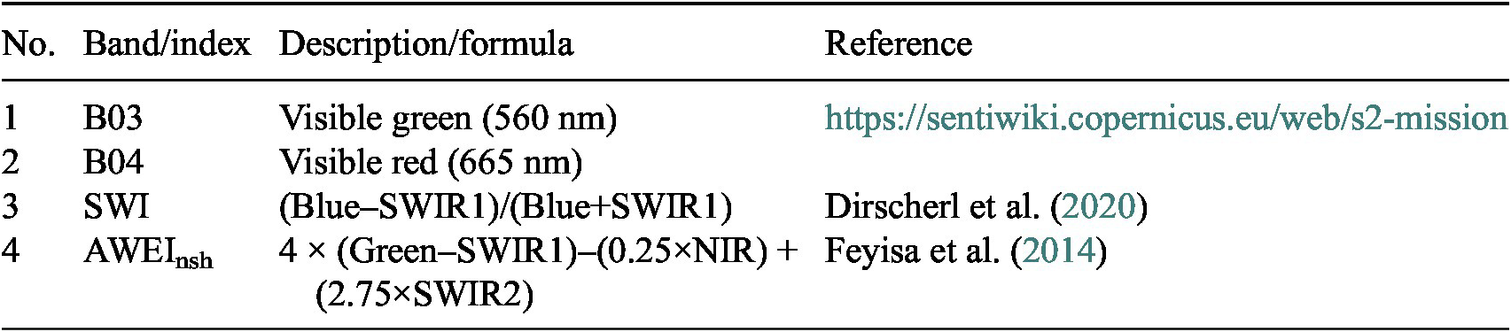





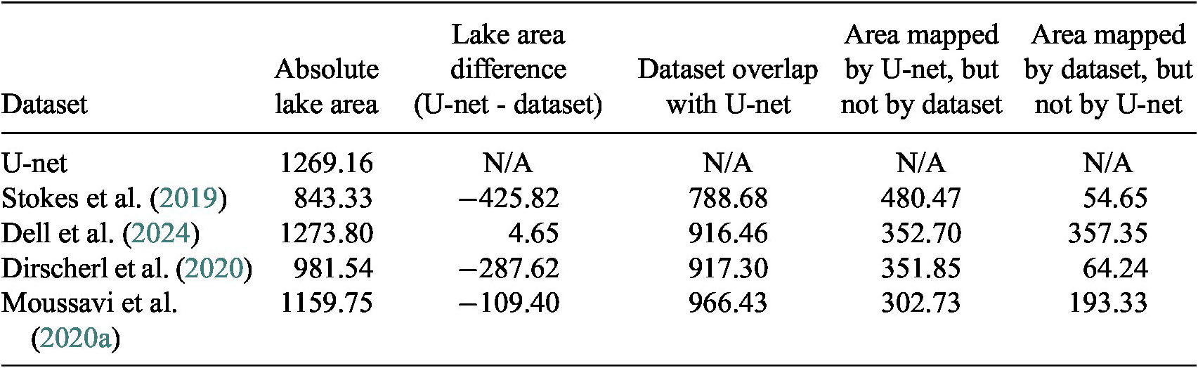

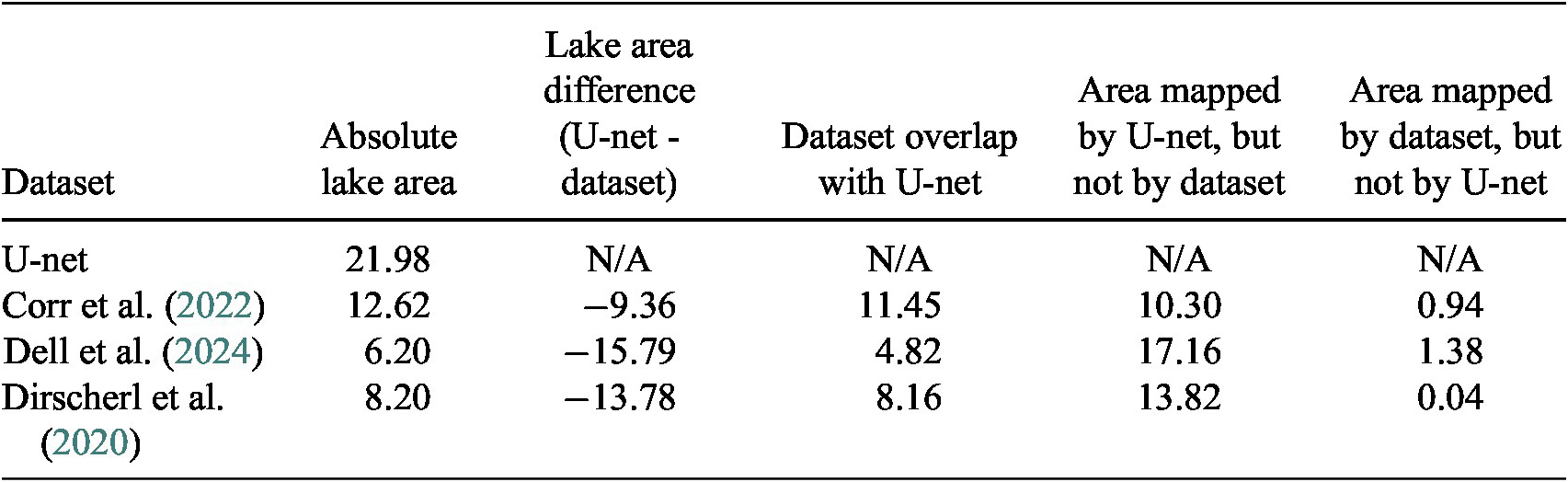


 Open access

