1. Introduction
Owing to its prevalence in natural and industrial processes, particle-laden turbulence (PLT) has attracted enduring attention in fluid dynamics and related fields. Examples include sediment transport and deposition (Bagnold Reference Bagnold2012; Salinas et al. Reference Salinas, Balachandar, Shringarpure, Fedele, Hoyal and Cantero2020, Reference Salinas, Balachandar, Shringarpure, Fedele, Hoyal, Zuniga and Cantero2021), pyroclastic flows throughout volcanic eruptions (Lube et al. Reference Lube, Breard, Esposti-Ongaro, Dufek and Brand2020), gas–solid reactors (Solé et al. Reference Solé, Martorell and Cabeza2015) and slurry pipelines (Shook & Roco Reference Shook and Roco2013), among others. Across these diverse contexts, a common challenge lies in unravelling the transport dynamics of mass, momentum and energy in PLT, where particle–turbulence interactions give rise to fascinating phenomena, with turbulence modulation being one of the most prominent. Nonetheless, the coexistence of a broad spectrum of characteristic length and time scales, combined with a vast governing parameter space, renders the modulation behaviours particularly intricate to understand (Elghobashi Reference Elghobashi1994; Eaton & Longmire Reference Eaton and Longmire2016). While considerable consensus has been reached regarding the modulation mechanisms of turbulence augmentation and attenuation in homogeneous turbulence, the situation remains less settled for wall-bounded configurations (Brandt & Coletti Reference Brandt and Coletti2022).
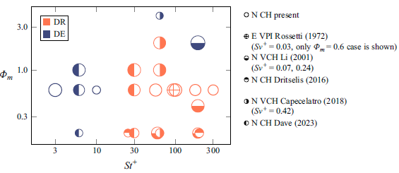
As comprehensively reviewed by Wilson (Reference Wilson1942), Soo (Reference Soo1967) and Kulick (Reference Kulick1994), the ability of inertial particles to modify the hydraulic resistance in pipes or channels has been demonstrated in experiments dating back to the early 1900s. Both drag enhancement (DE) and drag reduction (DR) have been reported, and are usually explained by the modification of turbulence intensity (e.g. Rossetti & Pfeffer Reference Rossetti and Pfeffer1972; Zisselmar & Molerus Reference Zisselmar and Molerus1979; Tsuji & Morikawa Reference Tsuji and Morikawa1982; Tsuji, Morikawa & Shiomi Reference Tsuji, Morikawa and Shiomi1984; Kulick, Fessler & Eaton Reference Kulick, Fessler and Eaton1994; Mena & Curtis Reference Mena and Curtis2020). An illuminating discussion by Hetsroni (Reference Hetsroni1989) attributed the observed turbulence attenuation or augmentation to a competition between vortex shedding and extra dissipation induced by particles. The particle Reynolds number,
 $Re_p\equiv |\boldsymbol{s}|d_p/\nu$
(with
 $\boldsymbol{s}$
denoting the fluid–particle slip velocity,
 $d_p$
the particle diameter and
 $\nu$
the kinematic viscosity), was identified as the key control parameter of such a competition. This provides a compelling rationale for the classification proposed by Gore & Crowe (Reference Gore and Crowe1989), which delineates the attenuation-augmentation boundary in centreline velocity fluctuations based on the normalised particle diameter: particles with
 $d_p/l_e\gtrsim 0.1$
augment centreline fluctuations, while particles with
 $d_p/l_e\lesssim 0.1$
attenuate them, where
 $l_e$
denotes the length scale of the energetic eddies.
However, Eaton & Longmire (Reference Eaton and Longmire2016) pointed out that the classification of Gore & Crowe (Reference Gore and Crowe1989) and Hetsroni (Reference Hetsroni1989) is, to some extent, oversimplistic, where some critical physical mechanisms were omitted and, thus, the modulation dependencies on various control parameters were not elucidated. From a dimensional analysis of the particle-laden Navier–Stokes equation, Tanaka & Eaton (Reference Tanaka and Eaton2008) mapped the turbulent kinetic energy (TKE) modification results of internal flows on a derived non-dimensional parameter, particle momentum number
 $Pa_{St}$
. This parameter incorporates flow Reynolds number (
 $Re$
) and particle Stokes number (
 $St$
), where the latter indicates the strength of particle inertia, in the form of
 $Pa_{St}=St Re_{L}^2 (\eta /L)^3$
(with
 $\eta$
denoting the Kolmogorov length scale,
 $L$
the integral scale). Their compilation of pipe and channel flow data showed that TKE attenuation occurs for
 $3\times 10^3\lt Pa_{St}\lt 10^5$
, while augmentation occurs at both lower and higher
 $Pa_{St}$
. Remarkably, the augmentation regime at low
 $Pa_{St}$
– associated with low
 $St$
and low
 $Re_p$
(Sato & Hishida Reference Sato and Hishida1996; Suzuki, Ikenoya & Kasagi Reference Suzuki, Ikenoya and Kasagi2000; Kiger & Pan Reference Kiger and Pan2002) – suggests the existence of additional turbulence production mechanisms, distinct from vortex shedding, in wall-bounded flows.
To address this inherent complexity, which arises from the coexistence and interaction of multiple mechanisms, numerical simulations offer a feasible approach. They provide detailed access to flow and particle dynamics that are difficult or even impossible to obtain experimentally, enabling deeper insights into the nature of particle–turbulence interactions (Crowe, Sharma & Stock Reference Crowe, Sharma and Stock1977; Elghobashi Reference Elghobashi1994; Balachandar & Eaton Reference Balachandar and Eaton2010; Tenneti & Subramaniam Reference Tenneti and Subramaniam2014; Kuerten Reference Kuerten2016). Recent direct numerical simulations have reported both DR (Zhao et al. Reference Zhao, Andersson and Gillissen2010, Reference Zhao, Andersson and Gillissen2013; Gao, Samtaney & Richter Reference Gao, Samtaney and Richter2023) and DE (Costa, Brandt & Picano Reference Costa, Brandt and Picano2021; Battista et al. Reference Battista, Gualtieri, Mollicone, Salvadore and Casciola2023; Gualtieri et al. Reference Gualtieri, Battista, Salvadore and Casciola2023) in internal flows without gravity. It is found that the DR is generally associated with a drastic laminarisation characterised by the near-wall flow structures, namely, the low-speed streaks become more elongated with their spanwise spacing increased (Zhao, Andersson & Gillissen Reference Zhao, Andersson and Gillissen2010; Richter & Sullivan Reference Richter and Sullivan2013, Reference Richter and Sullivan2014). In contrast, the DE is attributed to the extra shear stress and TKE production introduced by particles, as revealed by the budget analysis (Lee & Lee Reference Lee and Lee2015; Gualtieri et al. Reference Gualtieri, Battista, Salvadore and Casciola2023). These numerical studies collectively indicate a complex interplay between particle dynamics and the self-organised near-wall flow structures, see Marchioli & Soldati (Reference Marchioli and Soldati2002) and Soldati & Marchioli (Reference Soldati and Marchioli2009) for some insightful discussions.
Further studies investigating the effects of friction Stokes number
 $St^+=\tau /t_v^{{SP}}$
(with
 $\tau$
being the particle relaxation time and
 $t_v^{{SP}}$
the viscous time scale in single-phase wall-bounded turbulence) have highlighted its major role in turbulent channel flows laden with small inertial particles. Interestingly, the modulation behaviours are found to exhibit non-monotonic dependence on
 $St^+$
, as reflected in flow resistance, TKE production/dissipation as well as Reynolds stress budgets (Lee & Lee Reference Lee and Lee2015; Dritselis Reference Dritselis2016; Capecelatro, Desjardins & Fox Reference Capecelatro, Desjardins and Fox2018; Zhou et al. Reference Zhou, Zhao, Huang and Xu2020; Rupp, Mortimer & Fairweather Reference Rupp, Mortimer and Fairweather2023). Lee & Lee (Reference Lee and Lee2015) found that low-inertia particles (
 $St^+=0.5$
) enhance near-wall turbulence, while moderate-to-high inertia particles (
 $St^+=5, 35, 100$
) have an opposite impact, with the most pronounced turbulence suppression occurring at
 $St^+=35$
. Dave & Kasbaoui (Reference Dave and Kasbaoui2023) interpreted the opposite turbulence modulation and the resulting DE–DR transition as a
 $St^+$
-dependent competition between the increased particle shear stress and the reduced Reynolds shear stress, inspired by the drag modification mechanisms in turbulent polymeric flows (White & Mungal Reference White and Mungal2008; Song et al. Reference Song, Zhu, Lin, Liu and Khomami2023; Zhu et al. Reference Zhu, Wan, Lin, Liu, Lu and Khomami2023; Lin et al. Reference Lin, Song, Liu, Wan, Lu and Khomami2024). While this interpretation provides some phenomenological insights, a closed and physically grounded explanation of the observed modulation behaviours remains to be established.
While the present study focuses on the role of
 $St^+$
, it is worth noting that the PLT is also influenced by other factors, including gravitational settling, mass loading (
 $\Phi _m$
) and flow Reynolds number (
 $Re$
). It is well acknowledged that gravity makes heavy particles become disengaged from turbulent flows, known as the crossing-trajectory effect (Maxey Reference Maxey1987; Marchioli, Picciotto & Soldati Reference Marchioli, Picciotto and Soldati2007). As revealed by Xu, Xu & Xi (Reference Xu, Xu and Xi2024), in wall-sheared thermal turbulence, gravitational effects influence particle motion across a wide range of Stokes numbers. At medium Stokes numbers, complex interactions between gravity and turbulence lead to pronounced spatial inhomogeneity and preferential concentration, while at large Stokes numbers, gravity dominates, resulting in linear settling behaviour and rendering the particles nearly unresponsive to the carrier flow. Bragg, Richter & Wang (Reference Bragg, Richter and Wang2021a
,Reference Bragg, Richter and Wang
b
) demonstrated that the near-wall particle concentration is highly dependent on the settling number,
 $Sv^+\equiv g\tau /u_\tau$
, where
 $g$
is the gravitational acceleration and
 $u_\tau$
the friction velocity (Bec, Gustavsson & Mehlig Reference Bec, Gustavsson and Mehlig2024). Considering the two-way coupling, the interplay between gravity-driven particle dynamics and flow structures makes the turbulence modulation even more complicated. While wall-normal gravity breaks the intrinsic symmetry of channel flows (Lee & Lee Reference Lee and Lee2019), streamwise-aligned gravity introduces a continuous energy input through the conversion of gravitational potential energy (Capecelatro, Desjardins & Fox Reference Capecelatro, Desjardins and Fox2015; Frankel et al. Reference Frankel, Pouransari, Coletti and Mani2016). With gravity included, Capecelatro et al. (Reference Capecelatro, Desjardins and Fox2018) found a non-monotonic dependence of turbulence modulation on particle mass loading
 $\Phi _m$
. A transition in turbulence generation mechanisms is revealed from mean-shear production to a so-called drag production stemming from mean interphase slip velocities. Such a non-monotonic effect of mass loading on turbulence modulation was also reported for zero-gravity channel flows (Zhou et al. Reference Zhou, Zhao, Huang and Xu2020). In addition, some studies have investigated the role of the
 $Re$
in affecting the scaling properties of particle-laden turbulence (e.g. Bernardini Reference Bernardini2014; Richter Reference Richter2015; Jie et al. Reference Jie, Cui, Xu and Zhao2022).
In the present study, we investigate the turbulence modulation in zero-gravity, fully developed incompressible channel turbulence at
 $Re_b\equiv U_b h/\nu =5150$
(with
 $U_b$
denoting the bulk flow velocity and
 $h$
the channel half-height), laden with a dilute suspension of small heavy particles (particle diameter
 $d_p^+\approx 0.5$
, density ratio
 $\rho _p/\rho \gg 1$
and volume fraction
 $\phi _v\ll 1$
). Under such conditions, extra turbulence production due to vortex shedding is negligible. Furthermore, guided by Tanaka & Eaton (Reference Tanaka and Eaton2008), Lee & Lee (Reference Lee and Lee2015) and Dave & Kasbaoui (Reference Dave and Kasbaoui2023), we focus on the effects of particle inertia, characterised by
 $St^+$
, while keeping the mass loading fixed at
 $\Phi _m\equiv \phi _v\rho _p/\rho =0.6$
. A full transition pathway – from DE to DR before recovering the single-phase state – is observed through a series of four-way coupled point-particle direct numerical simulation (PP-DNS) with
 $St^+$
increasing from
 $3$
to
 $300$
. A systematic statistical description of the transport processes in PLT (Subramaniam Reference Subramaniam2020; Subramaniam & Balachandar Reference Subramaniam and Balachandar2022) is employed to elucidate the particle–turbulence interactions. We uncover an interesting mechanism, termed particle-induced extra transport, which originates from the mean gradient in wall-bounded flows and competes against the extra dissipation in multiple aspects – mean momentum transport, TKE production and dissipation, as well as the self-sustaining process of Reynolds stresses. Following the ideas of Saffman (Reference Saffman1962), the limit behaviours of extra transport and extra dissipation at
 $St^+\to 0$
or
 $\infty$
are studied analytically to explain the observed
 $St^+$
dependencies. This yields a comprehensive physical picture of the two competing mechanisms in a statistical sense, offering insights into the intricate behaviours of turbulence modulation in wall-bounded flows.
2. The deterministic description
Since we are considering a dilute suspension of small heavy particles (
 $\phi _v\ll 1$
,
 $\rho _p/\rho \gg 1$
and
 $d_p\lt \eta$
), the continuous fluid motion is governed by the incompressible Navier–Stokes equations
 \begin{align} \frac {\partial u_i}{\partial x_i} &= \,0,\\[-10pt]\nonumber \end{align}
 \begin{align} \frac {\partial u_{i}}{\partial t}+u_{j}\frac {\partial u_{i}}{\partial x_j} & = -\frac {1}{\rho }\frac {\partial p}{\partial x_i}+\nu \frac {\partial ^2 u_i}{\partial x_j\partial x_j}+{\mathcal{F}_i}, \end{align}
where
 ${\boldsymbol{u}}=(u_i), \,i=1,2,3$
denotes the fluid velocity;
 $p$
represents the pressure;
 $\rho$
the density and
 $\nu =\mu /\rho$
the kinematic viscosity with
 $\mu$
being the dynamic viscosity of the fluid phase. The particle feedback force
 $\mathcal{F}_i$
appearing in the right-hand side of (2.2) can be formally written as a summation over all
 $N_p$
particles (Crowe et al. Reference Crowe, Schwarzkopf, Sommerfeld and Tsuji2011),
 \begin{equation} \mathcal{F}_i= -\frac {1}{\rho }\sum _{n=1}^{N_p}\delta \big(\boldsymbol{x}-\boldsymbol{x}_p^{(n)}\big)F_i^{(n)}. \end{equation}
Here, the particle indexed by superscript
 $(n)$
has the velocity
 $\boldsymbol{v}=(v_i),\,i=1,2,3$
, and the force acting on it through interphase momentum coupling is denoted by
 $F_i$
. The Dirac delta function
 $\delta (\,\cdot \,)$
, which is approximated numerically by a non-singular mollification kernel (Capecelatro & Desjardins Reference Capecelatro and Desjardins2013), maps the feedback located at point-particle position
 $\boldsymbol{x}_p(t)$
to the Eulerian field.
The dispersed particle phase is described in a Lagrangian perspective. Considering the monodispersed situation where all physical properties of particles (e.g. the density
 $\rho _p$
, the diameter
 $d_p$
, the mass
 $m_p=\rho _p\pi d_p^3/6$
) are identical, the temporal evolution of each point particle is governed by (Crowe et al. Reference Crowe, Schwarzkopf, Sommerfeld and Tsuji2011)
 \begin{align} \frac {\textrm{d}\boldsymbol{x}_{p}^{(n)}}{\textrm{d}t} = \boldsymbol{v}^{(n)},\end{align}
 \begin{align} m_p\frac {\textrm{d}\boldsymbol{v}^{(n)}}{\textrm{d}t} = \boldsymbol{F}^{(n)}=3\pi \mu d_p\left[{\boldsymbol{u}}\left(\boldsymbol{x}_p^{(n)},t\right)-\boldsymbol{v}^{(n)}\right]f_D\left(Re_p^{(n)}\right). \end{align}
Note that for small heavy particles of interest, interphase momentum couplings, except the Stokes drag, are negligible (Bec et al. Reference Bec, Gustavsson and Mehlig2024). Gravity is ignored in the present work to focus on the effects of particle inertia, implying a zero particle settling number,
 $Sv^+\equiv {\tau g}/{u_\tau }$
(Brandt & Coletti Reference Brandt and Coletti2022; Bec et al. Reference Bec, Gustavsson and Mehlig2024). The finite Reynolds number effect can be taken into account by introducing the widely adopted Schiller–Naumann correlation
 $f_D=1+0.15 Re_p^{0.687}$
(Schiller Reference Schiller1933), with particle Reynolds number defined as
 $Re_p\equiv {\rho |{\boldsymbol{u}}-\boldsymbol{v}|d_p}/{\mu }$
. By introducing the particle relaxation time
 $\tau \equiv \rho _pd_p^2/(18\mu )$
and the slip velocity
 $\boldsymbol{s}={\boldsymbol{u}}-\boldsymbol{v}=(s_i),\,i=1,2,3$
, (2.5) can be rewritten as
 \begin{align} \frac { {\textrm{d}v_i^{(n)}} }{ {\textrm{d}t} } = \frac {F_i^{(n)}}{m_p} = \frac {f_D s_i^{(n)}}{\tau }. \end{align}
Strictly speaking,
 $\boldsymbol{u}(\boldsymbol{x}_p^{(n)},t)$
in (2.5) represents the instantaneous flow velocity at
 $\boldsymbol{x}_p^{(n)}$
undisturbed by the presence of particle
 $n$
(Maxey & Riley Reference Maxey and Riley1983). In two-/four-way coupled Euler–Lagrange simulations, approximating it by the disturbed flow velocity introduces a self-induced velocity error, which is proportional to the particle diameter to grid spacing ratio
 $d_p/\varDelta$
(Boivin, Simonin & Squires Reference Boivin, Simonin and Squires1998). Numerous correction approaches have been developed in previous studies to refine the computational accuracy of PP-DNS (Gualtieri et al. Reference Gualtieri, Picano, Sardina and Casciola2015; Horwitz & Mani Reference Horwitz and Mani2016; Ireland & Desjardins Reference Ireland and Desjardins2017; Esmaily & Horwitz Reference Esmaily and Horwitz2018; Balachandar, Liu & Lakhote Reference Balachandar, Liu and Lakhote2019; Fukada, Takeuchi & Kajishima Reference Fukada, Takeuchi and Kajishima2019; Poustis et al. Reference Poustis, Senoner, Zuzio and Villedieu2019; Evrard, Denner & van Wachem Reference Evrard, Denner and van Wachem2020). It is now widely accepted that self-induced velocity corrections are unnecessary for particles smaller than approximately
 $0.1 d_p/\varDelta$
(Horwitz & Mani Reference Horwitz and Mani2018; Balachandar et al. Reference Balachandar, Liu and Lakhote2019). Accordingly, in the present work, the particle size is designed to be small enough and a low-order scheme (trilinear interpolation) is employed to calculate
 $\boldsymbol{u}(\boldsymbol{x}_p^{(n)},t)$
, which helps mitigate the self-induced velocity error (Horwitz & Mani Reference Horwitz and Mani2020; Horwitz Reference Horwitz2023).
The inter-particle collisions can be described using the hard-sphere model (HSM, Hoomans et al. Reference Hoomans, Kuipers, Briels and van Swaaij1996; Sundaram & Collins Reference Sundaram and Collins1997; Mallouppas & van Wachem Reference Mallouppas and van Wachem2013), which is well suited to dilute suspensions of rigid spheres considered here. Specifically, instead of resolving the interactions during particle–particle contacting, HSM directly computes the results of binary collisions through
 \begin{align} \boldsymbol{v}^{(n)} = & \, \boldsymbol{v}^{(n)}_0-\frac {1+e}{2}\left[{\boldsymbol \xi }\cdot \left(\boldsymbol{v}^{(n)}_0-\boldsymbol{v}^{(m)}_0\right)\right]{\boldsymbol \xi },\\[-10pt]\nonumber \end{align}
 \begin{align} \boldsymbol{v}^{(m)} = & \, \boldsymbol{v}^{(m)}_0+\frac {1+e}{2}\left[{\boldsymbol \xi }\cdot \left(\boldsymbol{v}^{(n)}_0-\boldsymbol{v}^{(m)}_0\right)\right]{\boldsymbol \xi }, \end{align}
where
 $\boldsymbol{v}^{(n)}$
and
 $\boldsymbol{v}^{(m)}$
denote the post-collision velocities, and
 $\boldsymbol{v}^{(n)}_0$
and
 $\boldsymbol{v}^{(m)}_0$
the pre-collision velocities;
 $\boldsymbol{\xi }$
is the unit vector pointing from the centre of particle
 $n$
to the centre of particle
 $m$
; and
 $e$
denotes the coefficient of restitution. In the present simulations, both particle–particle and particle–wall collisions are assumed to be elastic (
 $e=1$
) to exclude the collisional dissipation. Practically, dry collisions between hard spherical particles exhibit a coefficient of restitution close to unity (taking steel and glass particles as examples,
 $e\in (0.95,1)$
, see Yang & Hunt Reference Yang and Hunt2006), and thus the assumption of elastic collision applies very well.
Based on the above mentioned equations, we obtain a closed, deterministic description of particle-laden flows. Integrating the Lagrangian particle tracking (2.4)–(2.5), particle back-reaction (2.3) and inter-particle collision (2.7)–(2.8), this description serves as the basis of four-way coupled PP-DNS. An early classification proposed by Elghobashi (Reference Elghobashi1991, Reference Elghobashi1994) conjectured that the inter-particle collision plays a role only when the mean volume fraction
 $\phi _v$
is above
 $10^{-3}$
. However, preferential concentration and turbophoresis can result in a significant increase in local volume fraction, where the inter-particle collision comes into play, and thus the four-way coupling becomes indispensable even at
 $\phi _v\lt 10^{-3}$
(Subramaniam & Balachandar Reference Subramaniam and Balachandar2022). Numerous experimental and numerical studies have well documented the critical role of inter-particle collisions in particle transport and flow modulation (Li et al. Reference Li, McLaughlin, Kontomaris and Portela2001; Kussin & Sommerfeld Reference Kussin and Sommerfeld2002; Caraman, Borée & Simonin Reference Caraman, Borée and Simonin2003; Kuerten & Vreman Reference Kuerten and Vreman2015; Esmaily et al. Reference Esmaily, Villafane, Banko, Iaccarino, Eaton and Mani2020).
3. The statistical description
For turbulent flows laden with a large number of small heavy particles, it has been established that the statistical description is advantageous for theoretical analysis of the collective behaviours of the particle ensemble (Elghobashi Reference Elghobashi1994; Subramaniam Reference Subramaniam2020; Subramaniam & Balachandar Reference Subramaniam and Balachandar2022). The point-based statistical description of particle-laden turbulent flows integrates turbulence theory for the fluid phase with kinetic theory for the particle phase (Jenkins & Savage Reference Jenkins and Savage1983; Reeks Reference Reeks1991, Reference Reeks1992). This theoretical framework has been used to identify the mechanisms governing mean particle drifting (Reeks Reference Reeks1983; Guha Reference Guha1997; Johnson, Bassenne & Moin Reference Johnson, Bassenne and Moin2020), model the particle transport in random media and turbulent flows (Swailes & Darbyshire Reference Swailes and Darbyshire1997; Swailes, Sergeev & Parker Reference Swailes, Sergeev and Parker1998; Bragg, Swailes & Skartlien Reference Bragg, Swailes and Skartlien2012), and construct macroscale Euler–Euler models (where the particle phase is described by the moment equations) for fluid–particle systems (Fox Reference Fox2007, Reference Fox2012, Reference Fox2014; Fox et al. Reference Fox, Posey, Houim and Laurent2024). Notably, while previous studies (Caraman et al. Reference Caraman, Borée and Simonin2003; Vreman Reference Vreman2007; Richter & Sullivan Reference Richter and Sullivan2013; Capecelatro et al. Reference Capecelatro, Desjardins and Fox2015, Reference Capecelatro, Desjardins and Fox2018) have employed some of the moment equations to analyse turbulence modulation, the fundamental role of particle inertia – as quantified by the Stokes number – remains a rather open issue. This knowledge gap forms the central focus motivating the present study. Through the coupling of the two-phase moment equations, we demonstrate how this approach yields new insights into particle–turbulence interactions, particularly in wall-bounded geometries. To this purpose, key definitions in the point-based statistical description and detailed derivations of moment equations are provided here and in Appendix A.
Since all particles are considered identical, their statistical behaviours are characterised by the one-particle probability distribution
 $f$
in the six-dimensional phase space
 $(\boldsymbol{x},\boldsymbol{v})$
with the normalisation condition
 $\int f\,\textrm{d}\boldsymbol{x} \textrm{d}\boldsymbol{v}=1$
(see Appendix A.1 for a formal definition). Without any assumption and modelling of phase-space transports, the evolution of
 $f(\boldsymbol{x},\boldsymbol{v};t)$
is governed by the following equation (Lifschitz & Pitajewski Reference Lifschitz and Pitajewski1981):
 \begin{equation} \frac {\partial f}{\partial t}+\frac {\partial (v_k f)}{\partial x_k}+\frac {1}{m_p}\frac {\partial (F_k f)}{\partial v_k}=\left (\frac {\partial f}{\partial t}\right )_{{coll}}. \end{equation}
The right-hand-side term
 $(\partial f/\partial t)_{{coll}}$
, known as the collision integral, represents the contribution of inter-particle collisions on the phase-space evolution. Here, the force acting on particles,
 $F_k$
, depends on velocity through the Stokes drag and is thus dissipative. In this work, (3.1) will not be handled directly. Instead, we deal with the derived physical-space transport equations, which are also referred to as the moment equations.
It is well known that, after the particles are released into a fully developed turbulent channel flow, the two-phase system will gradually approach a statistically stationary state. Furthermore, the intrinsic property of single-phase channel turbulence, namely, statistical homogeneity in the streamwise and the spanwise directions, is preserved, as verified by numerous studies (Marchioli et al. Reference Marchioli, Soldati, Kuerten, Arcen, Tanière, Goldensoph, Squires, Cargnelutti and Portela2008; Soldati & Marchioli Reference Soldati and Marchioli2009). Hence, the mean particle concentration can be formally defined as (Elghobashi Reference Elghobashi1994; Johnson et al. Reference Johnson, Bassenne and Moin2020)
 \begin{align} c(y,t) \equiv & \idotsint f(\boldsymbol{x},\boldsymbol{v};t)\,\textrm{d} \boldsymbol{v} \textrm{d}x \textrm{d}z. \end{align}
This is also referred to as the wall-normal probability density, which inherits the normalisation condition from
 $f$
. To effectively characterise the near-wall accumulation of particles, it is common to consider the normalised particle concentration
 $\hat {c}\equiv c/c_b$
, where the bulk concentration is
 $c_b = \int _0^{L_y} c \textrm { d} y / L_y = 1/L_y$
and
 $L_y$
denotes the domain size in
 $y$
direction. The particle mass loading profile is then formulated as
 \begin{equation} C(y,t) =\Phi _m \hat {c} = \Phi _m L_y \idotsint f(\boldsymbol{x},\boldsymbol{v};t)\,\textrm{d} \boldsymbol{v} \textrm{d}x \textrm{d}z. \end{equation}
Moreover, the one-dimensional particle average of a given function
 $A(\boldsymbol{x},\boldsymbol{v})$
is defined as
 \begin{equation} \langle A\rangle (y,t) \equiv \frac {1}{c(y,t)} \idotsint A f\,\textrm{d}\boldsymbol{v} \textrm{d}x \textrm{d}z. \end{equation}
Clearly, setting
 $A=1$
in (3.4) recovers (3.2). The above mentioned definitions reflect the assumed statistical homogeneity in streamwise and spanwise directions. It should be noted that the particle average
 $\langle \,\cdot \,\rangle$
can act not only on particle variables, but also on flow variables. For example,
 $\langle u_1\rangle$
means the averaged streamwise flow velocity sampled at particle positions; therefore, in conception, different from its Reynolds averaged counterpart
 $\bar {u}_1$
due to the preferential sampling nature of inertial particles (Bragg et al. Reference Bragg, Swailes and Skartlien2012; Capecelatro, Desjardins & Fox Reference Capecelatro, Desjardins and Fox2016). Unlike the Reynolds decomposition (
 $A=\overline {A}+A'$
), the fluctuating part of variable
 $A$
with regards to its particle average is denoted by
 $A^\circ \equiv A-\langle A\rangle$
hereafter.
Following a procedure analogous to that of deriving the Navier–Stokes equations from the Boltzmann equation (Kremer Reference Kremer2010), the averaged transport equations for the particle phase can be easily obtained. Once the two-phase system approaches the statistically stationary state, where
 ${\partial \langle \,\cdot \,\rangle }/{\partial t}={\partial \overline {\vphantom {(}\cdot \vphantom {)}}}/{\partial t}=0$
and
 $C(y,t)=C(y)$
, the particle-phase continuity equation leads to
 $\langle v_i\rangle =(\langle v_1\rangle (y),\,0,\,0)$
; and the corresponding momentum equation is formulated as
 \begin{equation} \frac {\textrm{d} (C\langle v_iv_2\rangle )}{\textrm{d} y} - {C\langle \widehat {F_i}\rangle } = 0. \end{equation}
Here, we define
 $\widehat {F}_i\equiv F_i/m_p$
and (3.5) represents the conservation of particle-phase momentum per unit mass, namely, a balance realised between particle transport (the first term) and fluid driving force (the second term). Hereafter, both particle average and Reynolds average are practically approximated by a combined horizontal and temporal average. The non-uniform
 $C(y)$
characterises the compressible nature of the particle phase (Fox Reference Fox2014), which is reflected in the near-wall accumulation due to a combined effect of segregation, turbophoretic drift, diffusional drift, among other mechanisms (Caporaloni et al. Reference Caporaloni, Tampieri, Trombetti and Vittori1975; Reeks Reference Reeks1983; Brooke, Hanratty & McLaughlin Reference Brooke, Hanratty and McLaughlin1994; Guha Reference Guha1997, Reference Guha2008; Marchioli & Soldati Reference Marchioli and Soldati2002; Soldati & Marchioli Reference Soldati and Marchioli2009). Furthermore, (3.5) can be inherently connected with the Reynolds averaged momentum equation of the fluid phase through (Appendix A.4)
 \begin{equation} \overline {\mathcal{F}}_i=-C\langle \widehat {F_i} \rangle . \end{equation}
Such a procedure can also be applied to the second-order particle velocity moments, similar to that of deriving the TKE (
 $k=\overline {u'_iu'_i}/2$
) and Reynolds stress (
 $r_{ij}=\overline {u'_iu'_j}$
) budgets, leading to the budget equations of particle-phase fluctuating kinetic energy (PFKE),
 $k_p \equiv \langle v_i^\circ v_i^\circ \rangle /2$
, and particle-phase Reynolds stresses,
 $r_{p,ij}\equiv \langle v_i^\circ v_j^\circ \rangle$
. The derivations of these transport equations and the coupling relations between the fluid and particle phases are elaborated in Appendices A.2–A.4.
4. Dataset descriptions
In the present study, near-incompressible particle-laden channel flows are solved using the GPU-accelerated four-way coupled PP-DNS code we developed recently for the compressible PLT problems (Liao et al. Reference Liao, Chen, Wan, Liu and Lu2024) based on STREAmS (Bernardini et al. Reference Bernardini, Modesti, Salvadore and Pirozzoli2021). To minimise the compressibility effects, a low Mach number of
 $0.2$
is considered according to Gerolymos & Vallet (Reference Gerolymos and Vallet2014), Modesti & Pirozzoli (Reference Modesti and Pirozzoli2016) and Ruan & Xiao (Reference Ruan and Xiao2024). The numerical solver has been extensively validated by accurately reproducing the statistical results of several benchmark simulations of incompressible particle-laden channel flows (Marchioli et al. Reference Marchioli, Soldati, Kuerten, Arcen, Tanière, Goldensoph, Squires, Cargnelutti and Portela2008; Kuerten, Van Der Geld & Geurts Reference Kuerten, Van Der Geld and Geurts2011; Johnson et al. Reference Johnson, Bassenne and Moin2020; Dave & Kasbaoui Reference Dave and Kasbaoui2023), encompassing all three interphase coupling levels (namely, the one-, two- and four-way couplings), see Liao et al. (Reference Liao, Chen, Wan, Liu and Lu2024) and Appendix C.1 for code validation.
Here, we briefly introduce the numerical methods adopted in this GPU-based solver of high parallel efficiency. The governing equations of the fluid phase are solved on a rectilinear grid using a high-order finite-difference method. Specifically, the convective and viscous terms are discretised using an eighth-order energy-preserving scheme (Pirozzoli Reference Pirozzoli2010) and a sixth-order central scheme, respectively. A three-stage, third-order Runge–Kutta (RK) scheme is used for time integration (Spalart, Moser & Rogers Reference Spalart, Moser and Rogers1991; Bernardini et al. Reference Bernardini, Modesti, Salvadore and Pirozzoli2021). The flow variables seen by particles are computed by trilinear interpolation. Then the particle feedback is distributed onto the surrounding 8 grid points using the same weight coefficients as interpolation (Eaton Reference Eaton2009), forming a numerical approximation of (2.3). The collision detection is achieved using the spatial subdivision technique. The third-order total variation diminishing RK is applied to advance particle variables in time (Gottlieb & Shu Reference Gottlieb and Shu1998). Further details on the numerical techniques and GPU implementation strategies can be found from Liao et al. (Reference Liao, Chen, Wan, Liu and Lu2024).
Schematic of the computational domain used in the present simulations. The contour plot represents an instantaneous streamwise velocity field for the St030 case. Half of the computational domain is set to be translucent to visualise the dispersed particles (light blue spheres).

For all the simulations conducted, the bulk Reynolds number
 $Re_b\equiv U_b h/\nu =5150$
is fixed (a uniform streamwise forcing term is added, dynamically evaluated at each time step to directly enforce a constant flow rate in time, as in Huang, Coleman & Bradshaw Reference Huang, Coleman and Bradshaw1995; Modesti & Pirozzoli Reference Modesti and Pirozzoli2016) and, correspondingly, the friction Reynolds number
 $Re_\tau \equiv u_\tau h/\nu$
is obtained around
 $300$
. Here,
 $U_b$
denotes the bulk velocity and
 $h$
the channel half-height. The wall units are defined as follows: the friction velocity
 $u_\tau \equiv \sqrt {\tau _w/\rho }$
(hereafter, subscript
 $w$
is used to denote quantities at the wall), the viscous length scale
 $\delta _v\equiv \nu /u_\tau$
and the viscous time scale
 $t_v\equiv \nu /u_\tau ^2$
. The computational box size is
 $L_x\times L_y\times L_z=4\pi h\times 2h\times 2\pi h$
, as illustrated in figure 1. The grid sizes used in the
 $x,y,z$
directions are
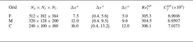
 $N_x\times N_y\times N_z=512\times 192\times 384$
, corresponding to grid spacings of
 $\Delta x^+\approx 7.5$
,
 $0.4\lesssim \Delta y^+\lesssim 5.6$
,
 $\Delta z^+\approx 5.0$
. As a common treatment, a hyperbolic tangent stretching is applied in the wall-normal direction to cluster grid nodes close to the wall, obtaining a minimum spacing of
 $\Delta y_{{min}}^+\approx 0.4$
(Modesti & Pirozzoli Reference Modesti and Pirozzoli2016; Bernardini et al. Reference Bernardini, Modesti, Salvadore and Pirozzoli2021). The grid convergence is examined for both particle-free and particle-laden cases, which is detailed in Appendix C.2. Hereafter, variables with superscript ‘
 $+$
’ are non-dimensionalised by the wall units.
Simulation set-ups for the particle phase. The particle volume fraction
 $\phi _v$
varies from
 ${\sim} 10^{-3}$
to
 ${\sim} 10^{-5}$
corresponding to a mass loading
 ${\Phi }_m$
fixed at 0.6, lying in the (semi-)dilute suspension regime.
 $N_s$
and
 $\mathcal{T}$
denote the number of snapshots and the time window widths, respectively, adopted in each case for calculating the statistics.

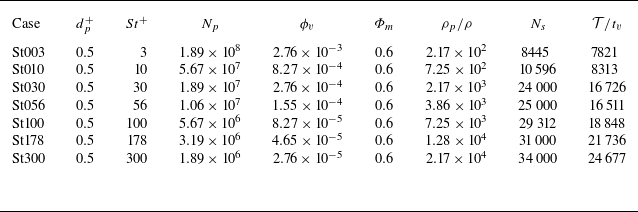
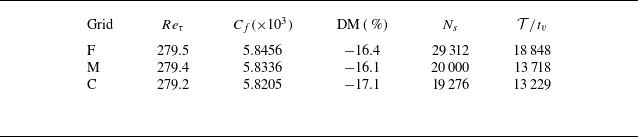
Initially, particles are randomly released into a fully developed single-phase channel flow, with velocities interpolated by the surrounding fluid. The streamwise and spanwise boundary conditions for particles are assumed periodic to maintain a constant mass loading. The parameter set-ups for the particle phase are listed in table 1, having a wide Stokes number range of two orders, i.e.
 $3\leqslant St^+\leqslant 300$
. The particle diameter is fixed at
 $d_p^+=d_p/\delta _v^{{SP}}=0.5$
and thus the friction Stokes number
 $St^+\equiv \tau /t_v^{{SP}}=(\rho _p/\rho )(d_p/\delta _v^{{SP}})^2/18$
is determined by density ratio
 $\rho _p/\rho$
. Hereafter, the abbreviation
 $\text{SP}$
denotes the variables or the situation for the single-phase flow. The maximum density ratio in the present set-ups is
 $2.17\times 10^4$
, which can be readily attained in certain low-density gaseous environments. For example, for sand or dust particles with
 $\rho _p \approx 2600\,{\textrm{kg}}\,m^{-3}$
suspended in the high-altitude regions of Earth – or in the Martian atmosphere, whose density is only
 $\approx 1\,\%$
of the standard sea-level atmospheric density on Earth – the solid–gas density ratio easily reaches
 $O(10^4)\sim O(10^5)$
. The particle mass loading
 ${\Phi }_m$
is fixed at
 $0.6$
for all cases, which is large enough to obtain a considerable turbulence modulation (Kulick Reference Kulick1994; Li et al. Reference Li, McLaughlin, Kontomaris and Portela2001; Zhou et al. Reference Zhou, Zhao, Huang and Xu2020; Dave & Kasbaoui Reference Dave and Kasbaoui2023). The effects of mass loading are briefly discussed in Appendix B.2. After the flow system reaches a statistically stationary state, ensemble averaging is performed on
 $N_s=8445{-} 34\,000$
snapshots to yield flow and particle statistics, corresponding to a sampling window size of
 $\mathcal{T}^+=\mathcal{T}/t_v\sim O(10^4)$
(see the last two columns in table 1). The time series of wall shear stress
 $\tau _w$
during the sampling window are depicted in figure 2 to indicate the statistical convergence achieved. Additionally, the particle concentration and other variables are sampled and averaged on a wall-normal stretched grid, using the same discretisation as the fluid-phase solver, i.e. the slabs adopted for computing particle-phase statistics are centred around each grid point.
Time series of wall shear stress
 $\tau _w(t)$
during the sampling window (solid lines). The dashed lines of the corresponding colours represent the time-averaged quantities.

5. Results and discussions
5.1. The mean flow properties
At first, we briefly examine the mean flow properties to establish a basic impression of the particle inertial effects on turbulence modulation. Figure 3
 $(a)$
depicts the mean flow velocity profiles for all cases. Compared with the single-phase result indicated by a solid grey curve, the linear scaling in the viscous sublayer remains, while the velocity profile around the logarithmic layer is significantly altered. In the logarithmic layer, the mean velocity is shifted downwards due to the introduction of particles at
 $St^+=3$
. As the Stokes number increases to
 $56{-} 100$
, the mean velocity increases successively, exceeding the single-phase one. With a further increase of
 $St^+$
to
 $300$
, the mean velocity decreases and tends to approach the single-phase profile. This variation of the mean flow velocity profile with regards to the Stokes number corresponds to a non-monotonic modification of wall shear stress, i.e. an intriguing flow transition from a drag-enhanced to a drag-reduced regime and subsequently approaching the single-phase state, as substantiated in the next section.
Mean profiles of:
 $(a)$
streamwise flow velocity in wall units;
 $(b)$
streamwise particle velocity in outer units;
 $(c)$
streamwise particle velocity in wall units and
 $(d)$
normalised particle concentration.

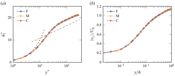
Given its critical role in momentum and energy transport, the mean particle velocity,
 $\langle v_1\rangle$
, is also examined for different Stokes numbers in figure 3
 $(b,c)$
. It is demonstrated that, as
 $St^+$
increases, the mean particle velocity profile flattens progressively, especially in the near-wall region. This trend has been explained by Johnson (Reference Johnson2020) and Liao et al. (Reference Liao, Chen, Wan, Liu and Lu2024) as follows: with the increase of
 $St^+$
, the particle inertia tends to dominate over the Stokes drag exerted by the background flow, leading to an increasingly stronger tendency for the particle phase to approach a so-called many-particle system that has an homogeneous and isotropic equilibrium state. Moreover, the particle concentration close to the wall exhibits a substantial decrease versus
 $St^+$
, see figure 3
 $(d)$
. It deviates from the pattern observed in one-way coupled simulations, where turbophoresis is found leading to a dramatic increase of near-wall particle concentration over
 $2{-} 3$
orders of magnitude compared with the uniform distribution and the highest accumulation typically occurring at
 $St^+\approx 30$
(Marchioli & Soldati Reference Marchioli and Soldati2002; Jie et al. Reference Jie, Cui, Xu and Zhao2022). This deviation can be attributed to the synergistic effect of particle back-reaction and inter-particle collision. The former alters the intrinsic length and time scales of near-wall coherent structures, which are crucial for the preferential accumulation of inertial particles (Motoori, Wong & Goto Reference Motoori, Wong and Goto2022; Jie et al. Reference Jie, Cui, Xu and Zhao2022). The latter induces a strong diffusion of the particle phase, preventing excessive clustering and promoting a more uniform distribution.
5.2. The drag properties
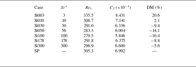
We then focus on the drag properties, which are widely regarded as crucial in wall-bounded turbulence of practical relevance. The overall statistical results are summarised in table 2. It is intriguing to find that the drag modification depends non-monotonically on the Stokes number and the system experiences both drag-enhancement (DE,
 $St^+\leqslant 10$
) and drag-reduction (DR,
 $St^+\geqslant 30$
) regimes. Specifically, the maximum DE occurs at the lowest
 $St^+$
, with a smooth transition from DE to DR as
 $St^+$
increases, where
 $St^+ \approx 10$
marks the critical point. Further increasing the Stokes number, the flow statistics indicate a tendency to return to the single-phase state, resulting in a maximum DR at
 $St^+\approx 100$
.
Overall statistics of the present simulations. Here, the skin-friction coefficient is
 $C_f\equiv 2\tau _w/(\rho U_b^2)$
. The drag-modification coefficient is defined as
 $\text{DM}\equiv (C_f-C_f^{{SP}})/C_f^{{SP}}$
.

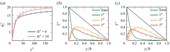
Such a DE–DR–SP transition can be substantiated by the shear stress balance (SSB, Costa et al. Reference Costa, Brandt and Picano2021; Dave & Kasbaoui Reference Dave and Kasbaoui2023)
 \begin{equation} \underbrace {\vphantom {\int _{0}^{y}}\mu \frac {\textrm{d} \bar {u}_{1}}{\textrm{d}y}}_{\bar {\tau }^{\textit{V}}} \underbrace {\vphantom {\int _{0}^{y}}-\rho \overline {u'_1u'_2}}_{\bar {\tau }^{\textit{T}}} +\underbrace {\vphantom {\int _{0}^{y}}\rho \int _{0}^{y}\overline {\mathcal{F}}_1\,\textrm{d}y}_{\bar {\tau }^{\textit{P}}} =\tau _w\left (1-\frac {y}{h}\right ). \end{equation}
Here,
 $\bar {\tau }^{\textit{V}}$
denotes the viscous shear stress of mean flow,
 $\bar {\tau }^{\textit{T}}$
the Reynolds shear stress of turbulent motions and
 $\bar {\tau }^{\textit{P}}$
the extra shear stress induced by particles. Essentially, these shear stresses reflect the transport of fluid-phase streamwise momentum in the wall-normal direction. Following Gualtieri et al. (Reference Gualtieri, Battista, Salvadore and Casciola2023), their contributions to the skin-friction coefficient can be quantified by the well-known FIK-type integrals (Fukagata, Iwamoto & Kasagi Reference Fukagata, Iwamoto and Kasagi2002), i.e. integrating (5.1) twice and reading as
 \begin{equation} \underbrace {\vphantom {\frac {6}{h^2U_b^2}}\frac {6}{Re_b}}_{C_f^{\textit{V}}} +\underbrace {\vphantom {\frac {6}{h^2U_b^2}}\frac {6}{h^2U_b^2}\int _{0}^{h}(h-y)\big(-\overline {u'_1u'_2}\big)\,\textrm{d}y}_{C_f^{\textit{T}}} +\underbrace {\vphantom {\frac {6}{h^2U_b^2}}\frac {6}{h^2U_b^2}\int _{0}^{h}\int _{0}^{y}\int _{0}^{y_1}\overline {\mathcal{F}}_1(y_2)\,\textrm{d}y_2\textrm{d}y_1\textrm{d}y}_{C_f^{\textit{P}}} =C_f. \end{equation}
Since the bulk Reynolds number is fixed in the present simulations,
 $C_f^{\textit{V}}$
remains constant. Hence, the frictional drag is determined by an effective shear stress
 $\bar {\tau }^{\textit{E}}$
defined as the summation of
 $\bar {\tau }^{\textit{T}}$
and
 $\bar {\tau }^{\textit{P}}$
.
Shear stress balance profiles for four typical cases:
 $(a)$
St003;
 $(b)$
St010;
 $(c)$
St100 and
 $(d)$
St300. In panel
 $(d)$
, the SP results are also shown as dashed lines of corresponding colours, representing the
 $St^+\to \infty$
limit of SSB.

We depict four typical SSB profiles (St003, St010, St100 and St300) in figure 4. Specifically, in the St003 case, the introduction of
 $\bar {\tau }^{\textit{P}}$
exceeds the suppression of
 $\bar {\tau }^{\textit{T}}$
, resulting in a DE of
 $20.6\,\%$
. In the St010 case,
 $\bar {\tau }^{\textit{P}}$
compensates for the suppression of
 $\bar {\tau }^{\textit{T}}$
, leading to a flow resistance close to the single-phase case. In the St100 case,
 $\bar {\tau }^{\textit{P}}$
drops substantially along with a further suppression of
 $\bar {\tau }^{\textit{T}}$
, resulting in a DR of
 $-16.4\,\%$
. In the St300 case, the degree of suppression of
 $\bar {\tau }^{\textit{T}}$
is reduced, accompanied by a relatively small
 $\bar {\tau }^{\textit{P}}$
, causing the flow system to tend closer to the SP situation. To better illustrate the Stokes number dependence of each term, the
 $\bar {\tau }^{\textit{T}}$
,
 $\bar {\tau }^{\textit{P}}$
and
 $\bar {\tau }^{\textit{E}}$
profiles of all cases are shown in figure 5
 $(a$
–
 $c)$
. As
 $St^+$
increases, it is demonstrated that basically the Reynolds shear stress decreases as
 $St^+\leqslant 56$
and then increases when
 $St^+\geqslant 100$
(figure 5
a), while the particle-induced shear stress has an overall monotonically decreasing trend despite a slight increase of
 $\bar {\tau }^{\textit{P}}$
for
 $y\gtrsim 0.4 h$
at high
 $St^+\geqslant 100$
(figure 5
b). Their superposition leads to a non-monotonic variation of the effective shear stress versus
 $St^+$
(figure 5
c). Such a competition between the particle-induced extra transport and the suppressed turbulent transport is clearly demonstrated by the
 $C_f$
–
 $St^+$
curves depicted in figure 5
 $(d)$
. In short, by exploring the drag modification properties over a wide range of friction Stokes numbers (covering two orders of magnitude), we confirm and significantly extend the competition arguments proposed by Dave & Kasbaoui (Reference Dave and Kasbaoui2023). A return-to-SP regime is found at high
 $St^+$
, with the critical Stokes numbers for the DE–DR transition and the maximum DR being identified (at
 $\Phi _m=0.6$
and
 $Re_\tau \approx 300$
).
Profiles of
 $(a)$
 $\bar {\tau }^{\textit{T}}$
,
 $(b)$
 $\bar {\tau }^{\textit{P}}$
and
 $(c)$
 $\bar {\tau }^{\textit{E}} = \bar {\tau }^{\textit{T}} + \bar {\tau }^{\textit{P}}$
, and the
 $(d)$
 $C_f$
–
 $St^+$
curves.

 $(a)$
Streamwise momentum coupling term and
 $(b)$
mean streamwise slip velocity.

To gain some new insights into the particle-induced shear stress, we next direct our focus to the particle-phase transport. The interphase momentum coupling term
 $C\langle \widehat {F}_1\rangle$
in (3.5) is depicted in figure 6
 $(a)$
, which is the opposite of the particle feedback force
 $\overline {\mathcal{F}}_1$
according to (3.6). As shown, in the statistical sense, particles always gain high streamwise momentum from the background flow in the bulk (
 $C\langle \widehat {F}_1\rangle \gt 0$
), transport it towards the wall and then release high momentum to the near-wall low-speed fluids (
 $C\langle \widehat {F}_1\rangle \lt 0$
). This bulk-to-wall transport of high momentum undertaken by particles results from the intrinsic wall-normal inhomogeneity of carrying fluid flow and the flattening of particle velocity profile that we have discussed in § 5.1. Given the fact that interphase momentum coupling is proportional to the slip velocity,
 $s_i=u_i-v_i$
, shown in figure 6
 $(b)$
,
 $C\langle \widehat {F}_1\rangle$
should always be negative near the wall and positive in the bulk, while
 $\overline {\mathcal{F}}_1$
has just the opposite feature. Further, since there is no mean streamwise momentum flux at the wall and the channel centreline, i.e.
 $\langle v_1v_2\rangle |_{y=0,\,h}\equiv 0$
, integrating (3.5) over the channel yields the vanishing of
 $\int _{0}^{h}C\langle \widehat {F}_1\rangle \,\textrm{d}y$
, as well as
 $\int _{0}^{h}\overline {\mathcal{F}}_1\,\textrm{d}y=\bar {\tau }^{\textit{P}}(h)=0$
. Combining the above mentioned properties, we have
 $\bar {\tau }^{\textit{P}}(y)\gt 0$
with
 $0\lt y\lt h$
and
 $C_f^{{P}}\gt 0$
, consistent with the numerical results plotted in figure 5
 $(b,d)$
. In other words, inertial particles provide an additional way to transport high streamwise momentum of fluid flow from the bulk to the wall, in addition to that by turbulent motions, contributing a positive part like the Reynolds shear stress to the frictional drag.
Based on the above mentioned analysis, we further attempt to explain why a DE regime emerges at low Stokes numbers and a return-to-SP regime at high Stokes numbers. As is well known, low-inertia (
 $St^+\to 0$
) particles act as flow tracers, while high-inertia (
 $St^+\to \infty$
) particles have a ballistical behaviour (Brandt & Coletti Reference Brandt and Coletti2022). In both situations, due to the mismatch between the time scales of particles and flow structures, particles will not preferentially accumulate in carrying fluids (Motoori et al. Reference Motoori, Wong and Goto2022; Jie et al. Reference Jie, Cui, Xu and Zhao2022). Theoretically, this results in a uniform distribution of particles, namely,
 $C\to {\Phi }_m$
. Consequently, the uniformly distributed particles sample the background flow field unbiasedly, degrading the particle-averaged flow variables to their Reynolds-averaged counterparts, i.e.
 $\langle A_f\rangle \to \overline {A_f}$
. When
 $St^+\to 0$
or
 $\tau \to 0$
, particles respond to the fluid flow immediately; thus, all the particle statistics reduce to their fluid-phase counterparts. Equation (3.5) leads to
 $\langle \widehat {F}_i\rangle _0=\textrm{d}(\overline {u'_i u'_2})/\textrm{d}y$
, where
 $\langle \,\cdot \,\rangle _0$
denotes the particle average at the
 $St^+\to 0$
limit. This means that the particle-induced shear stress becomes
 \begin{equation} \bar {\tau }^{\textit{P}} = \rho \int _{0}^{y} \overline {\mathcal{F}}_1 \,\textrm{d} y = -\rho C \langle v_1 v_2 \rangle \to -\rho {\Phi }_m \overline {u'_1 u'_2}, \quad St^+\to 0, \end{equation}
and the modified SSB becomes
 \begin{equation} {\mu \frac {\textrm{d}\bar {u}_{1}}{\textrm{d}y}} {-\rho (1+{\Phi }_m)\overline {u'_1u'_2}} =\tau _w\left (1-\frac {y}{h}\right ), \quad St^+\to 0. \end{equation}
It indicates that the effect of particle tracers is to amplify the turbulent transport, namely, the Reynolds shear stress, by a factor of
 $1+{\Phi }_m$
, corresponding to a DE asymptotic state expected for
 $St^+\to 0$
. In contrast, for the other limit of
 $St^+\to \infty$
or
 $\tau \to \infty$
, all flow properties discussed exhibit a tendency to approach the SP case. It is straightforward to rationalise this from the Stokes drag force formulated as
 $F_i\approx s_i/\tau$
. Since the slip velocity is certain to be finite, as
 $\tau$
approaches infinity and
 ${\Phi }_m$
remains fixed, the feedback force acting on the carrying fluids vanishes (Saffman Reference Saffman1962). Hence, the flow modulation by the particle phase should be trivial. Clearly, these two limits are deemed to set bounds for the particle-induced shear stress. Thus, it makes sense that for a finite Stokes number, the positive-valued particle-induced shear stress follows a continuous change from
 $-\rho {\Phi }_m\overline {u'_1u'_2}$
to zero, leading to the monotonically decreasing
 $C_f^{\textit{P}}$
, as observed in figure 5
 $(d)$
.
5.3. The production and dissipation rates
This subsection is directed to examine the turbulent kinetic energy, clarifying how inertial particles affect its production and dissipation. In fully developed particle-laden channel flows, the budget equation for TKE (
 $k=\overline {u'_iu'_i}/2$
) reads (Pan et al. Reference Pan, Xiang, Wang, Andersson and Zhao2020)
 \begin{align} 0= & \, \underbrace {\vphantom {\overline {\frac {\partial u'_i}{\partial x_j}}}-\overline {u'_1u'_2}\frac {\textrm{d}\bar {u}_1}{\textrm{d}y}}_{P} \underbrace {\vphantom {\overline {\frac {\partial u'_i}{\partial x_j}}}-\nu \overline {\frac {\partial u'_i}{\partial x_j}\frac {\partial u'_i}{\partial x_j}}}_{\epsilon } \underbrace {\vphantom {\overline {\frac {\partial u'_i}{\partial x_j}}}-\frac {\textrm{d}\left(\overline {u'_iu'_iu'_2}/2\right)}{\textrm{d}y}}_{D^t} +\underbrace {\vphantom {\overline {\frac {\partial u'_i}{\partial x_j}}}\nu \frac {\textrm{d}^2 k}{\textrm{d}y^2}}_{D^v} \underbrace {\vphantom {\overline {\frac {\partial u'_i}{\partial x_j}}}-\frac {1}{\rho }\overline {u'_i\frac {\partial p'}{\partial x_i}}}_{\mathit{\Pi }} +\underbrace {\vphantom {\overline {\frac {\partial u'_i}{\partial x_j}}}\overline {\mathcal{F}'_iu'_i}}_{{\mathcal{W}}^F}, \end{align}
where the right-hand side terms are in sequence:
 $P$
the turbulence production rate;
 $\epsilon$
the dissipation rate;
 $D^t$
the turbulent diffusion rate;
 $D^v$
the viscous diffusion rate;
 $\mathit{\Pi }$
the velocity pressure-gradient term; and
 ${\mathcal{W}}^F$
the fluctuating particle–fluid work. The profiles of these terms are depicted for typical cases in figure 7. Following previous studies (Lee & Lee Reference Lee and Lee2015; Gualtieri et al. Reference Gualtieri, Battista, Salvadore and Casciola2023; Cui, Zhang & Zheng Reference Cui, Zhang and Zheng2024), special interest is focused on interpreting the key terms, i.e. the turbulence production rate
 $P$
and the fluctuating particle–fluid work
 ${\mathcal{W}}^F$
. In comparison with the SP case, it is clear that
 ${\mathcal{W}}^F$
plays a critical role in the production–dissipation balance. This term is positive for low-inertia particles and becomes negative in almost the entire channel for high-inertia particles. Moreover, the ‘native’ turbulence production rate
 $P$
is reduced for all
 $St^+$
as compared with the SP case.
TKE budget profiles of three typical cases:
 $(a)$
St003,
 $(b)$
St100 and
 $(c)$
St300 and
 $(d)$
the SP results. Hereafter, all the budget terms are scaled by
 $(u_\tau ^{{SP}})^4/\nu$
.

PFKE budget profiles of three typical particle-laden cases:
 $(a)$
St003,
 $(b)$
St100 and
 $(c)$
St300.

Terms that are critical to the TKE, PFKE budgets and TKE–PFKE transfer, including
 $(a)$
 $P$
,
 $(b)$
 ${\mathcal{W}}^F$
,
 $(c)$
 $P_p$
,
 $(d)$
 $W^F$
,
 $(e)$
 $\epsilon ^{p,F}$
in solid and
 $\alpha$
in dashed lines. For clarity, only the near-wall region is displayed, as their values in the outer layer gradually decay to zero. Panel
 $(f)$
shows the integrals of dominant terms, where
 $P^E\equiv P+{\mathcal{W}}^F$
denotes the effective production rate, and all the quantities are normalised using the integral of single-phase production rate
 $\mathcal{I}(P^{{SP}})$
.

To further understand the role of particle–fluid work on the TKE production/dissipation, we examine the corresponding PFKE (
 $k_p \equiv \langle v_i^\circ v_i^\circ \rangle /2$
) budget (Appendix A.3),
 \begin{align} 0= & \, \underbrace {-C\big\langle v_1^\circ v_2^\circ \big\rangle \frac {\textrm{d}\langle v_1\rangle }{\textrm{d} y}}_{P_p} \underbrace {-\frac {\textrm{d}\big(C\big\langle v_i^\circ v_i^\circ v_2^\circ \big\rangle /2\big)}{\textrm{d} y}}_{D_p} +\underbrace {\vphantom {\frac {\textrm{d}\langle v_1\rangle }{\textrm{d} y}}C\big\langle \widehat {F}_i^\circ v_i^\circ \big\rangle }_{W^F}, \end{align}
where the right-hand side terms are identified in sequence as:
 $P_p$
the particle production rate;
 $D_p$
the particle diffusion rate; and
 $W^F$
the fluctuating fluid–particle work. As demonstrated in figure 8, the PFKE balance is achieved by the positive-valued
 $P_p$
, which transfers energy from the mean particle motion to the fluctuating counterpart, and the negative-valued work
 $W^F$
done by carrying fluids. The particle diffusion
 $D_p$
serves just to redistribute the PFKE along the wall-normal direction. Of fundamental importance, the PFKE budget is inherently connected to the TKE budget through the interphase coupling relation (Appendix A.4),
 \begin{equation} {\mathcal{W}}^F=-W^F+N^F=-W^F+\epsilon ^{p,F}+\alpha . \end{equation}
Here,
 $N^F$
stands for the net energy loss during fluctuating kinetic energy exchange,
 $\epsilon ^{p,F}=-C\langle \widehat {F}^\circ _i s^\circ _i\rangle$
denotes the fluctuating particle dissipation (Zhao, Andersson & Gillissen Reference Zhao, Andersson and Gillissen2013) and
 $\alpha =C\langle \widehat {F}_i\rangle (\bar {u}_i-\langle u_i\rangle )$
denotes an extra energy transfer term. Provided with the velocity-dependent Stokes drag, the dissipative nature of the
 $\epsilon ^{p,F}$
is straightforward in the physical sense as
 ${\epsilon }^{p,F}\approx -C\langle s^\circ _is^\circ _i\rangle /\tau \leqslant 0$
. In contrast,
 $\alpha$
is non-dissipative, which transfers kinetic energy between the mean and fluctuating motions involving both fluid and particle phases. This energy transfer term is non-trivial when there exists a non-zero mean slip velocity accompanied by the preferential accumulation (clustering) of inertial particles (Capecelatro et al. Reference Capecelatro, Desjardins and Fox2015, Reference Capecelatro, Desjardins and Fox2016). According to Capecelatro et al. (Reference Capecelatro, Desjardins and Fox2018),
 $\alpha$
– referred to as drag production in their study – becomes dominant only when the mass loading is sufficiently high (
 ${\Phi }_m \geqslant 10$
) and gravity is imposed on the particles, which together give rise to a large interphase slip velocity.
Figure 9 highlights the dominant terms in (5.5)–(5.7) that govern the net energy exchange. These terms include
 $P$
,
 ${\mathcal{W}}^F$
,
 $P_p$
,
 $W^F$
,
 $\epsilon ^{p,F}$
and
 $\alpha$
. The Stokes number dependence of each term is clearly illustrated. The production rate
 $P$
decreases as
 $St^+$
increases from
 $3$
to
 $56$
, before increasing again. Both
 $\mathcal{W}^F$
and
 $P_p$
decrease monotonically, while
 $W^F$
increases monotonically. Furthermore, the particle dissipation initially decreases with increasing
 $St^+$
and then increases, with its extrema obtained at a moderate Stokes number around
 $30$
. It is noted that compared with
 ${\epsilon }^{p,F}$
,
 $\alpha$
is indeed negligibly small. Furthermore, combining (5.6) and (5.7) and integrating the terms over the half-channel, one obtains the following integral relation:
 \begin{equation} \mathcal{I}({\mathcal{W}}^F)=\mathcal{I}(P_p)+\mathcal{I}(N^{F})\approx \mathcal{I}(P_p)+\mathcal{I}({\epsilon }^{p,F}). \end{equation}
Here,
 $\mathcal{I}(A)\equiv \int _{0}^{h} A\,\textrm{d}y$
denotes the wall-normal integral of arbitrary function
 $A(y)$
. That is to say, the net contribution of the fluctuating particle–fluid work to the TKE budget can be formally decomposed into two dominant components. As shown in figure 9
 $(f)$
, they include a positive-valued particle production term
 $\mathcal{I}(P_p)$
, which decreases almost monotonically with
 $St^+$
, and a negative-valued particle dissipation term
 $\mathcal{I}({\epsilon }^{p,F})\approx \mathcal{I}(N^{F})$
, which varies non-monotonically with
 $St^+$
.
The underlying mechanisms for the
 $St^+$
dependence of the above mentioned terms are explained as follows. First, the decrease of
 $\mathcal{I}(P_p)$
is attributed to the flattening of the mean particle velocity profile. As shown in figure 3
 $(b)$
, the mean particle velocity profile flattens as particle inertia increases, leading to a decrease in particle velocity gradient, especially in the near-wall region. Consequently,
 $\mathcal{I}(P_p)$
decreases monotonically with the continuous increase of
 $St^+$
, considering the fact that
 $P_p$
is proportional to
 $\textrm{d}\langle v_1\rangle /\textrm{d} y$
. This positive term signifies that inertial particles provide a new way for transferring kinetic energy from the mean flow to turbulent motions through the particle phase, namely, a bypass way termed MKE–PMKE–PFKE–TKE. Here, MKE stands for the mean kinetic energy (
 $K\equiv \bar {u}_i\bar {u}_i/2$
) and PMKE stands for the particle-phase mean kinetic energy (
 $K_p \equiv \langle v_i\rangle \langle v_i\rangle /2$
). Second, the non-monotonic
 $St^+$
dependence of particle dissipation
 $\mathcal{I}({\epsilon }^{p,F})$
can be interpreted by the slip velocity–relaxation time scaling, as indicated by the formulation
 ${\epsilon }^{p,F}\approx -C\langle s_i^\circ s_i^\circ \rangle /\tau$
. Specifically, when
 $St^+\to \infty \,(\tau \to \infty )$
, the fluctuating slip velocity variance is bound to converge to a finite value, leading to a limit of
 ${\epsilon }^{p,F}_\infty \to 0$
. While
 $St^+\to 0 \,(\tau \to 0)$
, the leading order of slip velocity is proportional to the relaxation time,
 $|\boldsymbol{s}|\sim O(\tau )$
(Maxey Reference Maxey1987), also leading to
 ${\epsilon }^{p,F}_0\sim O(\tau ^2)/\tau \to 0$
. Therefore, it is expected that the fluctuating particle dissipation term exhibits a non-monotonic variation as
 $St^+$
gradually increases, i.e. initially decreasing from zero, reaching its extrema at a moderate
 $St^+$
and then recovering back to zero. Intriguingly, a very recent study offers convincing support to the above mentioned analysis (Berk & Coletti Reference Berk and Coletti2024). An analytical model is proposed by Berk & Coletti (Reference Berk and Coletti2024) to demonstrate that the slip velocity variance
 $\langle s^\circ _is^\circ _i\rangle$
follows a piecewise scaling of
 $\tau ^2$
–
 $\tau ^1$
–
 $\tau ^0$
as
 $\tau$
increases continuously. As a consequence of the interplay of these two competing mechanisms,
 $\mathcal{I}(P_p)+\mathcal{I}({\epsilon }^{p,F})$
, the fluctuating particle–fluid work acts as a TKE source for low Stokes numbers, while behaves like an energy sink for moderate-to-high Stokes numbers.
5.4. Self-sustaining processes
As discussed previously, two mechanisms through which particles directly affect the flow properties have been identified by examining the shear stress balance and TKE budget. The first is the particle-induced extra transport of momentum and kinetic energy, which is positive and manifests as the particle shear stress and the particle production rate. The second is the particle-induced extra dissipation, which is negative and plays a role in the interphase energy exchange. Beyond these two, there appears to be an indirect effect that accounts for the suppression of Reynolds shear stress and turbulence production rate. To clarify this effect and fulfil the complete physical picture underlying turbulence modulation, we revisit the self-sustaining processes (SSPs) of particle-laden channel flows, examining the Reynolds stress (
 $r_{ij}=\overline {u'_iu'_j}$
) budget (Chou Reference Chou1945; Mansour, Kim & Moin Reference Mansour, Kim and Moin1988; Pope Reference Pope2000),
 \begin{align} \frac {\partial r_{ij}}{\partial t}= & \underbrace {\vphantom {\left (\frac {\partial \bar {u}_i}{\partial x_k}\right )}- \frac {\partial (r_{ij}\bar {u}_k)}{\partial x_k}}_{C_{ij}} \underbrace {\vphantom {\left (\frac {\partial \bar {u}_i}{\partial x_k}\right )}-\left (\overline { u'_j u'_k}\frac {\partial \bar {u}_i}{\partial x_k}+\overline { u'_i u'_k}\frac {\partial \bar {u}_j}{\partial x_k}\right )}_{P_{ij}} \underbrace {\vphantom {\left (\frac {\partial \bar {u}_i}{\partial x_k}\right )}-\frac {\partial \overline {u'_i u'_j u'_k}}{\partial x_k}}_{D^t_{ij}} +\underbrace {\vphantom {\left (\frac {\partial \bar {u}_i}{\partial x_k}\right )}\nu \frac {\partial ^2r_{ij}}{\partial x_k\partial x_k}}_{D^v_{ij}} \notag \\[8pt] & \underbrace {-\frac {1}{\rho }\left (\overline {{u'_i}\frac {\partial p'}{\partial x_j}}+\overline {{u'_j}\frac {\partial p'}{\partial x_i}}\right )}_{\mathit{\Pi }_{ij}} \underbrace {\vphantom {\left (\overline {{u'_j}\frac {\partial p'}{\partial x_i}}\right )}-2\nu \overline {\frac {\partial u'_i}{\partial x_k}\frac {\partial u'_j}{\partial x_k}}}_{\epsilon _{ij}}, \end{align}
where the right-hand side terms are identified in sequence as:
 $C_{ij}$
the convection term;
 $P_{ij}$
the production rate;
 $\epsilon _{ij}$
the dissipation rate;
 $D^v_{ij}$
the viscous diffusion rate;
 $D^t_{ij}$
the turbulent diffusion rate and
 $\mathit{\Pi }_{ij}$
the velocity pressure-gradient term. It should be noted that the normal Reynolds stresses are physically equivalent to the components of TKE, given by
 $k=\overline {u'_iu'_i}/2=r_{ii}/2$
. The SSP in canonical particle-free wall-bounded turbulence has been established as the following three phases (Mansour et al. Reference Mansour, Kim and Moin1988; Pope Reference Pope2000; Zhang et al. Reference Zhang, Zhang, Wang, Li, Yu and Li2022): (1) the Reynolds shear stress
 $-r_{12}$
acts to pump the kinetic energy of mean motions to
 $r_{11}$
through
 $P_{11}$
; (2) part of this kinetic energy is redistributed to
 $r_{22}$
through
 $\mathit{\Pi }_{22}$
; (3) in turn,
 $r_{22}$
works to reproduce
 $-r_{12}$
through
 $P_{12}$
, closing the TKE regeneration cycle. During this cyclic SSP,
 $r_{33}$
is also generated in the phase of kinetic energy redistribution. Such an intriguing regeneration cycle of Reynolds stress components in the single-phase channel turbulence is clearly illustrated in figure 10.
Reynolds stress budgets of the present single-phase channel flow:
 $(a)$
 $r_{11}$
;
 $(b)$
 $r_{22}$
;
 $(c)$
 $r_{12}$
. Similar to the previous section, the budget terms are scaled by
 $(u_\tau ^{{SP}})^4/\nu$
.

For particle-laden channel flow, the Reynolds stress budget can be derived accordingly from the momentum equation (2.2) and reads
 \begin{align} \frac {\partial r_{ij}}{\partial t}\equiv 0= & \underbrace {\vphantom {\left (\frac {\partial \bar {u}_i}{\partial x_k}\right )}-\left (\overline { u'_j u'_2} \delta _{i1}+\overline { u'_i u'_2} \delta _{j1}\right ) \frac {\textrm{d}\bar {u}_1}{\textrm{d}y} }_{P_{ij}} \underbrace {\vphantom {\left (\frac {\textrm{d}\bar {u}_i}{\textrm{d}y}\right )}-\frac {\textrm{d}\overline {u'_i u'_j u'_2}}{\textrm{d}y}}_{D^t_{ij}} +\underbrace {\vphantom {\left (\frac {\textrm{d}\bar {u}_i}{\textrm{d}y}\right )}\nu \frac {\textrm{d}^2r_{ij}}{\textrm{d}y^2}}_{D^v_{ij}} \notag \\[8pt] & \underbrace {-\frac {1}{\rho }\left (\overline {{u'_i}\frac {\partial p'}{\partial x_j}}+\overline {{u'_j}\frac {\partial p'}{\partial x_i}}\right )}_{\mathit{\Pi }_{ij}} \underbrace {\vphantom {\left (\overline {{u'_j}\frac {\partial p'}{\partial x_i}}\right )}-2\nu \overline {\frac {\partial u'_i}{\partial x_k}\frac {\partial u'_j}{\partial x_k}}}_{\epsilon _{ij}} +\underbrace {\vphantom {\left (\overline {{u'_j}\frac {\partial p'}{\partial x_i}}\right )}\left (\overline {\mathcal{F}'_iu_j'}+\overline {\mathcal{F}'_ju_i'}\right )}_{{\mathcal{W}}^F_{ij}}, \end{align}
where an additional term, named fluctuating particle–fluid interaction,
 ${\mathcal{W}}^F_{ij}=\overline {\mathcal{F}'_i u'_j}+\overline {\mathcal{F}'_j u'_i}$
, appears on the right-hand side. In this situation,
 ${\mathcal{W}}^F_{ij}$
could be viewed as the ‘input’ imposed by particles, while other terms could be understood as the ‘response’ of the channel flow system. From this point, we will mainly focus on the behaviour of
 ${\mathcal{W}}^F_{ij}$
and the resulting changes in the response. Other terms – the production, diffusion, dissipation, etc. – will not be addressed individually, since they all exhibit a similar response to the particle–fluid interaction, as will be shown later. The budget profiles of the St003 and the St100 cases are depicted in figure 11 to demonstrate two typical SSP modulation patterns. Specifically, for the St003 case, the particle–fluid interaction augments
 $r_{11}$
and
 $-r_{12}$
as a source while suppresses
 $r_{22}$
as a sink. The extra gains in the streamwise and shear stresses compensate for the loss in the wall-normal stress, allowing the SSP to be maintained with considerable strength. In contrast, for the St100 case,
 ${\mathcal{W}}^F_{ij}$
plays a dissipative role in all the Reynolds stress components, resulting in a drastic attenuation of SSP.
Fluid-phase Reynolds stress budgets of the
 $(a, b, c)$
St003 and
 $(d, e, f)$
St100 cases:
 $(a, d)$
 $r_{11}$
;
 $(b, e)$
 $r_{22}$
;
 $(c, f)$
 $r_{12}$
.

Deeper insights into the particle–fluid interactions can be gained by examining the budget equations of particle-phase Reynolds stresses,
 $r_{p,ij}=\langle v_i^\circ v_j^\circ \rangle$
, given as (Appendix A.3)
 \begin{align} \frac {\partial \big(C r_{p,ij}\big)}{\partial t}\equiv 0= & \, \underbrace {-C \left ( \big\langle v_i^\circ v_2^\circ \big\rangle \delta _{j1}+ \big\langle v_j^\circ v_2^\circ \big\rangle \delta _{i1}\right ) \frac {\textrm{d} \langle v_1\rangle }{\textrm{d} y} }_{P_{p,ij}} \underbrace {\vphantom {\left (\frac {\textrm{d} \langle v_j\rangle }{\textrm{d} y}\delta _{j1}\right )}-\frac {\textrm{d} \big(C\big\langle v_i^\circ v_j^\circ v_2^\circ \big\rangle \big)}{\textrm{d} y}} _{D_{p,ij}}\notag \\[2pt] & \,+\underbrace {C\left (\big\langle { \widehat F_i^\circ } v_j^\circ \big\rangle + \big\langle { \widehat F_j^\circ } v_i^\circ \big\rangle \right )}_{W^F_{ij}} +\underbrace {\vphantom {C\left (\big\langle { \widehat F_i^\circ } v_j^\circ \big\rangle \right )} \big\{v_i^\circ v_j^\circ \big\}_{\textit{coll}}}_{\mathit{\Pi }_{p,ij}}, \end{align}
where the right-hand side terms are ordered as:
 $P_{p,ij}$
the particle production rate;
 $D_{p,ij}$
the particle diffusion rate;
 $W^F_{ij}$
the fluctuating fluid–particle interaction term and
 $\mathit{\Pi }_{p,ij}$
the inter-particle collision term. Similar to the Reynolds stress, the normal particle-phase Reynolds stresses are physically equivalent to the FPKE components as
 $k_p \equiv \langle v_i^\circ v_i^\circ \rangle /2=r_{p,ii}/2$
. Corresponding to figure 11, the budget profiles of the St003 and St100 cases are provided as typical results in figure 12. For
 $r_{p,11}$
, the budget balance is mainly achieved by a positive particle production rate and a negative fluid–particle interaction term. A small portion of
 $r_{p,11}$
is redistributed to the wall-normal and spanwise components
 $r_{p,22},\,r_{p,33}$
by inter-particle collisions. For
 $r_{p,22}$
, the particle production disappears due to the absence of mean wall-normal velocity
 $\langle v_2\rangle$
and its gradient. Hence, the net contribution of
 $\mathit{\Pi }_{p,22}$
is directly balanced by
 $W^F_{22}$
(Caraman et al. Reference Caraman, Borée and Simonin2003). For
 $-r_{p,12}$
, the budget is mainly balanced by three elements: particle production, fluid–particle interaction and particle diffusion.
Particle-phase Reynolds stress budgets of the
 $(a, b, c)$
St003 and
 $(d, e, f)$
St100 cases:
 $(a, d)$
 $r_{p,11}$
;
 $(b, e)$
 $r_{p,22}$
;
 $(c, f)$
 $r_{p,12}$
.

Decomposition of particle–fluid interaction term (5.13) versus Stokes number:
 $(a)$
 $ij=11$
;
 $(b)$
 $ij=22$
;
 $(c)$
 $ij=12$
.

Similar to (5.7), the interphase coupling relation with regards to each Reynolds stress component can be further characterised as follows:
 \begin{align} N_{ij}^F=W_{ij}^F+{\mathcal{W}}_{ij}^F = {-C\big\langle \widehat {F}^\circ _i s^\circ _j\big\rangle -C\big\langle \widehat {F}^\circ _j s^\circ _i\big\rangle } +{C\big[\big\langle \widehat {F}_i\big\rangle (\bar {u}_j-\langle u_j\rangle )+\big\langle \widehat {F}_j\big\rangle (\bar {u}_i-\langle u_i\rangle )\big]}.\nonumber\\[1pt] \end{align}
By taking the integral of (5.11) and (5.12), we obtain a decomposition that facilitates the identification of particle–fluid interaction mechanisms, expressed as
 \begin{equation} \mathcal{I}\big({\mathcal{W}}_{ij}^F\big)=\mathcal{I}\big(P_{p,ij}\big)+\mathcal{I}\big(\mathit{\Pi }_{p,ij}\big)+\mathcal{I}\big(D_{p,ij}\big)+\mathcal{I}\big(N^{F}_{ij}\big). \end{equation}
Figure 13 depicts these integrals as a function of Stokes numbers. For the
 $11$
and
 $12$
components; a pleasing outcome is that the Stokes number dependencies of the two dominant terms, the particle production rate
 $\mathcal{I}(P_{p,ij})$
and the net energy loss
 $\mathcal{I}(N^{F}_{ij})$
(with the particle dissipation rate being the dominant contributor) remain consistent with the understanding established in the previous section. In contrast, the particle diffusion rate plays a secondary role. Their superposition leads to a shift of the contribution of
 ${\mathcal{W}}_{11,12}^F$
from positive to negative as
 $St^+$
increases. For the
 $22$
component, it is shown that the particle dissipation dominates over the collision-induced redistribution throughout the considered parameter space, making
 ${\mathcal{W}}_{22}^F$
always act as an energy sink. To sum up, since the particle-induced extra transport requires a mean gradient,
 ${\mathcal{W}}_{ij}^F$
acts on the carrying flow anisotropically. The resulting intrinsic anisotropy of particle-laden wall-bounded turbulence has been confirmed in both statistical and structural senses by numerous studies (Zhao et al. Reference Zhao, Andersson and Gillissen2010, Reference Zhao, Andersson and Gillissen2013; Dritselis Reference Dritselis2016; Zhou et al. Reference Zhou, Zhao, Huang and Xu2020; Costa et al. Reference Costa, Brandt and Picano2021; Dave & Kasbaoui Reference Dave and Kasbaoui2023).
Integrating all the previously discussed insights, we turn our attention back to the Reynolds stress budgets and the modification of fluid-phase SSP. Figure 14
 $(a$
–
 $c)$
depicts the budget integrals versus Stokes numbers. We observed that almost all the native terms in Reynolds stress budgets respond to the non-monotonic and anisotropic input in a very similar manner. However, these results contradict the previously established understanding of particle dissipation in the following two aspects. As shown in figure 14
 $(b)$
, the dissipation-dominated particle–fluid interaction in the wall-normal direction,
 ${\mathcal{W}}^F_{22}$
, increases monotonically, rather than initially decreasing before increasing. Furthermore, at high Stokes numbers, all the particle–fluid interaction components
 ${\mathcal{W}}^F_{ij}$
remain nearly unchanged, while the amplitudes of the responses,
 $P_{ij}$
,
 $\epsilon _{ij}$
and
 $\mathit{\Pi }_{ij}$
, increase significantly.
Reynolds stress budget integrals:
 $(a, d)$
 $r_{11}$
;
 $(b, e)$
 $r_{22}$
;
 $(c, f)$
 $r_{12}$
. In panels
 $(d, e, f)$
, the budget integrals are normalised such that, in each case, the summation of their squares equals one. Here, we denote
 $D_{ij}=D_{ij}^v+D_{ij}^t$
.

These counterintuitive results are actually attributed to the fluid–particle coupling nature of PLT and will be explained as follows. As Stokes number (relaxation time) increases from a moderate value, the strength of particle dissipation
 $|\langle s^\circ _i s^\circ _j\rangle |/\tau$
begins to decrease. This leads to a weaker suppression of fluid-phase SSP and, in turn, stronger flow velocity fluctuations. Notice that
 $|\langle s^\circ _i s^\circ _j\rangle |/\tau =|\langle (u^\circ _i-v^\circ _i)(u^\circ _j-v^\circ _j)\rangle |/\tau$
depends on the fluctuation of background fluid flow through
 ${u}_i^\circ$
, the absolute strength of particle dissipation should thus be augmented. In other words, the interphase coupling brings about a ‘feedback loop’ for the flow-velocity-dependent particle dissipation. Hence, to correctly understand the genuine Stokes number dependence of particle dissipation, one should focus on its relative importance in SSP. To that end, we redraw the budgets in figure 14
 $(d$
–
 $f)$
, where the integrals are normalised such that the summation of their squares equals one (a similar treatment on Reynolds stress budgets can be found from Pope Reference Pope2000). Taking the feedback nature into account, we see immediately that the system behaves exactly as expected. For
 $r_{11}$
and
 $-r_{12}$
, both extra transport and extra dissipation take effect, leading to the net effect of the particle–fluid interaction term varying from positive to negative and finally returning to zero. For
 $r_{22}$
, the extra dissipation dominates, the negative-valued particle–fluid interaction decreases at first and then increases back to zero. Moreover, by plotting the normalised integrals in the single-phase case as dashed lines, the system’s departure from and return to this reference state in response to the input
 ${\mathcal{W}}^F_{ij}$
are clearly illustrated.
Overall, the SSP undergoes three distinct stages: (1) at low
 $St^+$
, both
 $r_{11}$
and
 $-r_{12}$
are augmented while
 $r_{22}$
is suppressed (one could expect that, at a lower Stokes number,
 $St^+\lt 3$
, the SSP is likely to be augmented); (2) at moderate
 $St^+$
, the particle dissipation dominates, leading to significant suppression of all Reynolds stress components; (3) at high
 $St^+$
, the suppression effects decline and the cycling strength recovers, returning to the particle-free state. This understanding rationalises the aforementioned indirect effects, as reflected in the non-monotonic modification of the Reynolds shear stress and turbulence production rate. Up to this point, the particle inertial effects of turbulence modulation at various aspects – momentum transport, kinetic energy transfer and self-sustaining processes – have been comprehensively addressed, leading to the closure of our physical picture.
6. Concluding remarks
Particle-laden channel flows with a Stokes number in the range of
 $3\leqslant St^+\leqslant 300$
, a fixed mass loading of
 $\Phi _m=0.6$
and a bulk Reynolds number of
 $Re_b=5150$
(corresponding to
 $Re_\tau \approx 300$
) were investigated via four-way coupled PP-DNS. The particles are set to be small and heavy, with no gravitational effects. A novel transition in flow regimes (DE–DR–SP) has been identified as
 $St^+$
increases, emphasising the key role of particle inertia in modulating flow turbulence. In the present configurations, the DE–DR transition occurs at
 $St^+\approx 10$
, with the maximum DR observed at
 $St^+\approx 100$
.
The point-based statistical description is employed in this study to gain a deeper insight into the particle–turbulence interactions. Leveraging this analytical framework alongside the numerical results, we delve into various aspects of the two-phase transport processes, including streamwise momentum transport, kinetic energy transfers and Reynolds stress budgets. Two dominant mechanisms, which directly modulate the dynamics of the carrying flow, are identified and quantified: (1) a positive mechanism, referred to as particle-induced extra transport, which decreases monotonically with increasing Stokes number; (2) a negative mechanism, termed particle-induced extra dissipation, which depends on the Stokes number non-monotonically (decreasing initially before increasing with the increase of
 $St^+$
, approaching zero in both limits,
 $St^+\to 0$
or
 $\infty$
). The competition between these mechanisms results in either positive or negative contributions of particles to shear stress balance and TKE/Reynolds stress budgets.
A notably intriguing point is that since the extra transport relies on the mean particle velocity gradient, it does not contribute to the wall-normal Reynolds stress production, thereby introducing an intrinsic anisotropy in particle-modulated wall turbulence. Thus, as the Stokes number increases, the SSP of Reynolds stresses evolves through three distinct regimes. At low
 $St^+$
, particles are observed to augment
 $r_{11}$
and
 $-r_{12}$
while suppressing
 $r_{22}$
. At moderate
 $St^+$
, particles suppress all the Reynolds stress components. At high
 $St^+$
, the particle feedback diminishes, reducing its suppressing effect. This leads to a non-monotonic modulation of SSP strength with respect to particle inertia: a transition from being augmented to being suppressed, ultimately returning to a particle-free state. The driving mechanisms of this fascinating phenomenon, known as an indirect effect arising from particle–turbulence interactions, are clarified here for the first time.
In summary, the interplay between modified turbulent transport, particle-induced extra transport and extra dissipation provides a novel understanding of turbulence modulation in particle-laden channel flow, offering a consistent interpretation of the observed flow regime transition (DE–DR–SP) with respect to the Stokes number.
Although this study sheds light on the effects of particle inertia, there are several limitations that warrant further investigation. First, gravity is neglected in the present work but may play a crucial role in turbulence modulation in real-world scenarios. Second, inter-particle collisions and their sensitivity to
 $St^+$
remain insufficiently understood and should be further investigated, for instance, by comparing two- and four-way coupled simulations. Third, the influence of particles on wall-bounded turbulence should be characterised in higher-dimensional parameter space, potentially involving the Stokes number
 $St^+$
, settling number
 $Sv^+$
, mass loading
 $\Phi _m$
, particle Reynolds number
 $Re_p$
and flow Reynolds number
 $Re$
. The present results, which focused on particle inertia, can be interpreted in conjunction with previous studies that explored the roles of varying mass loading and Reynolds number, among others, thereby contributing to a more comprehensive understanding of particle–turbulence interactions (a brief discussion about the turbulence modulation on the
 $St^+$
–
 $\Phi _m$
plane is provided in Appendix B.2). Taken together, determining the relative importance of various particle–turbulence interaction mechanisms (e.g. extra transport, extra dissipation, vortex shedding and gravity) within such a high-dimensional parameter space would help demarcate different flow regimes, resolve the ambiguities found in numerous experimental and numerical results, and ultimately form a more unified understanding of particle-induced turbulence modulation.
Acknowledgements
The authors appreciate the thoughtful and constructive comments from the reviewers. The numerical calculations in this paper were performed on the supercomputing systems at the Supercomputing Center of University of Science and Technology of China and the Hefei Advanced Computing Center.
Funding
This work was supported by the National Natural Science Foundation of China through grant numbers 12388101, 92252202, 12172353, 92052301, 12272371; and the Science Challenge Project.
Declaration of interests
The authors report no conflict of interest.
Appendix A. Mathematical derivations
A.1. The one-particle probability distribution
The one-particle probability distribution introduced in § 3 can be formally defined as (Johnson et al. Reference Johnson, Bassenne and Moin2020; Subramaniam Reference Subramaniam2020; Subramaniam & Balachandar Reference Subramaniam and Balachandar2022)
 \begin{equation} f(\boldsymbol{x},\boldsymbol{v};t)\equiv \left \{\delta (\boldsymbol{x}-\boldsymbol{X}(t))\delta (\boldsymbol{v}-\boldsymbol{V}(t))\right \}, \end{equation}
where
 $(\boldsymbol{X}(t),\boldsymbol{V}(t))$
denotes a phase space trajectory of the point particle;
 $\delta (\,\cdot \,)$
is Dirac delta function and
 $\{\,\cdot \,\}$
means ensemble average over the monodispersed particle system. Practically, considering a turbulent flow laden with
 $N_p$
identical particles, we get the following estimation:
 \begin{align} f(\boldsymbol{x},\boldsymbol{v};t)= & \, {\frac {1}{N_p} \sum _{n=1}^{N_p} \delta \big(\boldsymbol{x}-\boldsymbol{x}_p^{(n)}(t)\big) \delta \big(\boldsymbol{v}-\boldsymbol{v}^{(n)}(t)\big)}, \quad N_p\to \infty . \end{align}
Here, the superscript
 $(n)$
marks the trajectory of the
 $n$
th particle. If
 $N_p$
is large enough, the estimation (A2) approaches the true probability distribution, similar to the concept of kernel density estimation (Epanechnikov Reference Epanechnikov1969).
A.2. Derivation of the transport equations
The phase-space transport equation (3.1), when multiplied by a function
 $A(\boldsymbol{x},\boldsymbol{v})$
and applied with the operator
 $\Phi _m L_y \idotsint \cdot \,\textrm{d}\boldsymbol{v} \textrm{d}x \textrm{d}z$
, yields
 \begin{equation} \frac {\partial (C \langle A \rangle )}{\partial t} + \frac {\partial (C\langle Av_2\rangle )}{\partial y}-C\left \langle v_k\frac {\partial A}{\partial x_k}\right \rangle -C\left \langle \widehat {F}_k\frac {\partial A}{\partial v_k}\right \rangle = \{ A \}_{\textit{coll}}, \end{equation}
where
 $\widehat {F}_k=F_k/m_p$
,
 \begin{equation} C(y,t) = \Phi _m L_y \idotsint f(\boldsymbol{x},\boldsymbol{v};t)\,\textrm{d} \boldsymbol{v} \textrm{d}x \textrm{d}z \end{equation}
and
 \begin{equation} \{ A \}_{{coll}} = \Phi _m L_y \idotsint \, A \left ( \frac {\partial f}{\partial t} \right )_{{coll}}\, \textrm{d}\boldsymbol{v}\textrm{d}x\textrm{d}z . \end{equation}
Substituting
 $A=1,\,v_i,\,v_iv_i/2$
into (A3) respectively, regarding that an arbitrary constant, momentum and kinetic energy are collision invariants (Vincenti & Kruger Reference Vincenti and Kruger1965), we obtain
 \begin{align}&\qquad\qquad\quad \frac {\partial C }{\partial t}= - \frac { \partial (C\langle v_2\rangle )}{ \partial y},\\[-10pt]\nonumber \end{align}
 \begin{align}&\qquad \frac {\partial (C \langle v_i \rangle )}{\partial t}= - \frac {\partial (C\langle v_i v_2\rangle )}{\partial y} + C\big\langle \widehat {F}_i\big\rangle ,\\[-10pt]\nonumber \end{align}
 \begin{align}& \frac {\partial (C \langle v_i v_i \rangle /2)}{\partial t}= - \frac {\partial \left(C\frac{\langle v_iv_i v_2\rangle}{2}\right)}{\partial y} +C\langle \widehat {F}_i v_i \rangle . \end{align}
Clearly, (A6)–(A8) govern the conservation of mass, momentum and kinetic energy of the particle phase per unit mass. Note that (A6) and the
 $y$
-component of (A7) are exactly the same as (3.5) and (3.7) presented by Johnson et al. (Reference Johnson, Bassenne and Moin2020).
From (A6) and (A7), the equation of particle-phase mean kinetic energy (PMKE,
 $K_p= \langle v_i\rangle \langle v_i\rangle /2$
) reads
 \begin{equation} \frac {\partial (C K_p)}{\partial t} =- \frac {\partial (C K_p \langle v_2 \rangle )}{\partial y} + C\big\langle v_i^\circ v_2^\circ \big\rangle \frac {\partial \langle v_i \rangle }{\partial y} - \frac {\partial \big(C\big\langle v_i^\circ v_2^\circ \big\rangle \langle v_i \rangle \big)}{\partial y} + C\langle \widehat {F}_i\rangle \langle v_i \rangle . \end{equation}
Here,
 $\langle v_i v_i\rangle = \langle v_i \rangle \langle v_i \rangle + \langle v_i^\circ v_i^\circ \rangle$
and
 $\langle \widehat {F}_i v_i\rangle = \langle \widehat {F}_i\rangle \langle v_i \rangle + \langle \widehat {F}_i^\circ v_i^\circ \rangle$
. Taking together (A8) and (A9) yields the equation of particle-phase fluctuating kinetic energy (PFKE,
 $k_p = \langle v_i^\circ v_i^\circ \rangle /2$
), reading as
 \begin{equation} \frac {\partial (C k_p)}{\partial t} = - \frac {\partial (C k_p \langle v_2 \rangle )}{\partial y} - C\big\langle v_i^\circ v_2^\circ \big\rangle \frac {\partial \langle v_i \rangle }{\partial y} - \frac {\partial \left(C\frac{\big\langle v_i^\circ v_i^\circ v_2^\circ \big\rangle}{2}\right)}{\partial y} + C\big\langle \widehat {F}^\circ _i v^\circ _i\big\rangle . \end{equation}
Substituting
 $A=v_iv_j$
into (A3), we have
 \begin{equation} \frac {\partial (C \langle v_i v_j \rangle )}{\partial t} = -\frac {\partial (C\langle v_i v_j v_2\rangle )}{\partial y} + C \big(\big\langle \widehat {F}_i v_j \big\rangle + \big\langle \widehat {F}_j v_i \big\rangle \big) + \{ v_i v_j \}_{{coll}}. \end{equation}
Here, since the inter-particle collision leads to a redistribution of kinetic energy components among the three directions, the collision term
 $\{\,\cdot \,\}_{{coll}}$
does not vanish. In practice, when solving the inter-particle collision using the hard-sphere model, one can obtain the difference in second-order moments of the pre-collision and post-collision velocities at each time step to compute
 $\{v_iv_j\}_{{coll}}$
. Again, using (A6) and (A7), the transport equation of the second-order moments of mean particle velocities is obtained as
 \begin{align} \frac {\partial (C \langle v_i \rangle \langle v_j \rangle )}{\partial t} = & - \frac { \partial ( C \langle v_i \rangle \langle v_j \rangle \langle v_2\rangle )}{ \partial y} + C \left ( \big\langle v_i^\circ v_2^\circ \big\rangle \frac {\partial \langle v_j \rangle }{\partial y} + \big\langle v_j^\circ v_2^\circ \big\rangle \frac {\partial \langle v_i \rangle }{\partial y} \right ) \notag\\[5pt] & - \frac {\partial \big[C\big( \big\langle v_i^\circ v_2^\circ \big\rangle \langle v_j \rangle + \big\langle v_j^\circ v_2^\circ \big\rangle \langle v_i \rangle \big)\big]}{\partial y} + C \big(\langle \widehat {F}_i \rangle \langle v_j \rangle + \langle \widehat {F}_j \rangle \langle v_i \rangle \big). \end{align}
Clearly, by setting
 $v_i = v_j$
and applying the Einstein summation convention, (A12) reproduces (A9). Subtracting (A12) from (A11) yields the transport equation of the second-order moments of fluctuating velocities, given as
 \begin{align} \frac {\partial \big(C \big\langle v_i^\circ v_j^\circ \big\rangle \big)}{\partial t} =& - \frac { \partial \big(C \big\langle v_i^\circ v_j^\circ \big\rangle \langle v_2\rangle \big)}{ \partial y} - C \left ( \big\langle v_i^\circ v_2^\circ \big\rangle \frac {\partial \langle v_j \rangle }{\partial y} + \big\langle v_j^\circ v_2^\circ \big\rangle \frac {\partial \langle v_i \rangle }{\partial y} \right ) \notag\\[5pt] & - \frac {\partial \big( C \big\langle v_i^\circ v_j^\circ v_2^\circ \big\rangle \big)}{\partial y} + C \big(\big\langle \widehat {F}_i^\circ v_j^\circ \big\rangle + \big\langle \widehat {F}_j^\circ v_i^\circ \big\rangle \big) + \big\{ v^\circ _i v^\circ _j \big\}_{\textit{coll}}, \end{align}
where
 $\big\{ v^\circ _i v^\circ _j \big\}_{{coll}}= \{ v_i v_j \}_{{coll}}$
according to (A5).
A.3. Statistically stationary state
After the whole two-phase system reaches the statistically stationary states,
 $\partial \langle \, \cdot \, \rangle / \partial t = {\partial \overline {\vphantom {(}\cdot \vphantom {)}}}/{\partial t} =0$
, (A6)–(A8) reduce to
 \begin{align}0 &= - \frac {\textrm{d} (C\langle v_2\rangle )}{\textrm{d} y},\\[-10pt]\nonumber \end{align}
 \begin{align}0 &= - \frac {\textrm{d} (C\langle v_i v_2\rangle )}{\textrm{d} y} + C\langle \widehat {F}_i\rangle ,\\[-10pt]\nonumber \end{align}
 \begin{align} 0 &= - \frac {\textrm{d} \left(C\frac{\langle v_iv_i v_2\rangle}{2}\right)}{\textrm{d} y} +C\langle \widehat {F}_i v_i \rangle . \end{align}
Given that the concentration is positive semi-definite, the particle continuity equation leads to a vanished mean wall-normal drift
 $\langle v_2\rangle \equiv 0$
. The periodicity and symmetry of the system lead to
 $\langle v_3\rangle \equiv 0$
, so the mean particle velocity reduces to
 $\langle \boldsymbol{v}\rangle =(\langle v_1\rangle (y),\,0,\,0)$
. In that, the equations of PMKE and PFKE reduce to
 \begin{equation} 0=C\big\langle v_1^\circ v_2^\circ \big\rangle \frac {\textrm { d} \langle v_1 \rangle }{\textrm { d} y} - \frac {\textrm { d} \big(C\big\langle v_1^\circ v_2^\circ \big\rangle \langle v_1 \rangle \big)}{\textrm { d} y} + C\langle \widehat {F}_1 \rangle \langle v_1 \rangle \end{equation}
and
 \begin{equation} 0=\underbrace {-C\big\langle v_1^\circ v_2^\circ \big\rangle \frac {\textrm{d}\langle v_1\rangle }{\textrm{d} y}}_{P_p} \underbrace {-\frac {\textrm{d}\big(C\big\langle v_i^\circ v_i^\circ v_2^\circ \big\rangle /2\big)}{\textrm{d} y}}_{D_p} +\underbrace {\vphantom {\frac {\textrm{d}\langle v_1\rangle }{\textrm{d} y}}C\big\langle \widehat {F}_i^\circ v_i^\circ \big\rangle }_{W^F}. \end{equation}
The terms in the PFKE budget are the particle production rate
 $P_p$
, the particle diffusion rate
 $D_p$
and the fluctuating fluid–particle work
 $W^F$
.
Accordingly, the transport equation for second-order moments of mean and fluctuating particle velocities is reduced to
 \begin{align} 0= & \, C \big( \langle v_i^\circ v_2^\circ \rangle \delta _{j1} + \big\langle v_j^\circ v_2^\circ \big\rangle \delta _{i1} \big) \frac {\textrm{d} \langle v_1 \rangle }{\textrm{d} y} -\frac { \textrm { d} \big[ C \big( \big\langle v_i^\circ v_2^\circ \big\rangle \delta _{j1} + \big\langle v_j^\circ v_2^\circ \big\rangle \delta _{i1} \big) \langle v_1 \rangle \big] }{\textrm { d} y} \notag \\[4pt] & \,+ C \left ( \langle \widehat {F}_i\rangle \delta _{j1} + \langle \widehat {F}_j\rangle \delta _{i1} \right ) \langle v_1 \rangle \end{align}
and
 \begin{align} 0= & \,\underbrace { - C \big( \big\langle v_i^\circ v_2^\circ \big\rangle \delta _{j1}+ \big\langle v_j^\circ v_2^\circ \big\rangle \delta _{i1} \big) \frac {\textrm{d} \langle v_1 \rangle }{\textrm{d} y} }_{P_{p,ij}} \underbrace {\vphantom {\left (\frac {\textrm{d} \langle v_j\rangle }{\textrm{d} y}\delta _{j1}\right )} -\frac {\textrm{d} \big(C\big\langle v_i^\circ v_j^\circ v_2^\circ \big\rangle \big)}{\textrm{d} y}}_{D_{p,ij}}\notag \\[5pt] & \,+\underbrace {\vphantom {}C \big(\big\langle { \widehat F_i^\circ } v_j^\circ \big\rangle +\big\langle { \widehat F_j^\circ } v_i^\circ \big\rangle \big)}_{W^F_{ij}} +\underbrace {\vphantom {C\big(\langle { \widehat F_i^\circ } v_j^\circ \rangle \big)} \big\{v_i^\circ v_j^\circ \big\}_{\textit{coll}}}_{\mathit{\Pi }_{p,ij}}. \end{align}
Regarding the similarity between
 $\langle v_i^\circ v_j^\circ \rangle$
and
 $\overline {u'_iu'_j}$
, we term
 $\langle v_i^\circ v_j^\circ \rangle$
the particle-phase Reynolds stress. The meaning of each term in the particle-phase Reynolds stress budget is identified as:
 $P_{p,ij}$
the particle production rate;
 $D_{p,ij}$
the particle diffusion rate;
 $W^F_{ij}$
the fluctuating fluid–particle interaction term and
 $\mathit{\Pi }_{p,ij}$
the inter-particle collision term.
A.4. The interphase coupling relations
Since the momentum and energy balance of the particle-laden channel flow is achieved by the tight coupling between the two phases, all the above mentioned transport equations can be directly connected with their fluid-phase counterparts. Starting from (A2) and (2.3), we have
 \begin{align} C \langle \widehat{F}_i \rangle & = \Phi _m L_y \idotsint \, \widehat{F}_i f\, \textrm{d}\boldsymbol{v} \textrm{d}x \textrm{d}{z }\\[-10pt]\nonumber\end{align}
 \begin{align}& = \frac {\Phi _m L_y}{N_p m_p} \int _{0}^{L_z} \!\!\!\! \int _{0}^{L_x}\sum _{n=1}^{N_p} \delta \big(\boldsymbol{x}-\boldsymbol{x}_p^{(n)}(t)\big) F_i^{(n)}\, \textrm{d}x \textrm{d}z\\[-10pt]\nonumber \end{align}
 \begin{align}& = \frac {1}{\rho L_xL_z} \int _{0}^{L_z} \!\!\!\! \int _{0}^{L_x}\sum _{n=1}^{N_p} \delta \big(\boldsymbol{x}-\boldsymbol{x}_p^{(n)}(t)\big) F_i^{(n)}\, \textrm{d}x \textrm{d}z\\[-10pt]\nonumber \end{align}
 \begin{align}&= - \overline {\mathcal{F}}_i, \end{align}
where
 $\Phi _m= (N_p m_p) / (\rho L_x L_y L_z)$
and the sampling property of the Dirac delta function is used. Note that the Reynolds average in the statistically one-dimensional channel flow is estimated by the streamwise and spanwise averages, allowing us to arrive at the final step. Similarly, we have
 $\mathcal{W} = \overline {\mathcal{F}_i {u}_i} = -C\langle \widehat {F}_iu_i\rangle$
.
For the sake of brevity, the following notation is adopted for the result discussion:
 \begin{align} W&\equiv C\langle \widehat {F}_i v_i\rangle ,\quad {\mathcal{W}}\equiv \overline {\mathcal{F}_iu_i};\\[-10pt]\nonumber \end{align}
 \begin{align} W^M&\equiv C\langle \widehat {F}_i\rangle \langle v_i\rangle , \quad {\mathcal{W}}^M\equiv \overline {\mathcal{F}}_i{\bar {u}_i};\\[-10pt]\nonumber \end{align}
 \begin{align} W^F&\equiv C\big\langle \widehat {F}^\circ _iv^\circ _i\big\rangle , \quad {\mathcal{W}}^F\equiv \overline {\mathcal{F}'_iu'_i}, \end{align}
where the superscripts
 $M$
and
 $F$
stand for mean-motion and fluctuating components, respectively; and identities
 $W=W^M+W^F$
and
 ${\mathcal{W}}={\mathcal{W}}^M+{\mathcal{W}}^F$
hold since
 $\langle v_i^\circ \rangle =0$
and
 $\overline {u_i'}=0$
. The net loss of kinetic energy during interphase coupling is then derived as follows:
 \begin{align}N &= W+{\mathcal{W}}= {-C\langle \widehat {F}_i s_i\rangle },\\[-10pt]\nonumber \end{align}
 \begin{align} N^M & = W^M+{\mathcal{W}}^M = {-C\langle \widehat {F}_i\rangle \langle s_i\rangle } -{C\langle \widehat {F}_i\rangle (\bar {u}_i-\langle u_i\rangle )},\\[-10pt]\nonumber \end{align}
 \begin{align} N^F &= W^F+{\mathcal{W}}^F = \underbrace { -C\big\langle \widehat {F}^\circ _i s^\circ _i\big\rangle }_{{\epsilon }^{p,F} } + \underbrace {\vphantom {C\langle \widehat {F}^\circ _i s^\circ _i\rangle } {C\langle \widehat {F}_i\rangle (\bar {u}_i-\langle u_i\rangle )} }_{ \alpha }, \end{align}
where
 $s_i=u_i-v_i$
is the interphase slip velocity,
 $\epsilon ^{p,F}$
denotes the fluctuating particle dissipation (Zhao et al. Reference Zhao, Andersson and Gillissen2013) and
 $\alpha$
denotes an extra energy transfer term (Capecelatro et al. 2015, 2018).
Appendix B. Physical mechanisms and control parameters
B.1. The effect of inter-particle collision
As discussed in § 5, inter-particle collision plays a critical role in several aspects – reducing the near-wall accumulation, promoting the particle velocity profile flattening, and producing the particle-phase Reynolds stresses in wall-normal and spanwise directions. To specify the intensity of inter-particle collisions, we provide additional statistical results in the following. First, figure 15 depicts the collision frequency versus friction Stokes number and particle volume fraction. Since
 $d_p$
and
 $\Phi _m$
are fixed in the present DNS set-ups, we have
 $St^+\propto \phi _v^{-1}$
according to its definition,
 $St^+=\tau /t_v^{{SP}}={\rho _p d_p^2}/{(18\mu t_v^{{SP}})}={\rho d_p^2 \Phi _m}/{(18\mu t_v^{{SP}} \phi _v)}$
. The total collision frequency, summed over all particles, is approximately proportional to
 $\phi _v^2$
(or equivalently,
 $(St^+)^{-2}$
), consistent with the scaling behaviour of many-particle systems derived from kinetic theory (Lifschitz & Pitajewski Reference Lifschitz and Pitajewski1981). As the volume fraction increases from
 $2.76\times 10^{-5}$
to
 $2.76\times 10^{-3}$
, the number of collisions per outer time scale (
 $h/U_b$
) increases from
 $9.43\times 10^3$
to
 $1.23\times 10^{8}$
. Figure 16(
 $a$
) shows the distribution of collision frequency along the wall-normal direction. It is clear that the inter-particle collision mainly happens at the near-wall region, except for the St003 case, where another moderate peak of collision frequency arises at the channel centreline. One should note that a higher value of collision frequency does not directly imply a higher collision intensity. The latter is actually quantified by how much kinetic energy is redistributed during the collision processes, namely, by the term
 $\mathit{\Pi }_{p,ij}$
plotted in figure 16(
 $b$
). As shown, for all cases, the collision-induced kinetic energy redistribution happens mainly in the near-wall region (
 $y\lt 0.1h$
). The energy redistribution rate
 $\mathit{\Pi }_{p,ij}$
exhibits a non-monotonic dependence on
 $St^+$
. This can be interpreted as a competing effect of reducing collision rate and increasing particle–fluid slip velocity, where the latter enables particles to collide with a higher relative velocity. Another interesting finding is, for the
 $St^+\gt 3$
cases, kinetic energy from
 $r_{p,11}$
component is approximately equally redistributed to
 $r_{p,22}$
and
 $r_{p,33}$
.
Collision frequency (number of collisions per outer time scale,
 $h/U_b$
) as a function of (
 $a$
)
 $St^+$
and (
 $b$
)
 $\phi _v$
, with both axes shown in logarithmic scales.

(
 $a$
) Collision frequency distribution along the wall-normal direction and (
 $b$
) the inter-particle collision terms:
 $\mathit{\Pi }_{p,22}$
in solid and
 $\mathit{\Pi }_{p,33}$
in dashed lines.

Notably, inter-particle collisions may: (1) reduce the particle-induced extra transport by promoting the velocity profile flattening; (2) enhance the particle-induced extra dissipation by introducing a higher slip velocity variance and (3) introduce additional energy dissipation if inelastic collision is considered. This line of reasoning suggests that neglecting inter-particle collisions may cause an underestimation of turbulence attenuation and drag reduction, particularly at moderate
 $St^+$
. This was supported by the findings of Li et al. (Reference Li, McLaughlin, Kontomaris and Portela2001), Dritselis (Reference Dritselis2016) and Rupp et al. (Reference Rupp, Mortimer and Fairweather2023). More detailed one-to-one comparisons between two-way and four-way coupled simulations are warranted to verify this deduction and to identify under which conditions (
 $St^+$
and
 $\phi _v$
) the inter-particle collisions can be rationally neglected. In this regard, the analysis framework proposed in the present work would be beneficial to achieve these goals.
B.2. Drag modification on the Stokes number–mass loading plane
Recalling the formulations of particle–fluid interactions, such as
 $\overline {\mathcal{F}}_i = -C\langle \widehat {F}_i\rangle$
and
 $\epsilon ^{p,F} = -C\langle \widehat {F}_i^\circ s_i^\circ \rangle$
, it is clear that the strength of particle feedback is affected by two factors: (1) the force and slip velocity, which are functions of Stokes number, as clarified in § 5; and (2) the mass loading profile
 $C = \Phi _m \hat {c}$
, which acts as an amplifier. This is consistent with previous numerical and experimental studies, which showed particles with
 $\Phi _m$
from
 $0$
to
 $1.0$
lead to a monotonically amplified modulation of the fluid-phase turbulence. This may manifest as an increasing attenuation of turbulent fluctuations (Kulick Reference Kulick1994), suppression or enhancement of frictional drag (Li et al. Reference Li, McLaughlin, Kontomaris and Portela2001; Dave & Kasbaoui Reference Dave and Kasbaoui2023), and the tendency to become two-dimensional in the near-wall region (Bijlard et al. Reference Bijlard, Oliemans, Portela and Ooms2010). Such monotonicity hints that, in this parameter regime, varying mass loading does not alter the dominant physical mechanisms of the particle–fluid interaction. Hence, it is natural to try mapping the drag modification features onto the
 $St^+$
–
 $\Phi _m$
plane to see if the currently observed DE–DR transition applies to
 $\Phi _m\neq 0.6$
.
Mapping of the drag modification results based on
 $St^+$
and
 $\Phi _m$
, with both axes shown on logarithmic scales. Symbols mark data resources; colours indicate whether the drag is enhanced or reduced; sizes indicate the amplitude of drag modification on a logarithmic scale,
 $\propto (\ln |DM|+C)$
, where the constant
 $C$
ensures positive circle sizes. In the legend, ‘N’ (numerical) and ‘E’ (experimental) denote data types; ‘CH’ (channel) and ‘PI’ (pipe) indicate flow configurations, with the prefix ‘V’ for vertical placement. Other data sets (e.g. Kulick Reference Kulick1994; Paris Reference Paris2001; Shokri et al. Reference Shokri, Ghaemi, Nobes and Sanders2017; Fong, Amili & Coletti Reference Fong, Amili and Coletti2019) did not include measurement of flow resistance and the equivalent pressure drop, and are not included in this figure.

To that end, we have summarised a series of experimental (Rossetti & Pfeffer Reference Rossetti and Pfeffer1972) and numerical (Li et al. Reference Li, McLaughlin, Kontomaris and Portela2001; Dritselis Reference Dritselis2016; Capecelatro et al. Reference Capecelatro, Desjardins and Fox2018; Dave & Kasbaoui Reference Dave and Kasbaoui2023) results in figure 17. Notably, to rationally validate the DE–DR transition realised in the present simulations: (1) for numerical simulations, only four-way coupled PP-DNS results are adopted; (2) for experiments or simulations considering gravity effects, only low-
 $Sv^+$
cases are adopted and those with
 $Sv^+\gt 1$
are not included (Tsuji & Morikawa Reference Tsuji and Morikawa1982; Tsuji et al. Reference Tsuji, Morikawa and Shiomi1984; Kulick Reference Kulick1994; Paris Reference Paris2001; Kiger & Pan Reference Kiger and Pan2002; Mena & Curtis Reference Mena and Curtis2020). In this subset, we assume that the dominant mechanisms are particle-induced extra transport and extra dissipation. Thus, the
 $St^+$
-dependence of DM shown in figure 17 mainly indicates the effect of particle inertia. A delightful outcome is that, for
 $\Phi _m$
under
 $1.0$
, the friction Stokes number effectively separates the cases into drag-enhanced and drag-reduced groups, with the demarcation boundary lying between
 $St^+=10$
and
 $St^+=30$
. This DE–DR demarcation seems to fail for the high mass loading cases of Li et al. (Reference Li, McLaughlin, Kontomaris and Portela2001) and Capecelatro et al. (Reference Capecelatro, Desjardins and Fox2018), where the settling number
 $Sv^+\approx 0.3$
hints that gravity leads to an additional turbulence production mechanism (via the energy transfer term
 $\alpha$
) in the two anomalous cases, as clarified by Capecelatro et al. (Reference Capecelatro, Desjardins and Fox2018). The strength of such a gravity-induced production becomes stronger for high mass loading cases, overcomes the extra dissipation and finally leads to another DE regime.
Appendix C. Numerical validation
C.1. Comparison with reference results
Wall-normal profiles of the
 $(a)$
mean flow velocity and the shear stress balance for
 $(b)$
 $St^+=6$
and
 $(c)$
 $St^+=30$
cases. Thick lines, present results; symbols, reference data adapted from Dave & Kasbaoui (Reference Dave and Kasbaoui2023).

Additional test simulations of incompressible particle-laden channel flows are conducted to demonstrate the reliability of the present four-way coupled PP-DNS solver. Specifically, we replicate the two cases presented by Dave & Kasbaoui (Reference Dave and Kasbaoui2023): channel flows of
 $Re_\tau =180$
laden with particles of
 ${\Phi }_m=0.6$
,
 $St^+=6,\,30$
,
 $d_p^+=0.36,\,0.8$
and
 $\rho _p/\rho =833$
. For the present solver, a bulk Mach number of
 $0.2$
is imposed in all cases to approximate flow incompressibility, resulting in excellent agreement with the single-phase statistics of Kim, Moin & Moser (Reference Kim, Moin and Moser1987) (not shown). Figure 18 depicts the comparison with Dave & Kasbaoui (Reference Dave and Kasbaoui2023), focusing on the mean flow velocity and shear stress balance that are directly connected with the drag modification. Except for some minor differences appearing in the
 $St^+=30$
case, the profiles obtained by the two solvers agree well with each other. The drag modification coefficients reported by Dave & Kasbaoui (Reference Dave and Kasbaoui2023) are
 $\text{DM}=8.9\,\%$
for
 $St^+=6$
and
 $\text{DM}=-12.27\,\%$
for
 $St^+=30$
, whereas the present results are
 $\text{DM}=9.4\,\%$
and
 $\text{DM}=-11.4\,\%$
, respectively. Together with the balanced budget profiles discussed in § 5, these validations confirm the reliability of the present simulations and the associated physical analysis.
C.2. Grid independence
A series of tests is conducted to verify the grid convergence for both particle-free and particle-laden cases. Three grids are adopted for comparison: F (
 $512\times 192\times 384$
, adopted in the present work); M (
 $320\times 128\times 200$
) and C (
 $240\times 100\times 160$
). The single-phase statistics are summarised in table 3. The skin-friction coefficients
 $C_f$
and friction Reynolds numbers
 $Re_\tau$
obtained for the three computational grids agree well, with differences less than
 $1\,\%$
. The overall statistics for the particle-laden case (
 $St^+=100$
) are summarised in table 4. As indicated by
 $C_f$
and DM, convergence is achieved in the modulated flow resistance. Figure 19 depicts the mean flow and particle velocities. It is evident that profiles obtained from all three grids collapse remarkably well onto a single curve.
Computational grids employed for grid-convergence tests: F (fine), M (medium), C (coarse). The single-phase turbulence statistics,
 $Re_\tau ^{{SP}}$
and
 $C_f^{{SP}}$
, are listed to demonstrate convergence.

Statistical results for the grid-convergence test, obtained for
 $St^+=100$
.
 $N_s$
and
 $\mathcal{T}$
denote the number of snapshots and the time window widths, respectively, adopted in each case for calculating the statistics.

Mean velocity profiles for the grid-convergence test of particle-laden channel flow at
 $St^+=100$
: (a) flow velocity; (b) particle velocity.