2.1. EKC: theory, empirical evidence and shortcomings

The well-known Kuznets (Reference Kuznets1955, Reference Kuznets1963) theory states that there is an inverted-U relationship between income and inequality. A modification of this theory regarding ecological matters is the EKC. We state the following reasoning behind the EKC theory in a manner analogous to Panayotou's (Reference Panayotou1993).

At low levels of income, there is only minor economic activity. The depletion of resources and the amount of pollution and waste is limited by the degree of development. Thus, resource regeneration can catch up with depletion, and the environment's ability to recover exceeds the production of waste. Higher levels of income are linked with increasing economic activity, which comes with two effects. First, agriculture is intensified to satisfy the growing demand. Secondly, there is a change in the economic structure. Industrialization takes off, and workforces change from the first to the second sector. Both processes come with a higher degree of resource depletion and waste generation. Regeneration is not able to catch up with depletion because nature's rate of recovery is not as high as the rate of waste generation. Therefore, pollution and degradation increase. As the level of income continues to grow, this process continues until another structural interruption occurs that marks the maximum turning point of the environmental Kuznets. This change comprises three further steps of development. Economic structure shifts from industrial production to services, production technology becomes more efficient, and public awareness regarding environmental issues increases. What follows is that if the argumentation holds, the result is an inverted-U shape regarding the relationship between the degree of environmental damage and the advance of the economic structure, represented by the average level of income.

In a similar way, Grossman and Krueger (Reference Grossman and Krueger1991, Reference Grossman and Krueger1996) decompose the EKC theory into three single effects: the scale effect measures the change in total degradation caused by an increase in total production in a ceteris paribus situation; the composition effect captures the environmental impact of changes in the sectoral structure; and the technique effect measures technological improvements in production efficiency as well as other unobserved changes at the sectoral level. Consequently, the maximum turning point of the EKC is reached if the negative marginal scale effect is equalized by the positive marginal sectoral and technique effects. Selden et al. (Reference Selden, Forrest and Lockhart1999) adopt this argumentation, but they further decompose the technique effect into an energy intensity effect that measures sectoral changes in the amount of energy used to produce one unit of economic output, an energy mix effect capturing changes in the type of energy used in production and other technique effects. In our study, the energy intensity effect is of high relevance because we utilize this effect to analyze whether the emission/income ratio is affected by changes in sectoral structure and, moreover, we can observe the impact of international trade flows on the EKC.

Among others, Grossmann (Reference Grossman, Goldin and Winters1995), Arrow et al. (Reference Arrow, Bolin and Costanza1996), Cole et al. (Reference Cole, Rayner and Bates1997) and Dinda (Reference Dinda2004) point out that empirical findings may differ across pollutants. They argue that due to different political incentives it is most likely that EKCs exist for pollutants with local impact but vanish if pollutants with global impact such as GHGs are considered instead. Indeed, the empirical evidence of a general inverted-U relationship is mixed. Cole et al. (Reference Cole, Rayner and Bates1997) analyze the degradation–income relationship for a variety of pollutants, energy use and municipal waste. The number of regions and the time period under consideration vary slightly. On the one hand, they find robust EKCs for carbon monoxide, nitrogen dioxide, sulfur dioxide and suspended particulate matter (SPM), which are characterized by maximum turning points at low incomes (e.g., sulfur dioxide: US$5,700) and small standard errors. On the other hand, they are unable to figure out reliable turning points for CO₂, total energy use or municipal waste. Indeed, they observe a monotonic increase in CO₂ with income. Notably, the chlorofluorocarbon (CFC)-income distribution shows a special feature. Due to the 1987 Montreal Protocol, most nations almost immediately cut their CFC and halon consumption because of their effect on ozone depletion. The consequence was a so-called tunneling of the EKC. A new EKC with a much flatter trend was achieved. Shafik and Bandyopadhyay (Reference Shafik and Bandyopadhyay1992) find similar results regarding the EKC behavior of air pollutants and show that there is a linear relationship between income and CO₂. It is worth noting that they find a CO₂ elasticity of 1.6, which indicates that a 1 per cent increase in income comes with 1.6 per cent increase in CO₂ emissions. In addition, they investigate changes in forest areas and rates of deforestation. Although high investment rates seem to worsen deforestation, both ecological measures tend to improve as income rises. Surprisingly, access to safe water and the degree of urban sanitation immediately increase as income grows. Thus, there is a distinct positive effect of development. The relationship between economic growth and light pollution is examined in depth by Gallaway et al. (Reference Gallaway, Olsen and Mitchell2010). They illustrate that light pollution has direct negative local impacts on health and wildlife and indirect global effects due to an extensive waste of energy. Interestingly, by analyzing a huge data set that consists of 162 countries, their logit model reveals an EKC in the marginal effects.

The explanations for and causes of a biased formation or partial absence of the inverted-U relationship are numerous. Stern et al. (Reference Stern, Common and Barbier1996) mention crucial aspects of hypothesis testing within the context of the EKC. They argue the EKC theory is based on the assumption of an economy in which production is independent of environmental conditions. Therefore, even high levels of pollution or resource depletion do not have harmful effects on production possibilities. Thus, income maximization seems to be a solution to cure all environmental issues. In fact, there is feedback from environmental conditions to production possibilities, particularly if exhaustible resources are taken into account. A shift in resource extraction to early generations for the sake of rapid growth may even lead to over-extraction and cause a mid- and long-term decrease in income (see Solow, Reference Solow1974). Consequently, the authors claim that assuming a unidirectional influence of economy on environment is not a suitable way to test the EKC hypothesis, because simultaneity causes inconsistent estimates in single-equation ordinary least squares regressions.

Furthermore, they note that most studies either assume that international trade has no effect on the degradation income relationship or fully neglect the influence of trade. This is problematic in two ways. First, because of comparative cost advantages, developing countries focus on the production of labor and resource-intensive goods, whereas developed countries specialize in capital-intensive goods. Because labor and resource-intensive production is usually linked to higher ecological damage, the inverted-U shape may be a result of a ‘net-export’ of degradation from high-income to developing countries. Secondly, this effect can be enforced by environmental legislation in developed countries that favors the ‘export’ of pollutants and depletion towards less developed countries that have no legal restrictions. Thus, it is questionable whether growth has a positive effect on the environment on a global scale at all.

A third criticism concerns the data. Stern et al. (Reference Stern, Common and Barbier1996) argue that, particularly in developing countries, data on environmental problems such as CO₂-equivalent emissions are of poor quality. Consequently, the consolidation of data from different sublevel aggregations may cause heteroscedasticity. Additionally, if data are available, they are often unsuitable for testing the EKC hypothesis, because the effects measured by the data cover only parts of the total effect on degradation. This argument becomes clear if one considers the difference between stock and flow data. Obviously, even in cases of an existing inverted-U relationship between flow and income, it does not automatically lead to the same U-shape if the stock is considered instead. This fact is of high importance because the stock is the real cause of environmental pollution and degradation.

2.2. Light as a proxy for carbon dioxide emission

We aim to avoid the arising problems and to conduct a conclusive GHG EKC analysis by using manmade nighttime lighting as a measure of CO₂-equivalent emissions. However, before we can outline the superiority of light emissions to other measures, we need to critically discuss our new GHG proxy in a first step. The usefulness of light emissions as a proxy for CO₂ emissions has already been shown in the literature. Doll et al. (Reference Doll, Muller and Elvidge2000) find that CO₂ emissions have a significantly high correlation with the total lit area of countries. This finding is extended by Elvidge et al. (Reference Elvidge, Imhoff and Baugh2001), who claim that light emissions are not only correlated with CO₂ emissions but also with electric power consumption. Moreover, they argue that satellite-based light detection can be a useful tool in the evaluation of the validity of GHG estimates as provided by national governments under the Kyoto Protocol. More recently, Shi et al. (Reference Shi, Chen and Yu2016) show that the total nighttime light intensity of Chinese provinces is positively correlated with their official emission estimates during the whole considered period from 1997 to 2012. Ou et al. (Reference Ou, Liu, Li, Li and Li2015) use the local light emissions to estimate a global high-resolution and fossil fuel combustion-based CO₂ map. A similar approach is taken by Oda and Maksyutov (Reference Oda and Maksyutov2011). They use nighttime lights to distribute CO₂ emissions that do not come from point-sources across space. Although this short survey seems to provide convincing evidence for the suitability of nighttime lights as a proxy for GHG emissions, two aspects remain problematic. First, it is questionable whether changes in generation technology and energy mixes are captured in nighttime lights. Secondly, it is difficult to see why technological advances in developed countries should come with less light emissions into space.

Coscieme et al. (Reference Coscieme, Pulselli, Bastianoni, Elvidge, Anderson and Sutton2014) provide an answer to the first aspect by analyzing the light–emergy relationship. Emergy is a solar energy equivalent that can be divided into a renewable and a non-renewable component. Their results are as follows. The sum of lights within each country is highly correlated with the non-renewable component but shows no correlation with the renewable part. In addition, we find that CO₂-equivalent emissions (tons per capita) and electricity consumption (kWh per capita) are highly positively correlated with light emissions in all World Bank income categories. Furthermore, light emissions are positively correlated with primary energy use (kg oil equivalent per capita) (see table A1 in the online appendix, available at https://doi.org/10.1017/S1355770X17000249). Therefore, we can assume that nighttime lights account for changes in generation technology, since there is a high probability that a decrease in fossil fuel based energy production comes with lower light emissions as detected by satellites. At this point, it remains questionable whether technological advances in high-income countries come with less light emissions as detected by satellites. As long as environmental quality is a normal good it is reasonable to assume that preferences for a clean environment increase in income. Since light pollution is said to be a negative externality on ecosystems (Chepesiuk, Reference Chepesiuk2009), it follows that nighttime light emissions may decrease after a certain income threshold has been passed. To address this issue at a more technological root, we need to take a closer look at how artificial lighting illuminates dark areas at night. The amount of light emitted by a conventional light bulb can be disaggregated into a useful part that illuminates the considered area and a wasted part that has no useful effect. The wasted amount of light includes glare, over-illumination and light trespass; causes skyglow; and/or results from light clutter (see, for example, Chepesiuk, Reference Chepesiuk2009; Gaston et al., Reference Gaston, Davies, Bennie and Hopkins2012; Kyba and Hölker, Reference Kyba and Hölker2013). However, technological advances in light bulb design (such as the shielding of lighting fixtures) and lighting technology, including the introduction of intelligent bulbs (light bulbs that automatically switch on when needed), help to reduce the total amount of wasted light, which accounts for more than 60 TWhFootnote ¹ globally for streetlights alone. According to Falchi et al. (Reference Falchi, Cinzano, Elvidge, Keith and Haim2011), clever light bulb design and landscape planning doubled the outdoor flux of streetlights in two studied sites in Lombardia, Italy, between 1998 and 2010, without increasing skyglow around these areas. Since satellites detect both parts of light emissions, it is reasonable to assume that the reported light intensity may decrease if lighting becomes more efficient in developed countries. Two recent studies provide evidence for this assumption. Gallaway et al. (Reference Gallaway, Olsen and Mitchell2010) show that light pollution – as measured by the share of the population that is affected by severe light-polluted night sky – may decrease with higher income levels after a certain income threshold has been passed. Elvidge et al. (Reference Elvidge, Hsu, Baugh and Ghosh2013) provide evidence for the existence of a cluster of countries (containing, among others, Belgium, Canada, Denmark, Finland, Germany, Netherlands, the UK and the USA) that feature a negative correlation between light emissions and income and some even between light and population. They argue that the growth in lighting infrastructure is offset due to more efficient lighting technology. Consequently, it is plausible to assume that the intensity of nighttime lighting is an appropriate proxy for real CO₂-equivalent emissions.

The superiority of nighttime light emissions data arises from the following features. Data on nighttime lighting are available at high resolution for (nearly) the entire world. Thus, we do not risk errors that arise from different sublevel aggregations. In addition, many countries have incentives to manipulate their total emissions reports, which may lead to biased results. Using comparatively unbiased light data, we also avoid errors that come from purposely skewed CO₂ emissions reports. Consequently, we have reliable data for a full set of countries, including developing countries. Furthermore, it can be assumed that there is no direct deteriorating feedback from lighting to production. Compared to other pollutants that come with an increase in production, such as carbon monoxide, sulfur dioxide or even noise pollution, light emissions do not have an impact on the worker's state of health and, therefore, do not affect the worker's productivity. A similar argument holds for capital. Whereas some emissions that come from operating machinery, e.g., vibrations, do have an effect on productivity of capital and labor, the impact of light emissions is neutral. This absence of simultaneity allows for single-equation regression without risking inconsistent estimates.

3.1. Satellite nighttime imagery

Using satellites is the only appropriate way to detect visible nighttime lighting at high resolution. Until recently, two types of satellite sensors have existed. The Visible Infrared Imaging Radiometer Suite (VIIRS) instrument, carried by the Suomi National Polar Partnership (SNPP) satellite, has been in service since 2011. It is superior to the Operational Linescan System (OLS), flown by the US Air Force Defense Meteorological Satellite Program (DMSP), in terms of resolution, accuracy and frequency of measurements, and it does not suffer from saturation. Nevertheless, we use the DMSP OLS data because of the existence of 34 satellite years (covering 1992–2013) of data, which gives us a wide band of observations. US Airforce weather satellites circle the earth within 102 minutes, recording the light intensity of each location on a 30 arc-second grid between 8:30 and 10:00 pm. Hence, resolution increases with latitude. Because the imagery spans a longitude of −180 to 180 degrees and a latitude of −65 to 75 degrees, most land area – except some small regions of Canada and Russia and some tiny islands – is observed (for a graphical illustration see figure A1 in the online appendix).

The low light-imaging limit of these satellites is $5\cdot 10^{-10}\,W/cm^{2}/sr$ , which allows for detecting even lower lit areas. Before making the raw DMSP OLS data available to the public, several adjustments – depending on the type of product – are performed. The following explanation focuses on the processing of the so-called Stable Lights product that is used in our analysis. Scientists at the National Oceanic and Atmospheric Administration (NOAA) and the National Geophysical Data Center (NGDC) remove, among other things, ephemeral events and cloudy observations based on identification by thermal-band data and surface-temperature grids. Sunlit data and glare are excluded based on information on the solar elevation angle. Moonlit data and auroral activities are also removed. Consequently, the imagery contains only manmade light. All valid observations of each 30 arc-second pixel are averaged on a calendar-year basis, producing a satellite-year data set. The light intensity of each grid pixel is reported as a 6-bit digital number (DN) ranging between 0 (no light, rural areas) and 63 (densely populated and rich areas). Unfortunately, because they report censored integer values, the DMSP OLS data do not conform to the true radiance emitted on the earth's surface. Thus, two problems arise that have previously been discussed in detail in the literature. Due to sensor saturation, the data are top coded at 63. This censoring is problematic particularly at a regional scale because it is not possible to distinguish lighting intensity in large cities that do have significant socio-economic and ecological differences, such as Berlin and Beijing. Therefore, we assume that light is not a suitable measure to detect ecological effects on a regional scale, and consequently we focus on country-level data in the analysis. Because less than 0.1 per cent of all lit pixels are top coded, estimation errors resulting from censoring can be neglected at the country level. A second aspect that needs to be considered is the absence of on-board calibration and the existence of different sensor technologies. Satellites are calibrated on earth before takeoff, and gain settings are not recorded in the data. Furthermore, sensor settings might vary over time because of aging effects. Thus, it is not possible to simply compare the DN for two different satellites. Although Elvidge et al. (Reference Elvidge, Hsu, Baugh and Ghosh2013) provide a method for inter-calibrating satellite data, we refrain from doing so because this method comes with severe accuracy problems in rural areas. Therefore, we use satellite-year dummies instead to achieve a slight inter-calibration between all 34 satellite years.

3.2. National boundaries

National boundaries are taken from the Global Administrative Areas (GADM) project, which is a spatial database that contains the locations of the world's administrative areas. Administrative areas are provided at different administrative levels and contain additional information regarding size in square kilometers (sq km), population density and affiliation to certain income groups according to World Bank definitions. We use the level-0 subdivision, which equals the country level in the analysis, to minimize errors caused by top coding. To process satellite data and national boundaries, we use QGIS Desktop 2.8.2. An additional plugin, called Zonal Statistics 0.1, is used to determine the sum of lights and the mean nighttime light intensity within each country. After processing the data, we remove all countries and administrative subunits smaller than 1,000 sq km except Malta, Bahrain, Singapore and Liechtenstein. Furthermore, we exclude countries with fewer than 100,000 inhabitants and a sum of lights smaller than 1,000. Finally, the light data set contains 181 countries. Most of them are available for every satellite-year observation.

3.3. Economic and ecological data

To test the usual EKC hypothesis and other factors that may influence the relationship between income and light (and, thus, the CO₂-equivalent emission), it is of high relevance to have reliable income and trade data and a variety of other ecological figures. The World Bank provides the World Development Indicators (WDI) database, which includes several income measures and a variety of other economic and ecological data, such as sectoral structure, CO₂ emissions and primary energy use on the country level. Most figures are calculated on an annual basis. Although there may be high deviation in data accuracy, particularly for less developed countries, all economic and ecological data in this paper are taken from this database.

4.1. General setup

To make statements on the existence of the EKC, it is appropriate to look at the traditional income–light relationship in the first step. As a measure of income, we use gross domestic product per capita (GDPpC) in constant 2011 US$, purchasing power adjusted. To gain an idea of the total amount of light emitted per capita and to avoid major problems that arise from different pixel sizes, the following figure is calculated: the average DN within a country is multiplied with its size, and the result is divided by the total population. From now on, we simply call this figure ‘LIGHT’. Because GDPpC and LIGHT span wide ranges, we logarithmize both figures. This procedure also helps minimize the risk of heteroscedasticity and was performed in similar ways by Henderson et al. (Reference Henderson, Storeygard and Weil2012), Chen and Nordhaus (Reference Chen and Nordhaus2011), Lessmann and Seidel (Reference Lessmann and Seidel2017), and several others. A glance at the simple graphical mapping of all logGDPpC and logLIGHT observations provides first evidence of the existence of the EKC (see figure A2 in the online appendix). In addition to the graphical analysis, we estimate the following pooled linear regression model:

(1) $$\eqalign{{logLIGHT}_{i,t} &=\beta_{0} + \beta_{1} {logGDPpC}_{i,t} + \beta_{2} {logGDPpC}_{i,t}^{2} + \beta_{3} {logGDPpC}_{i,t}^{3} \cr &\quad +\theta_{i} + \mu_{k,t} + \epsilon_{i,t},}$$

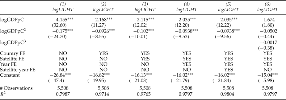
where $\theta_{i} (i = 1,2,{\ldots},I)$ is the time-invariant country fixed effect, μ _{k, t} is the satellite/year/satellite-year fixed effects of satellite $k (k = 1,2{\ldots},K)$ in year $t (t = 1,2,{\ldots},T)$ , and $\epsilon_{i,t}$ is the error term. We refrain from reporting fixed-effects panel data models for two reasons. First, the results obtained from fixed-effects models are nearly identical to the pooled model. Secondly, the overlap of nighttime imagery produced by two different satellites simultaneously allows for a slightly implicit inter-calibration using satellite/satellite-year fixed effects. The model contains 5,508 observations of 181 countries over the period 1992–2013. Estimates of different specifications of the linear model are reported in table 1.

Table 1.

Regression results of general environmental Kuznets curve setup

Notes: t-statistics in parentheses. ***p< 0.001.

In column (1), we perform a simple model by regressing the light figure on the income per capita in linear and quadratic terms. Despite using robust standard errors, both coefficients of income are statistically significant. The coefficient signs are positive for the linear term and negative for the quadratic term and thus imply the expected inverted-U shape. The maximum turning point is located at a per capita income of approximately US$143,000. Column (2) additionally considers country fixed effects, which are important because they serve as a criterion for the level of economic development. This specification yields an R ² of 0.97 and coefficients that are also statistically significant. It is worth noting that the estimated maximum turning point is still a very high level of approximately US$121,000. Columns (3)–(5) add step-by-step satellite, year and satellite-year fixed effects. Consequently, we implicitly control for different satellite-sensor calibrations and technological progress in lighting efficiency. We do not find a noticeable increase in R ², and all estimated coefficients are the same size, implying a maximum turning-point range of US$32,000–51,000. Because this point is exceeded by at least 211 observations, we conclude that the descending part of the EKC indeed exists. As a robustness check, we control for a third-order term of the income measure in column (6). We find that all income coefficients turn insignificant. This result confirms the existence of an inverted-U shape.

Although we aggregate light data on the country level, one could argue that the inverted-U shape is caused by satellite-sensor saturation and is not a consequence of the EKC hypothesis. Although Wu et al. (Reference Wu, Wang, Li and Peng2013) use different light figures, they prove this argument wrong. They exclude observations where saturated areas are more than 0.5 per cent and 0.01 per cent, respectively, but nonetheless find an inverted-U shape. To verify the EKC, the following section provides a different view of the light–income relationship.

4.2. Efficiency

In addition to the traditional EKC perspective, we investigate the ratio of income and lighting to analyze and employ the energy intensity effect, as supposed by Selden et al. (Reference Selden, Forrest and Lockhart1999). According to the EKC hypothesis, environmental degradation depends on the state of economic development and, thus, on the share of each sector in overall production. If the EKC holds, agricultural production and services are less energy and light intensive than manufactural production. To test this assumption, we take a closer look at the logarithmized ratio of income and light (log(GDPpC/LIGHT)). Because this ratio describes the productivity of light, we call this efficiency figure η. η is supposed to be high in countries with a high share of the agricultural sector and/or service sector in GDP, and it will be low if most production is located in manufacturing industries. To test this assumption, we run the following pooled linear regression models:

(2) $$\eta_{i,t} = \gamma_{0}+\gamma_{1}AG_{i,t}+\gamma_{2}SV_{i,t}+\theta_{i}+\mu_{k}+\xi_{t}+\epsilon_{i,t},$$

(3) $$\eta_{i,t} = \delta_{0}+\delta_{1}M_{i,t}+\theta_{i}+\mu_{k}+\xi_{t}+\epsilon_{i,t},$$

where AG _{i, t} is the share of agricultural production in GDP [%] of country $i (i= 1,2,\ldots,I)$ in year $t (t = 1,2,\ldots,T), SV_{i,t}$ is the share of value added by services in GDP [%], M _{i, t} is the percentage of manufacturing in total value added, θ _i is the country fixed effects, μ _k is the satellite fixed effects of satellite $k (k = 1,2\ldots,K), \xi_{t}$ is the year fixed effects and $\epsilon_{i,t}$ is the error term. The equations contain 5050 (2) and 4835 (3) observations, respectively.

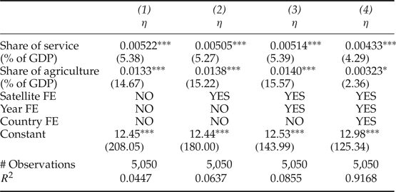
The regression results of equation (2) are reported in table 2. In column (1), we refrain from using any fixed effects and add satellite fixed effects and year fixed effects stepwise in columns (2) and (3). The coefficients of share of service and share of agriculture are both positive, statistically significant and of almost the same magnitude in all three regressions. The interpretation of the coefficients is not straightforward. Because we exclude the share of value added by manufacturing in equation (2), we can say that, e.g., substituting 1 per cent of manufacturing value added by 1 per cent of agricultural value added increases η by 0.014. In column (4), we also control for country fixed effects. The coefficients differ slightly in significance compared with the first three runs. This finding is conclusive because sectoral effects are captured by country fixed effects, and the variation of sector shares within each country is low. Nevertheless, even this setting supports our hypothesis that service and agriculture are more light efficient and thus more CO₂ efficient than manufacturing.

Table 2.

Effect of agriculture and service on η

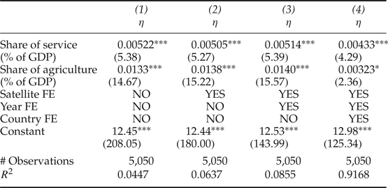
Notes: t-statistics in parentheses. *p< 0.05, ***p< 0.001.

Equation (3) is used as a robustness check of equation (2). The results are reported in table A2 in the online appendix. In all regressions, the coefficient of the share of manufacturing is negative and statistically significant. This finding confirms the results of equation (2).

This analysis of η provides additional evidence for the existence of the EKC in terms of light as a proxy of GHG emissions. It becomes obvious that manufacturing production is comparatively light and thus is emission intensive, whereas agriculture and services are more efficient. However, these results are insufficient to make a statement on the impact of trade on the EKC. Consequently, the following section takes a closer look at trade between high- and low-income countries.

5.1. Effect of trade on η

Due to the different origins of light – either the consumption or production of goods – the effect of trade on η is ambivalent and needs explanation. If trade has no effect on the EKC because the light intensity of imports equals the intensity of exports, we expect, on the one hand, that imports decrease η because pure consumption of imported goods emits light, whereas imports do not increase income. On the other hand, exports are supposed to improve η because income increases, but light caused by consumption is relocated to other countries. Additionally, to avoid problems in interpreting the following results, we focus on imports and exports of merchandise goods and services. To make a statement on the effect of trade, we run the following linear model:

(4) $$\eta_{i,t} = \kappa_{0}+\kappa_{1}{IM}_{i,t}+\kappa_{2}EX_{i,t}+\theta_{i}+\mu_{k}+\xi_{t}+\epsilon_{i,t},$$

where IM _{i, t} is the ratio of merchandise imports to GDP of country $i(i = 1,2,\ldots,I)$ in year $t(t = 1,2,\ldots,T), EX_{i,t}$ is the ratio of merchandise exports to GDP, θ _i are country fixed effects, μ _k is the satellite fixed effects of satellite $k(k = 1,2\ldots,K), \xi_{t}$ are the year fixed effects and $\epsilon_{i,t}$ is the error term.

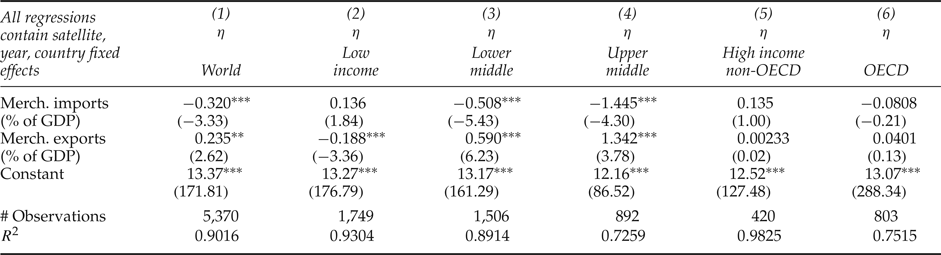
The results of equation (4) can be seen in table 3. In column (1), we take a look at all available observations. The coefficients of imports and exports are both statistically significant and confirm our expectation that trade is neutral. To test the effect of trade on the EKC hypothesis, we divide the sample into five subgroups depending on their World Bank income classification and run the same regression. The results for each subsample are reported in columns (2)–(6). Despite the overall neutral effect, we find evidence that trade has an influence on the EKC. Taking only low-income countries into account, the coefficient's signs are inverted. Because the coefficient of exports is statistically significant and negative, it becomes obvious that low-income countries export goods that are linked with a comparatively light-intensive production. As seen in columns (5) and (6), we do not find a statistically significant coefficient for imports or for exports in high-income countries. This result can also be seen as a lead that high-income countries tend to relocate light- (and carbon-) intensive production and import these goods instead of producing them on their own. Notably, the middle-income countries reported in columns (3) and (4) behave as if trade is neutral. A suitable explanation for this outcome in terms of the EKC is to say that middle-income countries do not need to grow at any price, but they have not yet reached a stage where degradation matters. Thus, their total light or energy trade balance is reasonable.

Table 3.

Effect of trade on η

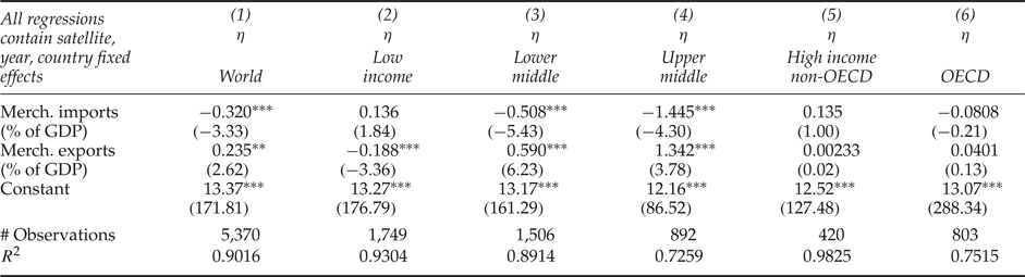
Notes: t-statistics in parentheses. **p< 0.01, ***p< 0.001.

Because the impact of trade on the EKC is a crucial issue, we perform several robustness checks to verify the relationship between trade and η. As a first check, we use the data to estimate a first-differences modelFootnote ² and a fixed-effects model in a similar fashion as that implied by equation (4) to control for additional unobserved effects and/or trends in the data. Therefore, we generate a panel by collapsing the light observations, and we create new satellite configuration dummies. The results of the fixed-effects and first-difference models are reported in tables A3 and A4 in the online appendix. Both models confirm the assumption that trade plays an important role in the discussion of the EKC because the coefficients behave in the expected way even though they are less statistically significant. Furthermore, we run a Dickey–Fuller test with different specifications to control for the stationarity of η. However, all tests reject the null hypothesis that all panels contain unit roots. This result suggests that it can be assumed that η is stationary and ordinary least squares estimates are reasonable. In addition, we split the merchandise import and export variables into their constituents and run the same pooled regressions as in the basic model. The results are reported in table A5 in the online appendix. It becomes obvious that in particular the export of fuel and manufactured goods decreases η in low-income countries. The η of other income categories tends to be positively affected by exports (except exports of agricultural raw materials) if statistically significant coefficients are considered. Furthermore, the import of products such as fuel, manufactured goods and metals is unlikely to change η for the worse in high-income countries. This fact seems to confirm the assumption that high-income countries import goods that come with light-intensive production and refrain from producing them on their own. Thus, the detailed examination of the effect of merchandise imports and exports on η verifies the basic model.

As another robustness check, we generate three new subgroups depending on their income and reexamine the influence of trade on total terms. The first subgroup, called HIGH, contains all observations whose incomes exceed US$40,000, which can be seen as the average maximum turning point of the EKCs calculated in section 4.1. The second subgroup, called MIDDLE, contains observations with incomes between US$5,000 and US$40,000. The last income class, labeled LOW, consists of observations whose incomes are less than US$5,000. Because this classification diverges vastly from the basic model, we can draw robust conclusions on the effect of trade on η if we obtain similar results in the regressions. The results of the diverging subdivisions are reported in table A6 in the online appendix. Despite the broader sample of the LOW category, column (1) shows that the effect of exports is still statistically significant, and it indicates that these countries export goods that come with comparatively light-intensive production. In column (2), we report the regression results for the MIDDLE-income subgroup. This category contains the most observations, and the coefficients behave as if trade is neutral, although they are less significant than in the basic model. Column (3) takes a closer look at HIGH-income countries. Although the HIGH sample consists of only 498 observations, less than half of the high-income sample in the basic model, no trade coefficient is statistically significant. This result is also similar to the basic model. Based on these results, it becomes obvious that the effect of imports and exports on the EKC is not neutral. In addition, we find evidence that high-income countries relocate light-intensive production to low-income countries. However, is it not yet obvious to what extent the traditional inverted-U shape is just caused by trade and the accompanied light and, thus, carbon leakage. We therefore investigate the traditional EKC perspective with respect to trade.

5.2. Effect of trade on the traditional EKC

Because coefficients in regression models reflect ceteris paribus changes, it is not possible to simply add exports and imports to equation (1). Therefore, another approach to examine the traditional EKC is needed. In the previous part of this section, we investigated the effect of merchandise imports and exports on η. In doing so, country fixed effects were included causally, which can now be used to estimate the traditional EKC. The country fixed effects in connection with the constant terms represent the average η of each country during the period of interest on the condition that the share of merchandise imports and exports in GDP equals zero. Thus, we can calculate the average light emissions (ALIGHT) of each country on the condition that there is no merchandise trade, using the average income in the following way:Footnote ³

(5) $${ALIGHT}_{i} = \displaystyle{{AGDPpC}_{i}\over{\displaystyle {e^{\lpar \kappa_{0j} + {CFE}_{i,j}\rpar }}}},$$

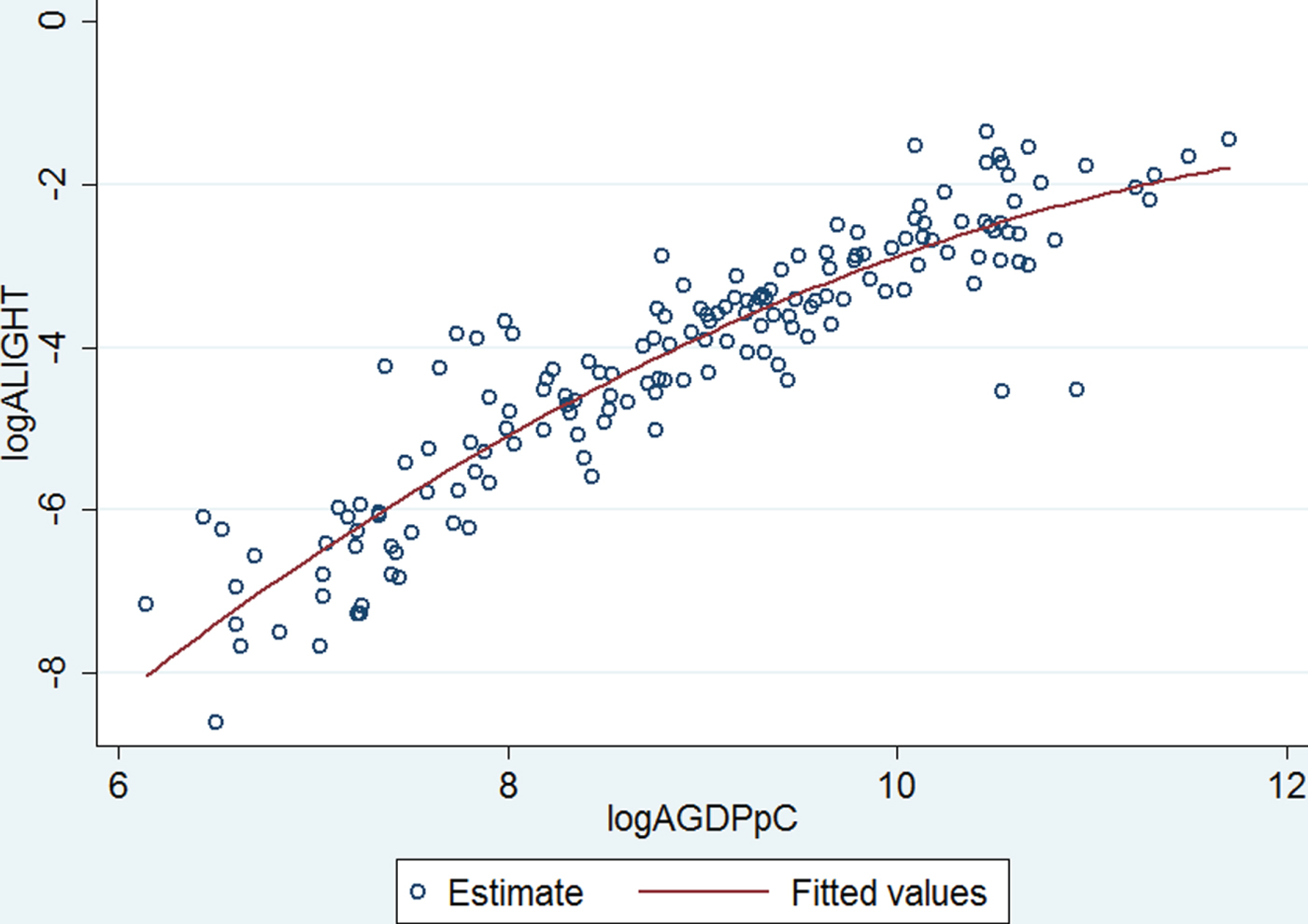
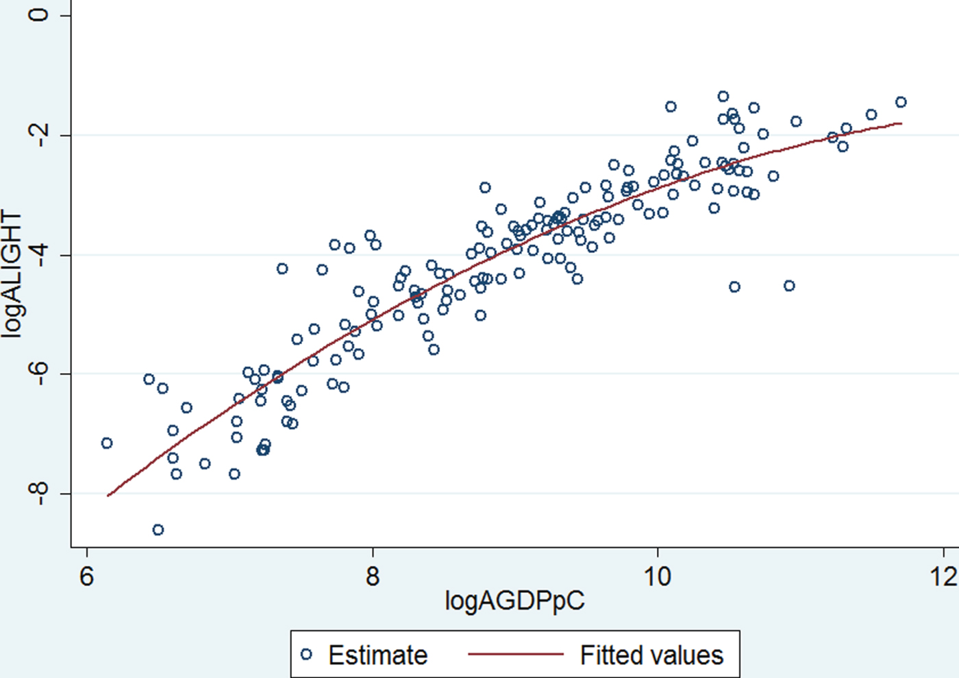
where AGDPpC _i is the average income per capita of country $i (i = 1,2,{\ldots},I), \kappa_{0j}$ is the constant coefficient of the regression of subgroup $j (j = 1,2,{\ldots},J)$ , and is the country fixed effects. A plot of the logarithmized ALIGHT (which is calculated based on the basic model of the previous section) and the logarithmized average income per capita shows that there is a concave curve that is increasing in the range of data (see figure 1). To present a more satisfying statement, we run the following ordinary least squares model:

(6) $$\eqalign{{logALIGHT}_{i} & =\tau_{0}+\tau_{1}{logAGDPpC}_{i}+\tau_{2}{logAGDPpC}_{i}^{2} \cr &\quad +\tau_{3}{logAGDPpC}_{i}^{3}+\epsilon_{i}.}$$

Figure 1.

Light–income relationship conditional on the absence of trade

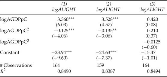
The outcomes of different settings of equation (6) are reported in table 4. In column (1), only the linear and quadratic terms of the average income per capita are taken into account. Both coefficients are statistically significant and point to the expected inverted-U shape. However, it should be mentioned that the absence of trade moves the maximum turning point to an incredibly high level of approximately US$680,000. Due to the fact that the turning point is far beyond the support, it is not reasonable to describe the curve as an inverted-U shape anymore. In fact, it is a concave curve that is increasing in the range of the data. In column (2), we perform the same regression but exclude five countries that have the highest incomes and indicate the beginning of a new upward slope.Footnote ⁴ The regression yields statistically significant coefficients and a maximum turning point of US$470,000, which is far below the turning point estimated in column (1) but is still not exceeded by any observation. In column (3), we test the existence of another upwards slope if these five countries are again included. To do so, the third-order term of income is added in the regression. Because no coefficient is statistically significant, we can conclude that there is no evidence of an N-shape in the data. Furthermore, it can be stated that trade suspends the traditional EKC, because it has a major effect on the location of the maximum turning point. The comparatively good of η high-income countries is primarily caused by relocating light-intensive production.

Table 4.

Traditional environmental Kuznets curve on the condition of the absence of trade

Notes: t−statistics in parentheses. **p<0.01, ***p<0.001.

To verify this finding, we estimate ALIGHT with constants and country fixed effects that result from the more detailed model in the previous section, and we run the same regression as described in equation (6). The results are reported in table A7 in the online appendix and confirm our assumption that trade is not neutral. Notably, the willful neglect of the five highest income observations causes an increase in the maximum turning point income level. Furthermore, in column (3), we find a slightly statistically significant coefficient for the third-order income variable. This finding indicates that there might be an inverted-N shaped relationship between income and light. The inverted-N function has a maximum turning point of less than US$80,000, which is far below the turning points of the trade-restricted inverted-U shapes but still higher than the results calculated in section 4.1.

One could argue that the results are biased because the light figure includes light emitted by the burning of gas flares, and the share of merchandise imports and exports is insufficient to capture this effect. This assumption would imply that the true maximum turning point is located at lower income levels because the light emittance of primarily high-income countries that profit greatly from fossil fuels is overestimated. To disprove this argument, we run regressions of equation (4) considering only observations whose share of fuel exports is less than 15 per cent of all merchandise exports.Footnote ⁵ Then, the outcomes are employed to calculate ALIGHT in the same way as described above and run equation (6) without using the third-order income term. The results of the regression and the attendant diagram can be seen in figure A3 in the online appendix. The omission of these countries does not improve the maximum turning point. Instead, the quadratic term turns insignificant. Because only the linear-income term stays statistically significant, this finding makes the EKC hypothesis implausible. Higher incomes certainly come with intensified light and, thus, higher CO₂ emissions. There is absolutely no downward slope of this curve. Consequently, we can reject the argument of a strongly biased light figure.

Since the EKC relationship is not persistent, we can conclude that trade is a driving force behind the light–income relationship. The worldwide economy has not yet reached a point where the total level of environmental degradation is in decline. Nonetheless, improvements in environmental pollution levels in high-income countries are primarily caused by the relocation of production and the subsequent trade of so-called ‘dirty’ goods.