1 Introduction
Over the years linear stability theory has been the most classical approach applied to understand and describe bifurcations, instability and eventually transition to turbulence in fluid dynamics (Schmid & Henningson Reference Schmid and Henningson2001). It predicts the asymptotic long-term response to small initial perturbations and yields a successful estimation of the critical control parameter where the first bifurcation occurs in many flows (Drazin & Reid Reference Drazin and Reid2004), e.g. Rayleigh–Bénard convection, Taylor–Couette flow between rotating cylinders, or the flow past a cylinder. Nonetheless, some flows exhibit transitions well below the critical Reynolds number
 $Re_{cr}$
predicted by the linear stability analysis: parallel flows, e.g. Couette and Hagen–Poiseuille (Schmid & Henningson Reference Schmid and Henningson2001), as well as non-parallel configurations like jets (Garnaud et al.
Reference Garnaud, Lesshafft, Schmid and Huerre2013) or the flow above a backward-facing step (Barkley, Gomes & Henderson Reference Barkley, Gomes and Henderson2002), among many others.
In Reynolds’ famous pipe flow experiment of 1883 and other examples, the critical Reynolds number of the bifurcation and eventual transition to turbulence is strongly dependent on the level of external noise. This dependence is interpreted by the non-normality of the Navier–Stokes system of equations, which is thus able to amplify perturbations by means of non-modal mechanisms (Trefethen et al. Reference Trefethen, Trefethen, Reddy and Driscoll1993; Chomaz Reference Chomaz2005; Schmid Reference Schmid2007). The non-normality allows the flow to escape from linearly stable solutions by means of large temporal amplification of initial conditions (transient growth) as well as strong response to harmonic forcing, characterized by large gains.
A substantial body of work has therefore been devoted to the understanding of subcritical flows. While modal analysis focusing primarily on eigenvalues cannot predict the bifurcation threshold, other non-modal techniques stemming from classical linear algebra have shed light on the strong amplification potential of linearly stable flows. These techniques determine the optimal perturbations that enforce the largest possible amplification, in other words, the specific perturbation distribution resulting in the maximal transient growth or harmonic gain. Calculations on transient growth have been performed in parallel flows by Butler & Farrell (Reference Butler and Farrell1992), Corbett & Bottaro (Reference Corbett and Bottaro2000) and Schmid (Reference Schmid2007), among others, and in non-parallel two-dimensional (2D) flows by Akervik et al. (Reference Akervik, Ehrenstein, Gallaire and Henningson2008), for spatially developing boundary layers by Alizard, Cherubini & Robinet (Reference Alizard, Cherubini and Robinet2009), Monokrousos et al. (Reference Monokrousos, Akervik, Brandt and Henningson2010) and Sipp & Marquet (Reference Sipp and Marquet2012) and for the backward-facing step by Blackburn, Barkley & Sherwin (Reference Blackburn, Barkley and Sherwin2008), among others. Optimal harmonic forcing structures that produce the largest amplifications in response (Farrell & Ioannou Reference Farrell and Ioannou1996; Schmid Reference Schmid2007) have been studied for instance in parallel plane Couette applying wavenumber expansion by Jovanović & Bamieh (Reference Jovanović and Bamieh2005). For several spatially developing open flows, Akervik et al. (Reference Akervik, Ehrenstein, Gallaire and Henningson2008), Alizard et al. (Reference Alizard, Cherubini and Robinet2009) and Sipp & Marquet (Reference Sipp and Marquet2012) have determined the optimal harmonic gain curves, which systematically displayed a preferred frequency. The harmonic response of the shear layer shed by the corner of the 2D backward-facing step was then determined by Marquet & Sipp (Reference Marquet and Sipp2010) and later by Boujo & Gallaire (Reference Boujo and Gallaire2015), among others.
A related but different approach is the study of the response to white noise, as was introduced for parallel flows by Farrell & Ioannou (Reference Farrell and Ioannou1993). For non-parallel flows, Dergham, Sipp & Robinet (Reference Dergham, Sipp and Robinet2013) present a low-dimensional model to approximate the linear response of white noise for the 2D backward-facing step, while Boujo & Gallaire (Reference Boujo and Gallaire2015) study the sensitivity and control of the response amplification under stochastic forcing. Whilst most of the non-modal studies presented rely on the linearization around the stable steady solution of the Navier–Stokes equations (NSEs), defined as base flow, an attempt to describe more precisely the actual physics involved in the strong noise amplification exhibited in turbulent jets has been pursued by Garnaud et al. (Reference Garnaud, Lesshafft, Schmid and Huerre2013), who applied the optimal gain analysis on a model mean flow for globally stable jets.
All these studies rely on the linear response to perturbations, either intrinsic (instability) or externally driven (forcing), and are not able to describe saturation processes or the nonlinear interaction existing between the mean flow and fluctuating coherent structures, thus driving the need of characterizing the nonlinear effects involved. A well-known description of the physical mechanism that takes place in the saturation of a supercritical instability close to threshold is presented by the Stuart–Landau amplitude equation introduced back in the 1960s (Stuart Reference Stuart1960). This description arises from an earlier attempt (Stuart Reference Stuart1958) to capture the saturation mechanism introducing the mean flow modification through the Reynolds stress constructed by the most unstable eigenmode. With similar nonlinear ideas, a 2D three-velocity-component (2D/3C) model was proposed recently for turbulence in plane Couette flow (Gayme et al. Reference Gayme, McKEON, Papachristodoulou, Bamieh and Doyle2010). The model supports a one-way coupling where the mean flow is influenced by the perturbation field, but not vice versa. Other models where a two-way coupling is applied are for example the stochastic structural stability theory (SSST) proposed by Farrell & Ioannou (Reference Farrell and Ioannou2003). It consists in writing the linear response to white noise forcing in the form of a Lyapunov equation, and coupling it to the ensemble-average mean flow by means of the Reynolds stress. The theory is able to describe the appearance of large coherent fluctuating structures in turbulent atmospheric flows (Farrell & Ioannou Reference Farrell and Ioannou2003), as well as in the three-dimensional (3D) Couette flow (Farrell & Ioannou Reference Farrell and Ioannou2012), all of them being linearly stable. Other models with a linear perturbation equation coupled to the mean flow have been proposed to describe the coherent structures appearing in the transition to turbulence for parallel shear flow, as in Beaume et al. (Reference Beaume, Chini, Julien and Knobloch2015), or the restricted nonlinear (RNL) model introduced in Thomas et al. (Reference Thomas, Lieu, Jovanović, Farrell, Ioannou and Gayme2014).
In the spirit of these studies, where a closed coupling is present between a linear perturbation equation and the mean flow, we propose herein a model that describes the nonlinear saturation of the response to sustained harmonic forcing for laminar stable flows. The response to forcing in unstable unsteady flows is not included in the present study, as it implies a more involved approach accounting jointly for the unstable terms together with the response to the forcing, as described in Lu & Papadakis (Reference Lu and Papadakis2011). The introduced model relates to that recently proposed for unstable laminar flows in Mantič-Lugo, Arratia & Gallaire (Reference Mantič-Lugo, Arratia and Gallaire2014, Reference Mantič-Lugo, Arratia and Gallaire2015) and applied to the nonlinear saturation in the cylinder flow. The model is specifically applied to the well known backward-facing step case study in 2D at
 $Re=500$
. It is globally stable since the first bifurcation is a 3D global instability at
 $Re_{cr}\sim 748$
(Barkley et al.
Reference Barkley, Gomes and Henderson2002; Lanzerstorfer & Kuhlmann Reference Lanzerstorfer and Kuhlmann2012). First, a weakly nonlinear asymptotic expansion is developed around the stable base flow, showing the Reynolds stress as the key nonlinear term in the saturation process. Its range of validity is however seen to be limited to very small forcing amplitudes. In contrast, the linear response around the mean flow computed by direct numerical simulation (DNS) captures very well the nonlinear saturation at larger forcing amplitude. However, in this approach the equations are decoupled and solved a posteriori. This motivates the introduction of the self-consistent model, which is solved a priori and where the mean flow is strongly coupled with the linear response to harmonic forcing by means of the Reynolds stress and the higher harmonic generation is neglected. The model presents an accurate prediction of the saturation as much as of the structure of the response and mean flow. It highlights the importance of the Reynolds stress in the nonlinear saturation process, similarly to the unstable cylinder flow, as already discussed by Barkley (Reference Barkley2006), Mittal (Reference Mittal2008) and Turton, Tuckerman & Barkley (Reference Turton, Tuckerman and Barkley2015), among others.
The paper is organized as follows. In § 2 the flow configuration is described and the numerical method is explained. Section 3 presents the classical linear response calculation and reveals the difference with the harmonically forced DNS results. Section 4 presents the linear response around the mean flow that motivates the self-consistent model described in § 5. Finally the results of the model are compared to the exact DNS in § 5.2 and the conclusions are summarized in § 6.
2 Problem formulation
2.1 Flow geometry and governing equations
The case study selected is the 2D incompressible laminar flow around the backward-facing step. The configuration is sketched in figure 1. It consists of an inlet channel of height
 $h$
and length
 $L_{i}=5h$
followed by a step of height
 $h$
entailing a sudden expansion of height
 $H$
, where
 $H=2h$
, hence the expansion ratio is
 ${\it\Gamma}=h/H=0.5$
as depicted in figure 1. The Reynolds number is defined as
 $Re=hU_{\infty }/{\it\nu}$
, where
 $h$
is the inlet channel height,
 $U_{\infty }$
the centreline (maximum) velocity of the plane Poiseuille inlet boundary condition and
 ${\it\nu}$
the kinematic viscosity. The non-dimensionalized frequency defined by the Strouhal number is given by
 $St=fh/(U_{\infty })={\it\omega}/(2{\rm\pi})$
. Throughout the article, all the variables are non-dimensional using length
 $h$
, density
 ${\it\rho}_{\infty }$
and velocity
 $U_{\infty }$
as reference scales.
Sketch of the flow configuration superimposed onto the velocity field in the
 $x$
direction of the base flow for the backward-facing step at
 $Re=500$
.

The flow is governed by the forced 2D incompressible NSEs,
 $$\begin{eqnarray}\partial _{t}\boldsymbol{u}+\mathscr{N}(\boldsymbol{u})=\boldsymbol{f},\end{eqnarray}$$
where
 $$\begin{eqnarray}\mathscr{N}(\boldsymbol{u})\equiv (\boldsymbol{u}\boldsymbol{\cdot }\boldsymbol{{\rm\nabla}})\boldsymbol{u}+\boldsymbol{{\rm\nabla}}p-Re^{-1}{\rm\Delta}\boldsymbol{u}\end{eqnarray}$$
corresponds to the advective, pressure gradient and diffusive terms. In the entire study, the pressure field
 $p$
is such that velocity fields are divergence-free
 $\boldsymbol{{\rm\nabla}}\boldsymbol{\cdot }\boldsymbol{u}=0$
following the incompressibility condition. The term
 $\boldsymbol{f}$
represents a harmonic body forcing of the form
 $\boldsymbol{f}(\boldsymbol{x},t)=\boldsymbol{f}_{1}(\boldsymbol{x})\text{e}^{\text{i}{\it\omega}t}+\text{c.c.}$
with a given fixed frequency
 $St={\it\omega}/(2{\rm\pi})$
.
2.2 Linear transfer function
The steady solution of the NSEs,
 $$\begin{eqnarray}\mathscr{N}(\boldsymbol{U}_{B})=0,\end{eqnarray}$$
is called the base flow
 $\boldsymbol{U}_{B}$
and is linearly stable for the 2D backward-facing step with expansion ratio
 ${\it\Gamma}=0.5$
at the chosen
 $Re=500$
, with its first unstable mode appearing in 3D for
 $Re_{cr}\sim 748$
(Barkley et al.
Reference Barkley, Gomes and Henderson2002; Lanzerstorfer & Kuhlmann Reference Lanzerstorfer and Kuhlmann2012). The classical approach is to study the linear response to harmonic forcing around this stable base flow. Figure 1 shows the outline of the base flow of the backward-facing step at
 $Re=500$
.
The exact nonlinear response can be approximated by the linear response, assuming a small amplitude of the harmonic forcing,
 $$\begin{eqnarray}[\partial _{t}\boldsymbol{u}_{1B}^{\prime }+\mathscr{L}_{\boldsymbol{ U}_{B}}(\boldsymbol{u}_{1B}^{\prime })]=\boldsymbol{f},\end{eqnarray}$$
where higher-order nonlinear terms are neglected as a first approximation, and the general operator
 $\mathscr{L}_{\boldsymbol{U}}(\boldsymbol{u}^{\prime })$
is the corresponding operator for the NSEs linearized around any
 $\boldsymbol{U}$
, i.e.
 $$\begin{eqnarray}\mathscr{L}_{\boldsymbol{U}}(\boldsymbol{u}^{\prime })\equiv (\boldsymbol{U}\boldsymbol{\cdot }\boldsymbol{{\rm\nabla}})\boldsymbol{u}^{\prime }+(\boldsymbol{u}^{\prime }\boldsymbol{\cdot }\boldsymbol{{\rm\nabla}})\boldsymbol{U}+\boldsymbol{{\rm\nabla}}p^{\prime }-Re^{-1}{\rm\Delta}\boldsymbol{u}^{\prime }.\end{eqnarray}$$
Furthermore, since the forcing is harmonic, the corresponding response
 $\boldsymbol{u}^{\prime }(\boldsymbol{x},t)$
will also be harmonic,
 $\boldsymbol{u}^{\prime }(\boldsymbol{x},t)\simeq \boldsymbol{u}_{1B}^{\prime }(\boldsymbol{x},t)=\boldsymbol{u}_{1B}(\boldsymbol{x})\text{e}^{\text{i}{\it\omega}t}+\text{c.c.}$
, and oscillate purely at the forcing frequency, due to the linearity of the operator (2.4).
The linear equation (2.4) can be rewritten formally as
 $\boldsymbol{u}_{1B}=\mathscr{R}({\it\omega})\boldsymbol{f}_{1}$
, where
 $\mathscr{R({\it\omega})}=(\text{i}{\it\omega}+\mathscr{L}_{\boldsymbol{U}})^{-1}$
is the resolvent operator. The amplitude of the response in general can be measured as the square root of the kinetic energy of the purely time-dependent fluctuation averaged over one period
 $T$
,
 $$\begin{eqnarray}R=\sqrt{\frac{1}{T}\int _{0}^{T}\!\int _{{\it\Omega}}\boldsymbol{u}^{\prime 2}\,\text{d}{\it\Omega}}\,\text{d}t.\end{eqnarray}$$
Consequently, the amplitude of the linear response
 $\boldsymbol{u}_{1B}^{\prime }$
corresponds to the
 $L^{2}$
norm
 $$\begin{eqnarray}R=\sqrt{\frac{1}{T}\int _{0}^{T}\!\int _{{\it\Omega}}\boldsymbol{u}_{1B}^{\prime 2}\,\text{d}{\it\Omega}\,\text{d}t}=\sqrt{2}\Vert \boldsymbol{u}_{1B}\Vert ,\end{eqnarray}$$
as it is sinusoidal in time, defining the
 $L^{2}$
norm as determined by the Hermitian inner product
 $(\boldsymbol{a}\mid \boldsymbol{b})=\int _{{\it\Omega}}\overline{\boldsymbol{a}}\boldsymbol{\cdot }\boldsymbol{b}\,\text{d}{\it\Omega}$
, for complex fields in the domain
 ${\it\Omega}$
. In the same fashion, the forcing amplitude is calculated as the
 $L^{2}$
norm of the harmonic forcing,
 $$\begin{eqnarray}A=\sqrt{\frac{1}{T}\int _{0}^{T}\!\int _{{\it\Omega}}\boldsymbol{f}^{2}\,\text{d}{\it\Omega}\,\text{d}t}=\sqrt{2}\Vert \,\boldsymbol{f}_{1}\Vert .\end{eqnarray}$$
A natural way of measuring the amplification is the gain,
 $$\begin{eqnarray}G({\it\omega})=R/A,\end{eqnarray}$$
which is defined as the ratio between the amplitude of the response to the amplitude of the input. Subsequently, for the linear case of harmonic forcing, it reads
 $$\begin{eqnarray}G({\it\omega})=\Vert \boldsymbol{u}_{1B}\Vert /\Vert \,\boldsymbol{f}_{1}\Vert .\end{eqnarray}$$
In particular, it is relevant to determine the largest energy amplification possible at a given frequency, or in other words the optimal gain
 $G_{opt}({\it\omega})$
that is associated to the optimal forcing
 $\boldsymbol{f}_{opt}$
,
 $$\begin{eqnarray}G_{opt}({\it\omega})=\max _{\boldsymbol{f}_{1}}\frac{\Vert \boldsymbol{u}_{1B}\Vert }{\Vert \,\boldsymbol{f}_{1}\Vert }=\frac{\Vert \mathscr{R}({\it\omega})\boldsymbol{f}_{opt}\Vert }{\Vert \,\boldsymbol{f}_{opt}\Vert }.\end{eqnarray}$$
Introducing the adjoint of the resolvent operator, the gain can be rewritten as a Rayleigh quotient of the resolvent operator and the forcing,
 $$\begin{eqnarray}G^{2}({\it\omega})=\frac{(\mathscr{R}\boldsymbol{f}_{1}\mid \mathscr{R}\boldsymbol{f}_{1})}{(\boldsymbol{f}_{1}\mid \boldsymbol{f}_{1})}=\frac{(\mathscr{R}^{H}\mathscr{R}\boldsymbol{f}_{1}\mid \boldsymbol{f}_{1})}{(\boldsymbol{f}_{1}\mid \boldsymbol{f}_{1})}.\end{eqnarray}$$
Subsequently, the optimal gain and forcing correspond to the leading eigenvalue
 ${\it\lambda}_{1}=G_{1}^{2}$
and eigenvector
 $\hat{\boldsymbol{f}}_{1}$
of the symmetric eigenvalue problem
 $\mathscr{R}^{H}\mathscr{R}\hat{\boldsymbol{f}}_{k}={\it\lambda}_{k}\hat{\boldsymbol{f}}_{k}$
. The procedure undertaken to obtain the optimal gain is described in more detail in Garnaud et al. (Reference Garnaud, Lesshafft, Schmid and Huerre2013) and Boujo & Gallaire (Reference Boujo and Gallaire2015). Thus, we obtain for each forcing frequency an optimal forcing spatial distribution with its associated gain. A comparison of the optimal gains at different frequencies enables us to obtain the overall optimal gain
 $G_{opt}$
with its corresponding forcing
 $\boldsymbol{f}_{opt}$
. Notice that this optimization is achieved only for the linear equation, and not for the full nonlinear gain of the DNS.
2.3 Numerical methods
The linear and nonlinear NSEs are solved by applying the finite element method representing the spatial discretization of the flow fields
 $(u_{x},u_{y},p)$
by Taylor–Hood (P2, P2, P1) elements. The software FreeFEM++ is used to generate the domain
 ${\it\Omega}$
triangulation and to build all the required operators. The linear operators are solved by a sparse solver implemented directly in FreeFEM++, while the singular value decomposition is solved in Matlab. The nonlinear systems as the steady-state solutions are solved by the iterative Newton–Raphson method. The time integration of the DNS of the NSEs is calculated by applying a time scheme based on the characteristics–Galerkin method as described in Benitez & Bermudez (Reference Benitez and Bermudez2011).
The computational domain under consideration is defined in Cartesian coordinates with the origin at the step edge. The nominal domain spans from
 $x=-5h$
to
 $x=50h$
with an inlet
 $y=(0,h)$
and an outlet
 $y=(-h,h)$
as depicted in figure 1, being the same size as in Boujo & Gallaire (Reference Boujo and Gallaire2015). A 2D plane Poiseuille profile is imposed as the inlet Dirichlet boundary condition
 $x_{i}=-h$
. No-slip conditions are imposed at the upper
 $y=h$
and lower
 $y=-h$
boundary and an outflow boundary condition is imposed at the outlet
 $x_{o}=50h$
.
The size of the domain was chosen after thorough validation. The length of the domain is selected such that the base flow outlet profile returns to the fully developed Poiseuille profile, presenting a relative error between the base flow and the parabolic profile of less than 1 % in
 $L^{2}$
and
 $L_{\infty }$
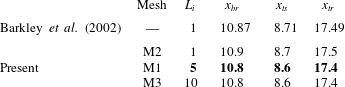
norm. The influence of the entrance length on the recirculation bubble is summarized in table 1 and compared to Barkley et al. (Reference Barkley, Gomes and Henderson2002), to ensure that the chosen length is large enough and the solutions obtained are general and independent of further increase in domain size. In addition, the length of the recirculation bubble shows an excellent match for the whole range of Reynolds number compared to Barkley et al. (Reference Barkley, Gomes and Henderson2002) and Blackburn et al. (Reference Blackburn, Barkley and Sherwin2008).
Comparison of the recirculation bubble position for different domain geometries, i.e. variation of inlet length
 $L_{i}$
. The selected domain and mesh is marked in bold.

The nominal domain and mesh M1 is of 33 814 cells and 155 691 degrees of freedom (DoF), giving a gain of 7453 represented in bold in table 2, which compares quantitatively well to the optimal
 $G_{opt}=7480$
computed by Marquet & Sipp (Reference Marquet and Sipp2010) ensuring the quality of the methodology and mesh used. Furthermore, mesh independence is verified by doubling the number of cells by a uniform refinement, obtaining M6 with 338 247 DoF and 73 982 cells, which provides a gain of 7456, thus a relative variation of less than 0.05 %.
Comparison of the linear optimal gain at
 $St=0.075$
for different domain geometries. The selected domain and mesh is marked in bold.

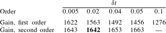
First- and second-order methods (Benitez & Bermudez Reference Benitez and Bermudez2011) are compared for the time integration scheme of the DNS in table 3. The second-order method is chosen, as it presents much more robust results in terms of gain when compared to the first-order method in spite of a small increase in the computational time. The DNS time step is chosen by achieving time-step-independent results in terms of nonlinear gain as summarized in table 3. The selected time step
 ${\it\delta}t=0.02$
is deemed to be small enough as a trade-off between accuracy and computational time since it is located in the time-step-independent region.
Nonlinear saturated gain
 $G$
of the DNS for different time steps
 ${\it\delta}t$
. The nonlinear solution is forced by the optimal harmonic forcing of amplitude
 $A=4\times 10^{-4}$
for
 $Re=500$
. The selected time scheme is second order and the time step is
 ${\it\delta}t=0.02$
marked in bold.

3 Linear and nonlinear response to harmonic forcing
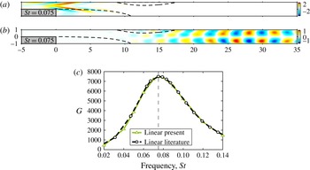
Applying the linear formulation described in § 2.2 to the 2D backward-facing step flow, the optimal forcing and response are calculated. The associated optimal gain obtained around the base flow is very large, with an overall optimal gain of
 $G_{opt}=7480$
at
 $Re=500$
, obtained for a non-dimensional frequency of
 $St=0.075$
, the same as that reported by Marquet & Sipp (Reference Marquet and Sipp2010) and Boujo & Gallaire (Reference Boujo and Gallaire2015), see figure 2. This optimal forcing at
 $St=0.075$
will be used throughout the paper, and unless stated otherwise
 $\boldsymbol{f}_{1}=\boldsymbol{f}_{opt}$
, although the methodology is independent of the shape and frequency of the forcing and any body or boundary harmonic forcing could be used.
(a) Linear optimal forcing in the
 $x$
direction and (b) linear optimal response in the
 $x$
direction at overall optimal frequency
 $St=0.075$
. (c) Linear optimal gain at each forcing frequency
 $St$
; comparison to Marquet & Sipp (Reference Marquet and Sipp2010). All results at
 $Re=500$
.

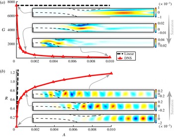
The large optimal gain implies that linear prediction has a small region of validity since the nonlinear effects enter at small forcing amplitudes
 $A$
, as illustrated in figure 3(a), where the nonlinear gain decreases rapidly with an increase of the forcing amplitude. This effect is exacerbated because the chosen forcing is optimal
 $\boldsymbol{f}_{1}=\boldsymbol{f}_{opt}$
for the sake of generality and presents a complex structure (figure 2) that can be attained only numerically. Therefore, in any real experiment the forcing would project poorly on the optimal, yielding a much weaker linear gain and thus requiring larger forcing amplitude
 $A$
to achieve such nonlinear saturation. However, the procedure presented in this paper is general and can be applied to any forcing structure, including body or boundary forcing.
The same saturation process is represented differently through the response amplitude in figure 3(b) defined as the square root of the energy of the fluctuation. Note how the strong saturation of the DNS response for large forcing amplitudes
 $A$
entails a discrepancy of orders of magnitude as compared to the linear response. The insets in figure 3(b) show snapshots of the fluctuating velocity at different forcing amplitudes. The energy maximum of the response experiences a clear migration upstream during the saturation process, reducing the mean recirculation bubble. A similar tendency has been previously encountered in the cylinder flow and described by Zielinska et al. (Reference Zielinska, Goujon-Durand, Dusek and Wesfreid1997). This migration is enforced by the modification of the base flow into the mean flow due to the forcing of the Reynolds stress as described by Barkley (Reference Barkley2006) and thoroughly examined in Mantič-Lugo et al. (Reference Mantič-Lugo, Arratia and Gallaire2014). Figure 3(a) illustrates how the Reynolds stress forcing also moves upstream with an increase in harmonic forcing amplitude
 $A$
along with the modifications of the response that creates it. In other words, increasingly stronger harmonic forcing entails stronger response, which in turn creates stronger Reynolds stresses that modify the mean flow and yield saturation, which reduces the response in comparison to its linear prediction.
(a) Gain and (b) response of the linear prediction around the base flow compared to the nonlinear saturated DNS for the optimal forcing at
 $St=0.075$
and
 $Re=500$
. The insets in (a) show the Reynolds stress divergence in the
 $x$
direction and the insets in (b) show the response, or, in other words, the pure fluctuating velocity
 $\boldsymbol{u}^{\prime }$
, in the
 $y$
direction.

4 Linear response around mean flow
As a starting point, we introduce an asymptotic expansion in an attempt to capture the mechanism that governs the saturation of the response where the classical linear approach fails (figure 3). The asymptotic expansion is carried out around the base flow
 $\boldsymbol{U}_{B}$
plus the perturbation, being the harmonic fluctuation at different orders
 $\boldsymbol{u}=\sum _{n=0}^{\infty }\sum _{p=0}^{\infty }{\it\epsilon}^{n}\boldsymbol{u}_{p,n}\text{e}^{\text{i}p{\it\omega}t}$
, with a small parameter
 ${\it\epsilon}=A$
corresponding to the amplitude of the forcing. The expansion is stopped at third order
 ${\it\epsilon}^{3}$
and the influence of the different terms in the weakly nonlinear gain is analysed. More details are given in the appendix A for the sake of clarity.
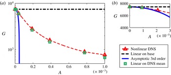
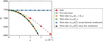
The results agree with the DNS close to the threshold, as seen in figure 4, and suggest that qualitatively the nonlinear saturation process is dominated by the Reynolds stress modification and not by the higher harmonics interaction. This analysis highlights the importance of the mean flow, as in many cases reported in the literature, where linear stability analysis applied to the mean flows predicted the accurate frequency and structure of the fluctuations, e.g. the cylinder flow (Barkley Reference Barkley2006). However, the asymptotic analysis does not provide a quantitative prediction since the region of validity is extremely limited.
Subsequently a natural step is to address the linear response around the mean flow far from threshold. We introduce the Reynolds decomposition given by
 $\boldsymbol{u}(\boldsymbol{x},t)=\boldsymbol{U}(\boldsymbol{x})+\boldsymbol{u}^{\prime }(\boldsymbol{x},t)=\boldsymbol{U}_{B}(\boldsymbol{x})+{\rm\Delta}\boldsymbol{U}(\boldsymbol{x})+\boldsymbol{u}^{\prime }(\boldsymbol{x},t)$
. The instantaneous flow is expressed as a mean flow
 $\boldsymbol{U}=\langle \boldsymbol{u}\rangle$
plus a pure fluctuation
 $\boldsymbol{u}^{\prime }$
verifying
 $\langle \boldsymbol{u}^{\prime }\rangle =0$
, where
 $\langle \,\rangle$
denotes time averaging and
 ${\rm\Delta}\boldsymbol{U}$
corresponds to the base flow modification. Substituting the Reynolds decomposition in the full NSEs we obtain a set of two coupled equations:
 $$\begin{eqnarray}\displaystyle & \displaystyle \mathscr{N}(\boldsymbol{U})=-\langle (\boldsymbol{u}^{\prime }\boldsymbol{\cdot }\boldsymbol{{\rm\nabla}})\boldsymbol{u}^{\prime }\rangle , & \displaystyle\end{eqnarray}$$
 $$\begin{eqnarray}\displaystyle & \displaystyle \partial _{t}\boldsymbol{u}^{\prime }+\mathscr{L}_{\boldsymbol{U}}(\boldsymbol{u}^{\prime })=-(\boldsymbol{u}^{\prime }\boldsymbol{\cdot }\boldsymbol{{\rm\nabla}})\boldsymbol{u}^{\prime }+\langle (\boldsymbol{u}^{\prime }\boldsymbol{\cdot }\boldsymbol{{\rm\nabla}})\boldsymbol{u}^{\prime }\rangle +\boldsymbol{f}. & \displaystyle\end{eqnarray}$$
 $\boldsymbol{U}$
arises as a result of the steady mean flow equation (4.1a
) while the perturbation or forced response equation (4.1b
) governs the time-dependent field
 $\boldsymbol{u}^{\prime }$
. Through this decomposition, it is possible to easily isolate two significant nonlinear terms of the fluctuation interacting with itself. First, the right-hand side of (4.1a
) corresponds to the Reynolds stress forcing
 $\langle (\boldsymbol{u}^{\prime }\boldsymbol{\cdot }\boldsymbol{{\rm\nabla}})\boldsymbol{u}^{\prime }\rangle$
, a mean momentum addition to
 $\boldsymbol{U}$
due to the nonlinear interaction of the time-dependent fluctuation
 $\boldsymbol{u}^{\prime }$
. Second, the nonlinear right-hand side of (4.1b
),
 $(\boldsymbol{u}^{\prime }\boldsymbol{\cdot }\boldsymbol{{\rm\nabla}})\boldsymbol{u}^{\prime }-\langle (\boldsymbol{u}^{\prime }\boldsymbol{\cdot }\boldsymbol{{\rm\nabla}})\boldsymbol{u}^{\prime }\rangle$
, represents the time-dependent, zero-mean, momentum addition from the nonlinear interactions of different harmonics in
 $\boldsymbol{u}^{\prime }$
. Note that the coupled equations are exact, as no simplification was made at this stage, and the time-dependent perturbation
 $\boldsymbol{u}^{\prime }$
does not have to be small compared to the mean
 $\boldsymbol{U}$
.
Gain saturation as a function of the forcing amplitude
 $A$
for DNS (triangles) compared to the asymptotic solution (solid line) and linear response
 $\boldsymbol{u}_{1DNS}$
around the saturated mean flow from DNS (squares). Forcing with optimal structure at frequency
 $St=0.075$
and
 $Re=500$
.

Equation (4.1b ) is linearized neglecting the interaction of the higher harmonics gathered on its right-hand side, yielding
 $$\begin{eqnarray}[\partial _{t}\boldsymbol{u}_{1}^{\prime }+\mathscr{L}_{\boldsymbol{ U}_{DNS}}(\boldsymbol{u}_{1}^{\prime })]=\boldsymbol{f},\end{eqnarray}$$
a linear equation equivalent to (2.4) around the mean flow
 $\boldsymbol{U}_{DNS}$
extracted from DNS, instead of the base flow
 $\boldsymbol{U}_{B}$
. At each forcing amplitude
 $A$
, the mean flow has to be calculated since the Reynolds stress forcing term on the right-hand side of (4.1a
) changes in structure and amplitude. The solution to (4.2) corresponds to a single harmonic response oscillating at the forcing frequency
 ${\it\omega}$
.
The linear response to harmonic forcing around the mean flow provides a very good prediction of the nonlinear gain as shown in figure 4. This results are in line with the results of stability analyses around mean flows performed in the literature (see Barkley Reference Barkley2006, among others) since (4.2) corresponds to the forcing counterpart of an eigenvalue problem in stability analyses.
Extracting the different harmonics of the nonlinear DNS response
 $\boldsymbol{u}^{\prime }(\boldsymbol{x},t)$
by Fourier series, we have indeed obtained an energy of the second harmonic less than 3 % of the fundamental frequency for a forcing amplitude
 $A=0.01$
. Therefore, the fluctuating response signal
 $\boldsymbol{u}^{\prime }(\boldsymbol{x},t)$
is dominated by the first harmonic even for a strongly saturated DNS, and, as recently interpreted in Turton et al. (Reference Turton, Tuckerman and Barkley2015) for an unstable flow, quasi-monochromatic flows seem to be well predicted by a linearization around their temporal mean.
In a similar spirit, the first harmonic approximation of a nonlinear response has been recently used for the description of combustion instabilities, where Noiray et al. (Reference Noiray, Durox, Schuller and Candel2008) have applied the concept of describing function (i.e. a nonlinear extension of the linear transfer function) to flames.
5 Self-consistent model
The linear response around the mean flow might appear as somewhat inconsistent, since it results from a decoupled system of equations, where the Reynolds stress is computed from the full nonlinear fluctuation that is obtained a posteriori from DNS or experiments (4.1a
), and does not correspond to the linear fluctuation from (4.2). Notice that also the weakly nonlinear solution (appendix A) arises from only partially coupled equations up to third order, which are solved one after the other, sequentially, thus suggesting an explanation for its limitation to small forcing amplitude
 $A={\it\epsilon}$
. These limitations are overcome in the present semi-linear model by coupling the nonlinear mean flow and the linear perturbation equation. The model consists of the full instantaneous response approximated by a single harmonic
 $\boldsymbol{u}(\boldsymbol{x},t)=\boldsymbol{U}(\boldsymbol{x})+\boldsymbol{u}^{\prime }(\boldsymbol{x},t)\simeq \boldsymbol{U}(\boldsymbol{x})+\boldsymbol{u}_{1}^{\prime }(\boldsymbol{x},t)$
, for
 $\boldsymbol{u}_{1}^{\prime }(\boldsymbol{x},t)=\boldsymbol{u}_{1}(\boldsymbol{x})\text{e}^{\text{i}{\it\omega}t}+\text{c.c.}$
, coupled to the mean flow equation by the Reynolds stress forcing. In addition, the mean flow is obtained a priori and it is not extracted from DNS or experimental values but given from (4.1a
) with the fluctuation from the linear response around the aforementioned mean flow, forming a closed system of interactions. The coupled equations of the self-consistent model for harmonically forced flows can be written as
 $$\begin{eqnarray}\displaystyle & \displaystyle \mathscr{N}(\boldsymbol{U})=-2\,\text{Re}((\bar{\boldsymbol{u}}_{1}\boldsymbol{\cdot }\boldsymbol{{\rm\nabla}})\boldsymbol{u}_{1}), & \displaystyle\end{eqnarray}$$
 $$\begin{eqnarray}\displaystyle & \displaystyle \text{i}{\it\omega}\boldsymbol{u}_{1}+\mathscr{L}_{\boldsymbol{U}}(\boldsymbol{u}_{1})=\boldsymbol{f}_{1}, & \displaystyle\end{eqnarray}$$
 $\mathscr{R({\it\omega})}=(\text{i}{\it\omega}+\mathscr{L}_{\boldsymbol{U}})^{-1}$
and ultimately the gain. The fluctuation velocity fields
 $\boldsymbol{u}_{1}$
are divergence-free as well as the mean flow
 $\boldsymbol{U}$
and the overline
 $\overline{(.)}$
means complex conjugate.
Conceptually the model is the forced counterpart for amplifiers of the self-consistent model presented recently for oscillators (Mantič-Lugo et al. Reference Mantič-Lugo, Arratia and Gallaire2014, Reference Mantič-Lugo, Arratia and Gallaire2015) where the linear equation corresponded to an eigenvalue problem and the amplitude was dictated by the marginality criterion of the system. Similarly, in the model introduced by Beaume et al. (Reference Beaume, Chini, Julien and Knobloch2015), the fluctuations are equally treated linearly corresponding to an eigenvalue problem with the amplitude of the fluctuation enforced by the marginal stability criterion. Nonetheless, in this case the flow is asymptotically stable: the turbulent plane Couette flow. The self-consistent model proposed herein also relates closely to the SSST theory (Farrell & Ioannou Reference Farrell and Ioannou2012) and the RNL model (Thomas et al. Reference Thomas, Lieu, Jovanović, Farrell, Ioannou and Gayme2014), all for turbulent flows, where the linear response to white noise forcing is coupled to the mean flow modification through the Reynolds stress. However, in the present case the forcing is harmonic and not uncorrelated like the white noise in SSST, thus the linear response to forcing can be used and the Lyapunov equation is not required. Furthermore, the semi-linear model assumes a steady saturated mean flow while the SSST theory is characterized by a slowly varying ensemble-averaged mean flow. The self-consistent model as described in (5.1) is expected to work for stable laminar flows with a quasi-monochromatic response to forcing, while the model introduced recently in Mantič-Lugo et al. (Reference Mantič-Lugo, Arratia and Gallaire2014, Reference Mantič-Lugo, Arratia and Gallaire2015) is proposed for unstable laminar flows with quasi-monochromatic instability (Turton et al. Reference Turton, Tuckerman and Barkley2015). It presents a simplified and more transparent system than the DNS since the different terms are isolated, while still capturing the saturation process for stable or unstable laminar flows.
5.1 Model solution
The coupled equations (5.1) of the self-consistent model must be solved iteratively for a given target amplitude of the harmonic forcing
 $A_{f}$
. There are two options, both starting the iterative process from the steady flow base flow
 $\boldsymbol{U}_{B}$
with its corresponding linear response
 $\boldsymbol{u}_{1B}^{\prime }$
(A 2).
5.1.1 Amplitude stepping
The system (5.1) is solved for a forcing amplitude goal
 $A_{f}$
by subdividing it into intermediate amplitude steps
 $0<A^{k}<A_{f}$
and coupling the nonlinear system at each amplitude step using a fixed point method. The same methodology was applied to the cylinder flow in Mantič-Lugo et al. (Reference Mantič-Lugo, Arratia and Gallaire2014, Reference Mantič-Lugo, Arratia and Gallaire2015). The stepping is required due to the substantial variation of the spatial structure between the initial base flow
 $\boldsymbol{U}_{B}$
and the corresponding final mean flow
 $\boldsymbol{U}$
, as clearly illustrated in figure 3 and caused by the recirculation region variation. For a mean flow guess
 $\boldsymbol{U}_{g}^{(n)}$
(starting with the base flow) the linear forced response
 $\boldsymbol{u}_{1g}^{(n)}$
is calculated. The response
 $\boldsymbol{u}_{1g}^{(n)}$
is then used to construct the Reynolds stress forcing in (5.1a
) to obtain an updated mean flow
 $\boldsymbol{U}_{c}$
, calculated nonlinearly using the Newton–Raphson method. This mean flow update
 $\boldsymbol{U}_{c}$
serves to generate a new guess
 $\boldsymbol{U}_{g}^{(n+1)}={\it\gamma}\boldsymbol{U}_{c}+(1-{\it\gamma})\boldsymbol{U}_{g}^{(n)}$
using a relaxation factor
 $0<{\it\gamma}<1$
to ensure convergence. Finally, the new guess
 $\boldsymbol{U}_{g}^{(n+1)}$
is coupled back to the linear forcing equation (5.1b
) to obtain the new response
 $\boldsymbol{u}_{1g}^{(n+1)}$
, closing the loop. The convergence is very fast for small forcing amplitudes but the computational time increases substantially for larger amplitudes, resulting in an achievable maximum forcing amplitude (Mantič-Lugo et al.
Reference Mantič-Lugo, Arratia and Gallaire2014, Reference Mantič-Lugo, Arratia and Gallaire2015).
5.1.2 Pseudo-time relaxation
The steady mean flow equation is modified to a pseudo-time-dependent equation (pseudo-time
 ${\it\tau}$
), which represents the variation of the instantaneous mean flow from base flow
 $\boldsymbol{U}_{B}$
to the saturated mean flow
 $\boldsymbol{U}$
. The amplitude of the forcing is a smooth ramp function of time
 $A({\it\tau})$
that goes from 0 to the target forcing amplitude
 $A_{f}$
, staying at
 $A_{f}$
until the variations in the flow fields are negligible. At each pseudo-time step
 $k$
of the instantaneous mean flow
 $\boldsymbol{U}^{k}$
the linear forcing equation is solved and the new linearly forced response
 $\boldsymbol{u}_{1}^{k}$
is updated into the Reynolds stress for the next time step. The time integration is performed by a semi-implicit backward Euler method, summarized as
 $$\begin{eqnarray}\displaystyle & \displaystyle \frac{\boldsymbol{U}^{k+1}-\boldsymbol{U}^{k}}{{\it\delta}{\it\tau}}+\mathscr{L}_{\boldsymbol{U}^{k}}(\boldsymbol{U}^{k+1})-(\boldsymbol{U}^{k}\boldsymbol{\cdot }\boldsymbol{{\rm\nabla}})\boldsymbol{U}^{k}=-2\,\text{Re}((\bar{\boldsymbol{u}}_{1}^{k}\boldsymbol{\cdot }\boldsymbol{{\rm\nabla}})\boldsymbol{u}_{1}^{k}) & \displaystyle\end{eqnarray}$$
 $$\begin{eqnarray}\displaystyle & \displaystyle [\text{i}{\it\omega}+\mathscr{L}_{\boldsymbol{U}^{k}}]\boldsymbol{u}_{1}^{k}=A({\it\tau})\boldsymbol{f}_{1,1}, & \displaystyle\end{eqnarray}$$
 $k+1$
represents the solution for the next step. We recall that all the velocity fields are divergence-free to satisfy continuity. Notice how the standard nonlinear equation for
 $k+1$
is approximated by its linear counterpart and a nonlinear term of the previous time step
 $k$
is subtracted to retrieve exactly the nonlinear mean flow equation (4.1a
) when the steady mean flow at the saturation is reached
 $\boldsymbol{U}_{k}=\boldsymbol{U}_{k+1}$
, hence
 $\mathscr{L}_{\boldsymbol{U}^{k}}(\boldsymbol{U}^{k+1})-(\boldsymbol{U}^{k}\boldsymbol{\cdot }\boldsymbol{{\rm\nabla}})\boldsymbol{U}^{k}=\mathscr{N}(\boldsymbol{U}^{k})$
.
This methodology is similar to the amplitude stepping previously described, but reducing the amplitude step between iterations to a very small value
 ${\it\delta}A$
and adding an extra dynamical term
 $(\boldsymbol{U}^{k+1}-\boldsymbol{U}^{k})/{\it\delta}{\it\tau}$
. The advantages of this method are two-fold. First, the nonlinear equation of the mean flow is replaced by a linear system, requiring, however, a reduction in the amplitude step. Second, the mean flow is not locked to a steady solution for each amplitude
 $A_{k}$
, since the role of the previous relaxation factor
 ${\it\gamma}$
is substituted by a pseudo-time step that allows for physical advection of disturbances and thus stabilizing the convergence until a purely steady solution is attained. Independently of the target forcing amplitude
 $A_{f}$
, a minimum number of iterations is required, thus making the method not suitable for small amplitudes. The pseudo-time method should not be confused with a DNS; instead it is part of possible iterative methods that could be used to obtain a steady solution to the present nonlinear system (5.1).
5.2 Results: gain saturation and mean flow distortion
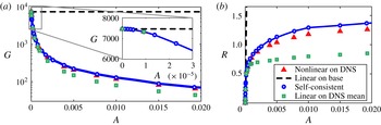
The self-consistent model predicts accurately the response and gain of the exact DNS capturing the strong nonlinear effects of the saturation as depicted in figure 5. The coupling between the mean flow and response equation inherent to the semi-linear model overcomes the limitations of the weakly nonlinear theory. The linear response (4.2) around the saturated DNS mean flow
 $\boldsymbol{U}_{DNS}$
at each forcing amplitude
 $A$
as already presented in § 4 in figure 4 is also compared to the self-consistent model in figure 5 for larger forcing amplitudes. It overpredicts the saturation (figure 5
b), providing a poorer estimation of the gain and response amplitude when compared to the present semi-linear model. This discrepancy could be in large part because the linear response is calculated a posteriori and decoupled from the mean flow equation, suggesting that the coupling between the mean flow and perturbation equation present in the self-consistent model and also in the exact DNS is relevant. Figure 5 confirms the picture of the proposed self-consistent model in which the Reynolds stress plays the main role in the saturation process while higher harmonic interactions are negligible.
(a) Gain and (b) response saturation as functions of forcing amplitude
 $A$
for DNS (triangles) compared to self-consistent results (solid line with circles) and linear response
 $u_{1DNS}$
around the saturated mean flow from DNS (squares). Forcing with optimal structure at frequency
 $f=0.075$
and
 $Re=500$
.

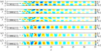
The spatial distribution of the saturated response calculated by the self-consistent model accurately predicts the full nonlinear DNS as presented in figure 6 for a forcing
 $A=0.01$
. The wavelength and the position of the largest amplification of the self-consistent response match the exact DNS solution for both
 $u_{x}^{\prime }$
and
 $u_{y}^{\prime }$
fluctuations. The linear response around the DNS mean flow also resembles the full DNS structure, despite its less accurate approximation of the saturated gain (figure 5
b). It should be noted that these discrepancies are minimal when compared to the structure of the linear response around the base flow as illustrated in figure 3.
Comparison of the response structure in the
 $x$
and
 $y$
directions for the self-consistent model
 $u_{1}$
(a,d), snapshot of the DNS
 $u^{\prime }$
(b,e), and linear response around the DNS mean flow
 $u_{1DNS}$
(c,f). High saturation level with a forcing amplitude
 $A=0.01$
, frequency
 $St=0.075$
and
 $Re=500$
.

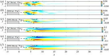
As illustrated in figure 3, the Reynolds stress varies strongly with the forcing amplitude; however, thanks to the coupling present in the semi-linear model, the structure of the Reynolds stress divergence of the DNS and self-consistent model compare very closely as depicted in figure 7. In this case, the Reynolds stress divergence calculated from the linear prediction around the mean flow differs substantially from the exact DNS solution. The Reynolds stress forcing is crucial to obtain the accurate mean flow with the correct recirculation region and thus, through a proper coupling, the corresponding response.
Comparison of the Reynolds stress divergence structure in the
 $x$
and
 $y$
directions for the self-consistent model
 $2\,\text{Re}((\bar{\boldsymbol{u}}_{1}\boldsymbol{\cdot }\boldsymbol{{\rm\nabla}})\boldsymbol{u}_{1})$
(a,d), exact average from the DNS
 $\langle (\boldsymbol{u}^{\prime }\boldsymbol{\cdot }\boldsymbol{{\rm\nabla}})\boldsymbol{u}^{\prime }\rangle$
(b,e), and construction from the linear response around the DNS mean flow
 $2\,\text{Re}((\bar{\boldsymbol{u}}_{1DNS}\boldsymbol{\cdot }\boldsymbol{{\rm\nabla}})\boldsymbol{u}_{1DNS})$
(c,f). High saturation level with a forcing amplitude
 $A=0.01$
, frequency
 $St=0.075$
and
 $Re=500$
.

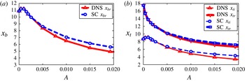
A more quantitative comparison between the self-consistent model and DNS mean flow is summarized in figure 8, where the positions of the recirculation regions are depicted as a function of the forcing amplitude. The self-consistent model approximates precisely the exact recirculation bubbles of the nonlinear DNS. This results from the accurate calculation of the Reynolds stress by the self-consistent model which provides the correct mean flow. At high forcing the saturation is very strong and higher-order nonlinear effects, which are neglected in the semi-linear model, start playing an more important role, explaining the slight divergence between the self-consistent model results and the DNS. Nevertheless, the self-consistent model captures even the non-monotonic trend of the recirculation bubble position present in the exact DNS solutions, which would be missed by a linear prediction around the base flow.
Positions of the bottom (a) and top (b) recirculation bubbles, as a function of the forcing amplitude
 $A$
for the DNS and self-consistent model for the optimal forcing frequency
 $St=0.075$
and
 $Re=500$
.

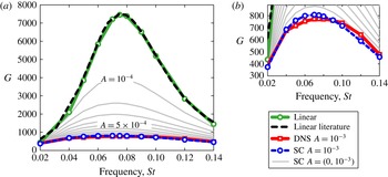
The frequency dependence of the saturation process of the gain starting from the linear prediction to a forcing amplitude
 $A=0.001$
is presented in figure 9. The comparison of the self-consistent saturated gain and the DNS for
 $A=0.001$
in figure 9 shows a very accurate prediction at all frequencies, with only a slight shift in the optimal frequency. More generally, figure 9 demonstrates that the most responsive frequency does not change much when nonlinear effects are included, as pointed out by the preliminary results of Marquet, Sipp & Lesshafft (Reference Marquet, Sipp and Lesshafft2010) using random noise forced DNS.
Gain saturation as a function of frequency for several forcing amplitudes
 $A$
, ranging from 0 to
 $A=\cdot 10^{-3}$
in equal intervals. The DNS results are compared to the self-consistent and linear response around the base flow, from the literature. The forcing applied has its optimal structure at each frequency and
 $Re=500$
.

6 Discussion and conclusions
A study of the saturation dynamics of the response to harmonic forcing is performed for the stable laminar flow over a backward-facing step. An asymptotic expansion around the stable base flow suggests that, at least for very small forcing amplitudes, the saturation dynamics is driven by the mean flow modification enforced by the Reynolds stress and not by the higher harmonic interaction. This is confirmed at larger forcing amplitudes, as the linear response to harmonic forcing around the mean flow extracted from DNS shows a good prediction of the response amplitude and structure.
Motivated by the results of the linear response around the DNS mean flow, a self-consistent model is introduced where the mean flow equation is coupled to the linear response through the Reynolds stress. The coupled equations are solved by an iterative method. The linear response, around its corresponding coupled mean flow, approximates accurately the fully nonlinear response of the exact DNS simulations in terms of gain and structure. Contrary to the weakly nonlinear theory, the self-consistent model solution is not restricted to a small amplitude of the harmonic forcing. Furthermore, the self-consistent model calculates the precise Reynolds stress forcing, which in turn allows one to obtain the correct mean flow as compared to the exact DNS, predicting an accurate recirculation bubble shortening related to the saturation mechanism.
The results of the self-consistent model highlight the Reynolds stress as the driving force for the response saturation in a forced backward-facing step flow, in the same fashion as the case of the cylinder wake flow reported in Mantič-Lugo et al. (Reference Mantič-Lugo, Arratia and Gallaire2014, Reference Mantič-Lugo, Arratia and Gallaire2015), where a conceptually similar model is applied to the unstable cylinder flow with the saturation mechanism of the instability dominated by the most unstable eigenmode as suggested by Stuart (Reference Stuart1958). These oscillators and amplifiers share conceptually a similar saturation mechanism: the growing fluctuation, which can be accurately approximated by the most unstable eigenmode or the linear response respectively, saturates through the modification of the mean flow by the forcing of the Reynolds stress.
A fundamental aspect of the model is that the full nonlinear response of the DNS is approximated by a linear fluctuation equation in the same spirit as the models presented in Farrell & Ioannou (Reference Farrell and Ioannou2012), Thomas et al. (Reference Thomas, Lieu, Jovanović, Farrell, Ioannou and Gayme2014) and Beaume et al. (Reference Beaume, Chini, Julien and Knobloch2015) for asymptotically stable turbulent flows that present coherent structures and for the laminar unstable cylinder flow in Mantič-Lugo et al. (Reference Mantič-Lugo, Arratia and Gallaire2014, Reference Mantič-Lugo, Arratia and Gallaire2015). Furthermore, the full fluctuation is approximated by only the first harmonic because of the linearity, thus neglecting the higher frequency generation. Nevertheless, the self-consistent model is still able to approximate well the nonlinear gain, response and mean flow at different forcing frequencies and amplitudes. While reminiscent of the nonlinear transfer function (the so-called describing function) used to assess the stability of flames in combustion in Noiray et al. (Reference Noiray, Durox, Schuller and Candel2008), it should be highlighted that the self-consistent solution is calculated a priori, without resorting to any DNS or experimental results. The model is not conceived as a substitute for the exact nonlinear DNS. In contrast, its relevance lies in extracting and isolating the essential ingredients to provide an accurate description of the physics, and thus clarifying the different physical mechanisms involved in the saturation process.
It remains to be seen whether the present semi-linear model works for other globally stable laminar flows excited by harmonic forcing, i.e. jets, etc., providing the response is quasi-monochromatic. However, it is not expected to work directly for turbulent or chaotic flows unless a separation of scales is applied and turbulent and coherent Reynolds stress terms are calculated independently.
Appendix A. Asymptotic expansion around the base flow
Assuming that the harmonically forced flow reaches a stable limit cycle, an asymptotic expansion is carried around the base flow
 $\boldsymbol{U}_{B}=\boldsymbol{U}_{0}$
in the same fashion as the one used to obtain the amplitude equation for the cylinder flow described in Sipp & Lebedev (Reference Sipp and Lebedev2007). In the amplitude equation the small parameter
 ${\it\epsilon}$
corresponds to the departure from threshold by the Reynolds number modification. In contrast, in the present case the Reynolds number is fixed and the selected small parameter
 ${\it\epsilon}=A$
is the amplitude of the normalized forcing
 $\boldsymbol{f}_{1}$
(§ 2.2).
For the sake of clarity, we separate the steady terms
 $\boldsymbol{U}=\sum _{n=0}^{\infty }{\it\epsilon}^{n}\boldsymbol{u}_{0,n}$
and unsteady terms
 $\boldsymbol{u}^{\prime }=\sum _{n=0}^{\infty }\sum _{p=1}^{\infty }{\it\epsilon}^{n}\boldsymbol{u}_{p,n}\text{e}^{\text{i}p{\it\omega}t}$
of the asymptotic expansion, relating them to mean flow and fluctuation modifications. We use the following notation for
 $\boldsymbol{u}_{p,n}$
: the first subindex
 $p$
corresponds to the frequency and the second subindex
 $n$
corresponds to the order.
A.1 Zeroth order
The zeroth order corresponds to the base flow
 $\boldsymbol{u}_{0,0}=\boldsymbol{U}_{B}$
solution of the steady nonlinear NSE
 $$\begin{eqnarray}\mathscr{N}(\boldsymbol{u}_{0,0})=0.\end{eqnarray}$$
A.2 First order
The first-order solution corresponds to the classical linear response
 ${\it\epsilon}\boldsymbol{u}_{1,1}=\boldsymbol{u}_{1B}$
(§ 2.2) or first harmonic with the same frequency as the forcing
 $\boldsymbol{f}_{1}={\it\epsilon}\boldsymbol{f}_{1,1}$
with amplitude
 ${\it\epsilon}=A$
,
 $$\begin{eqnarray}{\it\epsilon}[\text{i}{\it\omega}+\mathscr{L}_{\boldsymbol{U}_{B}}]\boldsymbol{u}_{1,1}={\it\epsilon}\boldsymbol{f}_{1,1}.\end{eqnarray}$$
Note that there is no mean flow contribution at first order,
 $\boldsymbol{u}_{0,1}=0$
.
A.3 Second order
The second order has two terms, one steady and one unsteady. Both terms are forced by the interaction of the first-order response with itself, as
 $$\begin{eqnarray}\displaystyle & \displaystyle {\it\epsilon}^{2}\mathscr{L}_{\boldsymbol{U}_{B}}\boldsymbol{u}_{0,2}=-{\it\epsilon}^{2}((\bar{\boldsymbol{u}}_{1,1}\boldsymbol{\cdot }\boldsymbol{{\rm\nabla}})\boldsymbol{u}_{1,1}+(\boldsymbol{u}_{1,1}\boldsymbol{\cdot }\boldsymbol{{\rm\nabla}})\bar{\boldsymbol{u}}_{1,1})=-{\it\epsilon}^{2}\boldsymbol{F}_{\boldsymbol{u}_{1,1}}, & \displaystyle\end{eqnarray}$$
 $$\begin{eqnarray}\displaystyle & \displaystyle {\it\epsilon}^{2}[\text{i}2{\it\omega}+\mathscr{L}_{\boldsymbol{U}_{B}}]\boldsymbol{u}_{2,2}=-{\it\epsilon}^{2}(\boldsymbol{u}_{1,1}\boldsymbol{\cdot }\boldsymbol{{\rm\nabla}})\boldsymbol{u}_{1,1}, & \displaystyle\end{eqnarray}$$
 $\overline{(.)}$
means complex conjugate. The steady term (A 3a
) corresponds to the modification of the base flow to the mean flow due to the steady Reynolds stress forcing
 $\boldsymbol{F}_{\boldsymbol{u}_{1,1}}$
, whilst the unsteady term (A 3b
) corresponds to the second harmonic
 $\boldsymbol{u}_{2,2}^{\prime }={\it\epsilon}^{2}\boldsymbol{u}_{2,2}\text{e}^{\text{i}2{\it\omega}t}+\text{c.c.}$
oscillating at double frequency
 $2{\it\omega}$
. It appears as a solution of the linear system slaved by the forcing of the first harmonic interacting with itself.
A.4 Third order
The third order presents two unsteady equations:
 $$\begin{eqnarray}\displaystyle {\it\epsilon}^{3}[\text{i}{\it\omega}+\mathscr{L}_{\boldsymbol{U}_{B}}]\boldsymbol{u}_{1,3} & = & \displaystyle -{\it\epsilon}^{3}((\boldsymbol{u}_{0,2}\boldsymbol{\cdot }\boldsymbol{{\rm\nabla}})\boldsymbol{u}_{1,1}+(\boldsymbol{u}_{1,1}\boldsymbol{\cdot }\boldsymbol{{\rm\nabla}})\boldsymbol{u}_{0,2})\nonumber\\ \displaystyle & & \displaystyle -\,{\it\epsilon}^{3}((\boldsymbol{u}_{2,2}\boldsymbol{\cdot }\boldsymbol{{\rm\nabla}})\bar{\boldsymbol{u}}_{1,1}+(\bar{\boldsymbol{u}}_{1,1}\boldsymbol{\cdot }\boldsymbol{{\rm\nabla}})\boldsymbol{u}_{2,2}),\end{eqnarray}$$
 $$\begin{eqnarray}\displaystyle {\it\epsilon}^{3}[\text{i}3{\it\omega}+\mathscr{L}_{\boldsymbol{U}_{B}}]\boldsymbol{u}_{3,3} & = & \displaystyle -{\it\epsilon}^{3}((\boldsymbol{u}_{2,2}\boldsymbol{\cdot }\boldsymbol{{\rm\nabla}})\boldsymbol{u}_{1,1}+(\boldsymbol{u}_{1,1}\boldsymbol{\cdot }\boldsymbol{{\rm\nabla}})\boldsymbol{u}_{2,2}).\end{eqnarray}$$
 $-{\it\epsilon}^{3}((\boldsymbol{u}_{0,2}\boldsymbol{\cdot }\boldsymbol{{\rm\nabla}})\boldsymbol{u}_{1,1}+(\boldsymbol{u}_{1,1}\boldsymbol{\cdot }\boldsymbol{{\rm\nabla}})\boldsymbol{u}_{0,2})$
, relates to the mean flow modification due to the Reynolds stress; in other words, it accounts for the nonlinear interaction on the right-hand side of the mean flow steady equation (4.1a
). The second forcing term,
 $-{\it\epsilon}^{3}((\boldsymbol{u}_{2,2}\boldsymbol{\cdot }\boldsymbol{{\rm\nabla}})\bar{\boldsymbol{u}}_{1,1}+(\bar{\boldsymbol{u}}_{1,1}\boldsymbol{\cdot }\boldsymbol{{\rm\nabla}})\boldsymbol{u}_{2,2})$
, corresponds to the interaction of the first harmonic
 $\boldsymbol{u}_{1,1}\text{e}^{\text{i}{\it\omega}t}$
with the second
 $\boldsymbol{u}_{2,2}\text{e}^{\text{i}2{\it\omega}t}$
.
Equation (A 4b
) at third order corresponds to the third harmonic oscillating at three times the forcing frequency
 $3{\it\omega}$
. It is slaved by the interactions of the first
 ${\it\omega}$
and second
 $2{\it\omega}$
harmonic.
A.5 Synthesis
Stopping at the third order, our asymptotic expansion can be summarized as
 $$\begin{eqnarray}\displaystyle & \displaystyle \boldsymbol{U}(\boldsymbol{x})\simeq \boldsymbol{u}_{0,0}(\boldsymbol{x})+{\it\epsilon}^{2}\boldsymbol{u}_{0,2}(\boldsymbol{x}), & \displaystyle\end{eqnarray}$$
 $$\begin{eqnarray}\displaystyle & \displaystyle \boldsymbol{u}^{\prime }(\boldsymbol{x},t)\simeq {\it\epsilon}\boldsymbol{u}_{1,1}(\boldsymbol{x})\text{e}^{\text{i}{\it\omega}t}+{\it\epsilon}^{2}\boldsymbol{u}_{2,2}(\boldsymbol{x})\text{e}^{\text{i}2{\it\omega}t}+{\it\epsilon}^{3}(\boldsymbol{u}_{1,3}(\boldsymbol{x})\text{e}^{\text{i}{\it\omega}t}+\boldsymbol{u}_{3,3}(\boldsymbol{x})\text{e}^{\text{i}3{\it\omega}t})+\text{c.c.}\quad & \displaystyle\end{eqnarray}$$
 $$\begin{eqnarray}G_{3ord}^{2}=\frac{\Vert \boldsymbol{u}^{\prime }\Vert ^{2}}{\Vert \,\boldsymbol{f}\Vert ^{2}}=G_{1}^{2}\left(1+\frac{{\it\epsilon}^{2}}{G_{1}^{2}}(K_{2,2}+K_{1,3})\right),\end{eqnarray}$$
where
 $$\begin{eqnarray}K_{2,2}=\frac{\displaystyle \int _{{\it\Omega}}\boldsymbol{u}_{2,2}^{2}\,\text{d}{\it\Omega}}{\Vert \,\boldsymbol{f}_{1,1}\Vert ^{2}}=1.2\times 10^{14}\quad \text{and}\quad K_{1,3}=\frac{\displaystyle \int _{{\it\Omega}}2\boldsymbol{u}_{1,1}\boldsymbol{\cdot }\boldsymbol{u}_{1,3}\,\text{d}{\it\Omega}}{\Vert \,\boldsymbol{f}_{1,1}\Vert ^{2}}=-2.5\times 10^{16}.\end{eqnarray}$$
Here
 $K_{2,2}$
is the gain correction due to the energy of the second harmonic while
 $K_{1,3}$
relates to energy modification due to the correction of the first harmonic at third order (A 4a
). In figure 10 are compared the linear gain
 $G_{1}$
, the saturation of the fully nonlinear DNS gain
 $G_{DNS}$
and the weakly nonlinear gain correction at third order
 $G_{3ord}$
. As one could expect, the weakly nonlinear theory predicts well the initial saturation trend for small forcing amplitudes
 ${\it\epsilon}$
, and it starts failing for larger forcing amplitudes. Figure 10 illustrates how the influence of the second harmonic is small compared to the first harmonic modification at third order, since the elimination of its correction factor
 $K_{2,2}$
does not produce any change to the saturation curve,
 $|K_{2,2}|\ll |K_{1,3}|$
. We thus neglect the influence of the second and third harmonic of (A 5b
) and restrict our attention to the response at the same frequency as the forcing (A 4a
). We observe that
 $K_{1,3}<0$
indeed accounts for the saturation.
Gain of the response for the optimal forcing at frequency
 $St=0.075$
and
 $Re=500$
. Linear prediction (dash-dotted line), third-order weakly nonlinear correction (squares), third-order weakly nonlinear correction of the first harmonic only at the forcing frequency (circles), third-order weakly nonlinear correction only by second harmonic interaction (
 $\times$
), third-order weakly nonlinear correction only by mean flow modification (
 $+$
) and DNS results (triangles).

As expressed above, the third-order adjustment of the response results from two different physical phenomena: the interaction of the second harmonic with the first one corresponding to
 $(\boldsymbol{u}_{2,2}\boldsymbol{\cdot }\boldsymbol{{\rm\nabla}})\bar{\boldsymbol{u}}_{1,1}+(\bar{\boldsymbol{u}}_{1,1}\boldsymbol{\cdot }\boldsymbol{{\rm\nabla}})\boldsymbol{u}_{2,2}$
, and the interaction of the first harmonic with the steady mean flow modification corresponding to
 $(\boldsymbol{u}_{0,2}\boldsymbol{\cdot }\boldsymbol{{\rm\nabla}})\boldsymbol{u}_{1,1}+(\boldsymbol{u}_{1,1}\boldsymbol{\cdot }\boldsymbol{{\rm\nabla}})\boldsymbol{u}_{0,2}$
. We can separate them and account independently for their role in the saturation process due to the linearity of the problem. The third-order term forced only by the interaction of the first harmonic with the second reads
 $$\begin{eqnarray}{\it\epsilon}^{3}[\text{i}{\it\omega}+\mathscr{L}_{\boldsymbol{ U}_{0}}]\boldsymbol{u}_{1,3}^{(2)}=-{\it\epsilon}^{3}((\boldsymbol{u}_{2,2}\boldsymbol{\cdot }\boldsymbol{{\rm\nabla}})\bar{\boldsymbol{u}}_{1,1}+(\bar{\boldsymbol{u}}_{1,1}\boldsymbol{\cdot }\boldsymbol{{\rm\nabla}})\boldsymbol{u}_{2,2}),\end{eqnarray}$$
and the new gain modification factor
 $K_{1,3}^{(2)}$
corresponds to
 $$\begin{eqnarray}K_{1,3}^{(2)}=\frac{\displaystyle \int _{{\it\Omega}}2\boldsymbol{u}_{1,1}\boldsymbol{\cdot }\boldsymbol{u}_{1,3}^{(2)}\,\text{d}{\it\Omega}}{\Vert \,\boldsymbol{f}_{1,1}\Vert ^{2}}=-8.7\times 10^{13}\end{eqnarray}$$
accounting only for the second harmonic interacting with the first. Figure 10 shows how the new gain adjusted exclusively by the second harmonic interaction with the first has a negligible nonlinear effect for the saturation, following mainly the linear prediction.
The third-order term forced only by the mean flow modification reads
 $$\begin{eqnarray}{\it\epsilon}^{3}[\text{i}{\it\omega}+\mathscr{L}_{\boldsymbol{ U}_{0}}]\boldsymbol{u}_{1,3}^{(0)}=-{\it\epsilon}^{3}((\boldsymbol{u}_{0,2}\boldsymbol{\cdot }\boldsymbol{{\rm\nabla}})\boldsymbol{u}_{1,1}+(\boldsymbol{u}_{1,1}\boldsymbol{\cdot }\boldsymbol{{\rm\nabla}})\boldsymbol{u}_{0,2}),\end{eqnarray}$$
and thus a new gain modification factor
 $K_{1,3}^{(0)}$
,
 $$\begin{eqnarray}K_{1,3}^{(0)}=\frac{\displaystyle \int _{{\it\Omega}}2\boldsymbol{u}_{1,1}\boldsymbol{\cdot }\boldsymbol{u}_{1,3}^{(0)}\,\text{d}{\it\Omega}}{\Vert \,\boldsymbol{f}_{1,1}\Vert ^{2}}=-2.5\times 10^{16},\end{eqnarray}$$
can be retrieved accounting solely for the mean flow modification effect. Figure 10 shows how the new gain adjusted exclusively by the mean flow modification follows precisely the curve of the full third-order gain, since
 $K_{1,3}^{(2)}\ll K_{1,3}^{(0)}\sim K_{1,3}$
. It therefore appears that the nonlinear saturation process is captured mainly by the Reynolds stress modification and not by the second harmonic interaction, highlighting the importance of the mean flow in the saturation process in a similar way as for the cylinder flow (Barkley Reference Barkley2006; Mantič-Lugo et al.
Reference Mantič-Lugo, Arratia and Gallaire2014, Reference Mantič-Lugo, Arratia and Gallaire2015).